Coding of nonlinear states for the Gross-Pitaevskii equation with periodic potential

Abstract

We study nonlinear states for NLS-type equation with additional periodic potential $U(x)$ (called the Gross-Pitaevskii equation, GPE in theory of Bose-Einstein Condensate, BEC). We prove that if the nonlinearity is defocusing (repulsive, in BEC context) then under certain conditions there exists a homeomorphism between the set of nonlinear states for GPE (i.e. real bounded solutions of some nonlinear ODE) and the set of bi-infinite sequences of numbers from 1 to $N$ for some integer $N$. These sequences can be viewed as codes of the nonlinear states. Sufficient conditions for the homeomorphism to exist are given in the form of three hypotheses. For a given $U(x)$, the verification of the hypotheses should be done numerically. We report on numerical results for the case of GPE with cosine potential and describe regions in the plane of parameters where this coding is possible.

1 Introduction

The nonlinear Schrödinger equation with additional potential $U({\bf x})$,

$$i\Psi_{t}=-\Delta\Psi+U({\bf x})\Psi+\sigma|\Psi|^{2}\Psi,$$ (1)

$$\Delta\equiv\frac{\partial^{2}\,}{\partial x^{2}}+\frac{\partial^{2}\,}{\partial y^{2}}+\frac{\partial^{2}\,}{\partial z^{2}},\quad\sigma=\pm 1$$

arises in many physical applications including models of optics [1], plasma physics [2] and theory of ultracold gases [3]. In the last context, Eq.(1) (called the Gross-Pitaevskii equation, GPE) appears as one of the basic equations to describe the phenomenon of Bose-Einstein condensation (BEC) in so-called mean-field approximation. In this case $\Psi(t,{\bf x})$ means the macroscopic wave function of the condensate, $\sigma=1$ corresponds to the case of to repulsive interparticle interactions and $\sigma=-1$ - to the case of attractive interactions. The function $U({\bf x})$ describes the potential of the trap to confine the condensate. In particular, magnetic trap has been modelled by the parabolic potential $U({\bf x})=|{\bf x}|^{2}$ and optical trap has been described by the potential which is periodic with respect to one or several variables [4, 5, 6].

An important class of solutions for Eq.(1) are stationary nonlinear states defined by the anzats

$$\Psi(t,{\bf x})=e^{-i\omega t}\psi({\bf x}).$$ (2)

The parameter $\omega$ in terms of BEC corresponds to the chemical potential. The function $\psi({\bf x})$ solves the equation

$$\Delta\psi+(\omega-U({\bf x}))\psi-\sigma|\psi|^{2}\psi=0.$$ (3)

It is known that Eq.(3) describes a great variety of nonlinear objects. In particular, it has been found that real 1D-version of Eq.(3)

$$\psi_{xx}+(\omega-U(x))\psi-\sigma\psi^{3}=0$$ (4)

with the model cosine potential

$$U(x)=A\cos 2x$$ (5)

describes bright and dark gap solitons [7, 8, 9, 10], nonlinear periodic structures (nonlinear Bloch waves) [7, 11], domain walls [12], gap waves [13] and so on. Some interesting relations between various nonlinear objects described by Eq.(4) have been observed. In particular, in papers [14, 15] the composition relation between gap solitons and nonlinear Bloch waves was established: it has been observed that a nonlinear Bloch wave can be approximated by an infinite chain of narrow gap solitons (called fundamental gap solitons, FGS), each localized in one well of the periodic potential. In [16] this principle has been applied to the case of more general nonlinearity. It is worth noting that the results of [13] also can be interpreted in a similar sense, since the gap waves discovered in [13] can be regarded as compositions of finite number of FGS.

In the present paper, we address the problem of description of nonlinear states covered by Eq.(4) in the case of repulsive interactions, $\sigma=1$, i.e for the equation

$$\psi_{xx}+(\omega-U(x))\psi-\psi^{3}=0.$$ (6)

We argue that if the periodic potential $U(x)$ satisfies some conditions, then all the solutions of Eq.(6) defined at the whole $\mathbb{R}$ can be put in one-to-one correspondence with bi-infinite sequences of integers $n=1,\ldots,N$ (called codes). The correspondence is a homeomorphism for properly introduced topological spaces. Each of the integers $n$ is “responsible” for the behavior of the solution $\psi(x)$ on one period of the potential $U(x)$. From this viewpoint, the solutions $\psi(x)$ may be regarded as compositions of FGS localized in the wells of the periodic potential and taken with a proper sign. So, the coding technique gives a unified approach to describe both gap solitons and nonlinear Bloch waves and generalizes (and justifies) the composition relation of [14, 15]. In order to conclude that for a given $U(x)$ the coding is possible, one has to verify numerically three Hypotheses formulated in Section 4. As an example, we applied this method to the case of model periodic potential (5) and present the regions in the parameter plane $(\omega,A)$ where all nonlinear states can be encoded with bi-infinite sequences of integers.

Our approach is based on the following observation: the “most part” of the solutions for Eq.(6) are singular, i.e. they collapse (tend to infinity) at some finite point of real axis. The set of initial data at $x=0$ for non-collapsing solutions can be found numerically by properly organized scanning procedure. Then we study transformations of this set under the action of Poincare map using methods of symbolic dynamics. A similar idea was used to justify a strategy of “demonstrative computations” of nonlinear modes for 1D GPE with repulsive interactions and multi-well potential [17, 18]. This allowed to find numerically all the localized modes for Eq.(6) with single-well and double-well potentials and to guarantee that no other localized modes exist.

The paper is organized as follows. In Section 2 we introduce some notations and definitions which will be used throughout the rest of the text and make some assertions about them. In Section 3 we formulate a theorem (Theorem 3.1) which gives a base for our method. Section 4 contains an application of Theorem 3.1 to the case of Eq.(6). The main outcome of Section 4 is formulated in the form of three hypotheses. These hypotheses provide sufficient conditions for the homeomorphism mentioned above to exist and should be verified numerically. In Section 5 we apply this approach to the case of the cosine potential (5). Section 6 includes summary and discussion.

For the sake of clarity all the proofs are removed from the main text to Appendices.

2 Bounded and singular solutions

2.1 Some definitions

In what follows we refer to a solution $\psi(x)$ of Eq.(6) as a singular solution if for some $x=x_{0}$

$$\lim_{x\to x_{0}}\psi(x)=+\infty\quad\mbox{or}\quad\lim_{x\to x_{0}}\psi(x)=-\infty.$$

In this case we say that the solution $\psi(x)$ collapses at $x_{0}$. Also let us introduce the following definitions:

Collapsing and non-collapsing points: A point $(\psi_{0},\psi_{0}^{\prime})$ of the plane $\mathbb{R}^{2}=(\psi,\psi^{\prime})$ is

• $L$-collapsing forward point, $L>0$, if the solution of Cauchy problem for Eq.(6) with initial data $\psi(0)=\psi_{0}$, $\psi_{x}(0)=\psi_{0}^{\prime}$ collapses at value $x=x_{0}$ and $0<x_{0}<L$;

• $L$-non-collapsing forward point, $L>0$, if the solution of Cauchy problem for Eq.(6) with initial data $\psi(0)=\psi_{0}$, $\psi_{x}(0)=\psi_{0}^{\prime}$ does not collapse at any value $x=x_{0}$, $0<x_{0}\leq L$.

• $L$-collapsing backward point if the corresponding solution of Cauchy problem for Eq.(6) collapses at some value $x=-x_{0}$ and $0<x_{0}<L$;

• $L$-non-collapsing backward point if the corresponding solution of Cauchy problem for Eq.(6) does not collapse at any value $x=-x_{0}$, $0<x_{0}\leq L$;

• $\infty$-non-collapsing forward/backward point if it is not $L$-collapsing forward/backward point for any $L>0$;

• $\infty$-non-collapsing point if it is a $\infty$-non-collapsing forward and backward point simultaneously;

• a collapsing point if it is either $L$-collapsing forward or backward for some $L$.

Functions $h^{\pm}(\tilde{\psi},\tilde{\psi}^{\prime})$. The functions $h^{+}(\tilde{\psi},\tilde{\psi}^{\prime})$ and $h^{-}(\tilde{\psi},\tilde{\psi}^{\prime})$ are defined in ${\mathbb{R}}^{2}$ as follows: $h^{+}(\tilde{\psi},\tilde{\psi}^{\prime})=x_{0}$ if the solution of Cauchy problem for Eq.(6) with initial data $\psi(0)=\tilde{\psi}$, $\psi_{x}(0)=\tilde{\psi}^{\prime}$ collapses at value $x=x_{0}$, $x_{0}>0$. By convention, we assume that $h^{+}(\tilde{\psi},\tilde{\psi}^{\prime})=\infty$ if $(\tilde{\psi},\tilde{\psi}^{\prime})$ is $\infty$-non-collapsing forward point. Similarly, $h^{-}(\tilde{\psi},\tilde{\psi}^{\prime})=-x_{0}$ if the solution of Cauchy problem for Eq.(6) with initial data $\psi(0)=\tilde{\psi}$, $\psi_{x}(0)=\tilde{\psi}^{\prime}$ collapses at value $x=x_{0}$, $x_{0}<0$.

The sets ${\cal U}_{L}^{\pm}$ and ${\cal U}_{L}$. We denote the set of all $L$-non-collapsing forward points by ${\cal U}_{L}^{+}$ and the set of all $L$-non-collapsing backward points by ${\cal U}_{L}^{-}$. In terms of the functions $h^{\pm}(\psi,\psi^{\prime})$ these sets are

$${\cal U}^{+}_{L}=\{(\psi,\psi^{\prime})\in\mathbb{R}^{2}|~{}h^{+}(\psi,\psi^{\prime})>L\},\quad{\cal U}^{-}_{L}=\{(\psi,\psi^{\prime})\in\mathbb{R}^{2}|~{}h^{-}(\psi,\psi^{\prime})>L\}.$$

The intersection of ${\cal U}_{L}^{+}$ and ${\cal U}_{L}^{-}$ will be denoted by ${\cal U}_{L}$. Evidently, if $L_{1}<L_{2}$ then ${\cal U}^{+}_{L_{2}}\subset{\cal U}^{+}_{L_{1}}$, ${\cal U}^{-}_{L_{2}}\subset{\cal U}^{-}_{L_{1}}$ and ${\cal U}_{L_{2}}\subset{\cal U}_{L_{1}}$.

The values $\overline{\Omega}$ and $\underline{\Omega}$. We define

$$\overline{\Omega}\equiv\sup_{x\in{\mathbb{R}}}(\omega-U(x)),\quad\underline{\Omega}\equiv\inf_{x\in{\mathbb{R}}}(\omega-U(x)).$$

2.2 Some statements about collapsing points

In what follows we will use some statements from the paper [17], in particular so-called Comparison Lemma (reproduced in A for convenience). It is known [17] that for $\overline{\Omega}<0$ Eq.(6) has no bounded on $\mathbb{R}$ solutions, therefore we restrict our analysis by the case $\overline{\Omega}\geq 0$. Also it is known ([17], Lemma 2) that all $\infty$-non-collapsing points for Eq.(6) are situated in the strip $-\sqrt{\overline{\Omega}}\leq\psi\leq\sqrt{\overline{\Omega}}$. Theorem 2.1 below gives more detailed information about collapsing points for Eq.(6).

Theorem 2.1. Let the potential $U(x)$ be continuous and bounded on $\mathbb{R}$. Then for each $L$ there exist $\tilde{\psi}_{L}$ and $\tilde{\psi}^{\prime}_{L}$ such that the set ${\cal U}_{L}$ is situated in the rectangle $-\tilde{\psi}_{L}<\psi<\tilde{\psi}_{L}$, $-\tilde{\psi}^{\prime}_{L}<\psi^{\prime}<\tilde{\psi}^{\prime}_{L}$.

The proof of Theorem 2.1 is quite technical. We postponed it in A.

Another important statement is as follows:

Theorem 2.2. Let the potential $U(x)$ be continuous and bounded on $\mathbb{R}$ and $h^{+}(\psi_{0},\psi^{\prime}_{0})=L<\infty$. Then $h^{+}(\psi,\psi^{\prime})$ is a continuous function in some vicinity of the point $(\psi_{0},\psi^{\prime}_{0})$.

The proof of Theorem 2.2 can be found in B. It is worth commenting Theorem 2.2 as follows:

(i) Analogous statement is valid for the function $h^{-}(\psi,\psi^{\prime})$.

(ii) It follows from Theorem 2.2 that if the potential $U(x)$ is continuous and bounded on $\mathbb{R}$ then ${\cal U}_{L}^{\pm}$ and ${\cal U}_{L}$ are open sets. The boundary of the set ${\cal U}_{L}^{+}$ consists of continuous curves and corresponds to the level lines $h^{+}(\psi,\psi^{\prime})=L$ of the function $h^{+}(\psi,\psi^{\prime})$. This boundary consists of the points $(\tilde{\psi},\tilde{\psi}^{\prime})$ such that the solution of Eq.(6) with initial data $\psi(0)=\tilde{\psi}$, $\psi_{x}(0)=\tilde{\psi}^{\prime}$ satisfies one of the conditions

$$\lim_{x\to L}\psi(x)=+\infty\quad\mbox{or}\quad\lim_{x\to L}\psi(x)=-\infty.$$

Correspondingly, the boundary of the set ${\cal U}_{L}^{-}$ is also continuous and consists of the points $(\tilde{\psi},\tilde{\psi}^{\prime})$ such that the solution of Eq.(6) with initial data $\psi(0)=\tilde{\psi}$, $\psi_{x}(0)=\tilde{\psi}^{\prime}$ satisfies similar conditions

$$\lim_{x\to-L}\psi(x)=+\infty\quad\mbox{or}\quad\lim_{x\to-L}\psi(x)=-\infty.$$

(iii) Theorem 2.2 does not impose any restriction to the behavior of $h^{+}(\psi,\psi^{\prime})$ in a vicinity of a point $(\psi_{0},\psi^{\prime}_{0})$ where $h^{+}(\psi_{0},\psi^{\prime}_{0})=\infty$. In practice, this behavior may be very complex, see Sect.2.3.2.

The set of solutions for Eq.(6) that collapse at a given point $x=x_{0}$ can be described more precisely in terms of asymptotic expansions.

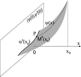
Figure 1: The point $P$, the manifold $M^{+}(x_{0})$, the curve $\alpha^{+}(x_{0})$.

Theorem 2.3. Let $x=x_{0}$ be an arbitrary fixed real. Assume that $\tilde{U}(x)=\omega-U(x)$ in a vicinity of $x=x_{0}$ can be represented as follows

$$\tilde{U}(x)=U_{0}+U_{1}\delta+U_{2}\delta^{2}+U_{3}\delta^{3}+o\left(\delta^{3}\right)$$

where $\delta\equiv x-x_{0}$. Then the solutions of Eq.(6) which satisfy the condition

$$\lim_{x\to x_{0}}\psi(x)=+\infty$$ (7)

obey the asymptotic expansion

$$\psi(\delta) = \frac{\sqrt{2}}{\delta}+A_{1}\delta+A_{2}\delta^{2}+A_{3}\delta^{3}\ln|\delta|+{\bf C}\delta^{3}+A_{4}\delta^{4}+o\left(\delta^{4}\right).$$ (8)

Here ${\bf C}\in\mathbb{R}$ is a free parameter and

$$A_{1}=\frac{\sqrt{2}U_{0}}{6};\quad A_{2}=\frac{\sqrt{2}U_{1}}{4};\quad A_{3}=-\frac{\sqrt{2}U_{2}}{5},\quad A_{4}=\frac{\sqrt{2}}{6}\left(\frac{U_{0}U_{1}}{12}-U_{3}\right).$$

Proof: The result follows from straightforward substitution of series (8) into Eq.(6). $\blacksquare$

Theorem 2.3 should be commented as follows.

(i) The free parameter ${\bf C}$ is “internal” parameter of continuous one-parameter set of solutions which tend to $+\infty$ at the point $x=x_{0}$. This situation can be illustrated by the following heuristic reasoning. Let $P=(\psi_{0},\psi_{0}^{\prime})$ be a collapsing point and the solution $\psi(x)$ of Cauchy problem for Eq.(6) with initial data $\psi(0)=\psi_{0}$, $\psi_{x}(0)=\psi_{0}^{\prime}$ collapses at $x=x_{0}>0$. Then, generically $\psi(x)$ belongs to a continuous one-parameter set of solutions which also satisfy the condition (7) and obey the expansion (8). In 3D space $(x,\psi,\psi^{\prime})$ this set generates 2D manifold $M^{+}(x_{0})$ (see Fig.1). Intersection of $M^{+}(x_{0})$ with the plane $(\psi,\psi^{\prime})$ at $x=0$ includes the point $P$ and is non-empty. Generically, this intersection in some vicinity of $P$ is an 1D curve which we denote $\alpha^{+}(x_{0})$. In the plane $(\psi,\psi^{\prime})$ this curve corresponds to the level line $h^{+}(\psi,\psi^{\prime})=x_{0}$.

(ii) Since Eq.(6) is invariant with respect to the symmetry $\psi\to-\psi$, the solutions of Eq.(6) which satisfy the condition

$$\lim_{x\to x_{0}}\psi(x)=-\infty$$

obey the same, up to sign, asymptotic expansion (8). The corresponding manifold $M^{-}(x_{0})$ and the curve $\alpha^{-}(x_{0})$ are defined in the same way.

2.3 Example: the sets ${\cal U}^{\pm}_{L}$ and ${\cal U}_{L}$ for the cosine potential

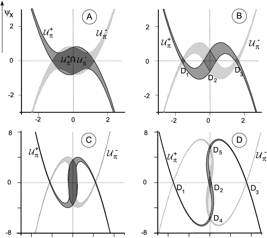
Figure 2: The sets ${\cal U}_{\pi}^{+}$ and ${\cal U}_{\pi}^{-}$ for Eq.(9) and the parameters $\omega$ and $A$ lying in the first (panels A and B) and the second (panels C and D) gaps, see Sect.5 for detail. The parameters are: (A) $\omega=1$, $A=-1$; (B) $\omega=1$, $A=-3$; (C) $\omega=4$, $A=-4$; (D) $\omega=4$, $A=-10$. The sets were obtained numerically by scanning of initial data plane for Eq.(9). The areas ${\cal U}_{\pi}={\cal U}_{\pi}^{+}\cap{\cal U}_{\pi}^{-}$ are shown in dark.

Let us now give now examples of the sets ${\cal U}^{\pm}_{L}$ for Eq.(6) in the case of the cosine potential (5). Eq.(6) takes the form

$$\psi_{xx}+(\omega-A\cos 2x)\psi-\psi^{3}=0.$$ (9)

The sets ${\cal U}^{\pm}_{L}$ possess the following symmetry properties:

• Since the nonlinearity in Eq.(9) is odd, both the sets ${\cal U}_{L}^{\pm}$ are symmetric in the plane $(\psi,\psi^{\prime})$ with respect to the origin;

• Since Eq.(9) is invariant with respect to $x$-inversion the sets ${\cal U}_{L}^{+}$ and ${\cal U}_{L}^{-}$ are related to each other by the symmetry with respect to the axis $\psi$ and due to p.1, with respect to the axis $\psi^{\prime}$ also.

2.3.1 $\pi$-non-collapsing forward/backward points of Eq.(9).

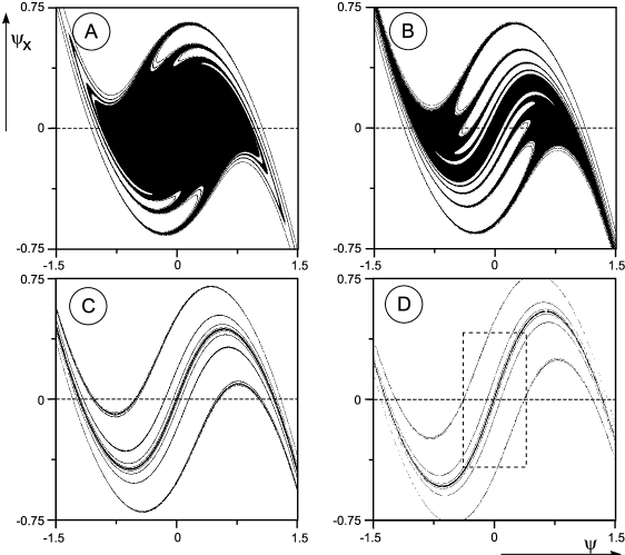
Figure 3: The sets ${\cal U}_{6\pi}^{+}$ for Eq.(9). In all the cases $\omega=1$ and (A) $A=-0.4$; (B) $A=-0.7$; (C) $A=-1.5$; (D) $A=-2.0$. The rectangle in panel D is shown magnified in Fig.12.

The sets ${\cal U}_{\pi}^{\pm}$ were found by thorough numerical scanning in the plane of initial data $(\psi,\psi^{\prime})$ (some details of numerical procedure can be found in Sect.5). The numerical study shows that for any values of parameters $\omega$ and $A$ the sets ${\cal U}_{\pi}^{\pm}$ are infinite curvilinear strips. The typical shapes of the sets ${\cal U}_{\pi}^{\pm}$ for Eq.(9) are shown in Fig.2. The boundary of ${\cal U}_{\pi}^{+}$ is represented by two continuous curves $\alpha^{\pm}$. The curve $\alpha^{+}$ consists of such points $(\psi_{0},\psi^{\prime}_{0})$ that the solution $\psi(x)$ of the Cauchy problem for Eq.(9) with initial data $\psi(0)=\psi_{0}$, $\psi^{\prime}(0)=\psi^{\prime}_{0}$ collapses at $x=\pi$ and $\lim_{x\to\pi}\psi(x)=+\infty$. At the curve $\alpha^{-}$ the solution $\psi(x)$ of the corresponding Cauchy problem obeys the condition $\lim_{x\to\pi}\psi(x)=-\infty$. Similarly, the boundary of ${\cal U}_{\pi}^{-}$ is represented by two continuous curves $\beta^{\pm}$. The curves $\beta^{\pm}$ consist of points $(\psi_{0},\psi^{\prime}_{0})$ such that the solution $\psi(x)$ of the Cauchy problem for Eq.(9) with initial data $\psi(0)=\psi_{0}$, $\psi^{\prime}(0)=\psi^{\prime}_{0}$ collapses at $x=-\pi$ and $\lim_{x\to-\pi}\psi(x)=\pm\infty$.

$\pi$-non-collapsing forward and backward points of Eq.(9) form the set ${\cal U}_{\pi}={\cal U}_{\pi}^{+}\cap{\cal U}_{\pi}^{-}$. It follows from Fig.2 that this set may consist of several disjoined components. More detailed discussion of the sets ${\cal U}_{\pi}^{\pm}$ and ${\cal U}_{\pi}$ is postponed to Sect.5.

2.3.2 $\pi n$-non-collapsing forward/backward points of Eq.(9), $n>1$.

Fig.3 exhibits the sets ${\cal U}_{6\pi}^{+}$ for $\omega=1$ and various values of $A$. The sets ${\cal U}_{6\pi}^{-}$ are the reflections of the sets ${\cal U}_{6\pi}^{+}$ with respect to the $\psi$ axis. It follows from Fig.3 that the sets ${\cal U}_{6\pi}^{\pm}$ have quite a complex layered structure. When $n$ grows, the structure of ${\cal U}_{n\pi}^{\pm}$ becomes more complex resembling fractals. The situation is similar to one described in [19] for Eq.(4) in the case of delta-comb potential.

3 Symbolic dynamics: theory

In this section we give a theoretical background for description of the non-collapsing solutions of Eq.(6) in terms of symbolic dynamics. Results of such kind are well-known in dynamical system theory. The language and the technique go back to 60-70-ties, see e.g. [20, 21, 22]. In fact, the conditions which we formulate (Theorem 3.1) can be regarded as some version of the Conley-Moser conditions, see e.g. [22]. A peculiarity of the statement which we give below is that it is convenient for direct numerical check in practice.

Let $(\psi,\psi^{\prime})$ be Cartesian coordinates in $\mathbb{R}^{2}$ and $\mu(S)$ be a measure of set $S$ in $\mathbb{R}^{2}$. Remind that a function $f(x)$ is called $\gamma$-Lipschitz function if for any $x_{1}$ and $x_{2}$ the relation holds

$$|f(x_{2})-f(x_{1})|\leq\gamma|x_{2}-x_{1}|.$$

Also introduce the following definitions.

Definition. Let $\gamma$ be a fixed real. We call an island an open curvilinear quadrangle $D\subset\mathbb{R}^{2}$ formed by nonintersecting curve segments $\alpha^{+}$, $\beta^{+}$, $\alpha^{-}$, $\beta^{-}$ ($\alpha^{+}$ and $\alpha^{-}$ are opposite sides of the quadrangle and have no common points as well as $\beta^{+}$ and $\beta^{-}$) such that

• the segments $\alpha^{+}$ and $\alpha^{-}$ are graphs of monotone non-decreasing/non-increasing $\gamma$-Lipschitz functions $\psi^{\prime}=v_{\pm}(\psi)$;

• the segments $\beta^{+}$ and $\beta^{-}$ are graphs of monotone non-increasing/non-decreasing $\gamma$-Lipschitz functions $\psi=w_{\pm}(\psi^{\prime})$;

• if $v_{\pm}(\psi)$ are non-decreasing functions then $w_{\pm}(\psi^{\prime})$ are non-increasing functions and vice versa.

Definition. Let $\gamma$ be a fixed real and $D$ be an island bounded by curve segments $\alpha^{+}$, $\beta^{+}$, $\alpha^{-}$, $\beta^{-}$. We call v-curve a segment of curve $\beta$ with endpoints on $\alpha^{-}$ and $\alpha^{+}$ which

• is a graph of monotone non-decreasing/non-increasing $\gamma$-Lipschitz function $\psi^{\prime}=v(\psi)$;

• if $\beta^{\pm}$ are graphs of monotone non-decreasing functions, then $v(\psi)$ is also a monotone non-decreasing function. If $\beta^{\pm}$ are graphs of monotone non-increasing functions, then $v(\psi)$ is also a monotone non-increasing function.

Similarly, we call h-curve a segment of curve with endpoints on $\beta^{-}$ and $\beta^{+}$ which

• is a graph of monotone non-increasing/non-decreasing $\gamma$-Lipschitz function $\psi=w(\psi^{\prime})$;

• if $\alpha^{\pm}$ are graphs of monotone non-decreasing functions, then $w(\psi^{\prime})$ is also a monotone non-decreasing function. If $\alpha^{\pm}$ are graphs of monotone non-increasing functions, then $w(\psi^{\prime})$ is also a monotone non-increasing function.

Definition. Let $D$ be an island. We call v-strip a curvilinear strip contained between two nonintersecting v-curves, including both v-curves. Similarly, we call h-strip an open curvilinear strip contained between two nonintersecting h-curves, including both h-curves.

Fig.4 illustrates schematically the definitions introduced above.

Figure 4: An island $D$ with v-curve $\beta$, v-strip $V$, h-curve $\alpha$ and h-strip $H$.

Let us denote $\Omega^{N}$ the set of bi-infinite sequences $\{\ldots,i_{-1},i_{0},i_{1},\ldots\}$ where $i_{k}\in\{1,2,\ldots,N\}$. $\Omega^{N}$ has the structure of topological space where the neighborhood of a point $a^{*}=\{\ldots,i^{*}_{-1},i^{*}_{0},i^{*}_{1},\ldots\}$ is defined by the sets

$$W_{k}(a^{*})=\{a\in\Omega^{N}|~{}i_{j}=i^{*}_{j},|j|<k\}.$$

Let $T$ be a diffeomorphism defined on a set $D=\bigcup_{i=1}^{N}D_{i}$ where each $D_{i}\subset\mathbb{R}^{2}$, $i=1,\ldots,N$, is an island and all the islands are disjoined. Introduce the set $\cal P$ of bi-infinite sequences (called orbits)

$${\bf s}=\{\ldots,p_{-1},p_{0},p_{1},\ldots\},\quad Tp_{i}=p_{i+1},$$

where each $p_{i}=(\psi_{i},\psi^{\prime}_{i})$, $i=0,\pm 1,\pm 2,\ldots$, belongs to $D$. $\cal P$ has the structure of metric space with norm defined as

$$\|{\bf s}\|=\sqrt{\psi_{0}^{2}+(\psi^{\prime}_{0})^{2}}.$$

Define a map $\Sigma:{\cal P}\to\Omega^{N}$ as follows: $i_{k}$ is the number $i$ of the component $D_{i}$ where the point $p_{k}$ lies. The following statement is valid:

Theorem 3.1. Assume that:

(i) a diffeomorphism $T$ is defined on a set of $N$ disjoined islands $D_{i}$, $i=1,\ldots,N$, $D=\bigcup_{i=1}^{N}D_{i}$;

(ii) for any $i$, $i=1,\ldots,N$, and for each v-strip $V\in D_{i}$ the intersection $TV\cap D_{j}$, $j=1,\ldots,N$ is non-empty and is also a v-strip. Similarly, for any $i$, $i=1,\ldots,N$, and for each h-strip $H\in D_{i}$ the intersection $T^{-1}H\cap D_{j}$, $j=1,\ldots,N$ is non-empty and is also an h-strip.

(iii) for the sequences of sets defined recurrently

$$\Delta^{+}_{0}=D,\quad\Delta^{+}_{n}=T\Delta^{+}_{n-1}\cap D,$$

$$\Delta^{-}_{0}=D,\quad\Delta^{-}_{n}=T^{-1}\Delta^{-}_{n-1}\cap D$$

the conditions hold

$$\lim_{n\to\infty}\mu(\Delta^{+}_{n})=0,\quad\lim_{n\to\infty}\mu(\Delta^{-}_{n})=0.$$

Then $\Sigma$ is a homeomorphism between the topological spaces $\cal P$ and $\Omega^{N}$.

Proof of Theorem 3.1 is postponed in C.

4 Coding of solutions

4.1 Poincare map

Assume now that the potential $U(x)$ is continuous and $\pi$-periodic

$$U(x+\pi)=U(x).$$

The Poincare map $T:\mathbb{R}^{2}\to\mathbb{R}^{2}$ associated with Eq.(6) is defined as follows: if $p=(\tilde{\psi},\tilde{\psi}^{\prime})\in\mathbb{R}^{2}$ then $Tp=(\psi(\pi),\psi_{x}(\pi))$ where $\psi(x)$ is a solution of Eq.(6) with initial data $\psi(0)=\tilde{\psi}$, $\psi_{x}(0)=\tilde{\psi}^{\prime}$.

The map $T$ is an area-preserving diffeomorphism. It is important that $T$ is defined not in the whole $\mathbb{R}^{2}$, but only on the set of $\pi$-non-collapsing forward points for Eq.(6), i.e. ${\cal U}_{\pi}^{+}$. Inverse map $T^{-1}$ is defined on the set ${\cal U}_{\pi}^{-}$. Evidently, for each $p\in{\cal U}_{\pi}^{+}$ the image $Tp\in{\cal U}_{\pi}^{-}$ and for each $q\in{\cal U}_{\pi}^{-}$ the pre-image $T^{-1}q\in{\cal U}_{\pi}^{+}$, therefore $T{\cal U}_{\pi}^{+}={\cal U}_{\pi}^{-}$ and $T^{-1}{\cal U}_{\pi}^{-}={\cal U}_{\pi}^{+}$.

If, in addition, the potential $U(x)$ is even, $U(x)=U(-x)$, Eq.(6) is reversible. The prototypical example is the cosine potential (5) which appears as a basic model in numerous studies. Denote $I$ the reflection with respect to $\psi$ axis in the plane $(\psi,\psi^{\prime})$. Due to reversibility of Eq.(6), if $p\in{\cal U}_{\pi}^{+}$ then

$$T^{-1}Ip=ITp.$$ (10)

Therefore the sets ${\cal U}_{\pi}^{+}$ and ${\cal U}_{\pi}^{-}$ are connected by the relations $I{\cal U}_{\pi}^{+}={\cal U}_{\pi}^{-}$, $I{\cal U}_{\pi}^{-}={\cal U}_{\pi}^{+}$. The set ${\cal U}_{\pi}={\cal U}_{\pi}^{+}\cap{\cal U}_{\pi}^{-}$ consists of the points which have both $T$-image and $T$-pre-image. Theorem 2.1 implies that ${\cal U}_{\pi}$ is bounded. It follows from Sect.2.3 that ${\cal U}_{\pi}$ may consist of several disjoined components $D_{i}$, $i=1,\ldots,N$.

The orbits defined by $T$ are sequences of points (finite, infinite or bi-infinite) $\{p_{n}\}$, such that $Tp_{n}=p_{n+1}$. The fixed points of $T$ correspond to $\pi$-periodic solutions of Eq.(6) (such solutions do exist for quite general periodic potential $U(x)$, see [23]). For a fixed point $p$ let us denote $DT_{p}$ the operator of linearization of $T$ at $p$. Let $\lambda_{1,2}$ be the eigenvalues of $DT_{p}$. Since the map $T$ is area-preserving, $\lambda_{1}\lambda_{2}=1$. Depending on the behavior of $T$ in a vicinity of a fixed point, it may be of elliptic or hyperbolic type [22]. In the case of hyperbolic fixed point both $\lambda_{1,2}$ are real and in the case of elliptic point they are complex conjugated, $|\lambda_{1,2}|=1$. Also we call a $k$-cycle an orbit which consists of points $p_{1},\ldots,p_{k}\in\mathbb{R}^{2}$ such that

$$Tp_{1}=p_{2},\quad Tp_{2}=p_{3},\ldots,\quad Tp_{k}=p_{1}.$$

Evidently $p_{1},\ldots,p_{k}$ are fixed points for $T^{k}$. The $k$-cycles correspond to $k\pi$-periodic solutions of Eq.(6). A $k$-cycle also may be of elliptic or hyperbolic type. This is determined by the type (elliptic or hyperbolic) of the fixed point $p_{1}$ for the map $T^{k}$.

Below we consider bi-infinite orbits which lie completely within the set ${\cal U}_{\pi}$. Basing on Theorem 3.1 we formulate necessary conditions which guarantee that these orbits can be coded unambiguously by the sequences of numbers $i$ of $D_{i}$ in the order the orbit “visits” them.

4.2 Symbolic dynamics: application to Eq.(6)

The application of Theorem 3.1 to Eq.(6) gives sufficient conditions for existence of coding homeomorphism. They can be formulated as follows:

Hypothesis 1. The set ${\cal U}_{\pi}$ consists of $N$ disjoined islands $D_{i}$, $i=1,\ldots,N$, i.e. of $N$ curvilinear quadrangles bounded by curves which possess some monotonic properties (see the definitions in Sect.3).

Hypothesis 2. The Poincare map $T$ associated with Eq.(6) is such that

• $T$ maps v-strips of any $D_{i}$, $i=1,\ldots,N$, in such a way that for any v-strip $V$, $V\in D_{i}$, all the intersections $TV\cap D_{j}$, $j=1,\ldots,N$, are nonempty and are v-strips.

• the inverse map $T^{-1}$ maps h-strips of any $D_{i}$, $i=1,\ldots,N$, in such a way that for any h-strip $H$, $H\in D_{i}$, the intersections $T^{-1}H\cap D_{j}$, $j=1,\ldots,N$, are nonempty and are h-strips.

Hypothesis 3. The sequences of sets $\Delta_{n}^{\pm}$ defined as follows

$$\Delta_{0}^{+}={\cal U}_{\pi},\quad\Delta_{n}^{+}=T\Delta_{n-1}^{+}\cap{\cal U}_{\pi},$$

$$\Delta_{0}^{-}={\cal U}_{\pi},\quad\Delta_{n}^{-}=T^{-1}\Delta_{n-1}^{-}\cap{\cal U}_{\pi},$$

are such that $\lim_{n\to\infty}\mu(\Delta_{n}^{\pm})=0$.

It follows from Theorem 3.1 that if Hypotheses 1-3 hold then one can assert that there exists a homeomorphism between all bounded in $\mathbb{R}$ solutions of Eq.(6) and the sequences from $\Omega^{N}$ which can be regarded as codes for these solutions. The verification of Hypotheses 1-3 can be done numerically. From practical viewpoint, the following comments may be useful:

1. If the periodic potential $U(x)$ is even the point (b) of Hypothesis 2 follows from the point (a). In fact, if $H$ is an h-strip then $IH$ is a v-strip where $I$ is a reflection with respect to $\psi$ axis. Then the statement (b) follows from the relation (10).

2. Let $DT_{p}$ be the operator of linearization of $T$ at point $p$. Let

$${\bf e}_{1}=\left(\begin{array}[]{c}1\\ 0\end{array}\right);\quad{\bf e}_{2}=\left(\begin{array}[]{c}0\\ 1\end{array}\right)$$ (15)

Define the functions

$$g_{1}(p)=(DT_{p}{\bf e}_{1},{\bf e}_{1})\cdot(DT_{p}{\bf e}_{2},{\bf e}_{1}),$$

$$g_{2}(p)=(DT_{p}{\bf e}_{1},{\bf e}_{2})\cdot(DT_{p}{\bf e}_{2},{\bf e}_{2}).$$

Then the following statement is valid:

Theorem 4.1. Assume that the potential $U(x)$ is even and the following conditions hold:

• ${\cal U}^{+}_{\pi}$ is an infinite curvilinear strip;

• ${\cal U}^{+}_{\pi}\cap{\cal U}^{-}_{\pi}={\cal U}_{\pi}=\bigcup_{i=1}^{N}D_{i}$ where $D_{i}$ are non-overlapping islands;

• for each pair $(i,j)$, if

  • $\beta^{\pm}_{i}$ are graphs of monotone non-decreasing functions then for any $p\in T^{-1}D_{j}\cap D_{i}$ the relations $g_{1}(p)>0$, $g_{2}(p)>0$ hold;

  • $\beta^{\pm}_{i}$ are graphs of monotone non-increasing functions then for any $p\in T^{-1}D_{j}\cap D_{i}$ the relations $g_{1}(p)<0$, $g_{2}(p)<0$ hold.

Then the conditions of Hypothesis 2 take place.

The proof of Theorem 4.1 can be found in D. It follows from Theorem 4.1 that numerical evidence for Hypothesis 2 can be given by calculation of $g_{1}(p)$ and $g_{2}(p)$ within the set ${\cal U}_{\pi}$.

3. If the periodic potential $U(x)$ is even the relation (10) implies that $\mu(\Delta_{n}^{+})=\mu(\Delta_{n}^{-})$ for any $n$. Therefore in order to verify Hypothesis 3 in this case it is enough to check the condition $\lim_{n\to\infty}\mu(\Delta_{n}^{+})=0$ only.

In the next section we describe the results of numerical study for Eq.(6) with cosine potential (5). We present numerical evidence that Hypotheses 1-3 hold for vast areas in the plane of parameters $(\omega,A)$.

5 The case of cosine potential

For numerical study of Eq.(6) with cosine potential (5), i.e. of Eq.(9), special interactive software was elaborated. It is aimed to fulfill thorough numerical scanning of the plane $(\psi,\psi^{\prime})$ of initial data and visualize the sets ${\cal U}_{L}^{\pm}$ and ${\cal U}_{L}$ for a given $L$. Also the software allows to measure areas of ${\cal U}_{L}$, to trace orbits generated by iterations of $T$, to find fixed points of $T^{k}$, $k=1,2,\ldots$, to calculate values $g_{1,2}(p)$ and visualize areas where $g_{1,2}(p)>0$ and $g_{1,2}(p)<0$, and has some other useful features.

For the numerical scanning of the plane $(\psi,\psi^{\prime})$ a 2D grid with steps $\Delta\psi$, $\Delta\psi^{\prime}$ was introduced. For each initial data $\psi(0)=\psi_{0}$, $\psi^{\prime}(0)=\psi^{\prime}_{0}$ at the grid nodes the Cauchy problem for Eq.(9) on the interval $[0;L]$ was solved numerically. If the solution $\psi(x)$ of the Cauchy problem remains bounded (in modulus) by some large number $B$ on the interval $[0;L]$ we concluded that no collapse occurs and these initial data were regarded as an $L$-non-collapsing point. Typically the values $\Delta\psi=0.0005$ and $\Delta\psi^{\prime}=0.0002$ were taken. We found that the results for $B=100$ and $B=1000$ in all the cases were almost indistinguishable.

Let us set forth the results of the numerical study of Eq.(9) for each of the Hypotheses separately.

5.1 Hypothesis 1

Some examples of the sets ${\cal U}_{\pi}^{+}$ and ${\cal U}_{\pi}^{-}$ are shown in Fig.2. In all the cases the sets ${\cal U}_{\pi}^{+}$ and ${\cal U}_{\pi}^{-}$ are curvilinear strips. We found that this is a general feature of Eq.(9) for all values of the parameters $\omega$ and $A$ that we considered.

The shape of the strips ${\cal U}_{\pi}^{\pm}$ may be quite complex and their intersection ${\cal U}_{\pi}$ may consist of different number of disjoined sets. Since the strips ${\cal U}_{\pi}^{+}$ and ${\cal U}_{\pi}^{-}$ are related to each other by symmetry with respect to the $\psi$ axis, the typical situation is that ${\cal U}_{\pi}$ consists of several number of curvilinear deltoids (see Fig.2, panels B and D) which are symmetrical with respect to $\psi$ or $\psi^{\prime}$ axes.

Fig.5 shows the regions in the parameter plane $(\omega,A)$ where such decomposition of ${\cal U}_{\pi}$ takes place. Due to the symmetry

$$A\to-A,\quad x\to x+\pi/2$$

the study has been restricted to the area $A<0$. The zones corresponding to gaps and bands are also shown. Let us remind that the separation of the gap zones and the band zones in the parameter plane $(\omega,A)$ is the key point for the theory of linearized (Mathieu) equation [24]

$$\psi_{xx}+(\omega-A\cos 2x)\psi=0$$ (16)

If a point $(\omega,A)$ belongs to a band, all the solutions of Eq.(16) are bounded in $\mathbb{R}$ and if it belongs to a gap, all of them are unbounded. It is known that band/gap structure also plays an important role in the theory of nonlinear equation (9) (see e.g. [4]). In terms of the Poincare map $T$ associated with Eq.(9), if the point $(\omega,A)$ is situated in a band, then the origin $O(0,0)$ is an elliptic fixed point for $T$, and if $(\omega,A)$ lies in a gap then $O(0,0)$ is a hyperbolic fixed point for $T$.

In Fig.5 two curves marked as $N=3$ and $N=5$ are depicted. In the area above the curve $N=3$ and below the curve $N=5$ the set ${\cal U}_{\pi}$ consists of three connected components, in the area above the curve $N=5$ it consists of five connected components etc. Due to Theorem 2.2 the boundary of each of the component is continuous, but a conclusion about monotonicity and Lipschitz properties of the boundaries should be made using numerical arguments. Our numerical study indicates that all these components are islands in the sense of Sect.3 in the areas (in dark) between the marked curves and upper boundaries of the gaps, see Fig.5.

We note that possible numbers of islands are related (indirectly) to numbers of fixed points of the Poincare map $T$. In its turn, the number of fixed points of $T$ is determined by the number of band or gap where the point $(\omega,A)$ is situated. More detailed analysis of these relations is an interesting issue for a further study.

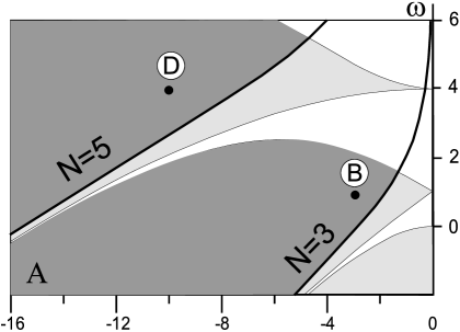
Figure 5: The plane of parameters $(\omega,A)$ with band and gap zones. The boundaries of the regions where ${\cal U}_{\pi}$ is disjoined in three (the curve $N=3$) or five (the curve $N=5$) connected components are shown. These components are islands (in the sense of Sect.3) if $\omega$ and $A$ belong to the dark zones between the marked curves and upper boundaries of the corresponding gaps.

5.2 Hypothesis 2

Since the potential $U(x)$ is even and ${\cal U}^{+}_{\pi}$ and ${\cal U}^{-}_{\pi}$ are infinite curvilinear strips, the verification of Hypothesis 2 can be fulfilled using Theorem 4.1. To this end the calculation of the values of $g_{1}(p)$ and $g_{2}(p)$ was incorporated into the procedure of the numerical scanning 1 described above. To confirm the results we also used direct visualization of the vectors $DT_{p}{\bf e}_{1,2}$ for various $p\in{\cal U}_{\pi}$.

Let us describe in detail the case $\omega=1$, $A=-2$ which is typical of the grey zone situated in the first gap, see Fig.5. The set ${\cal U}_{\pi}$ consists of three islands $D_{1}$, $D_{2}$ and $D_{3}$, see Fig.6. Their pre-images $T^{-1}D_{1}$, $T^{-1}D_{2}$ and $T^{-1}D_{3}$ intersect $D_{1}$, $D_{2}$ and $D_{3}$. Fig.6 shows the signs of $g_{1,2}(p)$ for all the intersections $T^{-1}D_{i}\cap D_{j}$, $i,j=1,2,3$. The boundaries $\beta^{\pm}_{1,2,3}$ of the islands are marked by bold dash lines. In the islands $D_{1}$ and $D_{3}$ the boundaries $\beta^{\pm}_{1,3}$ are graphs of increasing functions whereas for $D_{2}$ the boundaries $\beta^{\pm}_{2}$ are graphs of decreasing functions. It follows from Fig.6 that the signs of $g_{1,2}(p)$ conform the Hypothesis 2.

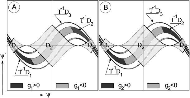
Figure 6: The region of the plane $(\psi,\psi^{\prime})$, $-1.5<\psi<1.5$, $-1.5<\psi<1.5$ with the sets ${\cal U}_{\pi}$ and $T^{-1}{\cal U}_{\pi}$, $\omega=1$, $A=-2$. The set ${\cal U}_{\pi}$ consists of three islands $D_{1}$, $D_{2}$ and $D_{3}$, the boundaries $\beta^{\pm}_{1,2,3}$ of the islands are marked by bold dash lines. The areas where $g_{1}(p)>0$ and $g_{1}(p)<0$ for $p\in T^{-1}D_{1,2,3}$ are indicated in panel A. Corresponding areas for $g_{2}(p)$ are shown in panel B.

Overall, the numerical study shows that Hypothesis 2, as well as Hypothesis 1, holds for $\omega$ and $A$ lying in the dark areas in Fig.5.

5.3 Hypothesis 3

The behavior of $\mu(\Delta_{n}^{+})$, $n=1,2,\ldots$, for various values of parameters $\omega$ and $A$ was also studied numerically. Some of the results are depicted in Fig.7.

It follows from Fig.7 that Hypothesis 3 is valid not for all the cases under consideration. A natural obstruction for Hypothesis 3 to hold is presence of elliptic fixed points or cycles. Due to KAM theory, in vicinity of an elliptic fixed point (or cycle) there exists a set of positive measure that consists of points which remain in this vicinity after any number of iterations of $T$. This means that Hypothesis 3 is not valid if the point $(\omega,A)$ is situated in a band in the plane of parameters (see Sect.5.1), because in this case the point $O(0,0)$ is an elliptic fixed point of $T$. This situation takes place for the case 1, $\omega=1$ and $A=-0.7$, in Fig.7.

As the point $(\omega,A)$ crosses a lower boundary of a gap in the plane of parameters, the point $O(0,0)$ becomes a hyperbolic fixed point and a pair of elliptic 2-cycles appears. It have been observed that this bifurcation is the first bifurcation in a cascade of period doubling bifurcations. Each of the bifurcations of this cascade gives birth to elliptic cycles of double period. Omitting the details, we summarize that the gap zones in the plane $(\omega,A)$ also contain areas where Hypothesis 3 is not valid due to presence of the elliptic cycles.

At the same time, if the point $(\omega,A)$ is situated in the dark zones in Fig.5, numerical results show that Hypothesis 3 holds. Moreover, our results allow to suppose exponential convergence of $\mu(\Delta_{n}^{+})$ to zero. The ratios $R_{n}=\mu(\Delta_{n+1}^{+})/\mu(\Delta_{n}^{+})$ are shown in panel B of Fig.7. For the cases 2 and 3, these ratios are smaller then 1 and remain close to the value $\mu(T{\cal U}_{\pi}\cap{\cal U}_{\pi})/\mu({\cal U}_{\pi})$.

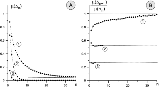
Figure 7: Panel (A): The area of the set $\Delta_{n}^{+}$ versus $n$ for $\omega=1$ and (1) $A=-0.7$, (2) $A=-1.2$ and (3) $A=-2$. Panel (B): The ratio $R_{n}=\mu(\Delta_{n+1}^{+})/\mu(\Delta_{n}^{+})$ for the same values of $\omega$ and $A$. Only few points are shown in panel (B) for the cases (2) and (3) since accuracy of calculations drastically falls due to division of small numbers.

To summarize, basing on the numerical results presented above one can conclude that if $\omega$ and $A$ are situated in the dark zones of the parameter plane, see Fig.5, the conditions of Hypotheses 1-3 hold. Therefore for these values of parameters all the nonlinear states of GPE with cosine potential can be put in one-to-one correspondence with codes from $\Omega^{N}$. When crossing the lower boundary of the grey zones (marked $N=3$ or $N=5$ in Fig.5) the conditions of Hypotheses 1 fail whereas other two Hypotheses remain valid.

5.4 More details about the map $T$

Let us describe in more detail the transformation of the sets ${\cal U}_{\pi}^{+}$ and ${\cal U}_{\pi}$ by the map $T$.

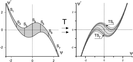
Figure 8: The action of $T$ on ${\cal U}_{\pi}^{+}$, $\omega=1$, $A=-1.5$. Vertical sections $S_{k}$, $k=1\div 7$ of ${\cal U}_{\pi}^{+}$ are mapped into the infinite curves shown in the right panel.

The action of $T$ on vertical sections of ${\cal U}_{\pi}^{+}$ is shown in Fig.8. Note that $T{\cal U}_{\pi}^{+}={\cal U}_{\pi}^{-}=I{\cal U}_{\pi}^{+}$ where $I$ is the reflection with respect to $\psi$ axis. Fig.9 illustrates the mapping of ${\cal U}_{\pi}^{+}$ and the islands $D_{1}$, $D_{2}$, $D_{3}$ (the shape of ${\cal U}_{\pi}^{+}$ was calculated for $\omega=1$, $A=-3$). It is practical to represent the map $T$ as a composition of three transformations: ${\cal U}_{\pi}^{+}\to S_{1}\to S_{2}\to{\cal U}_{\pi}^{-}$, where $S_{1}$ is an infinite horizontal strip and $S_{2}$ is an infinite vertical strip, see Fig.9. The “boundaries” $\beta^{\pm}$ of both, ${\cal U}_{\pi}^{+}$ and $S_{1}$, are in infinity. The transformation ${\cal U}_{\pi}^{+}\to S_{1}$ is a deformation. The transformation of $S_{1}$ to $S_{2}$ consists in stretching of $S_{1}$ in one dimension and contraction in another in such a way that the boundaries $\beta^{\pm}$ transform into vertical lines but $\alpha^{\pm}$ go to infinity. The transformation $S_{2}\to{\cal U}_{\pi}^{-}$ is again a deformation. As a result, $T$ maps the islands $D_{1}$, $D_{2}$, $D_{3}$ into infinite curvilinear strips. Each of these strips crosses the islands $D_{1}$, $D_{2}$, $D_{3}$ and each of the intersections is a v-strip.

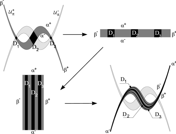
Figure 9: The action of the map $T$ on ${\cal U}_{\pi}^{+}$ and the islands $D_{1}$, $D_{2}$, $D_{3}$ (the islands and their images are indicated by the same letters). The map $T$ can be regarded as a composition of three transformations: ${\cal U}_{\pi}^{+}\to S_{1}\to S_{2}\to{\cal U}_{\pi}^{-}$: (i) deformation of ${\cal U}_{\pi}^{+}$ into infinite strip $S_{1}$, the “boundaries” $\beta^{\pm}$ of both, ${\cal U}_{\pi}^{+}$ and $S_{1}$, are in infinity; (ii) stretching of $S_{1}$ in one dimension and contraction in another one to get an infinite strip $S_{2}$, the boundaries $\beta^{\pm}$ become vertical lines but $\alpha^{\pm}$ go to infinity; (iii) deformation of $S_{2}$ into ${\cal U}_{\pi}^{-}$. As a result, $T$ maps the islands $D_{1}$, $D_{2}$, $D_{3}$ into infinite curvilinear strips. Each of these strips crosses again the islands $D_{1}$, $D_{2}$, $D_{3}$ and each of the intersections is a v-strip. The shape of ${\cal U}_{\pi}^{+}$ was calculated for $\omega=1$, $A=-3$.

An interesting issue is the study of ordering of the v-strips in ${\cal U}_{\pi}^{+}$ and the h-strips in ${\cal U}_{\pi}^{-}$ corresponding to codes with coinciding blocks. The understanding of the strip ordering is also of practical usage, since it explains the order of the nonlinear modes as they appear in shooting procedure, see Sect.5.5. We describe the ordering of v-strips, the ordering of h-strips is similar. Assume that ${\cal U}_{\pi}$ consists of $N$ disjoined islands and $N$ is odd. Consider orbits that visit the islands $D_{i_{-n}},D_{i_{-n+1}},\ldots,D_{i_{0}}$, in the given order. The points in $D_{i_{0}}$ which has this “prehistory” are situated in a strip $V_{i_{-n}i_{-n+1}\ldots i_{-2}i_{-1}i_{0}}$ constructed by the following recurrence rule

$$V_{i_{-n}i_{-n+1}}=TD_{i_{-n}}\cap D_{i_{-n+1}}$$

$$\ldots$$

$$V_{i_{-n}i_{-n+1}\ldots i_{-2}i_{-1}i_{0}}=TV_{i_{-n}i_{-n+1}\ldots i_{-2}i_{-1}}\cap D_{i_{0}}.$$

and (see C)

$$\ldots\subset V_{i_{-n}i_{-n+1}\ldots i_{-2}i_{-1}i_{0}}\subset V_{i_{-n+1}\ldots i_{-2}i_{-1}i_{0}}\subset\ldots\subset V_{i_{-2}i_{-1}i_{0}}\subset V_{i_{-1}i_{0}}\subset D_{i_{0}}$$

The orbit of a point $p\in V_{i_{-n}i_{-n+1}\ldots i_{-2}i_{-1}i_{0}}$ has in its code a block

$$(\ldots\underbrace{i_{-n}i_{-n+1}\ldots i_{-2}i_{-1}i_{0}}\ldots).$$

Since each of $i_{k}$ can take the values $1,\ldots,N$, there are $N^{n+1}$ strips in ${\cal U}_{\pi}^{+}$ each coded by the sequence of length $n+1$. The algorithm for their ordering in ${\cal U}_{\pi}^{+}$ follows immediately from geometrical properties of the intersection of the strips ${\cal U}_{\pi}^{-}$ and ${\cal U}_{\pi}^{+}$. It can be described as follows:

1. Mark the islands $D_{1}$, $\ldots$, $D_{N}$ as they are ordered in ${\cal U}_{\pi}^{+}$, see Fig.10. Draw an arrow $I_{0}$ over all of them pointing from $D_{1}$ to $D_{N}$.

2. Draw arrows $I_{01},\ldots,I_{0N}$ over each island in such a way that the directions of rightmost $I_{01}$ and leftmost $I_{0N}$ arrows coincided with the direction of $I_{0}$, but the directions of any two neighboring arrows were opposite. Sketch v-strips in $D_{i_{0}}$ in such a way that their ordering (from $V_{1i_{0}}$ to $V_{Ni_{0}}$) agreed with the direction of the arrow $I_{0i_{0}}$.

3. Draw an arrows over each of $V_{i_{-1}i_{0}}$ by the same manner and sketch v-strips $V_{i_{-2}i_{-1}i_{0}}$ according the directions of these arrows, etc.

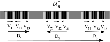
Figure 10: Algorithm for ordering of v-strips in ${\cal U}_{\pi}^{+}$.

It turns out that the algorithm given above is similar to procedure of ordering of localized modes for DNLS described in [25].

5.5 Examples

Let the parameters $(\omega,A)$ belong to the dark zone in the first gap, see Fig.5. Then all the bounded in $\mathbb{R}$ solutions of Eq.(9) can be coded by bi-infinite sequences of three symbol “alphabet”. Conversely, for each bi-infinite “word” composed by symbols of this “alphabet” these exists a solution with corresponding code. The symbols may be chosen as “$-$”, “$0$” and “$+$”, and they mark entering of the orbit into $D_{1}$, $D_{2}$ and $D_{3}$ respectively.

Example 1. Localized modes described by Eq.(9) correspond to the codes with finite numbers of nonzero symbols. In particular, Eq.(9) admits well-known solution in the form of bright gap-soliton, $\psi(x)$, [7, 9], localized in one well of the potential, see Fig.11 A. This solution corresponds to the code $(\ldots 00+00\ldots)$. Also there exist the gap soliton solution $-\psi(x)$ with the code $(\ldots 00-00\ldots)$.

Example 2. There exist exactly two $\pi$-periodic solutions of Eq.(9) with the codes $(\ldots+++\ldots)$ and $(\ldots---\ldots)$, related to each other by symmetry $\psi\to-\psi$, see Fig.11 B.

Example 3. There exists dark soliton solution of Eq.(9) corresponding to the code $(\ldots---+++\ldots)$, see Fig.11 C. Also the coding predicts that there exist other solutions of this type, having the codes $(\ldots---0+++\ldots)$, $(\ldots---00+++\ldots)$, etc.

Example 4. There exist “domain wall”-type solutions corresponding to the codes $(\ldots 000+++\ldots)$, $(\ldots---000\ldots)$. These objects were found to exist in the case of GPE with attractive nonlinearity [12]. The coding approach predicts their existence in the case of repulsive nonlinearity also. They have been found numerically, see Fig. 11 D.

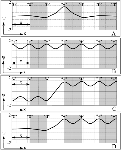
Figure 11: Nonlinear states for GPE, $\omega=1$, $A=-2$: A: bright gap-soliton, the code $(\ldots 00+00\ldots)$; B: $\pi$-periodic structure, the code $(\ldots+++\ldots)$; C: dark soliton, the code $(\ldots---+++\ldots)$; D: domain wall, the code $(\ldots 000+++\ldots)$.

Example 5. Consider boundary value problem for Eq.(9) on the interval $[-4\pi,0]$ with Neumann boundary conditions at $x=-4\pi$ and $x=0$. These solutions can be viewed as reductions to the interval of length $4\pi$ of periodic solutions with period $8\pi$ which satisfy additional symmetry conditions

$$u(x)=u(-x);\quad u(-4\pi+x)=u(-4\pi-x).$$

The codes for these solutions are of the form

$$(\ldots\theta_{5}\theta_{4}\theta_{3}\theta_{2}\underbrace{\theta_{1}\theta_{2}\theta_{3}\theta_{4}\theta_{5}\theta_{4}\theta_{3}\theta_{2}}_{\mbox{the period}}\theta_{1}\theta_{2}\theta_{3}\theta_{4}\theta_{5}\ldots),$$

where $\theta_{i}$, $i=1\div 5$, is one of the symbols “$+$”, “$0$” or “$-$”. Therefore there are $3^{5}=243$ solutions of this type. In Fig.12 nine of these solutions are depicted for $A=-2$, $\omega=1$. From numerical viewpoint, these nonlinear modes can be found by shooting method taking initial data $\psi(-4\pi)=\tilde{\psi}$, $\psi_{x}(-4\pi)=0$ and adjusting $\tilde{\psi}$ in such a way that $\psi_{x}(0)=0$. As $\tilde{\psi}$ increases, one gets the nonlinear modes one by one in the order described in Sect.5.4.

All the solutions shown in Fig.12 have the codes with $\theta_{1}=\theta_{5}=$“$0$”. Therefore they can be viewed as approximations for localized modes which have the domain of localization of length $4\pi$. These localized modes correspond to the codes

$$(\ldots 00~{}\theta_{2}\theta_{3}\theta_{4}~{}00\ldots).$$

There are $3^{3}=27$ sequences of this type but only 10 of them (including one which consists of zeroes only and corresponds to the zero solution) are different in the sense that they are not related to each other by symmetry reductions. Fig.12 shows just these nine nonzero solutions.

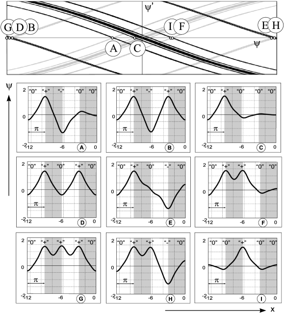
Figure 12: The solutions of Eq.(9) ($A=-2$, $\omega=1$) on the interval $[-4\pi,0]$ with Neumann boundary conditions at $x=-4\pi$ and $x=0$ (nine panels below) and the position of corresponding points in the intersection of ${\cal U}_{4\pi}^{+}$ and ${\cal U}_{4\pi}^{-}$ (upper panel). The upper panel represents the scaled rectangle marked in panel D of Fig.3 with fragments of ${\cal U}_{4\pi}^{-}$ (in black) and ${\cal U}_{4\pi}^{+}$ (in grey). The codes (the blocks $(\theta_{1}\theta_{2}\theta_{3}\theta_{4}\theta_{5})$) are: A: $(0+-00)$; B: $(0+-+0)$; C: $(0+000)$; D: $(0+0+0)$; E: $(0+0-0)$; F: $(0++00)$; G: $(0+++0)$; H: $(0++-0)$; I: $(00+00)$.

6 Conclusion

In this paper, we describe the method for coding of nonlinear states covered by 1D Gross-Pitaevskii equation with periodic potential $U(x)$ and repulsive nonlinearity. We prove that under certain conditions there exists one-to-one correspondence between the set of all bounded in $\mathbb{R}$ solutions of Eq.(6) and the set of bi-infinite sequences of numbers $1,\ldots,N$. These sequences can be regarded as codes for the solutions of Eq.(6). The number $N$ is determined by the parameters of Eq.(6). It is important that (i) each coding sequence corresponds to one and only one solution and (ii) each solutions has corresponding code. The conditions for the coding to be possible are presented in a form of three hypotheses. For a given $U(x)$, the hypotheses should be verified numerically. We report on numerical check of these hypotheses for the case of cosine potential, i.e., for Eq.(9), and indicate the regions in the plane of parameters $(\omega,A)$ where the coding is possible.

Heuristically, the coding technique described above can be interpreted as follows. The periodic potential can be regarded as an infinite chain of equidistantly spaced potential wells. It is known that if $U(x)$ is a “deep enough” single-well potential, Eq.(6) admits one or more localized solutions called “fundamental gap soliton”, FGS, in [14, 15]. Also Eq.(6) admits zero state. Assume that in total there exist $N$ states (including zero state) described by the single well potential. Note that the number $N$ is odd: since the nonlinearity is odd if $\psi(x)$ is a FGS then $-\psi(x)$ is also a solution Eq.(6) and the zero solution should also be taken into account. In these terms the coding means that one assigns to each of possible single-well states a number from 1 to $N$ and attributes to “bound states” of these entities situated in the wells of periodic potential bi-infinite “words” consisting of numbers from 1 to $N$. This viewpoint exploits an analogy between periodic problem and discrete problem replacing the solution on each period by a lattice node. The corresponding reduction can be made consistently and rigorously using Wannier functions technique [26] but the resulting system of discrete equations is nonlocal and quite difficult for a comprehensive study.

The approach presented in this paper may be applied to Eq.(6) with different types of the periodic potential $U(x)$. Also it may be extended in various directions. In particular, preliminary studies show that it can be applied with minor modifications to the equation

$$\psi_{xx}+(\omega-U(x))\psi+g_{1}\psi^{3}+g_{2}\psi^{5}=0.$$ (17)

where $g_{2}<0$. Eq.(17) also arises in the theory of BEC [27, 28]. The shapes of the sets ${\cal U}^{\pm}_{\pi}$ in this case are similar to ones described above for Eq.(6). Another possible extension of this approach can be made for complex nonlinear states of GPE, $\psi(x)=\rho(x)\exp\{i\phi(x)\}$. It is known [9] that the amplitude $\rho(x)$ obeys the equation

$$\rho_{xx}+(\omega-U(x))\rho-\rho^{3}-\frac{M^{2}}{\rho^{3}}=0,$$ (18)

where $M$ is an arbitrary real constant. For a given amplitude $\rho(x)$, the phase $\phi(x)$ can be found from the relation $\rho^{2}(x)\phi_{x}(x)=M$. Other possible extensions of the approach may be related to the cases when ${\cal U}_{\pi}$ consists of partially overlapping islands or of more general sets which are not islands at all.

Having in hand a complete description of nonlinear modes for Eq.(6) in terms of their codes, one can return to the problem of stability of these modes. In our opinion, a relation between the code and the stability of corresponding mode is an interesting issue for further study. A good example of such a study is paper [29] where the similar problem was considered for DNLS.

At last, let us note that the approach developed in this paper cannot be applied (at least, directly) to the case of GPE with attractive interactions, $\sigma<0$ in Eq.(4). One can prove that in this case all the solutions of Eq.(4) are non-collapsing under quite general assumptions for the potential $U(x)$.

Appendix A Proof of Theorem 2.1

The following statement proved in [17] will be used below:

Comparison Lemma. Let the functions $y(t)$ and $x(t)$, $t\in[a;b]$ be solutions of equations

$$y_{tt}-g(t,y)=0$$ (19)

$$x_{tt}-f(t,x)=0$$ (20)

correspondingly. Let also the following conditions hold:

(i) $f(t,\xi)$, $g(t,\xi)$ are defined on $[a;b]\times[A;B]$ and locally Lipschitz continuous with respect to $\xi$, $\xi\in[A;B]$, ($A$,$B$, $b$ may be finite or infinite);

(ii) $g(t,\xi)\geq f(t,\xi)$ for any $t\in[a;b]$, $\xi\in[A;B]$;

(iii) $f(t,\xi)$ is monotone nondecreasing with respect to $\xi$, $\xi\in[A;B]$.

Let $A<x(a)\leq y(a)<B$ and $x_{t}(a)\leq y_{t}(a)$. Then $x_{t}(t)\leq y_{t}(t)$ and $x(t)\leq y(t)$ while $A<x(t),y(t)<B$ or for the whole interval $t\in[a;b]$

In what follows we assume that the potential $U(x)$ be continuous and bounded on $\mathbb{R}$ and use the notations introduced in Sect.2.1. To prove Theorem 2.1 we need the following lemmas:

Lemma 2.1. Let $\psi^{\prime}_{0}\geq 0$. Then for $\psi_{0}>\sqrt{\overline{\Omega}}$

$$h^{+}(\psi_{0},\psi^{\prime}_{0})\leq h^{+}_{0}(\psi_{0})\equiv\int_{\psi_{0}}^{\infty}\frac{\sqrt{2}~{}d\eta}{\sqrt{\eta^{4}-\psi_{0}^{4}-2\overline{\Omega}(\eta^{2}-\psi_{0}^{2})}},$$ (21)

and $h^{+}_{0}(\psi_{0})\sim\frac{{\rm K}(1/\sqrt{2})}{\psi_{0}}$ when $\psi_{0}\to+\infty$. Here ${\rm K}(\cdot)$ is complete elliptic integral of the first kind.

Proof: Consider the equation

$$\phi_{xx}+\overline{\Omega}\phi-\phi^{3}=0$$ (22)

The solution $\phi(x)$ for Eq.(22) with initial data $\phi(0)=\psi_{0}$, $\phi_{x}(0)=\psi_{0}^{\prime}$ can be written in implicit form as follows

$$x=\int_{\psi_{0}}^{\phi}\frac{\sqrt{2}~{}d\eta}{\sqrt{\Delta-2\overline{\Omega}\eta^{2}+\eta^{4}}};\quad\Delta=2(\psi_{0}^{\prime})^{2}+2\overline{\Omega}\psi_{0}^{2}-\psi_{0}^{4}.$$ (23)

The solution $\phi(x)$ tends to $+\infty$ at the point

$$x_{0}=\int_{\psi_{0}}^{\infty}\frac{\sqrt{2}~{}d\eta}{\sqrt{\eta^{4}-\psi_{0}^{4}-2\overline{\Omega}(\eta^{2}-\psi_{0}^{2})+2(\psi_{0}^{\prime})^{2}}}$$

and the following estimation holds

$$x_{0}\leq h^{+}(\psi_{0})\equiv\int_{\psi_{0}}^{\infty}\frac{\sqrt{2}~{}d\eta}{\sqrt{\eta^{4}-\psi_{0}^{4}-2\overline{\Omega}(\eta^{2}-\psi_{0}^{2})}}\sim\frac{{\rm K}(1/\sqrt{2})}{\psi_{0}},\quad\psi_{0}\to+\infty$$

Now let us consider the solution $\psi(x)$ of Eq.(6) with initial data $\psi(0)=\psi_{0}$, $\psi_{x}(0)=\psi_{0}^{\prime}$. Since for $\xi>\sqrt{\overline{\Omega}}$ the function $F(\xi)=\xi^{3}-\overline{\Omega}\xi$ is monotonic and $\xi^{3}-(\omega-U(x))\xi\geq F(\xi)$ one can apply Comparison Lemma from [17] to Eq.(6) and Eq.(22). Therefore for $x>0$ the inequality $\psi(x)\geq\phi(x)$ holds. This means that $\psi(x)$ collapses at a point $h^{+}(\psi_{0},\psi^{\prime}_{0})\leq x_{0}\leq h^{+}_{0}(\psi_{0})$. This proves Lemma 2.1. $\blacksquare$

Lemma 2.2. For each $L$ there exists a value $\tilde{\psi}_{L}$ such that the set ${\cal U}_{L}$ is situated in the plane $\mathbb{R}^{2}=(\psi,\psi^{\prime})$ in the strip $-\tilde{\psi}_{L}<\psi<\tilde{\psi}_{L}$.

Proof: Due to Lemma 2.1 for each $L$ there exists $\tilde{\psi}_{L}$ such that there are no points of ${\cal U}_{L}$ in the sector $\psi>\tilde{\psi}_{L}$, $\psi^{\prime}\geq 0$. Since Eq.(6) is invariant with respect to the symmetry $\psi\to-\psi$ the estimation (21) holds also for $\psi^{\prime}_{0}\leq 0$ and $\psi_{0}<-\sqrt{\overline{\Omega}}$, therefore there are no points of ${\cal U}_{L}$ in the sector $\psi<-\tilde{\psi}_{L}$, $\psi^{\prime}\leq 0$. Making the transformation $x\to-x$ and repeating the reasoning of Lemma 2.1 we obtain the estimation

$$h^{-}(\psi_{0},\psi^{\prime}_{0})\leq h^{-}_{0}(\psi_{0})\equiv\int_{-\infty}^{\psi_{0}}\frac{\sqrt{2}~{}d\eta}{\sqrt{\eta^{4}-\psi_{0}^{4}-2\overline{\Omega}(\eta^{2}-\psi_{0}^{2})}}$$

for the two cases: (i) $\psi_{0}>\sqrt{\overline{\Omega}}$, $\psi^{\prime}_{0}\leq 0$ and (ii) $\psi_{0}<-\sqrt{\overline{\Omega}}$, $\psi^{\prime}_{0}\geq 0$. Similarly, $h^{-}_{0}(\psi_{0})\sim-\frac{{\rm K}(1/\sqrt{2})}{\psi_{0}}$, $\psi_{0}\to-\infty$. Therefore there are no points of ${\cal U}_{L}$ in the sectors $\psi>\tilde{\psi}_{L}$, $\psi^{\prime}\leq 0$ and $\psi<-\tilde{\psi}_{L}$, $\psi^{\prime}\geq 0$. This implies the statement of Lemma 2.2. $\blacksquare$

Proof of Theorem 2.1: Due to Lemma 2.2 there exists the value $\tilde{\psi}_{L}$ such that no points of ${\cal U}_{L}$ are situated out of the strip $-\tilde{\psi}_{L}<\psi<\tilde{\psi}_{L}$. Therefore it is enough to prove that there are no points of ${\cal U}_{L}$ in two half-strips

$$S^{+}_{R}=\{(\psi,\psi^{\prime})\in\mathbb{R}^{2}|~{}-\tilde{\psi}_{L}<\psi<\tilde{\psi}_{L},~{}\psi^{\prime}>R\}$$

$$S^{-}_{R}=\{(\psi,\psi^{\prime})\in\mathbb{R}^{2}|~{}-\tilde{\psi}_{L}<\psi<\tilde{\psi}_{L},~{}\psi^{\prime}<-R\}$$

for $R$ large enough. Let us prove this fact for $S^{+}_{R}$, the proof for $S^{-}_{R}$ is analogous. It follows from Lemma 2.2 that there exists the value $\tilde{\psi}_{L/2}>\tilde{\psi}_{L}$ such that all the points $(\psi,\psi^{\prime})$ for $\psi>\tilde{\psi}_{L/2}$ and $\psi^{\prime}\geq 0$ are $L/2$-collapsing forward points. Introduce the value

$$M_{L}\equiv\min_{\begin{array}[]{c}\xi\in[-\tilde{\psi}_{L/2};\tilde{\psi}_{L/2}]\\ \eta\in[\underline{\Omega};\overline{\Omega}]\end{array}}\left(\xi^{3}-\eta\xi\right)$$

Evidently $M_{L}\leq 0$. Consider the solution $\psi(x)$ of Cauchy problem for Eq.(6) with initial data $\psi(0)=\psi_{0}$, $\psi_{0}\in[-\tilde{\psi}_{L};\tilde{\psi}_{L}]$ and $\psi_{x}(0)=\psi^{\prime}_{0}$, $\psi^{\prime}_{0}>R$. While $-\tilde{\psi}_{L/2}\leq\psi(x)\leq\tilde{\psi}_{L/2}$ one has $\psi_{xx}(x)\geq M_{L}$. Then the following relations hold

$$\psi_{x}(x)\geq\psi_{x}(0)+M_{L}x\geq R+M_{L}x,$$ (25)

$$\psi(x)\geq\psi(0)+Rx+\frac{M_{L}}{2}x^{2}\geq-\tilde{\psi}_{L}+Rx+\frac{M_{L}}{2}x^{2}.$$ (26)

We claim that if the initial data for Eq.(6) are situated in the half-strip $S^{+}_{R}$ with

$$R>\tilde{\psi}^{\prime}_{L}\equiv\max\left\{-\frac{M_{L}L}{2},\frac{1}{4L}\left(8\tilde{\psi}_{L/2}+8\tilde{\psi}_{L}-M_{L}L^{2}\right)\right\}$$

then the segment of curve $\{(\psi(x),\psi_{x}(x)),~{}0\leq x\leq L/2\}$ crosses the line $\psi=\tilde{\psi}_{L/2}$ in some point where $\psi^{\prime}\geq 0$. In fact, assuming that $-\tilde{\psi}_{L/2}\leq\psi(x)\leq\tilde{\psi}_{L/2}$ for $x\in[0;L/2]$ from (25) and (26) one concludes that

$$\psi_{x}(x) \geq R+M_{L}x>0,\quad x\in[0;L/2];$$

$$\psi(0) \leq \tilde{\psi}_{L}\leq\tilde{\psi}_{L/2};\quad\psi(L/2)\geq-\tilde{\psi}_{L}+\frac{RL}{2}+\frac{M_{L}L^{2}}{8}>\tilde{\psi}_{L/2},$$

i.e. we arrive at the contradiction. Therefore there exists a value $\tilde{x}\in[0;L/2]$ such that $\psi(\tilde{x})>\tilde{\psi}_{L/2}$ and $\psi_{x}(\tilde{x})>0$ i.e. $(\psi(\tilde{x}),\psi_{x}(\tilde{x}))$ is $L/2$-collapsing forward point. Then $(\psi(0),\psi_{x}(0))$ is $L$-collapsing forward point. So, for $R>\tilde{\psi}^{\prime}_{L}$ there are no points from ${\cal U}_{L}$ in $S^{+}_{R}$. $\blacksquare$

Appendix B Proof of Theorem 2.2

Proof of Theorem 2.2. Introduce the following functions:

(a) the function $\tilde{H}^{+}(\tilde{\psi},\tilde{\psi}^{\prime},\Omega;t)$ defined as follows: $\tilde{H}^{+}(\tilde{\psi},\tilde{\psi}^{\prime},\Omega;t)=x_{0}$ if the solution of Cauchy problem for the equation

$$\phi_{xx}+\Omega\phi-\phi^{3}=0$$

with initial data $\phi(t)=\tilde{\psi}$, $\phi_{x}(t)=\tilde{\psi}^{\prime}$ collapses at the value $x=x_{0}$, $x_{0}>0$. Exact formula for $\tilde{H}^{+}(\tilde{\psi},\tilde{\psi}^{\prime},\Omega;t)$ is

$$\tilde{H}^{+}(\tilde{\psi},\tilde{\psi}^{\prime},\Omega;t)=t+\int_{\tilde{\psi}}^{\infty}\frac{\sqrt{2}~{}d\eta}{\sqrt{\eta^{4}-\tilde{\psi}^{4}-2{\Omega}(\eta^{2}-\tilde{\psi}^{2})+2(\tilde{\psi}^{\prime})^{2}}}$$ (27)

It follows from (27) that if $\tilde{H}^{+}(\psi_{0},\psi^{\prime}_{0},\Omega_{0};t)<\infty$ then for $t$ fixed the function $H^{+}(\tilde{\psi},\tilde{\psi}^{\prime},\Omega;t)$ is a continuous function of the variables $\tilde{\psi},\tilde{\psi}^{\prime},\Omega$ in some vicinity of the point $(\psi_{0},\psi^{\prime}_{0},\Omega_{0})$.

(b) the function $\tilde{h}^{+}(\tilde{\psi},\tilde{\psi}^{\prime};t)$ defined as follows: $\tilde{h}^{+}(\tilde{\psi},\tilde{\psi}^{\prime};t)=x_{0}$ if the solution of Cauchy problem for Eq.(6) with initial data $\psi(t)=\tilde{\psi}$, $\psi_{x}(t)=\tilde{\psi}^{\prime}$ collapses at value $x=x_{0}$, $x_{0}>0$. Evidently, if $\psi(x)$ is a solution of Eq.(6) then

$$h^{+}(\psi(0),\psi_{x}(0))=\tilde{h}^{+}(\psi(t),\psi_{x}(t);t)+t$$ (28)

(c) the two functions

$$\Omega_{1}(t)=\min_{x\in[t;L]}(\omega-U(x)),\quad\Omega_{2}(t)=\max_{x\in[t;L]}(\omega-U(x))$$

which are continuous functions in some vicinity of the point $t=L$.

Also let us denote by $D_{\delta}(\zeta,\zeta^{\prime})$ a disc in $\mathbb{R}^{2}$ with center at $(\zeta,\zeta^{\prime})$ and radius $\delta$.

It follows from the conditions of Theorem 2.2 that the solution $\psi(x)$ of Eq.(6) with initial data $\psi(0)=\psi_{0}$, $\psi_{x}(0)=\psi_{0}^{\prime}$ satisfies one of the conditions

$$\lim_{x\to L}\psi(x)=+\infty,\quad\mbox{or}\quad\lim_{x\to L}\psi(x)=-\infty$$

Let the behavior of $\psi(x)$ in vicinity of $x=L$ obey the first of the two formulas above (the analysis of the second case is similar). Then there exists $t$ such that $\psi(x)>\sqrt{\Omega_{1}(t)}$ and $\psi_{x}(x)>0$ for $x\in[t;L)$. By virtue of Comparison Lemma, see A, one has

$$\tilde{H}^{+}(\tilde{\psi},\tilde{\psi}^{\prime},\Omega_{1}(t^{*});t^{*})\leq\tilde{h}^{+}(\tilde{\psi},\tilde{\psi}^{\prime};t^{*})\leq\tilde{H}^{+}(\tilde{\psi},\tilde{\psi}^{\prime},\Omega_{2}(t^{*});t^{*})$$ (29)

for any $t^{*}\in[t;L)$ and for any $\tilde{\psi},\tilde{\psi}^{\prime}$ in some vicinity of the point $(\psi(t^{*}),\psi^{\prime}(t^{*}))$.

Let us describe 3-step algorithm which allows by given $\varepsilon>0$ to find $\delta>0$ such that if $(\psi,\psi^{\prime})\in D_{\delta}(\psi_{0},\psi_{0}^{\prime})$ then

$$|h^{+}(\psi,\psi^{\prime})-h^{+}(\psi_{0},\psi_{0}^{\prime})|<\varepsilon.$$ (30)

1. By given $\varepsilon$ one can find $t^{*}$ such that the inequality holds

$$|\tilde{H}^{+}(\psi(t^{*}),\psi^{\prime}(t^{*}),\Omega_{2}(t^{*});t^{*})-\tilde{H}^{+}(\psi(t^{*}),\psi^{\prime}(t^{*}),\Omega_{1}(t^{*});t^{*})|\leq\varepsilon/2$$ (31)

2. Since $\tilde{H}^{+}(\tilde{\psi},\tilde{\psi}^{\prime},\Omega;t)$ is continuous there exists $\delta_{1}>0$ such that when $(\tilde{\psi},\tilde{\psi}^{\prime})\in D_{\delta_{1}}(\psi(t^{*}),\psi^{\prime}(t^{*}))$ the inequalities hold

$$|\tilde{H}^{+}(\tilde{\psi},\tilde{\psi}^{\prime},\Omega_{2}(t^{*});t^{*})-\tilde{H}^{+}(\psi(t^{*}),\psi^{\prime}(t^{*}),\Omega_{2}(t^{*});t^{*})|\leq\varepsilon/2$$

$$|\tilde{H}^{+}(\tilde{\psi},\tilde{\psi}^{\prime},\Omega_{1}(t^{*});t^{*})-\tilde{H}^{+}(\psi(t^{*}),\psi^{\prime}(t^{*}),\Omega_{1}(t^{*});t^{*})|\leq\varepsilon/2$$

It follows from (29) and (31) that if $(\tilde{\psi},\tilde{\psi}^{\prime})\in D_{\delta_{1}}(\psi(t^{*}),\psi^{\prime}(t^{*}))$ then

$$|\tilde{h}^{+}(\tilde{\psi},\tilde{\psi}^{\prime};t^{*})-\tilde{h}^{+}(\psi(t^{*}),\psi^{\prime}(t^{*});t^{*})|\leq\varepsilon$$ (32)

3. The flow defined by Eq.(6) generates a diffeomorphism $T_{t^{*}}:\mathbb{R}^{2}\to\mathbb{R}^{2}$ which maps a point $(\psi(t^{*}),\psi_{x}(t^{*}))$ to a point $(\psi(0),\psi_{x}(0))$ where $\psi(x)$ is a solution of Eq.(6). Then there exists $\delta$ such that $D_{\delta}(\psi_{0},\psi_{0}^{\prime})\subset T_{t^{*}}D_{\delta_{1}}(\psi(t^{*}),\psi_{x}(t^{*}))$. By means of (28) and (32) one concludes that for $(\psi,\psi^{\prime})\in D_{\delta}(\psi_{0},\psi_{0}^{\prime})$ the relation (30) holds. Theorem 2.2 is proved. $\blacksquare$

Appendix C Proof of Theorem 3.1.

Before proving Theorem 3.1 we prove the following lemma:

Lemma 3.1. Let $D$ be an island.

(i) Let $D\supset V_{1}\supset V_{2}\supset\ldots$ be an infinite sequence of nested v-strips such that

$$\lim_{n\to\infty}\mu(V_{n})=0.$$ (33)

Then the intersection

$$V_{\infty}=\bigcap_{n=1}^{\infty}V_{n}$$

is a v-curve.

(ii) Let $D\supset H_{1}\supset H_{2}\supset\ldots$ is an infinite sequence of nested h-strips and

$$\lim_{n\to\infty}\mu(H_{n})=0.$$

Then the intersection

$$H_{\infty}=\bigcap_{n=1}^{\infty}H_{n}$$

is an h-curve.

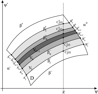
Figure 13: Illustration to the proof of Lemma 3.1.

Proof of Lemma 3.1. Let us prove the point (i), the point (ii) can be proved similarly. Denote the v-curves which bound the strip $V_{n}$ by $\beta_{n}^{-}$ (which lies closer to $\beta^{-}$) and $\beta_{n}^{+}$ (which lies closer to $\beta^{+}$). Let the endpoints of $\beta_{n}^{+}$ be $A_{n}^{+}$ (situated at $\alpha^{-}$) and $B_{n}^{+}$ (situated at $\alpha^{+}$). Let the endpoints of $\beta_{n}^{-}$ be $A_{n}^{-}$ (situated at $\alpha^{-}$) and $B_{n}^{-}$ (situated at $\alpha^{-}$), see Fig.13.

First, we show that $A_{n}^{-}\to A_{n}^{+}$ and $B_{n}^{-}\to B_{n}^{+}$ as $n\to\infty$. The sequence of points $A_{1}^{-},A_{2}^{-},\ldots$ is situated on the curve $\alpha^{-}$ from one side from the point $A_{1}^{+}$ and is “monotonic” in the sense that for any $n$ the point $A_{n+1}^{-}$ is situated on $\alpha^{-}$ between the points $A_{n}^{-}$ and $A_{1}^{+}$. Therefore it has a limit point $A_{\infty}^{+}\in\alpha^{-}$. The sequence of points $A_{1}^{+},A_{2}^{+},\ldots$ is situated on the curve $\alpha^{-}$ from one side of the point $A_{1}^{-}$ and has similar monotonic property. Therefore it also has a limit point $A_{\infty}^{-}\in\alpha^{-}$. Suppose that $A_{\infty}^{+}\neq A_{\infty}^{-}$. Then, since $\beta_{n}^{\pm}$ are graphs of monotone non-increasing/non-decreasing $\gamma$-Lipschitz functions and $\alpha^{-}$ is a graph of monotone non-decreasing/non-increasing $\gamma$-Lipschitz function, the area of $V_{n}$ cannot tend to zero as $n\to\infty$. Therefore $A_{\infty}^{+}=A_{\infty}^{-}=A_{\infty}$. In the same way one can introduce the limit points $B_{\infty}^{-}\in\alpha^{+}$ and $B_{\infty}^{+}\in\alpha^{+}$ and conclude that $B_{\infty}^{+}=B_{\infty}^{-}=B_{\infty}$.

Second, let coordinates of $A_{\infty}$ be $(\psi_{A},\psi^{\prime}_{A})$ and coordinates of $B_{\infty}$ be $(\psi_{B},\psi^{\prime}_{B})$. Consider a real value $z$ situated between $\psi_{A}$ and $\psi_{B}$. Since $A_{n}^{-}\to A_{n}^{+}$ and $B_{n}^{-}\to B_{n}^{+}$ as $n\to\infty$ there exists $n_{0}$ such that for $n>n_{0}$ both $\beta_{n}^{+}$ and $\beta_{n}^{-}$ intersect the line $\psi=z$. Denote the points of intersections of $\beta_{n}^{+}$ and $\beta_{n}^{-}$ with the line $\psi=z$ correspondingly $C_{n}^{+}(z)$ and $C_{n}^{-}(z)$. Evidently, both the sequences $\{C_{n}^{+}(z)\}$ and $\{C_{n}^{-}(z)\}$ have limits as $n\to\infty$. Denote these limits $C^{+}(z)$ and $C^{-}(z)$ correspondingly.

Assume that at some $z=z^{*}$ one has $|C^{+}(z)-C^{-}(z)|=\delta_{C}>0$. The relation $C^{+}(z)\neq C^{-}(z)$ cannot hold in some vicinity of the point $z=z^{*}$, otherwise there exists a set of nonzero measure which belongs to all the nested strips $V_{n}$ and $\mu(V_{n})$ does not tend to zero as $n\to\infty$. Therefore for any $\varepsilon$ there exist a value $z_{1}$, such that $|z_{1}-z^{*}|<\varepsilon$ and $C^{+}(z_{1})=C^{-}(z_{1})$. This means that (al least) one of the ratios

$$\frac{|C^{+}(z_{1})-C^{+}(z^{*})|}{|z_{1}-z^{*}|},\quad\frac{|C^{-}(z_{1})-C^{-}(z^{*})|}{|z_{1}-z^{*}|}$$

is greater than $\delta_{C}/2\varepsilon$. Since $\varepsilon$ can be taken arbitrarily small, this contradicts the condition that $\beta_{n}^{\pm}$ are graphs of monotone non-increasing/non-decreasing $\gamma$-Lipschitz functions. This implies that $C^{+}(z)=C^{-}(z)\equiv C(z)$ for all $z$, $\psi_{A}<z<\psi_{B}$.

Third, each of the curves $\beta_{n}^{-}$ is a graph of a monotone non-increasing/non-decreasing $\gamma$-Lipschitz function. Passing to the limit $n\to\infty$ we obtain a curve consisting of the points $C(z)$, $\psi_{A}<z<\psi_{B}$. This curve is also a graph of monotone non-increasing/non-decreasing $\gamma$-Lipschitz function with the same $\gamma$, (see [22], Sect 4.3), i.e. v-curve.$\blacksquare$

Proof of Theorem 3.1. Evidently, for each ${\bf p}\in{\cal P}$ the image ${\bf s}=\Sigma{\bf p}\in\Omega^{N}$ is defined uniquely. Let us prove that for each ${\bf s}\in\Omega^{N}$ there exists unique ${\bf p}\in{\cal P}$ such that ${\bf s}=\Sigma{\bf p}$. Consider a sequence ${\bf s}=\{\ldots,i_{-1},i_{0},i_{1},\ldots\}$, $i_{k}\in\{1,\ldots,N\}$. Let us find the location of the points $p\in D_{i_{0}}$ such that $T^{-1}p\in D_{i_{-1}}$, $T^{-2}p\in D_{i_{-2}}$ etc. It is easy to check that:

- the points $p\in D_{i_{0}}$ such that $T^{-1}p\in D_{i_{-1}}$ are situated in the set $V_{i_{-1}i_{0}}=TD_{i_{-1}}\cap D_{i_{0}}$. Due to the condition (i) of theorem, $V_{i_{-1}i_{0}}$ is a v-strip. Moreover, $V_{ji_{0}}$ and $V_{ki_{0}}$ have no common points if $j\neq k$.

- the points $q\in D_{i_{-1}}$ such that $T^{-1}q\in D_{i_{-2}}$ are situated in the set $V_{i_{-2}i_{-1}}=TD_{i_{-2}}\cap D_{i_{-1}}$ which is a v-strip. The points $p\in D_{i_{0}}$ such that $T^{-1}p=q\in D_{i_{-1}}$, $T^{-2}p=T^{-1}q\in D_{i_{-2}}$ are situated in the set $V_{i_{-2}i_{-1}i_{0}}=TV_{i_{-2}i_{-1}}\cap D_{i_{0}}$ which is also v-strip. Evidently, $V_{i_{-2}i_{-1}i_{0}}\subset V_{i_{-1}i_{0}}$. Also, $V_{ji_{-1}i_{0}}$ and $V_{ki_{-1}i_{0}}$ have no common points if $j\neq k$.

Continuing the process, we have nested sequence of v-strips

$$\ldots V_{i_{-(n+1)}i_{-n}\ldots i_{-2}i_{-1}i_{0}}\subset V_{i_{-n}\ldots i_{-2}i_{-1}i_{0}}\subset\ldots\subset V_{i_{-2}i_{-1}i_{0}}\subset V_{i_{-1}i_{0}}\subset D_{i_{0}}$$

such that $V_{i_{-(n+1)}i_{-n}\ldots i_{-2}i_{-1}i_{0}}=TV_{i_{-(n+1)}i_{-n}\ldots i_{-2}i_{-1}}\cap D_{i_{0}}$. Since

$$\mu(V_{i_{-n}\ldots i_{-2}i_{-1}i_{0}})\leq\mu(\Delta^{+}_{n})$$

the area of v-strip $V_{i_{-n}\ldots i_{-2}i_{-1}i_{0}}$ tends to zero as $n\to\infty$. According to Lemma 3.1 the intersection of these nested strips, $V_{\infty}$, exists and is a v-curve.

In the same manner the nested sequence of h-strips can be constructed,

$$\ldots H_{i_{0}i_{1}\ldots i_{n}i_{n+1}}\subset H_{i_{0}i_{1}\ldots i_{n}}\subset\ldots\subset H_{i_{0}i_{1}i_{2}}\subset H_{i_{0}i_{1}}\subset D_{i_{0}}$$

where $H_{i_{0}i_{1}\ldots i_{n}i_{n+1}}=T^{-1}H_{i_{0}i_{1}\ldots i_{n}}\cap D_{i_{0}}$. The area of the strip $H_{i_{0}i_{1}\ldots i_{n}}$ tends to zero as $n\to\infty$ so according to Lemma 3.1 the intersection of these nested strips, $H_{\infty}$, exists and is an h-curve.

The orbit ${\bf p}\in{\cal P}$ corresponding to bi-infinite sequence ${\bf s}=\{\ldots,i_{-1},i_{0},i_{1},\ldots\}$ is generated by $T$- and $T^{-1}$-iterations of the intersection $H_{\infty}\cap V_{\infty}$ which according to the definition of h- and v-curves consists of one point. Therefore ${\bf p}$ exists and is unique.

The continuity of $\Sigma$ and $\Sigma^{-1}$ follows from the following observations:

- since $T$ is continuous, if ${\bf p}^{(1)}=\{\ldots,p_{-1}^{(1)},p_{0}^{(1)},p_{1}^{(1)},\ldots\}$ and ${\bf p}^{(2)}=\{\ldots,p_{-1}^{(2)},p_{0}^{(2)},p_{1}^{(2)},\ldots\}$ are close enough in ${\cal P}$ (i.e. the points $p_{0}^{(1)}$ and $p_{0}^{(2)}$ are close in $\mathbb{R}^{2}$), then their $\Sigma$-images share the same central block $|i|<k$ for some $k$. Therefore they are also close in $\Omega^{N}$-topology;

- if ${\bf s}^{(1)}=\Sigma{\bf p}^{(1)}$ and ${\bf s}^{(2)}=\Sigma{\bf p}^{(2)}$ share the same central block $|i|<k$ for some $k$, the points $p_{0}^{(1)}$ and $p_{0}^{(2)}$ are situated in the curvilinear quadrangle $V_{i_{-k}\ldots i_{-2}i_{-1}i_{0}}\cap H_{i_{0}i_{1}\ldots i_{k}}$, so ${\bf p}^{(1)}$ and ${\bf p}^{(2)}$ are close in ${\cal P}$-topology. $\blacksquare$

Appendix D Proof of Theorem 4.1

Let ${\bf e}_{1,2}$ be unit vectors (15). Denfine the following cones

$$\mathbb{R}^{2}_{++}=\{{\bf a}|~{}{\bf a}=x{\bf e}_{1}+y{\bf e}_{2},~{}x>0,y>0\},$$

$$\overline{\mathbb{R}}^{2}_{++}=\{{\bf a}|~{}{\bf a}=x{\bf e}_{1}+y{\bf e}_{2},~{}x\geq 0,y\geq 0\},$$

$$\mathbb{R}^{2}_{-+}=\{{\bf a}|~{}{\bf a}=x{\bf e}_{1}+y{\bf e}_{2},~{}x>0,y<0\},$$

$$\overline{\mathbb{R}}^{2}_{-+}=\{{\bf a}|~{}{\bf a}=x{\bf e}_{1}+y{\bf e}_{2},~{}x\geq 0,y\leq 0\},$$

$$\mathbb{R}^{2}_{+-}=\{{\bf a}|~{}{\bf a}=x{\bf e}_{1}+y{\bf e}_{2},~{}x>0,y<0\},$$

$$\overline{\mathbb{R}}^{2}_{+-}=\{{\bf a}|~{}{\bf a}=x{\bf e}_{1}+y{\bf e}_{2},~{}x\geq 0,y\leq 0\},$$

$$\mathbb{R}^{2}_{--}=\{{\bf a}|~{}{\bf a}=x{\bf e}_{1}+y{\bf e}_{2},~{}x<0,y<0\},$$

$$\overline{\mathbb{R}}^{2}_{--}=\{{\bf a}|~{}{\bf a}=x{\bf e}_{1}+y{\bf e}_{2},~{}x\leq 0,y\leq 0\}.$$

Lemma 4.1. Let $S\subset{\mathbb{R}}^{2}$ be a compact connected set, $T$ be a diffeomorphism defined on $S$, the operator $DT_{p}$ be nondegenerate for all $p\in S$ and ${\bf e}_{1}$,${\bf e}_{2}$ be the unit vectors defined by (15).

I. Let for all $p\in S$ the relations $g_{1}(p)>0$ and $g_{2}(p)>0$ hold. Then

a. For all $p\in S$ one and only one of the following alternative conditions holds

$${\rm[A1]} ~{}DT_{p}[\overline{\mathbb{R}}^{2}_{++}]\subset\mathbb{R}^{2}_{++};\quad{\rm[A2]}~{}DT_{p}[\overline{\mathbb{R}}^{2}_{++}]\subset\mathbb{R}^{2}_{--};$$

$${\rm[A3]} ~{}DT_{p}[\overline{\mathbb{R}}^{2}_{++}]\subset\mathbb{R}^{2}_{+-};\quad{\rm[A4]}~{}DT_{p}[\overline{\mathbb{R}}^{2}_{++}]\subset\mathbb{R}^{2}_{-+}$$

b. there exists $\gamma>0$ such that for any two points $p_{1}=(\psi_{1},\psi_{1}^{\prime})\in S$ and $p_{2}=(\psi_{2},\psi_{2}^{\prime})\in S$, $\psi_{1}<\psi_{2}$ and $\psi^{\prime}_{1}<\psi^{\prime}_{2}$ the images $Tp_{1}=q_{1}=(\phi_{1},\phi_{1}^{\prime})$, $Tp_{2}=q_{2}=(\phi_{2},\phi_{2}^{\prime})$ are such that

$$\mbox{in the case [A1]}:\quad 0<\phi_{2}-\phi_{1}<\gamma(\phi^{\prime}_{2}-\phi^{\prime}_{1})$$

$$\mbox{in the case [A2]}:\quad 0<\phi_{1}-\phi_{2}<\gamma(\phi^{\prime}_{1}-\phi^{\prime}_{2})$$

$$\mbox{in the case [A3]}:\quad 0<\phi_{1}-\phi_{2}<\gamma(\phi^{\prime}_{2}-\phi^{\prime}_{1})$$

$$\mbox{in the case [A4]}:\quad 0<\phi_{2}-\phi_{1}<\gamma(\phi^{\prime}_{1}-\phi^{\prime}_{2})$$

II. Let for all $p\in S$ the relations $g_{1}(p)<0$ and $g_{2}(p)<0$ hold. Then

a. For all $p\in S$ one and only one of the following alternative conditions holds

$${\rm[B1]} ~{}DT_{p}[\overline{\mathbb{R}}^{2}_{-+}]\subset\mathbb{R}^{2}_{++};\quad{\rm[B2]}~{}DT_{p}[\overline{\mathbb{R}}^{2}_{-+}]\subset\mathbb{R}^{2}_{--};$$

$${\rm[B3]} ~{}DT_{p}[\overline{\mathbb{R}}^{2}_{-+}]\subset\mathbb{R}^{2}_{+-};\quad{\rm[B4]}~{}DT_{p}[\overline{\mathbb{R}}^{2}_{-+}]\subset\mathbb{R}^{2}_{-+}$$

b. There exists $\gamma>0$ such that for any two points $p_{1}=(\psi_{1},\psi_{1}^{\prime})\in S$ and $p_{2}=(\psi_{2},\psi_{2}^{\prime})\in S$, $\psi_{1}<\psi_{2}$ and $\psi^{\prime}_{1}>\psi^{\prime}_{2}$ the images $Tp_{1}=q_{1}=(\phi_{1},\phi_{1}^{\prime})$, $Tp_{2}=q_{2}=(\phi_{2},\phi_{2}^{\prime})$ are such that

$$\mbox{in the case [B1]}:\quad 0<\phi_{2}-\phi_{1}<\gamma(\phi^{\prime}_{2}-\phi^{\prime}_{1})$$

$$\mbox{in the case [B2]}:\quad 0<\phi_{1}-\phi_{2}<\gamma(\phi^{\prime}_{1}-\phi^{\prime}_{2})$$

$$\mbox{in the case [B3]}:\quad 0<\phi_{1}-\phi_{2}<\gamma(\phi^{\prime}_{2}-\phi^{\prime}_{1})$$

$$\mbox{in the case [B4]}:\quad 0<\phi_{2}-\phi_{1}<\gamma(\phi^{\prime}_{1}-\phi^{\prime}_{2})$$

Proof of Lemma 4.1. Let us prove the point Ia, the point IIa can be proved similarly. Evidently, the relations $g_{1}(p)>0$ and $g_{2}(p)>0$ mean that both the vectors $DT_{p}{\bf e}_{1}$, $DT_{p}{\bf e}_{2}$ are situated in the same quadrant, $\mathbb{R}^{2}_{++}$, $\mathbb{R}^{2}_{-+}$, $\mathbb{R}^{2}_{+-}$ or $\mathbb{R}^{2}_{--}$ for any $p\in S$. Let for two points $p_{1}$ and $p_{2}$ these quadrants are different. Connect these points by continuous curve $\zeta\subset S$. Since $DT_{p}{\bf e}_{1}$, $DT_{p}{\bf e}_{2}$ depend continuously on $p$ there exist a point $p^{*}\in\zeta$, such that one of $(DT_{p}{\bf e}_{i},{\bf e}_{j})$, $i=1,2$, $j=1,2$ vanishes therefore $g_{1}(p^{*})=0$ or $g_{2}(p^{*})=0$. This implies that the point I is valid.

Let us prove the point Ib. Assume that $g_{1}(p)>0$ and $g_{2}(p)>0$ hold and the situation [A1] takes place, the situations [A2]-[A4] can be treated similarly. It follows from the condition [A1] and compactness of $S$ that there exists a supremum

$$\tilde{\gamma}=\sup\frac{\xi_{2}}{\xi_{1}},\quad\left(\begin{array}[]{c}\xi_{1}\\ \xi_{2}\end{array}\right)=DT_{p}z,\quad z\in\overline{\mathbb{R}}^{2}_{++},\quad p\in S.$$

Let $\psi_{2}>\psi_{1}$ and $\psi_{2}^{\prime}>\psi_{1}^{\prime}$ and $p_{1}=(\psi_{1},\psi_{1}^{\prime})$, $p_{2}=(\psi_{2},\psi_{2}^{\prime})$, $q_{1}=Tp_{1}=(\phi_{1},\phi_{1}^{\prime})$, $q_{2}=Tp_{2}=(\phi_{2},\phi_{2}^{\prime})$. Then

$$\left(\begin{array}[]{c}\phi_{2}-\phi_{1}\\ \phi^{\prime}_{2}-\phi^{\prime}_{1}\end{array}\right)=DT_{{p}_{1}}\left(\begin{array}[]{c}\psi_{2}-\psi_{1}\\ \psi^{\prime}_{2}-\psi^{\prime}_{1}\end{array}\right)+{r}$$

where $\|{r}\|/\|{p}_{2}-{p}_{1}\|\to 0$ when $\|{p}_{2}-{p}_{1}\|\to 0$. This implies that for close enough ${p}_{1}$ and ${p}_{2}$ one can choose $\gamma>\tilde{\gamma}$ such that for corresponding ${q}_{1}$ and ${q}_{2}$

$$0<\phi^{\prime}_{2}-\phi^{\prime}_{1}<\gamma(\phi_{2}-\phi_{1})$$ (36)

This ordering is transitive: from the relation (36) and the relation $0<\phi^{\prime}_{3}-\phi^{\prime}_{2}<\gamma(\phi_{3}-\phi_{2})$ it follows that $0<\phi^{\prime}_{3}-\phi^{\prime}_{1}<\gamma(\phi_{3}-\phi_{1})$. Therefore we can omit the words “for close enough” above and state that (36) holds for any ${p}_{1,2}$ such that $\psi_{2}>\psi_{1}$ and $\psi_{2}^{\prime}>\psi_{1}^{\prime}$. So, the point Ib under the assumption [A1] is proved. In the same manner the point Ib can be proved for other three cases, [A2]-[A4]. The proof of the point IIb consists in considering in the same manner the situations [B1]-[B4]. $\blacksquare$

Proof of Theorem 4.1. Since Eq.(6) is invariant with respect to $x$-inversion, the strip ${\cal U}^{+}_{\pi}$ is symmetric with respect to the origin. If a point $(\tilde{\psi};\tilde{\psi}^{\prime})$ is situated on one edge, $\alpha^{+}$, of the strip ${\cal U}^{+}_{\pi}$ the solution $\psi(x)$ of Cauchy problem with initial data $(\tilde{\psi};\tilde{\psi}^{\prime})$ obeys the condition

$$\lim_{x\to\pi}\psi(x)=+\infty$$ (37)

whereas for initial data on another edge, $\alpha^{-}$, of ${\cal U}^{+}_{\pi}$ the corresponding condition is

$$\lim_{x\to\pi}\psi(x)=-\infty$$ (38)

The set ${\cal U}^{-}_{\pi}$ is also infinite curvilinear strip related to ${\cal U}^{+}_{\pi}$ by the symmetry with respect to the axis $\psi$.

Let $V$ be v-strip situated in an island $D_{i}$ between two v-curves $\tilde{\beta}^{+}_{i}$ and $\tilde{\beta}^{-}_{i}$. $V$ is curvilinear quadrangle bounded by $\tilde{\beta}^{+}_{i}$ and $\tilde{\beta}^{-}_{i}$ and two more bounds lying on $\alpha^{+}$ and $\alpha^{-}$. Taking into account (37) and (38) one concludes that $TV$ is an infinite curvilinear strip stretching along ${\cal U}^{-}_{\pi}$ having the edges $T\tilde{\beta}^{+}_{i}$ and $T\tilde{\beta}^{-}_{i}$. This means that $TV$ crosses all $\alpha_{j}^{\pm}$, $j=1,\ldots,N$ at least once and pass through all the sets $D_{j}$, $j=1,\ldots,N$.

Let a pair $(i,j)$ be fixed. Assume that the curves $\beta^{\pm}_{i}$ are graphs of monotone non-decreasing functions. Then $\tilde{\beta}^{+}_{i}$ are also graphs of monotone non-decreasing functions. Let for all $p\in T^{-1}D_{j}\cap D_{i}$ the conditions $g_{1}(p)>0$ and $g_{2}(p)>0$ hold. It follows from Lemma 4.1 that for all the points $p\in T^{-1}D_{j}\cap D_{i}$ only one of the conditions [A1]-[A4] hold. This means that the images $T\tilde{\beta}_{i}^{+}\cap D_{j}$ and $T\tilde{\beta}_{i}^{-}\cap D_{j}$ consist of one connected component. In fact, if $T\tilde{\beta}_{i}^{+}$ crosses $\alpha_{j}^{+}$ or $\alpha_{j}^{-}$ twice one can choose two pairs of points $p_{1,2}\in\tilde{\beta}_{i}^{+}$, $p_{3,4}\in\tilde{\beta}_{i}^{+}$,

$$p_{1}=(\psi_{1},\psi^{\prime}_{1}),\quad p_{2}=(\psi_{2},\psi^{\prime}_{2}),\quad\psi_{1}<\psi_{2},\quad\psi_{1}^{\prime}<\psi_{2}^{\prime}$$

$$p_{3}=(\psi_{3},\psi^{\prime}_{3}),\quad p_{4}=(\psi_{4},\psi^{\prime}_{4}),\quad\psi_{3}<\psi_{4},\quad\psi_{3}^{\prime}<\psi_{4}^{\prime}$$

such that their images $q_{k}=Tp_{k}\in D_{j}$,

$$q_{1}=(\phi_{1},\phi^{\prime}_{1}),\quad q_{2}=(\phi_{2},\phi^{\prime}_{2}),\quad q_{3}=(\phi_{3},\phi^{\prime}_{3}),\quad q_{4}=(\phi_{4},\phi^{\prime}_{4})$$

are mismatched in the sense that at least one of the products

$$(\phi_{2}-\phi_{1})(\phi_{4}-\phi_{3})\quad\mbox{or}\quad(\phi_{2}^{\prime}-\phi_{1}^{\prime})(\phi_{4}^{\prime}-\phi_{3}^{\prime})$$

is negative. By Lemma 4.1 the images $T\tilde{\beta}_{i}^{\pm}\cap D_{j}$ are graphs of non-decreasing or non-increasing $\gamma$-Lipschitz functions. Since $D_{j}$ is an island, the boundaries $\beta_{j}^{\pm}$ are graphs of monotonic functions and by geometric reasons the monotonicity properties (non-increasing or non-decreasing) of $\beta_{j}^{\pm}$ and $T\tilde{\beta}_{i}^{\pm}\cap D_{j}$ are the same. Therefore $T\tilde{\beta}_{i}^{\pm}\cap D_{j}$ are v-curves. They bounded the set $TV\cap D_{j}$, therefore $TV\cap D_{j}$ is a v-strip.

If the curves $\beta^{\pm}_{i}$ are graphs of monotone non-increasing functions and for all $p\in T^{-1}D_{j}\cap D_{i}$ the conditions $g_{1}(p)<0$ and $g_{2}(p)<0$ hold the proof repeats the reasoning given above making use of the conditions [B1]-[B4]. Theorem 4.1 is proved. $\blacksquare$

References

References

- [1] Kunze M, Küpper T, Mezentsev VK et al., 1999, Physica D. 128 273
- [2] Bergé L, 1997 Physics of Plasmas 4 1227
- [3] Pitaevskii L, Stringari S, Bose - Einstein condensation, 2003, Oxford: Clarendon Press
- [4] Brazhnyi V. A., Konotop V. V. 2004 Mod. Phys. Lett. B 18 627
- [5] Pitaevskii L P, 2006, Phys. Usp. 49 333
- [6] Morsch O, Oberthaler M 2006 Review of Modern Physics 78 179.
- [7] Louis P J Y, Ostrovskaya E A, Savage C M and Kivshar Yu S 2003 Phys. Rev. A 67 013602
- [8] Konotop V V, Salerno M 2002 Phys. Rev. A 65 021602.
- [9] Alfimov G L, Konotop V V and Salerno M 2002 Europhys. Lett. 58 7
- [10] Pelinovsky D E, Sukhorukov A A and Kivshar Yu S 2004 Phys.Rev.E, 70, 036618
- [11] Wu B, Niu Q 2001 Phys. Rev. A, 64, 061603(R)
- [12] Kevrekidis P G, Malomed B A, Frantzeskakis D J, Bishop A R, Nistazakis H and Carretero-González R 2005 Mathematics and Computers in Simulation 69 334
- [13] Alexander T.J, Ostrovskaya E A and Kivshar Yu S 2006 Phys.Rev.Lett., 96, 040401
- [14] Zhang Yo and Wu B, 2009, Phys.Rev.Lett, 102, 093905
- [15] Zhang Yo, Liang Zh and Wu B, 2009, Phys. Rev. A, 80, 063815
- [16] Xu T F, Guo X M, Jing X L, Wu W C and Liu C S 2011 Phys. Rev. A 83 043610
- [17] Alfimov G L, Zezyulin D 2007 Nonlinearity 20 2075 2092
- [18] Alfimov G L, Zezyulin D 2009 Rus. J. Nonlin. Dyn., 215 (in Russian)
- [19] Witthaut D, Rapedius K and Korsch H J 2009 J. Nonl. Math. Phys. 16 207
- [20] Moser J, Stable and Random Motions in Dynamical Systems, 1973, Princeton University Press and University of Tokyo Press, Princeton, New Jersey.
- [21] Alekseev V M 1968 Mathematics of the USSR-Sbornik, 5 73
- [22] Wiggins S Introduction to Applied Dynamical Systems and Chaos 1990, Sprigner-verlag New York Inc.
- [23] Torres P J 2006 Nonlinear Analysis 65 841
- [24] Handbook of Mathematical Functions, ed.M.Abramowitz, I.Stegun, Dover Publications, 1970, Inc., New York.
- [25] Alfimov G L, Brazhnyi V A and Konotop V V 2004 Physica D 194 127
- [26] Alfimov G L, Kevrekidis P G, Konotop V V and Salerno M 2002 Phys.Rev.E, 66, 046608
- [27] Abdullaev F K and Salerno M 2005 Phys. Rev. A, 72, 033617
- [28] Alfimov G L, Konotop V V and Pacciani P 2007, Phys. Rev. A, 75, 023624
- [29] Pelinovsky D E, Kevrekidis P G and Frantzeskakis D J 2005 Physica D 212, 1