Optimal Covering with Mobile Sensors in an Unbounded Region

Abstract

Covering a bounded region with minimum number of homogeneous sensor nodes is a NP-complete problem [7]. In this paper we have proposed an id based distributed algorithm for optimal coverage in an unbounded region. The proposed algorithm guarantees maximum spreading in $O(\sqrt{n})$ rounds without creating any coverage hole. The algorithm executes in synchronous rounds without exchanging any message.

We have also explained how our proposed algorithm can achieve optimal energy consumption and handle random sensor node deployment for optimal spreading.

Key words: Optimal spreading, Coverage, Triangular lattice, Mobile sensor, Wireless Networks.

I Introduction

Coverage with mobile sensor nodes in wireless sensor networks (WSNs) is one of the most important issue in modern time. In general coverage is defined as the measurement of the quality of surveillance of sensing function for a sensor network. In practice, sensor nodes are deployed in a region of interest to get desire information from the region. Amount of information collected from the region of interest depends on how well the target region is covered by the deployed sensor nodes. For example, in the case of forest monitoring [1, 11], every location of the forest must be covered by at least one sensor node such that if fire starts in a specific location it can be immediately detected. The objective of the coverage problem is to improve the coverage performance when the WSN is unable to satisfy the requirements and if it satisfies the requirement, then how to extend the network lifetime with coverage guarantee. Coverage guarantee may be possible using controlled placement of sensor nodes on a target region which are focussed on the papers [4, 6]. Deployment of sensor nodes on a remote area is also a challenging problem. Controlled placement is not always possible on any remote area. Random deployment of sensor nodes may be possible using some airdrop [5, 10] on a remote region of interest. There are many works [4, 5, 6, 10, 15] proposed in literature on node-deployment strategy. Random deployment of static sensor nodes on a target region may not guarantee complete coverage. Introducing limited mobility over the static sensor nodes, it is possible to improve the coverage by reducing overlaps with neighboring nodes and allowing them to move towards the uncovered region.

In wireless mobile sensor networks, several heuristic algorithms have been proposed in literature to cover a bounded region with mobile sensor nodes [8, 9, 13, 14]. But none of the approaches discussed about the optimal coverage or maximum spreading for an unbounded region with a given set of mobile sensor nodes. In this proposed work we have designed a distributed algorithm for optimal coverage (maximum spreading) in an unbounded region with a given set of mobile sensor nodes. Initially all nodes are deployed in a two dimensional plane, after that the nodes move and place themselves at the vertices of an equilateral triangular tiling to achieve maximum spreading [2, 8]. The condition for the spreading is that there is no uncover region surrounded by the sensor nodes. We use the term ‘coverage hole’ or simple ‘hole’ for uncover region and ‘node’ for sensor node throughout the paper.

I-A Our Contribution

In this work we have proposed a distributed synchronous algorithm for optimal coverage i.e., maximum spreading on an unbounded region for a given number of mobile sensor nodes. The proposed algorithm is id based, no message exchange is required for the execution of the algorithm. The algorithm is executed in synchronous rounds and $O(\sqrt{n})$ rounds are required for maximum spreading, where $n$ is the total number of sensor nodes. Our proposed algorithm can achieve optimal energy consumption if each node first computes final destination for optimal spreading and then moves straight to the destination. The algorithm can handle random node deployment instead of strategic deployment at a point on the plane.

Bartolini et al. in [2] proposed a ‘Push & Pull’ algorithm to complete uniform coverage on a bounded region where multiple time message broadcasting is required to coordinate their movements. Objective of the node movement is to form hexagonal tiling, which is similar to our approach. Though the authors proved finite time convergency of their algorithm to complete uniform coverage but they have not given the complexity measure in terms of number of the sensor node for termination of the algorithm. In contrary to the above approach, our algorithm forms an equilateral triangular tiling in $\left\lceil-\frac{1}{2}+\sqrt{\frac{4n-1}{3}}~{}\right\rceil$ rounds, which is the optimal coverage for given set of $n$ nodes. With respect to the energy consumption perspective our approach outperforms than the previous one because no message exchange is required.

II Related Works

Several approaches has been found in the literature to overcome coverage problem in mobile wireless sensor networks. Wang et al. in the paper [14] proposed three movement assisted sensor deployment algorithms, which are VEC (vector based algorithm), VOR (voronoi based algorithm) and Minimax. In this paper the voronoi diagram is used to identify coverage holes. Then in VEC algorithm, the sensor nodes which not cover their respective voronoi cell are pushed to fills the coverage gaps. The sensor nodes are moved to the farthest voronoi vertex in VOR and minimize the coverage hole. Minimax algorithm moves the sensor nodes to close to the farthest voronoi vertex avoiding the generation of new holes.

There is another approach proposed by Cao et al. in [13] which is based on voronoi diagram. A network of static and mobile sensor nodes are considered in this work. Firstly, the static and mobile both sensor nodes are randomly deployed over a region and the static nodes find the presence of hole by computing their local voronoi cell. Then the static nodes on the boundary of holes bids for mobile sensor nodes to move to the farthest voronoi point. The authors proposed two kinds of bidding protocol, one is distance based and other is price based. In the distance based protocol the static nodes on hole boundary bid for the mobile nodes which is closest to the corresponding static node. In the price based protocol, the mobile nodes bidden is the cheapest one with respect to coverage improvement. Mobile nodes can move one hole to another hole if the coverage is improved compare to the prior movement. Next another proxy based protocol is defined where nodes will first calculate their final location and will move to their target location only once.

The ATRI algorithm proposed by Ma et al. [8] makes the overall deployment layout close to equilateral triangulation by moving sensor nodes after initial random deployment. Here if entire monitoring area is triangulated by delaunay triangulation and the triangles are equilateral with edge length $\sqrt{3}r$, then the coverage area of $n$ nodes is maximum without coverage hole. Where $r$ is the sensing radius of the sensor nodes. In their proposed algorithm they assume completely connected network and they divide the sensing disk of every sensor nodes in to six equal sectors. In every iteration of their algorithm, each node wants to adjust its position with the nearest neighbor for each sector in a distance $\sqrt{3}r$ and calculate movement vector. Adding the movement vectors of the corresponding six sectors, the sensor nodes moves in the direction of the resultant vector. After every iteration the layout of the network will become closer to the optimum layout.

One centralized approach of sensor movement is proposed by Saravi et al. in [9]. In this approach the given area is delaunay triangulated where each triangles are equilateral with side $\sqrt{3}r$. Each of the sensor nodes has information of the delaunay vertices of the triangulation. After random deployment of the sensor nodes, each nodes will move to their closest delaunay vertex.

Bartolini et al. in [2], proposed an algorithm: Push & Pull for complete coverage in a bounded region. In this approach sensor nodes make an equilateral triangular tiling on a plane by their movements. A regular hexagonal structure is formed by an initiating node, located at center with an arbitrary choice of six neighbouring nodes and their appropriate movements. A node whose hexagonal structure is already formed is called a snapped otherwise unsnapped node. If some unsnapped sensor nodes are located inside the hexagon of a snapped sensor nodes, then the snapped node Push these unsnapped nodes to the lower density area of the plane. If some snapped nodes detect any coverage hole adjacent to their hexagon, they send hole trigger messages for attracting unsnapped nodes for filling the coverage hole. The process of message sending and attracting nodes is called Pull activity. If two different clusters with their tiling have different orientation then tiling marge activity is applied to marge into a common tiling.

The rest of the paper is organized as follows: In section III we discuss the formal description and theoretical analysis of our approach. In section IV the underlying system model and the proposed algorithm is described and finally section VIII conclude the paper.

III Basic Idea

Covering a bounded region with minimum number of homogeneous sensor nodes is a NP-complete problem [7]. But when the target region is unbounded, optimal coverage i.e., maximum spreading with a given number of homogeneous sensor nodes can be achieved if sensor nodes are placed at the vertices of a triangular lattice arrangement [2, 3, 8, 12] with edge length of triangle is $\sqrt{3}r$. Where $r$ is the sensing range of each sensor node. The hexagonal tiling corresponding to a triangular lattice arrangement gives the optimal coverage and density as explain in the paper [2]. After deployment of a set of mobile sensor nodes, if all nodes move to all vertices of some triangles of such triangular lattice arrangement then the total coverage is optimal [8].

Figure 1: Showing the initial deployment at $O$

In our approach, there are two status of each sensor node; stable and unstable. In every round some of the nodes become stable at their desire locations. All stable nodes stop execution further for their movements. The remanning nodes are unstable in the round. Every unstable nodes keep moving in every round until they become stable at their desire locations. For simplicity, in our proposed algorithm we assume point sensor, i.e., a geometric point on a plane but same technique is also applicable for non-point sensors too, which has explained in section VIII. Initially, $n$ nodes with $id$ $\{0,1,2,\cdots,n-1\}$ are deployed at a point say, $O$ as shown in the Fig. 1, where $O$ is considered as origin. The aim of our approach is to give a movement strategy such that every node can moves to a vertex of a hexagonal tiling of the plane. In each step of the algorithm, the unstable nodes move to the positions for which the hexagon corresponding to every stable node is completed. In the initial round, the node with id 0 becomes stable in its initial position and all other nodes are decomposed into six different subgroups and move to six different locations to complete the hexagonal structure corresponding to the position of node with id $0$. The initial deployment of all nodes and the direction of movements in this round is shown in the Fig. 1 and Fig. 2 respectively. The Fig. 3 shows the equilateral triangular tiling after execution of the initial round.

Figure 2: The directions to move in round 0

Figure 3: Formation of equilateral triangular tiling at the end of round 0

For a node with $id$ $i$, the variable $(X_{i},Y_{i})$ stores its current position and $\theta_{i}$ stores the angle between the direction of its movement and the positive $x-$axis. In every round, all unstable nodes update their positions $(X_{i},Y_{i})$ to their next positions and then move to the updated positions. There is another variable type for each unstable nodes, which is either single or double. All the unstable nodes with type single update their positions using the Eqn. III. These type of nodes do not change their direction of movements till reach to the stable state.

$$X_{i} = X_{i}+\sqrt{3}r\cos\theta_{i}$$

$$Y_{i} = Y_{i}+\sqrt{3}r\sin\theta_{i}$$ (1)

The nodes with type double located at the same position in a round, decompose into two subgroups based on the value $val$, $val=-\frac{1}{2}+\sqrt{\left(\frac{m\_id_{i}-j}{3}+\frac{1}{4}\right)}$, where $m\_id_{i}$ and $j$ are explained in section IV-A. Then the node updates its next position using the Eqn. III if $val$ is not an integer, otherwise updates its next position using the Eqn. III and also updates its type as single. In the outer layer of the Fig. 6, one and two directions are shown for the nodes with type single and type double respectively.

$$X_{i} = X_{i}+\sqrt{3}r\cos\left(\theta_{i}+\frac{\pi}{3}\right)$$

$$Y_{i} = Y_{i}+\sqrt{3}r\sin\left(\theta_{i}+\frac{\pi}{3}\right)$$ (2)

The execution of round 1 is shown in the Fig. 4 and Fig. 5.

Figure 4: The locations and the corresponding directions to move in round 1 from the outer layer locations of round 0

Figure 5: Formation of hexagonal structures surrounded by each location of previous round 0 at the end of the round 1

Lemma 1

There are exactly six different groups of nodes with type double in each round of execution of the algorithm MaxCover.

Proof:

In the initial round or round 0, all unstable nodes are decomposed into six different groups (refer steps 4-14 of the algorithm MaxCover). The type of the nodes of every group are double at the end of this round. But in every round each group of nodes of type double decomposed into two subgroups according to the steps 18 - 31 of the algorithm based on their ids. During this decomposition all nodes in a subgroup change their type to single and the type of the nodes in other subgroup remain double. So, total number of group with type double remain unchanged in every round of execution of the proposed algorithm MaxCover. ∎

The Fig. 6 and Fig. 7 are showing the execution of the algorithm in round 2, where all the nodes with type double move in two different directions and the nodes with type single move in the same direction as in the previous round.

Lemma 2

There are $6k$ number of nodes become stable in round $k$ for $k\geq 1$.

Proof:

We use induction on the number of rounds to prove this Lemma. At the initial round of the algorithm, all unstable nodes are decomposed into six different groups and the nodes with id $1$ to $6$ are assign as $min\_id$ of these groups (refer step 6 and step 8 of the algorithm MaxCover). All the nodes with $id=min\_id$ becomes stable in the next round, i.e., in round $1$. Therefore $6\times 1$ nodes become stable in round $1$. Hence the lemma is true for $k=1$.

Suppose the statement of this lemma is true for round $m$, i.e., $6m$ nodes become stable in round $m$. Now, let us consider the execution of the algorithm in the round $m$. There are $6m$ groups in round $m$ since in every round of the algorithm, one node from each group become stable. According to the Lemma 1 six groups out of these $6m$ groups are with node’s type double and the remaining $6m-6$ groups are with node’s type single. All the groups with node’s type double decompose into two subgroups and hence total twelve subgroups are formed. So total number of groups including nodes with type single and double are $6m-6+12$ at the end of the round $m$. Hence there are $6(m+1)$ numbers of groups at the beginning of the round $m+1$. As one node from each group become stable total $6(m+1)$ nodes become stable in the round $m+1$. Therefore by the mathematical induction, the lemma follows. ∎

Figure 6: The locations and corresponding directions to move in round 2 from the outer layer locations of round 1

Figure 7: Showing the hexagonal tiling at the end of round 2

Lemma 3

After $\left\lceil-\frac{1}{2}+\sqrt{\frac{4n-1}{3}}~{}\right\rceil$ rounds of execution, all nodes become stable.

Proof:

It is clear from the Lemma 2 that in every round $k$ ($\geq 1$), $6k$ nodes becomes stable and the node with id $0$ becomes stable in the initial round. Let $m$ be the number of rounds required to stable $n$ nodes. Then

$$n \leq 1+6\times 1+6\times 2+\cdots+6m$$ (3)

$$= 1+3m(m+1)$$

Solving the above inequality 3 we can get number of round $m$ in terms of total number of nodes $n$, $m=\left\lceil-\frac{1}{2}+\sqrt{\frac{4n-1}{3}}~{}\right\rceil$. ∎

Lemma 4

When all nodes become stable then their positions form an equilateral triangular tiling.

Proof:

We prove this Lemma by mathematical induction on the number of rounds.

Base Step: In the initial round (round 0), all the nodes except node with id 0 move to six different positions such that these coordinates of the positions make six equilateral triangles with a common vertex $O$ as shown in the Fig. 3. Which is same as a hexagonal structure centering at $O$. So, at the end of round $0$ ($k=0$), the positions of the sensor nodes corresponds an equilateral triangular tiling.

Inductive Step: Let the positions of the sensor nodes makes an equilateral triangular tiling after round $k$. One node in each group of unstable nodes become stable and other nodes move to their respective neighboring vertices. The coordinates of the neighboring vertices are computed using the equations III and III depending on the type of the nodes as described above and move to complete the hexagonal structure centering at location of each group in the round $k$. All new location which are computed in round $k+1$ add a new layer and form an equilateral triangular tiling over the existing structure at round $k$. Hence by induction, the lemma follows. ∎

Theorem 1

After $O(\sqrt{n})$ rounds of execution, all sensor nodes become stable with optimal spreading by $n$ nodes.

Proof:

Theorem follows from the Lemma 3 and 4. ∎

IV Proposed Covering Algorithm

IV-A System Model

Sensor nodes are homogeneous, i.e., each node have same communication and sensing range. The sensing range is $r$ for each sensor node. We have considered mobile sensor nodes and for simplicity we assume that the sensor nodes are geometric points on a two dimensional plane, which can move freely over the plane. Each node has an unique id $\in\{0,1,2,\cdots,n-1\}$, where $n$ is the total number of sensor nodes. A node can compute coordinates locally based on a common coordinate system and can move to the location.

Each node $i$ maintains the variables: status, $type$, $min\_id$, $m\_id_{i}$, $\theta_{i}$, $(X_{i},Y_{i})$. The status may be stable or unstable. The $status$ stable means that the node has placed itself at a right location, do not require to execute the algorithm further. Initial status of all nodes are unstable. The $status$ unstable means that the node is moving towards its right location except the node with id 0. In initial round, node with id 0 changes its status to stable without any movement. The variable $type$ may either single or double. A node with $type$ double has two possible direction of movement based on its $id$ but for the node with $type$ single has the same direction of its movement as the previous round. The $min\_id$ is the minimum id among all unstable nodes in a group. The $m\_id_{i}$ is updated in each round for a node with $type$ double. The $\theta_{i}$ is the angle made by the direction to move in a round with the positive direction of $x$-axis. The $\theta_{i}$ is updated in each round. The coordinates $(X_{i},Y_{i})$ is the position of node $i$, it is updated before movement in each round.

IV-B The Algorithm

Based on the above discussions, Algorithm: 1 MaxCover is proposed. Each unstable node executes the same algorithm by computing location and then moves in every round to cover maximum area over an unbounded region. The algorithm terminates when all nodes become stable.

Algorithm 1 MaxCover(i)

Initial round (or round 0) for unstable node $i$:

1:  if $i=0$ then

2:     status $\leftarrow$ stable.

3:  end if

4:  if $i\neq 0$ and $j=i~{}(mod~{}6)$ then

5:     status $\leftarrow$ unstable

6:      $\theta_{i}\leftarrow\frac{\pi}{3}\times j$, $min\_id\leftarrow j$

7:     if $j=0$  then

8:        $min\_id\leftarrow 6$

9:     end if

10:      $(X_{i},Y_{i})\leftarrow(\sqrt{3}r\cos\theta_{i},\sqrt{3}r\sin\theta_{i})$

11:     type $\leftarrow$ double

12:     $m\_id_{i}\leftarrow i$

13:     move to $(X_{i},Y_{i})$

14:  end if $k$-th round for unstable nodes with type = double:

15:  if $m\_id_{i}==min\_id$ then

16:     status $\leftarrow$ stable

17:  end if

18:  if $m\_id_{i}\neq min\_id$ then

19:     $val_{i}\leftarrow-\frac{1}{2}+\sqrt{\left(\frac{m\_id_{i}-j}{3}+\frac{1}{4}\right)}$

20:     if $val_{i}$ is an integer then

21:        $\theta_{i}\leftarrow\theta_{i}+\frac{\pi}{3}$

22:        type $\leftarrow$ single

23:        $min\_id\leftarrow 3k(k+1)+j$

24:         $(X_{i},Y_{i})\leftarrow(X_{i}+\sqrt{3}r\cos\theta_{i},Y_{i}+\sqrt{3}r\sin\theta_{i})$

25:     else

26:         $(X_{i},Y_{i})\leftarrow(X_{i}+\sqrt{3}r\cos\theta_{i},Y_{i}+\sqrt{3}r\sin\theta_{i})$

27:        $m\_id_{i}\leftarrow m\_id_{i}-6$

28:        $min\_id\leftarrow 3k(k+1)+j$

29:     end if

30:     Move to $(X_{i},Y_{i})$

31:  end if $k$-th round for unstable nodes with type = single:

32:  if $m\_id_{i}=min\_id$ then

33:     $status\leftarrow stable$

34:  else

35:     $min\_id\leftarrow 3k(k+1)+j$

36:      $(X_{i},Y_{i})\leftarrow(X_{i}+\sqrt{3}r\cos\theta_{i},Y_{i}+\sqrt{3}r\sin\theta_{i})$

37:     move to $(X_{i},Y_{i})$

38:  end if

V Optimal Energy Consumption

According to our model initially all nodes are deployed at a point and reach their final positions in several rounds for optimal spreading. Total energy consumption for optimal spreading would be minimum if each node moves straight from initial to final location. The straight movement is possible if all nodes compute their final positions before start their movement. In our proposed algorithm 1, all sensor nodes in each round calculate positions based on their id’s and move without exchanging any message. Therefore, it is possible to modify the algorithm 1 such that each node calculates its final destination position first, then move directly to the final position. The final position $(X_{f},Y_{f})$ of each node can be calculated iteratively using the same algorithm 1 without executing the move to $(X_{i},Y_{i})$ until satisfies the stability conditions: $m\_id_{i}=min\_id$.

VI Arbitrary sensor deployment

If initial deployment of all sensor nodes are random over the plane instead of a point unlike our proposed model, optimal spreading is still possible with following modification of the algorithm 1. After random deployment, node with id 0 informs its position $(x_{0},y_{0})$ to all other nodes, based on the position of the node with id 0, all other nodes compute their final destination positions locally and finally move to the respective position in one round. Each node can calculate their final position iteratively as explained above. Optimal energy consumption may not be possible for the deployment of sensor nodes randomly over a plane.

VII simulation result

We have written a C++ program to simulate our algorithm for different number of sensor nodes with initial deployment at origin. The output of the program is the final coordinates of the nodes. With this data, we have plotted the corresponding sensing disks which shows the optimal spreading. The following Fig. 8, Fig. 9 and Fig. 10, are the output of our simulation results for different input for number of sensor nodes. The node with id 0 become stable in the initial position of deployment and the sensing disk corresponding to the node is shown by the dotted circle.

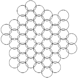
Figure 8: optimal spreading for $n=48$ nodes

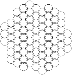
Figure 9: optimal spreading for $n=79$ nodes

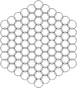
Figure 10: optimal spreading for n=91 nodes

VIII Conclusion

In this paper we have presented a distributed synchronous algorithm: MaxCover for maximum spreading without creating any coverage hole on an unbounded region. The movement of each sensor node only depends on its unique id and present position. No message exchange is required among the sensor nodes for execution of the algorithm. The number of rounds required for optimal spreading is $O(\sqrt{n})$.

Though in this paper we have assumed that all the sensor nodes are geometric points on a plane and initially all nodes are deployed at a point but same algorithm is also applicable for real (non-point) mobile sensors with following minor modifications of initial deployment. The nodes should be deployed in a place in such a way that they can form a completely connected graph with respect to their transmission range and they should have the knowledge of the position of the node with $id$ 0. It may be possible to have either prior knowledge of the location of node with $id$ 0 or after deployment the node with $id$ 0 informs its location to all other nodes by a broadcast. In each round, all unstable nodes move, either at the calculated location or any adjacent location of the calculated location. But during calculation of the next location, all unstable nodes should use calculated location of the previous round. All nodes which are allowed to be stable in any round should finally move to their calculated locations.

We have explained how proposed algorithm can be modified to achieve optimal energy consumption and how the algorithm can handle random deployment of sensor nodes. In future we will try to focus on the covering in presence of boundary and obstacles.

References

- [1] Fadi M. Al-Turjman, Hossam S. Hassanein, and Mohamed A. Ibnkahla. Connectivity optimization for wireless sensor networks applied to forest monitoring. In Proceedings of the 2009 IEEE international conference on Communications, ICC’09, pages 285–290, Piscataway, NJ, USA, 2009. IEEE Press.
- [2] Novella Bartolini, Tiziana Calamoneri, Emanuele G. Fusco, Annalisa Massini, and Simone Silvestri. Push & pull: autonomous deployment of mobile sensors for a complete coverage. Wireless Networks, 16(3):607–625, 2010.
- [3] Peter Brass. Bounds on coverage and target detection capabilities for models of networks of mobile sensors. ACM Trans. Sen. Netw., 3(2), June 2007.
- [4] Alex Brooks, Alexei Makarenko, Tobias Kaupp, Stefan B. Williams, and Hugh F. Durrant-Whyte. Implementation of an indoor active sensor network. In ISER, pages 397–406, 2004.
- [5] Mika Ishizuka and Masaki Aida. Performance study of node placement in sensor networks. In Proceedings of the 24th International Conference on Distributed Computing Systems Workshops - W7: EC (ICDCSW’04) - Volume 7, ICDCSW ’04, pages 598–603, Washington, DC, USA, 2004. IEEE Computer Society.
- [6] Lakshman Krishnamurthy, Robert Adler, Philip Buonadonna, Jasmeet Chhabra, Mick Flanigan, Nandakishore Kushalnagar, Lama Nachman, and Mark D. Yarvis. Design and deployment of industrial sensor networks: experiences from a semiconductor plant and the north sea. In SenSys, pages 64–75, 2005.
- [7] Jing Li, Ruchuan Wang, Haiping Huang, and Lijuan Sun. Voronoi-based coverage optimization for directional sensor networks. Wireless Sensor Network, 1(5):417–424, 2009.
- [8] Ming Ma and Yuanyuan Yang. Adaptive triangular deployment algorithm for unattended mobile sensor networks. IEEE Trans. Computers, 56(7), 2007.
- [9] Mana Saravi and Bahareh J. Farahani. Distance constrained deployment (DCD) algorithm in mobile sensor networks. In Proceedings of the 2009 Third International Conference on Next Generation Mobile Applications, Services and Technologies, NGMAST ’09, pages 435–440, Washington, USA, 2009. IEEE Computer Society.
- [10] Jian Tang, Bin Hao, and Arunabha Sen. Relay node placement in large scale wireless sensor networks. Computer Communications, 29(4):490–501, 2006.
- [11] Huanqi Tao and Heng Zhang. Forest monitoring application systems based on wireless sensor networks. In Proceedings of the 2009 Third International Symposium on Intelligent Information Technology Application Workshops, IITAW ’09, pages 227–230, Washington, DC, USA, 2009. IEEE Computer Society.
- [12] Bang Wang. Coverage problems in sensor networks: A survey. ACM Comput. Surv., 43(4):32, 2011.
- [13] Guiling Wang, Guohong Cao, and T. LaPorta. A bidding protocol for deploying mobile sensors. In Proceedings. 11th IEEE International Conference on Network Protocols (ICNP 2003), pages 315 – 324, Nov. 2003.
- [14] Guiling Wang, Guohong Cao, and Thomas F. LaPorta. Movement-assisted sensor deployment. IEEE Trans. Mob. Comput., 5(6):640–652, 2006.
- [15] Mohamed F. Younis and Kemal Akkaya. Strategies and techniques for node placement in wireless sensor networks: A survey. Ad Hoc Networks, 6(4):621–655, 2008.