Flux Transport Dynamo coupled with a Fast Tachocline Scenario

Abstract

The tachocline is important in the solar dynamo for the generation and the storage of the magnetic fields. A most plausible explanation for the confinement of the tachocline is given by the fast tachocline model in which the tachocline is confined by the anisotropic momentum transfer by the Maxwell stress of the dynamo generated magnetic fields. We employ a flux transport dynamo model coupled with the simple feedback formula of this fast tachocline model which basically relates the thickness of the tachocline to the Maxwell stress. We find that this nonlinear coupling not only produces a stable solar-like dynamo solution but also a significant latitudinal variation in the tachocline thickness which is in agreement with the observations.

1 Introduction

The tachocline is a thin layer (of radial extent $<20$ Mm) located at the base of the solar convection zone where the rotation changes from differential to the rigid rotation (e.g., Charbonneau et al. 1999). This layer is important in dynamo models for the generation and the storage of the toroidal fields. However the thinness of this layer made the confinement of the tachocline an intriguing problem. Spiegel & Zahn (1992) invoked strong anisotropic turbulent viscosity in the horizontal direction for the confinement of the tachocline. However several authors (e.g., Rudiger & Kitchatinov, 1997; Gough & McIntyre 1998) realized this purely hydrodynamical model to be inappropriate and proposed an alternative mechanism for the angular momentum transport. They have shown that a strongly anisotropic angular momentum transport is possible by invoking a weak fossil magnetic field in the radiative zone. This so-called slow tachocline model was later found to be questionable (e.g., Brun & Zahn, 2006; Strugarek, Brun & Zahn 2011, and references therein). Another plausible explanation for the confinement of the tachocline was that the Maxwell stress of the dynamo generated fields can provide a strong anisotropic angular momentum transport in the horizontal direction. For this mechanism to work, the dynamo-generated oscillatory magnetic field must penetrate the tachocline, which requires the value of the turbulent diffusivity to be $\geq 10^{9}$ cm²s^-1. This is known as the fast tachocline mechanism (Forgacs-Dajka & Petrovay 2001, 2002; Forgacs-Dajka 2003).

In the fast tachocline scenario, the thickness of the tachocline depends on the magnetic field in a nonlinear way. On the other hand, the thickness of the tachocline is an important input parameter of flux transport dynamo models. Therefore it is expected to affect the dynamo solution in an unexpected way. It is not even a priori clear whether the fast tachocline scenario and the flux transport dynamo model are compatible at all. The objective of the present work is to couple the simple feedback formula capturing the essential physics of the fast tachocline model in a flux transport dynamo model and to see its response. Details can be found in Karak & Petrovay (2013).

2 Formula relating the tachocline thickness and the magnetic fields

Following Forgács-Dajka & Petrovay (2001) the approximate relation between the mean (cycle averaged) tachocline thickness and Maxwell stress can be written as

$$d_{t}^{2}=\frac{C^{\prime}\eta_{t}}{\bar{B}_{p}(t)\bar{B}(t)}$$ (1)

where $\eta_{t}$ is the mean diffusivity in the tachocline, $\bar{B}$ and $\bar{B}_{p}$ ($=\sqrt{B_{r}^{2}+B_{\theta}^{2}}$) are the means value of the toroidal and the poloidal field in the tachocline defined in the following way.

$\bar{B}(t)=\frac{2}{\pi}\int_{0}^{\pi/2}\bar{B}(\theta,t)\,\mathrm{d}\theta$ and $\bar{B}_{p}(t)=\frac{2}{\pi}\int_{0}^{\pi/2}\bar{B}_{p}(\theta,t)\,\mathrm{d}\theta$
while $\bar{B}(\theta,t)$ and $\bar{B}_{p}(\theta,t)$ are the local radially averaged values of the toroidal and the poloidal field calculated as

$\bar{B}(\theta,t)=\frac{1}{2d_{0}}\int_{r_{t}-d_{0}}^{r_{t}+d_{0}}|B(r,\theta,t)|\,\mathrm{d}r$ with $d_{0}=0.015R$, and

$\bar{B}_{p}(\theta,t)=\frac{1}{2d_{0}}\int_{r_{t}-d_{0}}^{r_{t}+d_{0}}\bar{B}_{p}(r,\theta,t)\,\mathrm{d}r$ with $\bar{B}_{p}=\sqrt{(B_{r}^{2}+B_{\theta}^{2})}$

Note that the above relation (1) is strictly valid for the average (temporal and the latitudinal) values of $B_{p}$ and $B$, not for the actual values at a given point in space and time. However it is worthwhile to use the above simple physically motivated relation to explore its effect in the dynamo model.

3 Results

We use above relation for the tachocline thickness in a flux transport dynamo model (see Choudhuri 2011 for recent review). For the dynamo calculations we use the Surya code (Chatterjee, Nandy & Choudhuri 2004) with modified parameters presented in Karak & Petrovay (2013). Usually the flux transport dynamo model uses fixed value of the tachocline thickness. Here, however, we consider a variable tachocline thickness based on Eq. 1. The result for this calculation is shown in Figure 1. It is interesting to note is that this produces a stable solar-like dynamo solution. In addition, it produces a variable tachocline; the cyclic variation of tachocline thickness is somewhat larger (up to $\pm 30\%$) than the observational limit (e.g., Antia & Basu 2011).

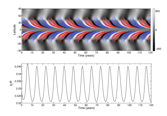
Figure 1: Upper panel: butterfly diagram of magnetic fields for variable tachocline thickness $d_{t}$ as given by Eq. (1). Contours show the butterfly diagram of the toroidal field in the tachocline. Blue contours correspond to positive toroidal field whereas red contours correspond to negative. The greyscale background shows the weak diffuse radial field on the solar surface. Lower panel: variation of tachocline thickness $d_{t}$ with time.

Next to explore the latitude dependence of tachocline thickness we write,

$$d_{t}^{2}=\frac{C^{\prime}\eta_{t}}{\bar{B}_{p}(\theta,t)\bar{B}(\theta,t)}.$$ (2)

Figure 2 shows the result. Note this procedure exibits a significant latitudinal variation in the tachocline thickness which agrees with the observations.

Figure 2: Same as Figure 1 but here the tachocline thickness [$d_{t}$] is determined by Eq. (2). In the lower panel, the dash-dotted, solid, dashed and dotted lines are the values of $d_{t}$ at $75^{0}$, $60^{0}$, $45^{0}$, and $15^{0}$ latitudes, respectively.

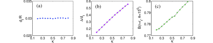
Figure 3: Variation of tachocline thickness [$d_{t}$] (a); of the amplitude variation of the tachocline thickness [$\Delta/d_{t}$] (b); and of toroidal field strength in the tachocline at $15^{\circ}$ latitude (c) as functions of $\kappa$ (the exponent in Eq. 3.

In order to explore the sensitivity of our quantitative results to details of the feedback formula, we generalize Eq. 2 in the following way,

$$d_{t}=\frac{(C^{\prime}\eta_{t})^{1/2}}{[\bar{B}_{p}(\theta,t)\bar{B}(\theta,t)]^{\kappa}}.$$ (3)

Recall that earlier we had $\kappa=0.5$. Although other values of $\kappa$ have no clear physical meaning, this offers a way to test the robustness of our results. We repeated our calculations with different values of $\kappa$ from $0.2$ to $0.8$. In every run, we set $C^{\prime}$ to fix the mean value of $d_{t}$ at around $0.03R$. Figure 3 shows the results. We see that the amplitude variation of $d_{t}$ increases with $\kappa$.

4 Conclusion

We coupled the simple feedback formula of the fast tachocline model, relating the Maxwell stress of the dynamo generated magnetic fields with the tachocline thickness, into a flux transport dynamo model which is successful in explaining many important aspects of the solar cycle (Choudhuri, Schüssler & Dikpati 1995; Dikpati & Charbonneau 1999; Choudhuri & Karak 2009; Karak 2011; Karak & Choudhuri 2011, 2012, 2013; Choudhuri & Karak 2012; Karak & Nandy 2012). We find that the dynamo model is robust against the nonlinearity introduced in this way. It produces a stable solar-like solution with a significant variation in the tachocline with latitude and time. The thickness of the tachocline varies from $0.02R$ to $0.1R$ as we move from low to high latitudes which is in agreement with the observations (e.g., Antia & Basu 2011). However the solar cycle variation of tachocline thickness is quite significant, and somewhat higher than what the observational constraints suggest.