Functional Renormalization Group Study of Phonon Mode Effects on Chiral Critical Point

Abstract

We apply the functional renormalization-group (FRG) equation to analyze the nature of the QCD critical point beyond the mean-field approximation by taking into consideration the fact that the soft mode associated with the QCD critical point is a linear combination of fluctuations of the chiral condensate and the quark-number density, rather than the pure chiral fluctuations. We first construct an extended quark-meson model in which a new field $\varphi$ corresponding to quark-number density is introduced to the conventional one composed of the chiral fields $(\sigma,\pi)$ and the quarks. The fluctuations of the quark-number density as well as the chiral condensate are taken into account by solving the FRG equation which contains $\sigma$ and $\varphi$ as coupled dynamical variables. It is found that the mixing of the two dynamical variables causes a kind of level repulsion between the curvature masses, which in turn leads to an expansion of the critical region of the QCD critical point, depending on the coupling constants in the model yet to be determined from microscopic theories or hopefully by experiments.

1 Introduction

The phase diagram of Quantum Chromodynamics (QCD) has been one of the main topics of theoretical high energy nuclear physics. In fact QCD phase diagram is expected to have a rich structure in a temperature ($T$) and quark-chemical potential ($\mu$) plane [1, 2, 3]. At low temperature and low chemical potential, the matter is considered to be strongly correlated and a naive perturbation does not work. Therefore non-perturbative methods are necessary to analyze the phase structure.

Lattice Monte-Carlo simulation is a first-principle and powerful approach for non-perturbative properties of QCD. At finite quark-chemical potential, however, we encounter the notorious sign problem which makes the statistical importance sampling method difficult. There are various proposals to overcome the sign problem [4], but the cold and dense region $\mu\gg T$ is still inaccessible by lattice simulations.

On the other hand, approaches based on effective models embodying proper symmetries with low-energy effective or collective degrees of freedom are legitimate and useful methods to investigate the phase diagram where we need to consider only low-lying soft modes with the energy scale of temperature $\sim 200$ MeV. Many investigations of the QCD phase diagram have been done on the basis of effective models, including (Polyalov loop extended-)Nambu-Jona-Lasinio ((P)NJL) model [5, 6, 7, 8, 9] or (Polyalov loop extended-) Quark-meson ((P)QM) model [11, 10, 12]. Whereas there is a strong model dependence of the position of the critical point [13], many chiral effective model calculations suggest the existence of a QCD critical point at finite temperature and quark-chemical potential where the crossover transition in the lower-$\mu$ region becomes a second order phase transition followed by a first-order in the higher-$\mu$ region.

In the vicinity of the QCD critical point, there is a critical region in which susceptibilities [14] or their higher derivatives [15] show critical behavior. In experimental searches of the QCD critical point, it is helpful to examine a shape and size of the critical region as discussed in Refs. [16, 17, 18, 19].

In general, there should exist at least one softening mode inherent in the second-order nature of the transition around a second order phase boundary. Analyses of the dynamical soft mode have been done on the basis of the quantum field theory [20, 21] and the Langevin equation [22]. Both analyses suggest that the soft mode around the critical point should be the quark-number density fluctuation or phonon mode (particle-hole excitation), in addition to the chiral order parameter. Since the quark number is a conserved quantity, its fluctuating mode ( phonon or sound mode) is necessarily a soft mode in the sense that its excitation energy $\omega$ vanishes in the small wave-number ($k$) limit as $\omega=c_{s}k$ where $c_{s}$ is the sound velocity. Then an effective potential as a function of the baryon-number density in addition to the chiral order parameter should be applied to investigate the critical phenomena accompanying the critical point [21, 22]. This situation is identical to the first-order liquid-gas phase transitions of water and the nuclear matter. As known in the $\sigma$-$\omega$ model [23, 24], the chiral order parameter couples with the baryon-number density mode at finite chemical potential. Consequently the linear combination of these two modes would be realized as the soft mode around the critical point. Although the inclusion of the quark-number density mode does not change the universality class, i.e., the critical point has the same universality class with the Ising model in three dimensions, it can change quantitative features, such as the size or shape of the critical region. It is worth emphasizing that they are of phenomenological importance, since an extension of the critical region toward higher-$T$ and lower-$\mu$ direction, which is found to be the case in the present work, implies that we may have more chance to probe the critical behavior by heavy-ion collision experiments.

Recently alternative possibilities of the phase structure are suggested, for example, inhomogeneous chiral condensation phases with the Lifshitz point [25, 26, 27] or multiple chiral critical points [28, 29, 30, 31, 32]. In the present work, however, we focus on the conventional phase structure with a single first-order phase boundary at low temperatures and a single critical point. Since the coupling between the quark-number density and the chiral condensate is inevitable at finite chemical potential, the analysis in the present work is also appropriate for the other candidates of the phase structure.

Near the second-order phase boundary, fluctuations of the soft mode are enhanced and the mean-field approximation breaks down. We need to include the soft mode and its fluctuation effects in order to correctly describe the QCD critical point and its critical region. The functional renormalization group (FRG) method [34, 33, 35] is one of the machineries to evaluate an effective action beyond the mean-field approximation, see [36, 37] for a general introduction. Although there are many analyses on the QCD phase diagram using FRG [38, 16, 39, 40, 41, 42, 43] where effective models are mostly used, there have been only few works on the QCD critical point which include the quark-number density fluctuation as well as chiral modes beyond the mean-field approximation.

In the present work, we start from an effective model including the quark-number density fluctuation as well as the sigma and pion modes. We apply the FRG method to take into account the fluctuations of the soft mode. A key quantity in our analysis is a strength of the coupling between the sigma and quark-number density. We thereby examine not only the phase structure around the critical point but also the sensitivity of the critical region to the sigma-density coupling strength.

This paper is organized as follows. In Sec. 2, an evolution equation for the scale dependent effective potential is derived. In Sec. 2.1, we introduce an effective model which should describe the dynamics near the QCD critical point. The new field $\varphi$ is introduced in order to describe the quark-number density. The FRG method and a suitable approximation for our model is discussed in Sec. 2.2. Results of numerical calculations are given in Sec. 3. Section 4 is devoted to the summary and outlook.

2 Formulation

2.1 Effective model near QCD critical point

In this section we introduce an effective model for describing the two-flavor QCD near the critical point. Our starting point is the quark-meson (QM) model [10] which is one of the chiral effective models of the low-energy QCD. Since the QM model explicitly contains the meson degrees of freedom in the Lagrangian, we can easily incorporate the fluctuations of the mesonic modes in the framework of the FRG. The Lagrangian of the QM model for 2-flavor and 3-color degrees of freedom reads

$$\begin{split}{L}_{\rm QM}&=\bar{\psi}[i{\ooalign{\hfil/\hfil\crcr$\partial$}}-g_{s}(\sigma+i\gamma_{5}\vec{\tau}\cdot\vec{\pi})]\psi+\frac{1}{2}(\partial_{\mu}\sigma)^{2}+\frac{1}{2}(\partial_{\mu}\vec{\pi})^{2}-U(\sigma^{2}+\vec{\pi}^{2})+c\sigma,\end{split}$$ (1)

with the mesonic potential $U(\sigma^{2}+\vec{\pi}^{2})=\frac{m^{2}}{2}(\sigma^{2}+\vec{\pi}^{2})+\frac{\lambda}{4!}(\sigma^{2}+\vec{\pi}^{2})^{2}$. The explicit symmetry breaking term ($c\sigma$) corresponds to a finite current quark mass. Except the explicit symmetry-breaking term, the Lagrangian is invariant under the chiral $SU(2)_{L}\times SU(2)_{R}$ transformation.

The QM model has been extensively used as the starting model for the FRG analysis of the global structure of the QCD phase diagram [11, 10, 12], i.e., a chiral symmetry breaking at low temperature and low chemical potential and its restoration at high temperature and/or high chemical potential. Many previous works using the QM model rely on the analysis of the effective potential as a function of the chiral order parameter ($\sigma$) : Notice that the $\sigma$ field in Eq. (1) couples to the quark scalar density $\bar{\psi}\psi$, the expectation value of which is the primary chiral order parameter. In those analyses, the finite quark density effects are taken into account through the chemical potential dependence of the effective potential. As a result, the critical behaviors associated with the QCD critical point were caused only by the fluctuation of the chiral order parameter or scalar density. The soft mode associate with the QCD critical point is, however, a linear combination of the chiral order parameter and the quark-number density [20, 21, 22], which has not been properly taken into account in the previous works based on the FRG analysis despite of its importance. Thus an FRG analysis using the effective potential as a function of not only the chiral order parameter but also the quark-number density as an independent additional degree of freedom is of imperative importance to understand the phase structure near the critical point precisely.

In this work in order to effectively incorporate the fluctuation of the quark-number density, we extend the QM model. We introduce a new bosonic degree of freedom $\varphi$ following the analyses in Refs. [21] and [22]: the new field $\varphi$ corresponds to the quark-number density with an appropriate normalization and naturally couples to $\bar{\psi}\gamma_{0}\psi$. Thus our effective model takes the following form:

$$\begin{split}L&=\bar{\psi}[i{\ooalign{\hfil/\hfil\crcr$\partial$}}-g_{s}(\sigma+i\gamma_{5}\vec{\tau}\cdot\vec{\pi})+g_{d}\varphi\gamma_{0}]\psi+\frac{1}{2}(\partial_{\mu}\sigma)^{2}+\frac{1}{2}(\partial_{\mu}\vec{\pi})^{2}+\frac{1}{2}(\partial_{\mu}{\varphi})^{2}\\ &-U(\sigma^{2}+\vec{\pi}^{2})-\frac{m_{\varphi}^{2}}{2}\varphi^{2}+c\sigma.\end{split}$$ (2)

Whereas the effective model (2) looks similar to the NJL model with a vector interaction [44, 28, 45, 46, 48, 47], our model has only the mode corresponding to the zeroth component of the vector fields. One might suspect that the other components of the vector fields should be included in order to respect the manifest Lorentz invariance. It should be, however, noted that we apply the model to finite chemical potential where baryonic matter is formed and the Lorentz symmetry is explicitly broken. Moreover the other components of the vector fields are irrelevant to the critical phenomena near the QCD critical point because we do not have finite condensations of the spatial components and then the spatial components is decoupled from the chiral modes. In this sense, our model embodies enough ingredients for the investigation of the critical phenomena associate with the QCD critical point.

There also exists a difference in the nature between the $\varphi$ and the zeroth component of the vector fields. In our set up, the field $\varphi$ which is supposed to describe a particle-hole excitation and causes an attractive interaction between two quarks [49] while the zeroth component of the vector field is usually introduced as a source of repulsive interaction. We will come to this point later.

At finite chemical potential, both the chiral condensate and quark-number density take finite expectation values, $\langle\sigma\rangle\neq 0$ and $\langle\varphi\rangle\neq 0$. We calculate the effective potential with the fluctuations of the chiral modes and $\varphi$ by solving the FRG equation and determine the expectation values of these modes from the minimum of the effective potential.

2.2 Functional renormalization group

In order to evaluate the effective potential with the fluctuations of the quark-number density as well as the chiral modes, we adopt the FRG equation. We make an approximation suited to solve the QM model and derive an evolution equation for a scale dependent effective potential.

In the FRG approach, we introduce a scale ($k$) dependent effective action $\Gamma_{k}$ which should satisfy the following properties at ultraviolet ($k=\Lambda$) and infrared ($k=0$) scale:

$$\begin{split}\Gamma_{\Lambda}&=S\\ \Gamma_{0}&=\Gamma\;,\end{split}$$ (3)

where $S$ and $\Gamma$ are the classical action and quantum effective action, respectively.

We can construct the scale dependent effective action by inserting a mass-like term into the Lagrangian which controls the quantum and thermal contribution to the effective action. For the bosonic modes, we insert the bosonic mass-like term $R_{kB}(p)\phi(p)\phi(-p)$ into the Lagrangian where $R_{kB}(p)$ is an arbitrary function satisfying the following condition:

$$\begin{split}R_{kB}(p)\sim k^{2}\;\;{\rm for}\;\;p^{2}\ll k^{2},\\ R_{kB}(p)\sim 0\;\;{\rm for}\;\;p^{2}\gg k^{2}.\\ \end{split}$$ (4)

At the infrared scale ($k=0$), $R_{k}$ is zero for any momentum, and $\Gamma_{k}$ becomes the quantum effective action. At the ultraviolet scale ($k=\Lambda$), all modes acquire large masses, $m^{2}\to m^{2}+\alpha\Lambda^{2}$ where $\alpha$ is a proportional coefficient in $R_{k}(p)$, $R_{\Lambda}(p)\simeq\alpha\Lambda^{2}$. As a result, $R_{k}$ prevents the propagation of all the fluctuation, and $\Gamma_{\Lambda}$ becomes the classical action. Thus one finds that the conditions for the $\Gamma_{k}$ are satisfied. At an intermediate scale, $R_{k}(p)$ suppresses propagation of the modes whose momentum are smaller than $k$. Thus we can interpret the $\Gamma_{k}$ as an effective action which contains the fluctuations whose momentum scales are larger than $k$. The above procedure can be extended to the fermionic modes by introducing the mass-like term $\bar{\psi}(p)R_{kF}(p)\psi(p)$ where $R_{kF}$ has Dirac indices. (See, e.g., Ref. [36]).

In the present work, we choose the so-called optimized cutoff function [50] whose form is

$$\begin{split}R_{k\rm B}(p)&=(k^{2}-\vec{p}\;^{2})\theta(k^{2}-\vec{p}\;^{2})\;\;\;{\rm for\;Bosons}\\ R_{k\rm F}(p)&={\ooalign{\hfil/\hfil\crcr$\vec{p}$}}\left(\sqrt{\frac{k^{2}}{\vec{p}\;^{2}}}-1\right)\theta(k^{2}-\vec{p}\;^{2})\;\;\;{\rm for\;Fermions}\;.\end{split}$$ (5)

The evolution of the $\Gamma_{k}$ with scale $k$ is described by the FRG equation [35]:

$$\begin{split}k\frac{\partial\Gamma_{k}}{\partial k}&=-{\rm Tr}\left[\frac{\partial_{k}R_{k\rm F}}{R_{k\rm F}+\Gamma_{k}^{(2,0)}}\right]_{\rm F}+\frac{1}{2}{\rm Tr}\left[\frac{\partial_{k}R_{k\rm B}}{R_{k\rm B}+\Gamma_{k}^{(0,2)}}\right]_{\rm B}\;,\end{split}$$ (6)

where the trace runs over Dirac, color and flavor indices as well as momentum. The superscript ${(a,b)}$ in $\Gamma_{k}^{(a,b)}$ denotes $a(b)$ times fermionic (bosonic) functional derivative of the $\Gamma_{k}$. The first and second terms of r.h.s of (6) are the fermionic and bosonic contributions respectively.

To solve the FRG equation of the scale dependent effective action (6), we need scale ($k$) dependencies of the 2-point functions $\Gamma_{k}^{(2,0)}$ and $\Gamma^{(0,2)}_{k}$. In general, the FRG equation for the $n$-point function depends on up to the $(n+2)$-point function and the set of the FRG equations for $n$-point functions forms an infinite tower of the equations. In practice, we introduce some approximations in order to close the tower of equations up to finite $n$-point functions. In the present work, we apply the so-called local potential approximation (LPA) to the effective action. We assume the form of the scale dependent effective action as

$$\begin{split}\Gamma_{k}^{LPA}&=\bar{\psi}[i{\ooalign{\hfil/\hfil\crcr$\partial$}}-g_{s}(\sigma+i\gamma_{5}\vec{\tau}\cdot\vec{\pi})-g_{d}\varphi\gamma_{0}+\mu\gamma_{0}]\psi+\frac{1}{2}(\partial_{\mu}\sigma)^{2}+\frac{1}{2}(\partial_{\mu}\vec{\pi})^{2}+\frac{1}{2}(\partial_{\mu}{\varphi})^{2}\\ &-U_{k}(\sigma^{2}+\pi_{0}^{2},\varphi)-c\sigma\;,\end{split}$$ (7)

where $U_{k}$ is a scale dependent effective potential such that it agrees with a usual effective potential at $k=0$. Except for the small explicit breaking term $c\sigma$, which can be treated as a perturbation for the symmetric effective action, the Lagrangian (2) respects the chiral symmetry. To a good approximation, we can regard $U_{k}$ as a function of $\sigma^{2}+\vec{\pi}^{2}$ and $\varphi$.

Here we neglect the scale dependence of the wave function renormalization for simplicity. It would be important for the discussion of the possibility of the inhomogeneous condensation phase but it is out of the scope of this work.

We also neglect the evolutions of the Yukawa coupling $g_{s}$ and the density coupling $g_{d}$. The inclusion of the scale dependencies of these couplings might change the global structure of the phase diagram such as the position of the QCD critical point or the slope of the first-order phase boundary of the chiral phase transition. Near the QCD critical point, however, the contributions from the light bosons are enhanced and the scale dependence of $g_{s}$ and $g_{d}$ would not change the local phase structure, i.e., the shape or size of the critical region. Thus the scale dependence could be neglected when the critical region is only concerned.

Now the 2-point functions in the r.h.s of (6) is given by the functional derivatives of the LPA effective action:

$$\begin{split}\Gamma^{(2,0)}_{k}&\rightarrow\frac{\partial^{2}\Gamma_{k}^{LPA}}{\partial\bar{\psi}\partial\psi}\\ \Gamma^{(0,2)}_{k\;a,b}&\rightarrow\frac{\partial^{2}\Gamma_{k}^{LPA}}{\partial\phi_{a}\partial\phi_{b}}\;.\end{split}$$ (8)

Using LPA, we can obtain an evolution equation for the scale dependent effective potential. Substituting the LPA ansatz (7), (8) and the optimized cutoff function (5) into (6), we obtain the flow equation for the effective potential:

$$\begin{split}\frac{\partial U_{k}}{\partial k}&=\frac{k^{4}}{12\pi^{2}}\Bigg{[}-2N_{f}N_{c}\left[\frac{1}{E_{q}}\tanh\left(\frac{E_{q}+(\mu+g_{d}\varphi)}{2T}\right)+\frac{1}{E_{q}}\tanh\left(\frac{E_{q}-(\mu+g_{d}\varphi)}{2T}\right)\right]\\ &\;\;\;\;\;\;\;\;\;\;\;\;\;\;\;\;+\sum_{i=\pm}\frac{1}{E_{i}}\coth\left(\frac{E_{i}}{2T}\right)+\frac{3}{E_{\pi}}\coth\left(\frac{E_{\pi}}{2T}\right)\Bigg{]},\\ \end{split}$$ (9)

where the scale dependent particle energies $E_{\alpha}$ ($\alpha=q$, $\pi$ and $\pm$) are defined as

$$\begin{split}E_{\alpha}^{2}&=k^{2}+M_{\alpha}^{2},\\ M_{q}^{2}&=g^{2}\sigma^{2},\;M_{\pi}^{2}=\frac{U^{\prime}}{\sigma},\\ M_{i=\pm}^{2}&=\frac{U^{\prime\prime}+\ddot{U}\pm\sqrt{(U^{\prime\prime}-\ddot{U})^{2}+4\dot{U}^{{}^{\prime}2}}}{2}.\end{split}$$ (10)

Here we have used the following notation

$$U^{\prime}=\frac{\partial U}{\partial\sigma},\;\;\dot{U}=\frac{\partial U}{\partial\varphi}\;.$$ (11)

$M_{\pi}^{2}$ and $M_{i}^{2}$ are understood as the squared curvature masses of the $\pi$ and the linear combination of $\sigma$ and $\varphi$.

Since the scale dependent effective action at the UV scale agrees with the classical action (3), the initial condition of the flow equation (LABEL:eq:LPA_flow_equation) reads

$$\begin{split}U_{\Lambda}(\sigma^{2}+\vec{\pi}^{2},\varphi)=a(\sigma^{2}+\vec{\pi}^{2})+b(\sigma^{2}+\vec{\pi}^{2})^{2}+\frac{M^{2}_{\varphi}}{2}\varphi^{2}\;.\end{split}$$ (12)

By solving the flow equation from $k=\Lambda$ to $k=0$, we obtain the effective potential with the fluctuation effects incorporated. The expectation values of the $\sigma$ and $\varphi$ are determined by minimizing the effective potential at $k=0$:

$$\begin{split}\frac{\partial U}{\partial\sigma}\Bigg{|}_{\sigma_{0},\varphi_{0}}-c=\frac{\partial U}{\partial\varphi}\Bigg{|}_{\sigma_{0},\varphi_{0}}=0\;.\end{split}$$ (13)

We obtain the effective potential at various temperatures and chemical potentials, and the phase structure is determined by the chiral order parameter behavior.

3 Numerical results

In this section, we show numerical results. One of our concerns is the sensitivity of the phase structure to the strength of the mixing between the chiral condensate and the quark-number density, i.e., the magnitude of the density coupling $g_{d}$.

First we calculate the phase diagrams with $g_{d}$ being varied. We show the position of the QCD critical point slightly moves to a higher temperature direction with increasing $g_{d}$.

Next we describe the critical region which is associated with the QCD critical point. Finally we calculate the curvatures of the effective potential. We show that a kind of level repulsion between the curvature masses occurs around the QCD critical point at finite $g_{d}$. This level repulsion causes an expansion of the critical region.

3.1 Calculation method and parameter fixing

We solve the flow equation (LABEL:eq:LPA_flow_equation) numerically on a grid in the field space. Since both $\sigma$ and $\varphi$ can take non-vanishing expectation values, we have to prepare the $U_{k}$ values on the two-dimensional grid of discrete field values in the $\sigma$ and $\varphi$ space. Derivatives of the effective potential used in the numerical calculation are given by finite differences. This reduces the flow equation to a coupled ordinary differential equations which can be integrated out with a standard method. We solve it by using the fourth-order Runge-Kutta method.

There are few works using a 2-dimensional grid method for dynamical fields and, only very recently, it has been developed by several researchers including one of the present authors on the studies of QCD phase diagram with isospin chemical potential [51, 52] as well as the phase diagram of 2-color QCD [53]. In comparison with the Taylor method in which the effective potential is locally evaluated around a scale dependent minimum, the grid method captures the global structure of the effective potential in the field space and is well suited to investigate the critical region with which the first order phase boundary is connected.

$a/{\Lambda^{2}}$	$b$	${c}/{\Lambda^{3}}$	$M_{\varphi}^{2}/\Lambda^{2}$	$\Lambda$ MeV	$g_{s}$
0.3224	0.25	0.0045	0.1	900	3.2

Table 1: Table of the initial parameters for the numerical calculations

In the present calculation, we choose the ultraviolet scale as $\Lambda=900$MeV. Our effective model has six parameters $a,b,c,g_{s},M_{\varphi}$ and $g_{d}$. The first four parameters have been determined to reproduce the vacuum physical values such as the pion mass, sigma mass, pion decay constant and constituent quark mass [52].

We can not, however, determine the remaining two parameters $M_{\varphi}$ and $g_{d}$ because at present any experimental data for the collective excitation corresponding to the particle-hole mode (phonon mode) in quark matter is not available. In principle we could determine these parameters from microscopic theories such as QCD itself or the NJL model. However the main purpose of this work is to examine the sensitivity of the critical region to the mixing between the $\sigma$ and $\varphi$ then we treat $M_{\varphi}$ and $g_{d}$ as free parameters and examine responses to their variation. Here we fix $M^{2}_{\varphi}=0.1\Lambda^{2}$ and change $g_{d}$. The phase structure is determined by the relative strength $g_{v}/M^{2}_{\varphi}$. For example, the ordinary results of the QM model are reproduced by taking $g_{v}/M^{2}_{\varphi}\rightarrow 0$. Our choice of the parameter set is summarized in Table 1.

3.2 Phase structure

Before studying the critical region, we start with an analysis of the phase structure with varying $g_{d}$.

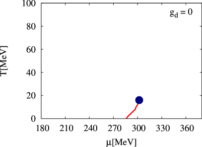
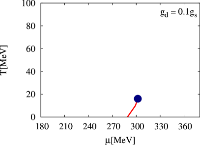
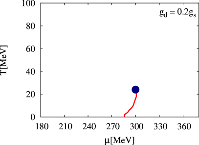
Figure 1: Phase diagram for four different $g_{d}$ ($0$, $0.1g_{s}$, $0.2g_{s}$ and $0.3g_{s}$). The solid line denotes the first-order phase boundary while the blue closed circle represents the critical point. A green line and black circle in $g_{d}=0.3g_{s}$ denote second first-order phase boundary and its critical end point.

In Fig. 1, the phase diagrams are shown for four fixed values of $g_{d}$. In the present work, we have generalized the previous results in the zero density-coupling case [52] to the finite couplings. We find the QCD critical point for each $g_{d}$ value. The locations of the QCD critical point are, in unit of MeV, at ($T_{cp}$,$\mu_{cp}$) $\simeq$ $(15,303),(16,303),(28,300)$ and $(42,284)$ for $g_{d}=0,0.1g_{s},0.2g_{s}$ and $0.3g_{s}$, respectively. For the temperature below the critical point, we find the first-order phase boundary which separates a chiral restored phase (higher $\mu$) and a broken phase (lower $\mu$). At the critical point, the phase transition is second order. Beyond the critical point, the phase transition becomes crossover and the pseudo critical line is not shown in the phase diagram.

The position of the critical point slightly rises to a higher temperature direction with increasing $g_{d}$. This is an opposite behavior to the well known results in the NJL model with the vector interaction [28, 45, 46, 47]. This is because our effective model corresponds to the attractive vector interaction case ($G_{V}<0$). In fact, a similar behavior is found in the mean field approximation of the NJL model with an artificial attractive vector interaction [48].

In the figure for $g_{d}=0.3g_{s}$, one sees another critical point at ($T_{cp}$,$\mu_{cp}$) $\simeq$ (80,351) MeV from which another first-order phase boundary is extended to the lower-$T$ direction. This should be an artifact of our model. This additional critical point and its associated first-order phase boundary appear only with large couplings such as $g_{d}=0.3g_{s}$ and they belong to a different branch from the QCD critical point. The magnitude of the chiral condensate is sufficiently smaller than the vacuum expectation value and jumps from about 10 MeV to a few MeV across the first-order phase boundary. At $g_{d}=0.3g_{s}$, the attractive force between two quarks is too strong and causes another stable minimum of the effective potential in the high density and small chiral condensation region.

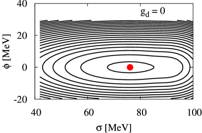
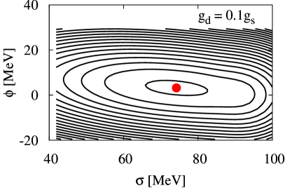
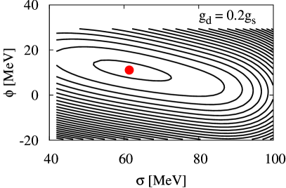
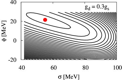
Figure 2: Contours of the effective potential in the $\sigma$ and $\varphi$ space near the critical point for varying $g_{d}$. The solid points show the minimum of the effective potential.

In Fig. 2, the effective potential contour is shown for several $g_{d}$ values at temperature and chemical potential close to the critical point. Since the phase transition is second order at the QCD critical point, there is a flat direction on the effective potential around the minimum.

For $g_{d}=0$, $\varphi$ is decoupled from the chiral modes then the mixing term such as $\sigma^{2}\varphi$ does not arise in the effective potential. As a result, we can see the flat direction is parallel to the $\sigma$ axis.

On the other hand, for $g_{d}\neq 0$, there is a mixing between $\sigma$ and $\varphi$ and the expectation value of $\varphi$ is not zero.

The flat direction is tilted to the direction of the linear combination of $\sigma$ and $\varphi$ directions and the $\sigma$ direction is no longer special. These behaviors are also found in a calculation on the NJL model [21]. The angle between the flat direction and the $\sigma$ direction becomes larger with increasing $g_{d}$ as the mixing between the $\sigma$ and $\varphi$ becomes stronger.

The singular behavior of susceptibilities shown in the next section is mediated by the fluctuation along the flat direction of the effective potential. For finite $g_{d}$, the flat direction is the linear combination of the $\sigma$ and $\varphi$ directions and the critical behaviors are attributed to the fluctuation of the linear combination. On the other hand, in the case of $g_{d}=0$ (the QM model), the flat direction is parallel to the $\sigma$ axis and the critical behaviors are attribute to only the fluctuation of the chiral order parameter.

3.3 Susceptibility

The information on the size of the critical region is important for experiments in search of the QCD critical point. We define the critical region by using the quark-number susceptibility $\chi_{q}$ given as the response of the quark-number density $n_{q}$ to $\mu$:

$$\chi_{q}\equiv\frac{\partial n_{q}}{\partial\mu}=\frac{\partial^{2}P(T,\mu)}{\partial\mu^{2}}\;,p$$ (14)

where the pressure $P$ is given by $P(T,\mu)=-U(\sigma_{0},\phi_{0})$. For the comparison of the shape and size of the critical region for different $g_{d}$, it is convenient to use a normalized susceptibility $\chi_{q}^{\rm{n}}$, i.e., the ratio to that of the mass-less free quark gas $\chi_{q}^{\rm free}$:

$$\begin{split}\chi_{q}^{\rm free}&\equiv\frac{2N_{c}N_{f}}{6}\left[T^{2}+\frac{3\mu^{2}}{\pi^{2}}\right]\\ \chi_{q}^{\rm{n}}&\equiv\chi_{q}/\chi_{q}^{\rm free}\;.\\ \end{split}$$ (15)

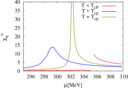
Figure 3: Plots of the normalized quark-number susceptibility $\chi_{q}^{\rm{n}}=\chi_{q}/\chi_{q}^{\rm free}$ with chemical potential at $g_{d}=0.2g_{s}$. The red/blue line represent the $\chi_{q}^{\rm{n}}$ at T below/beyond the $T_{cp}$. The green line is at $T=T_{cp}$.

In Fig. 3, $\chi_{q}^{\rm{n}}$ at $g_{d}=0.2g_{s}$ is shown as a function of quark-chemical potential for three different temperatures. For temperatures below the critical temperature $T_{cp}$, there is a discontinuity in $\chi_{q}^{\rm{n}}$ at the first-order phase boundary. For temperatures above $T_{cp}$, $\chi_{q}^{\rm{n}}$ is continuous as a function of $\mu$ and has a peak at the crossover phase boundary. The peak height becomes higher with $T$ approaching to $T_{cp}$. At $T=T_{cp}$, the peak height of $\chi_{q}^{\rm{n}}$ diverges. Near the QCD critical point, we find the same behavior of the $\chi_{q}^{\rm{n}}$ for all $g_{d}$.

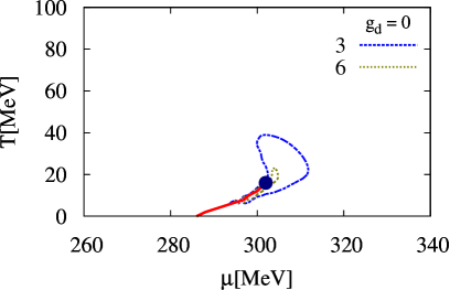
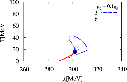
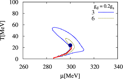
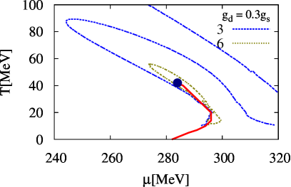
Figure 4: Contours of the normalized quark-number susceptibility $\chi_{q}^{\rm{n}}=\chi_{q}/\chi_{q}^{\rm free}$ around the critical point for $\chi_{q}^{\rm{n}}=3$ and $6$. The red line denote the first-order phase boundary. The blue solid circle represent the QCD critical point.

In Fig. 4, the contour plots of $\chi_{q}^{\rm{n}}$ with two fixed values, $\chi_{q}^{\rm{n}}=3,6$, are shown for varying $g_{d}$. The criticality near the QCD critical point is characterized by the enhancement of $\chi_{q}$. In the following, we define the critical region by $\chi_{q}^{\rm{n}}>3$.

For $g_{d}=0$, we have the critical region which has 10 MeV extent both in the $T$ and $\mu$ directions. The size of the critical region for $g_{d}=0$ is consistent with the previous work [16] and the width of the critical region is shrunken in the $\mu$ direction by almost one order of magnitude compared with the mean-field calculation [16].

For finite $g_{d}$, the critical region is deformed from that at $g_{d}=0$. We observe the expansion of the critical region to the crossover phase transition direction with increasing $g_{d}$. The shape and size of the critical region are quite sensitive to $g_{d}$ such that it shows drastic deformation while the position of the QCD critical point moves only slightly. At $g_{d}=0.3g_{s}$, the critical region is elongated to the cross over side twice as large as that for $g_{d}=0$.

This expansion can be partly understood by looking at the curvature masses of the linear combination of the $\sigma$ and $\varphi$, as demonstrated in the following.

3.4 curvature masses

In order to give the understanding of the expanding behavior of the critical region, we calculate the curvature masses of the linear combination of the $\sigma$ and $\varphi$. The masses $M_{+}$ and $M_{-}$ are defined as a bigger and smaller eigenvalue of the curvature matrix, respectively:

$$M=\begin{pmatrix}\frac{\partial^{2}U}{\partial\sigma\partial\sigma}&\frac{\partial^{2}U}{\partial\sigma\partial\varphi}\\ \frac{\partial^{2}U}{\partial\varphi\partial\sigma}&\frac{\partial^{2}U}{\partial\varphi\partial\varphi}\end{pmatrix}\Bigg{|}_{\sigma_{0},\varphi_{0}}\;.$$ (16)

In Fig. 5, the curvature masses $M_{\pm}$ at $T=T_{cp}$ are shown as functions of quark-chemical potential for $g_{d}=0$ (left) and $g_{d}=0.2g_{s}$ (right).

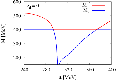
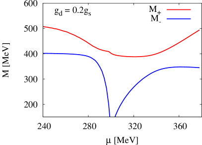
Figure 5: Plots of the curvature masses $M_{\pm}$ near the critical point with chemical potential. The left and right panel are at $g_{d}=0$ and $g_{d}=0.2g_{s}$ respectively.

At $g_{d}=0$, there is no mixing between the $\sigma$ and $\varphi$ then the non-diagonal parts of the mass matrix (16) are always zero, and thus we can identify the $\sigma$ and $\varphi$ modes individually. Since the $\varphi$ is decoupled from the matter sector, the curvature mass of the $\varphi$ is constant ($\sim 400$ MeV) with chemical potential varied while the sigma mass decreases below the mass of the $\varphi$ and vanishes at the critical point. Beyond the critical point, the $\sigma$ mass increases monotonically.

In contrast, the non-diagonal parts of the mass matrix (16) do not vanish for $g_{d}\neq 0$ so that the $\sigma$ and $\varphi$ are mixed. At $g_{d}=0.2g_{s}$, $M_{-}$ stays constant ($\sim 400$ MeV) while $M_{+}$ decreases below the critical chemical potential. When $M_{+}$ gets close to $M_{-}$, $M_{-}$ starts to decrease and vanishes at the critical point. We observe a kind of level repulsion near the critical point between $M_{+}$ and $M_{-}$ which is familiar in a perturbation theory in quantum mechanics [54]. Beyond the critical point, $M_{-}$ increases until 340 MeV and becomes almost constant. $M_{+}$ increases again while $M_{-}$ increases and approaches a constant value. We found these behaviors of the $M_{+}$ and $M_{-}$ generally for $g_{d}\neq 0$.

Note that the softening behavior shown here does not correspond to the dynamical softening of these modes. In order to see the dynamical softening of the modes, one has to calculate spectral functions of the $\sigma$ or $\varphi$ modes in which one would find a dissipative zero mode in the space-like region of the spectral function [20, 21, 22, 55].

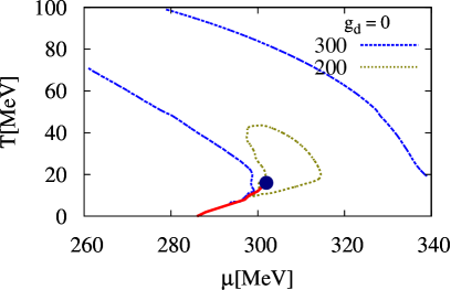
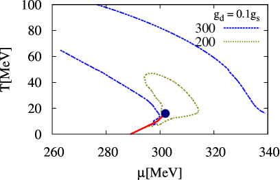
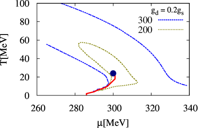
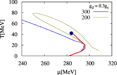
Figure 6: Contours of the smaller curvature mass $M_{-}$ for varying $g_{d}$. The contours are shown for $M_{-}=200$ and $300$ MeV. The red lines denote the first-order phase boundary. The blue solid circles represent the QCD critical point.

In Fig 6, we show a contour map for $M_{-}$ with varying $g_{d}$. For each $g_{d}$, $M_{-}$ is close to zero in the vicinity of the critical point. The softening of the linear combination of the $\sigma$ and $\varphi$ causes the critical behavior on the susceptibility.

In the following, we call the area in which $M_{-}<200$ MeV the softening region. For each $g_{d}$, we can see the softening region almost coincide with the critical region, i.e., the region in which $\chi_{q}^{\rm{n}}>3$ in Fig. 4. The softening region is also expanded to the crossover phase transition direction with $g_{d}$ being increased.

The level repulsion of the curvature masses precisely corresponds to the expanding behavior of the critical region. The curvature mass $M_{-}$ is reduced when the density coupling or the non-diagonal parts of the mass matrix (16) is finite. The non-diagonal parts of (16) become larger as $g_{d}$ increases. As a result, the level repulsion between $M_{+}$ and $M_{-}$ becomes larger and the region with small $M_{-}$ also gets expanded. It simply follows that the inclusion of the mixing between the $\sigma$ and $\varphi$ and does not depend on the details of interactions, for example, repulsive or attractive force.

4 Summary

We have examined the influence of the mixing between the chiral condensation and the quark-number density on the critical region around the QCD critical point. The fluctuations of the quark-number density as well as the chiral modes were taken into account through the functional renormalization group (FRG) equation.

We have extended the quark meson model to a new effective model which is appropriate for the correct description of the dynamics near the QCD critical point. In addition to the quarks and chiral modes ($\sigma$ and $\vec{\pi}$), the new effective model contains a new field $\varphi$ which corresponds to the quark-number density. The magnitude of the mixing between the $\sigma$ and $\varphi$ was determined by a density couping $g_{d}$.

We derived the flow equation for the scale dependent effective action with the fluctuation of the density field at a finite temperature and quark-chemical potential. The flow equation for the scale dependent effective potential was solved numerically on a two-dimensional grid of the chiral condensate ($\sigma$) and quark-number density ($\varphi$).

We found that the QCD critical point exists for varying $g_{d}$ while its position slightly moves to the higher temperature and lower quark-chemical potential direction as $g_{d}$ increases. The quark-number susceptibility was enhanced around the critical point.

In contrast, we have shown the shape and size of the critical region was quite sensitive to the magnitude of the mixing term. We have shown that the critical region is enlarged to a lower chemical potential and higher temperature direction when we increase the density coupling $g_{d}$.

In order to confirm the expanding behavior, we also calculated the curvature masses of the linear combination of the $\sigma$ and $\varphi$. It turned out that the critical region was almost identical to the softening region where the curvature of the effective potential becomes small. The softening of the linear combination of the $\sigma$ and $\varphi$ causes the critical behavior.

We have shown that the origin the expanding behavior of the critical region and the softening region level repulsion of the curvature masses given by the linear combination of the chiral condensate and the quark-number density. The large level repulsion at large $g_{d}$ makes the critical and softening region wider. The level repulsion is a generic consequence of the mixing between the chiral condensate and the quark-number density.

As a future work, it is interesting to investigate higher moments of the quark-number density or the charge-number density including the quark-density coupling and the fluctuation of the quark-number density. The higher moments are considered to show the stronger criticality [15] and would be more sensitive to the mixing than the quark-number susceptibility. In the present work, we have considered the simplest case of the coupling and treated its strength as a free parameter but it should be determined by a more microscopic model or experiments. The exact determinations of the strength or detailed form of the mixing also awaits future studies.

References

- [1] P. Braun-Munzinger and J. Wambach, Rev. Mod. Phys. 81, 1031 (2009).
- [2] B. Friman, C. Hohne, J. Knoll, S. Leupold, J. Randrup, R. Rapp and P. Senger, Lect. Notes Phys. 814, 1 (2011).
- [3] K. Fukushima and T. Hatsuda, Rept. Prog. Phys. 74, 014001 (2011).
- [4] Ph. de Forcrand, PoS LAT2009, 010 (2009).
- [5] M. Asakawa and K. Yazaki, Nucl. Phys. A 504, 668 (1989).
- [6] T. Hatsuda and T. Kunihiro, Phys. Rept. 247, 221 (1994) [hep-ph/9401310].
- [7] M. Buballa, Phys. Rept. 407, 205 (2005).
- [8] K. Fukushima, Phys. Lett. B 591, 277 (2004).
- [9] C. Ratti, M. A. Thaler and W. Weise, Phys. Rev. D 73, 014019 (2006).
- [10] D. U. Jungnickel and C. Wetterich, Phys. Rev. D 53, 5142 (1996) [hep-ph/9505267].
- [11] J. Braun, H.-J. Pirner and K. Schwenzer, Phys. Rev. D 70, 085016 (2004).
- [12] B.-J. Schaefer, J. M. Pawlowski and J. Wambach, Phys. Rev. D 76 074023 (2007).
- [13] M. A. Stephanov, Prog. Theor. Phys. Suppl. 153, 139 (2004) [Int. J. Mod. Phys. A 20, 4387 (2005)] [hep-ph/0402115].
- [14] Y. Hatta and T. Ikeda, Phys. Rev. D 67, 014028 (2003) [hep-ph/0210284].
- [15] M. A. Stephanov, Phys. Rev. Lett. 102, 032301 (2009) [arXiv:0809.3450 [hep-ph]].
- [16] B. -J. Schaefer and J. Wambach, Phys. Rev. D 75, 085015 (2007) [hep-ph/0603256].
- [17] P. Costa, C. A. de Sousa, M. C. Ruivo and H. Hansen, Europhys. Lett. 86, 31001 (2009) [arXiv:0801.3616 [hep-ph]].
- [18] W. -J. Fu and Y. -L. Wu, Phys. Rev. D 82, 074013 (2010) [arXiv:1008.3684 [hep-ph]].
- [19] B. J. Schaefer and M. Wagner, Phys. Rev. D 85, 034027 (2012) [arXiv:1111.6871 [hep-ph]].
- [20] H. Fujii, Phys. Rev. D 67, 094018 (2003) [hep-ph/0302167].
- [21] H. Fujii and M. Ohtani, Phys. Rev. D 70, 014016 (2004) [hep-ph/0402263].
- [22] D. T. Son and M. A. Stephanov, Phys. Rev. D 70, 056001 (2004) [hep-ph/0401052].
- [23] J. D. Walecka, Annals Phys. 83, 491 (1974).
- [24] B. D. Serot and J. D. Walecka, Adv. Nucl. Phys. 16, 1 (1986).
- [25] E. Nakano and T. Tatsumi, Phys. Rev. D 71, 114006 (2005) [hep-ph/0411350].
- [26] D. Nickel, Phys. Rev. D 80, 074025 (2009) [arXiv:0906.5295 [hep-ph]].
- [27] S. Carignano, D. Nickel and M. Buballa, Phys. Rev. D 82, 054009 (2010) [arXiv:1007.1397 [hep-ph]].
- [28] M. Kitazawa, T. Koide, T. Kunihiro and Y. Nemoto, Prog. Theor. Phys. 108, 929 (2002) [hep-ph/0207255].
- [29] N. Yamamoto, M. Tachibana, T. Hatsuda and G. Baym, Phys. Rev. D 76, 074001 (2007) [arXiv:0704.2654 [hep-ph]].
- [30] Z. Zhang, K. Fukushima and T. Kunihiro, Phys. Rev. D 79 (2009) 014004 [arXiv:0808.3371 [hep-ph]].
- [31] Z. Zhang and T. Kunihiro, Phys. Rev. D 80, 014015 (2009). [arXiv:1005.1882 [hep-ph]].
- [32] Z. Zhang and T. Kunihiro, Phys. Rev. D 83 (2011) 114003 [arXiv:1102.3263 [hep-ph]].
- [33] F. J. Wegner and A. Houghton, Phys. Rev. A 8, 401 (1973).
- [34] J. Polchinski, Nucl. Phys. B 231, 269 (1984).
- [35] C. Wetterich, Phys. Lett. B 301, 90 (1993).
- [36] J. Berges, N. Tetradis and C. Wetterich, Phys. Rept. 363, 223 (2002) [hep-ph/0005122].
- [37] J. M. Pawlowski, Annals Phys. 322 (2007) 2831 [hep-th/0512261].
- [38] J. Berges, D. Jungnickel and C. Wetterich, from nonperturbative flow equations,” Eur. Phys. J. C 13 (2000) 323.
- [39] E. Nakano, B.-J. Schaefer, B. Stokic, B. Friman, and K. Redlich, Phys. Lett. B 682, 401 (2010).
- [40] V. Skokov, B. Friman, and K. Redlich, Phys. Rev. C 83, 054904 (2011).
- [41] T. K. Herbst, J. M. Pawlowski, B. -J. Schafer, Phys. Lett. B 696, 58 (2011).
- [42] K. Morita, V. Skokov, B. Friman, and K. Redlich, Phys. Rev. D 84, 074020 (2011).
- [43] J. Braun, L. M. Haas, F. Marhauser, and J. M. Pawlowski, Phys. Rev. Lett. 106, 022002 (2011).
- [44] T. Kunihiro, Phys. Lett. B 271, 395 (1991).
- [45] C. Sasaki, B. Friman and K. Redlich, Phys. Rev. D 75, 054026 (2007) [hep-ph/0611143].
- [46] Y. Sakai, K. Kashiwa, H. Kouno, M. Matsuzaki and M. Yahiro, Phys. Rev. D 78, 076007 (2008) [arXiv:0806.4799 [hep-ph]].
- [47] K. Fukushima, Phys. Rev. D 78, 114019 (2008) [arXiv:0809.3080 [hep-ph]].
- [48] K. Fukushima, Phys. Rev. D 77, 114028 (2008) [Erratum-ibid. D 78, 039902 (2008)] [arXiv:0803.3318 [hep-ph]].
- [49] A. L. Fetter, J. D. Walecka “Quantum Theory of Many particle System,” McGraw-Hill (1971)
- [50] D. F. Litim, Phys. Rev. D 64, 105007 (2001) [hep-th/0103195].
- [51] E. E. Svanes and J. O. Andersen, Nucl. Phys. A 857, 16 (2011) [arXiv:1009.0430 [hep-ph]].
- [52] K. Kamikado, N. Strodthoff, L. von Smekal and J. Wambach, arXiv:1207.0400 [hep-ph].
- [53] N. Strodthoff, B. -J. Schaefer and L. von Smekal, Phys. Rev. D 85, 074007 (2012) [arXiv:1112.5401 [hep-ph]].
- [54] L. I. Schiff “Quantum Mechanics,” McGraw-Hill (1968)
- [55] Y. Minami and T. Kunihiro, Prog. Theor. Phys. 122, 881 (2010) [arXiv:0904.2270 [hep-th]].