SgrA* emission at 7mm: variability and periodicity

Abstract

We present the result of 6 years monitoring of SgrA*, radio source associated to the supermassive black hole at the centre of the Milky Way. Single dish observations were performed with the Itapetinga radio telescope at 7 mm, and the contribution of the SgrA complex that surrounds SgrA* was subtracted and used as instantaneous calibrator. The observations were alternated every 10 min with those of the HII region SrgB2, which was also used as a calibrator. The reliability of the detections was tested comparing them with simultaneous observations using interferometric techniques. During the observing period we detected a continuous increase in the SgrA* flux density starting in 2008, as well as variability in timescales of days and strong intraday fluctuations. We investigated if the continuous increase in flux density is compatible with free-free emission from the tail of the disrupted compact cloud that is falling towards SgrA* and concluded that the increase is most probably intrinsic to SgrA*. Statistical analysis of the light curve using Stellingwerf and Structure Function methods revealed the existence of two minima, $156\pm 10$ and $220\pm 10$ days. The same statistical tests applied to a simulated light curve constructed from two quadratic sinusoidal functions superimposed to random variability reproduced very well the results obtained with the real light curve, if the periods were 57 and 156 days. Moreover, when a daily sampling was used in the simulated light curve, it was possible to reproduce the 2.3 GHz structure function obtained by Falcke in 1999, which revealed the 57 days period, while the 106 periodicity found by Zhao et al in 2001 could be a resonance of this period.

1 Introduction

SgrA* is a compact radio source, with radius smaller than 1 AU, which is associated to the $4\times 10^{6}M_{\odot}$ supermassive black hole localized in the centre of the Milky Way (Eckart & Genzel, 1996; Menten et al., 1997; Schödel et al., 2002; Eisenhauer et al., 2003; Gillessen et al., 2009). Its mass and distance make the event horizon of SgrA* the largest angular size of all known black hole candidates. It is a sub-Eddington source, with bolometric luminosity $10^{-10}$ times its Eddington luminosity (see Melia & Falcke (2001), for a review). Recently, Gillessen et al. (2012) detected a gas cloud that is approaching SgrA* in a highly eccentric Keplerian orbit. The mass of the cloud has been estimated as three earth masses and will reach the black hole in the middle of 2013, during pericentre passage. The cloud is being elongated along the orbital path as a consequence of tidal disruption and will finally disintegrate into small clumps.

SgrA* has been observed since the discovery of the radio source by Balick & Brown (1974) and its emission presents variability at all wavelengths, with time scales that can be just a few hours in the infrared (Genzel et al., 2003; Ghez et al., 2004; Meyer et al., 2008; Do et al., 2009) and X-rays (Baganoff et al., 2001, 2003), or days and months at radio frequencies (Zhao et al., 1992; Duschl & Lesch, 1994; Herrnstein et al., 2004). Intra day variability (IDV) have been detected at radio wavelengths: 0.35, 0.7 and 1.3 cm (Yusef-Zadeh et al., 2006; Li et al., 2009).

The first report of periodic behaviour in SgrA* radio emission was made by Falcke (1999), who found a 57 day periodicity analysing the structure function of the 2.3 GHz light curve obtained with the Green Bank Interferometer (GBI). At that time SgrA* was also monitored at 8.3 GHz, but no periodicity was found at this frequency. At smaller wavelengths, analyses of Very Large Array (VLA) observations at 3.6, 2.0 and 1.3 cm lasting 20 years, detected a 106 day cycle in the SgrA* emission (Zhao et al., 2001). In this work the period was determined using the Fourier Method and the mean profile of the 106 day cycle was obtained after 13 cycles. The periodic behaviour was more evident at 1.3 cm, and there was an increase of variability amplitude with frequency. The 57 and 106 days periods are resonant but after the first detection, no other observation was able to confirm them, at these or other radio frequencies. Herrnstein et al. (2004) also used the VLA to study the long term radio variability of SgrA* at 2.0, 1.3 and 0.7 cm on a 3.3 year campaign. They confirmed the increase of variability amplitude with frequency, but the observations did not have sufficient temporal coverage to detect periodicity.

Several models have been invoked to explain the spectral energy distribution of SgrA*, as the quasi-Bondi-Hoyle accretion (Melia, 1992, 1994; Coker et al., 1999; Mościbrodzka et al., 2006; Cuadra et al., 2006), disks (Narayan et al., 1998; Yuan et al., 2003) and jets (Falcke & Markoff, 2000; Markoff et al., 2007). Two models must be mentioned that try to explain the short timescale variability: the Plasmon model (van der Laan, 1966; Yusef-Zadeh et al., 2006, 2008) and the Hot Spot model (Broderick & Loeb, 2005, 2006), while the longer timescale variability can be modelled using the jet and/or disk models. As only one model was not sufficient to explain all the observational characteristics of the SgrA* emission, symbiotic models were proposed, as the jet-disk models (Yuan et al., 2002; Kuncic & Bicknell, 2004, 2007; Jolley & Kuncic, 2008) and the halo model (Prescher & Melia, 2005). Macquart & Bower (2006) even proposed electron scattering as an extrinsic origin to explain part of the variability at radio wavelengths.

In an attempt to understand the emission of the innermost accretion flow, recent VLBI observations at 1.3 mm inferred $37\mu\rm as$ for the size of the black hole shadow (Doeleman et al., 2008). VLBI observations at shorter wavelengths do not suffer the influence of interstellar scattering and could be used to detected the event horizon and the structure of its surrounding region (Falcke et al., 2000). However, the emission mechanisms and the variability at centimetre and millimetre wavelengths will only be understood through monitoring programs.

In this paper we present single dish monitoring of the 7 mm emission of SgrA* during the last six years. In Section 2 we describe the observations and the method of data reduction, in Section 3 we show the light curve and discuss variability and periodicity . Finally we present our conclusion in Section 4.

2 Observations

The 7 mm observations were performed between 2006 and 2012 with the $13.7$ m radome enclosed Itapetinga radio telescope, localized in São Paulo, Brazil. At this wavelength, the antenna half power beam width (HPBW) is $2.2$ arc min and the radome transmission is $0.68$. The receiver, a room temperature K-band mixer, has a 1-GHz double side band, with a $\sim 700$ K of noise temperature. The calibration was made with a noise source of known temperature and a room temperature load, which take into account the atmospheric and radome attenuation (Abraham & Kokubun, 1992). Virgo A, which has a flux density of 11 Jy at 7 mm, was used as the primary flux calibrator.

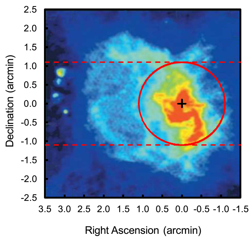
Figure 1: Map of the Galactic centre ($5^{\prime}\times 5^{\prime}$) at 6 cm (Yusef-Zadeh et al., 2000), indicating the the beam size of the Itapetinga radio telescope (red circle) and the scan direction (pointed red lines). The position of SgrA* is indicate by a black cross.

The method of observation was scans in right ascension, with 30 arcmin amplitude and 20 s duration. Only 24 arcmin were effectively utilized, the rest was lost during the inversion of the scan direction. During each scan 81 equally spaced data values, with integration time of $1/6$ s, were obtained. Each observation consisted of the average of 30 scans, preceded by a calibration; during an observing day, between 7 and 14 observations were obtained and averaged, always when the source was in elevation above $30^{\circ}$ and below $75^{\circ}$. The observations of SgrA* were alternated with similar observation of the HII region SgrB2, which was used as a quasi-simultaneous secondary calibrator.

The main problem in the detection of radio variability from SgrA* with single dish observation is the contribution of the continuum emission from the region surrounding this point source. As we show in Fig. 1, one scan with 24 arcmin amplitude and 2.2 arc min HPBW, detects not only SgrA* but part of the continuum complex SgrA. Since only SgrA* emission is variable, we used SgrA as an instantaneous calibrator, and as a result increased the variability detection capacity of our observations. To check the accuracy of this calibration and obtain a realistic value of the errors involved in the flux determination, we used a second calibrator: the strong HII region SgrB2 Main.

In order to separate the contribution of SgrA* from the surrounding SgrA emission, we first averaged all the observations from the year 2007, and adjusted three gaussians to the data: a point source with HPBW equal to the beam size (2.2 arc min), with two free parameters (peak flux density and central position) representing the average flux density of SgrA* during this period, and two other gaussians with completely free parameters. The result of the best fitting is presented in Table 1; in Fig. 2, we show the averaged data (dots), the adjusted gaussians and the residuals (observations minus model). The blue and the navy coloured regions in Fig. 1 are represented in Fig. 2 by the two strongest gaussians; the adjusted HPBWs match very well their angular sizes. The emission of SgrA* is represented by the smaller gaussian.

During the data reduction process, we also adjusted three gaussians to the observations, with the HPBW of each of them given in Table 1, maintaining constant their relative positions as well as the relative intensities of the two gaussians that represent the contribution of the SgrA complex. The free parameters were the position and intensity of the strongest gaussian, and the intensity of SgrA*.The flux density of SgrA*, calibrated with the SgrA complex, was obtained by dividing its observed flux density by the ratio of the flux densities of the strongest component of the SgrA complex and of its 2007 average value.

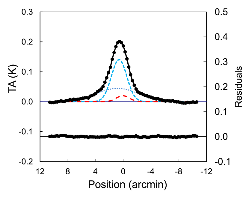
Figure 2: Averaged 7 mm observations (points) during 2007. The pointed and small broken lines represent the gaussian model for the SgrA complex while the large broken line represent the Gaussian contribution of SgrA*. The full line is the sum of the three component model.

The observations of SgrB2 Main, the quasi-instantaneous calibrator, were made with the same method as those of SgrA*, i.e. scans in right ascension with 30 arcmin amplitude and 20 s duration. The observations were made alternately with those of SgrA* and with the same integration time. As for SgrA, two gaussians were fitted to the averaged observations obtained in 2007, their parameters are presented in the last two rows of Table 1.

The flux density of SgrA* was also calibrated using the strongest component of SgrB2 Main and he difference of of the results of the two calibrations was taken as the measurement error.

Table 1: Parameters the Gaussian models of SgrA*, SgrA complex and SgrB2.

Source	Intensity (K)	HPBW (’)	$x_{0}$ (’)
SgrA*	0.020	2.2	0.06
SgrA (gaussian1)	0.141	2.59	0.59
SgrA(gaussian2)	0.044	7.30	0.80
SgrB2 (gaussian1)	0.167	2.52	0.00
SgrB2 (gaussian2)	0.015	8.45	0.85

3 Results and Discussion

Although interferometric observations provide flux density measurements with better error bars due to the higher angular resolution, single dish light curves can have better temporal resolution for variability studies, as a consequence of more available observation time. This is particularly important for SgrA*, because the previously detected periodicities are of monthly timescale and so, they need long time monitoring to be confirmed. Also, the large day-to-day variability at 22, 43 and 86 GHz, recently reported by Lu et al. (2011), needs a sequence of observations in consecutive days to be detected. This is the first time that SgrA* variability is studied using single dish observations and again, this was only possible because we used the emission of the SgrA complex as a simultaneous calibrator, as discussed in section 2. In Table 2 we show the values of the flux density for the first year of our monitoring. The values for the complete light curve are presented in the online version.

Table 2: Observations days of SgrA* in 2006

Date	JD-2450000	Flux Density	Error
		(Jy)	(Jy)
21-06-2006	3907.5	1.86	0.01
28-06-2006	3914.5	2.35	0.13
29-06-2006	3915.5	2.09	0.04
30-06-2006	3916.5	2.10	0.12
04-07-2006	3921.5	1.99	0.00
05-07-2006	3922.5	2.01	0.08
06-07-2006	3923.5	2.44	0.02
18-07-2006	3935.5	1.90	0.01
19-07-2006	3936.5	2.35	0.02
24-07-2006	3941.5	1.96	0.10
25-07-2006	3942.5	2.18	0.07
26-07-2006	3943.5	2.03	0.04
27-07-2006	3944.5	2.45	0.08
28-07-2006	3945.5	2.13	0.08
09-08-2006	3956.5	1.84	0.08
10-08-2006	3957.5	2.14	0.08
11-08-2006	3958.5	2.08	0.02
12-08-2006	3959.5	2.23	0.00
16-08-2006	3963.5	2.11	0.03
21-08-2006	3968.5	2.14	0.05
23-08-2006	3970.5	1.90	0.02

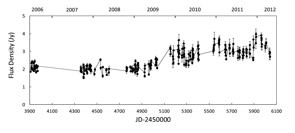
Figure 3: 7 mm light curve of SgrA*. The error bars represent the differences obtained using the two calibrators, SgrA complex and SgrB2 main

3.1 Variability

The results of six years monitoring of SgrA* at 7 mm are presented in Fig. 3. We detected an increase in the emission after the first semester of 2009; between 2007-2009 the average emission was $2.1\pm 0.2$ Jy, while it was $2.8\pm 0.2$ Jy in 2010 and $3.1\pm 0.2$ Jy in 2011. At the same time there was an increase in the amplitude of the variability, which had an average value of $1.1$ Jy in 2007-2009 (low phase) and $2.1$ Jy afterwards (high phase). The maximum flux density in our light curve was 4 Jy, value never reached at 7 mm, although Yusef-Zadeh et al. (2011) detected 3 Jy with the VLA before the beginning of our observations.

Coincidence in flux density during quasi-simultaneous observations with interferometric techniques, at the same frequency, shows the reliability of our results. In fact, Yusef-Zadeh et al. (2006), using the VLA for rapid variability studies, reported a 43 GHz flux density of $1.70\pm 0.10$ Jy on 2006 July 17, while we found $1.90\pm 0.01$ Jy on July 18. At other frequencies, Fish et al. (2011) found a flux density of $2.07\pm 0.15$ Jy at 1.3 cm on 2009 April 5, while for this day we found $2.21\pm 0.13$ Jy at 7 mm. Finally, we have 4 days data coincident with ATCA 3 mm observations (Li et al., 2009), which show the same variability pattern, as can be seen in Fig. 4. This is the first time that correlation between variability at these two radio frequencies is detected in SgrA*. The ATCA observations also revealed the existence of IDVs on 2006 August 13. When we looked at our data in a 10 min timescale, we found during the same day a dispersion higher than average; unfortunately, the large error bars of the observations for short integration times makes it difficult to detected these events without simultaneous interferometric observations.

In our single dish light curve we have 183 observations in consecutive days. We found day-to-day flux density variations larger than 0.5 Jy in 23 of them, only four times during the low state. In 6 opportunities, the day-to-day variations were even larger than 0.75 Jy. Similar variability was detected in 2007 at 43 GHz using VLBI observations, when SgrA* emission showed changes in flux density of $0.5$ Jy that coincided with two NIR flares (Kunneriath et al., 2010; Lu et al., 2011). Unfortunately, there are no infrared data for the epochs at which we detected strong daily variability. On the other hand, there are 45 consecutive days in which the flux density variation was smaller than our error bars. These events were present both before and after the rise in the light curve, being 16 detected before 2009 December.

In our monitoring program, we have 5 epochs with more than six consecutive days of observation, they are shown in Fig. 5. Day-to-day variability is present in some of them; the largest occurred in 2010 January, when the flux density changed from a minimum of $1.9\pm 0.2$ Jy in January 29 to a maximum of $3.7\pm 0.3$ Jy after 4 days. This happened at the beginning of the high phase in the light curve. Four months later, in 2010 June, the flux density slowly decreased from $3.2\pm 0.2$ Jy to $2.6\pm 0.1$ Jy during days 6 and 12.

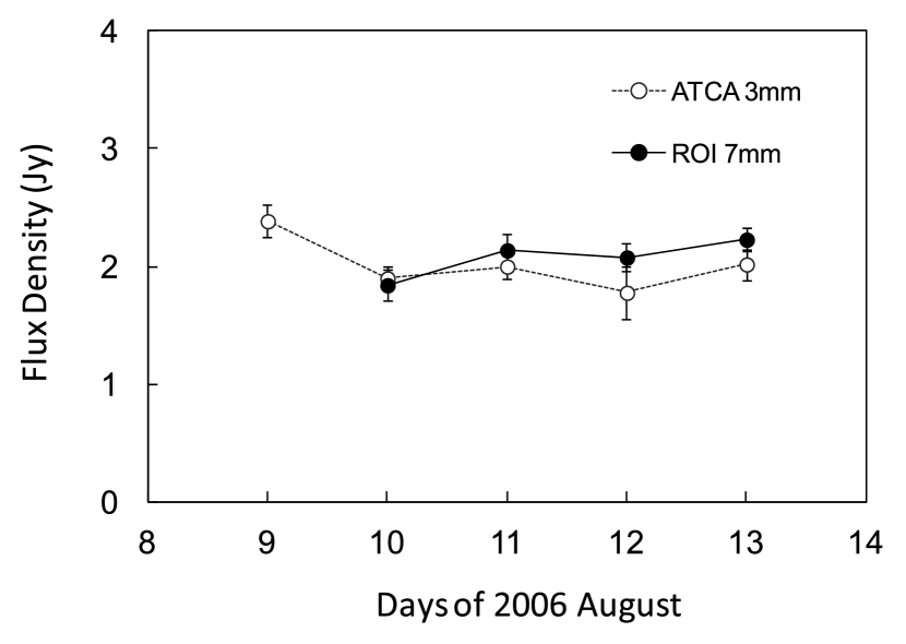
Figure 4: ATCA and Itapetinga simultaneous observations of SgrA*.

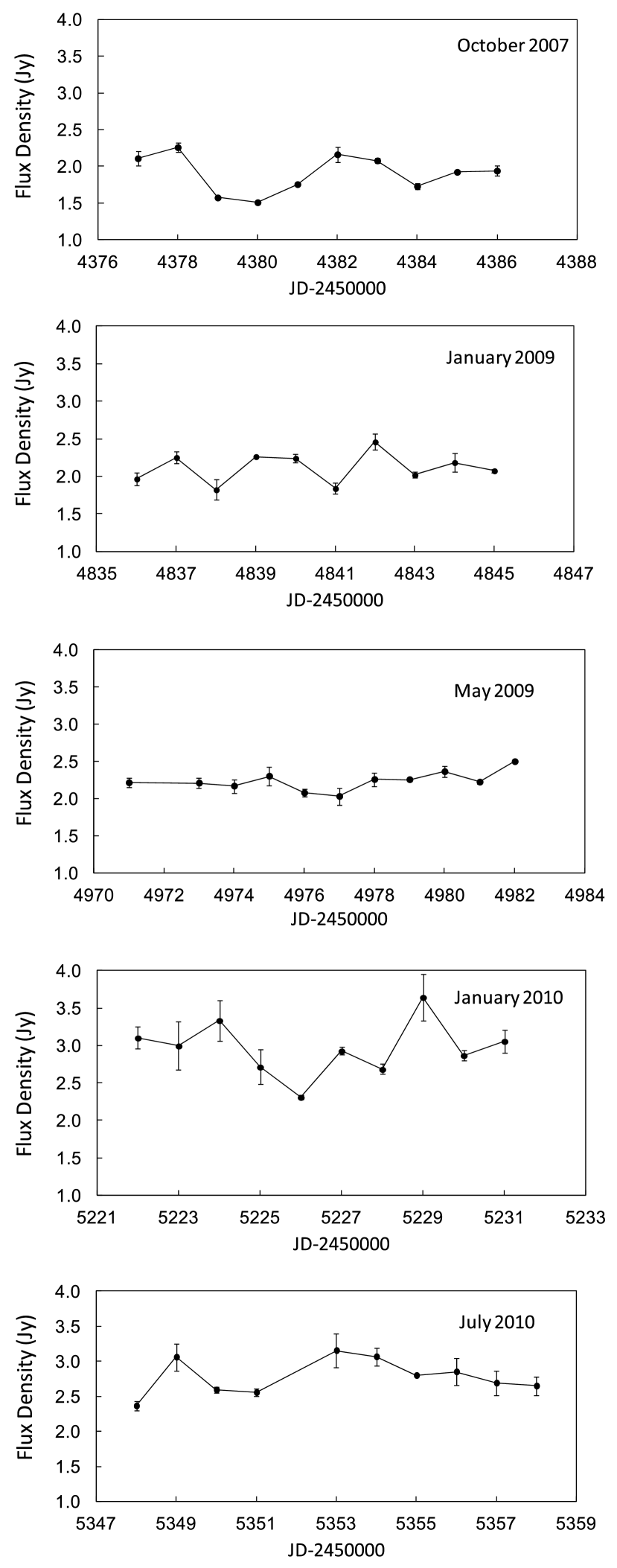
Figure 5: Light curve of SgrA* for five epochs with observations in more than six consecutive days.

The increase in the 7 mm flux density during the last years was also observed at other wavelengths. The RXTE (1.5-12) keV ASM light curve (Rossi X-Ray Time Explorer, All Sky Monitor) shows an increase in the SgrA* flux density by a factor of $2.5$ relative to its average value before 2010. SgrA* was never so intense at X-ray since the beginning of the ASM program. In the infrared, the K band intensity also showed an increase that started in 2008, after an intense flare detected in August 5 by the Very Large Telescope (Dodds-Eden et al., 2011).

We were able to determine the spectral index $\alpha$ $(S_{\nu}\propto\nu^{\alpha})$ between the 7 mm and H-band flux densities in two simultaneous observations. In 2006 June 24 and 27, the H-band flux densities were $4$ and $7$ mJy, respectively, (Bremer et al., 2011) while the 7 mm flux densities were $1.96\pm 0.01$ and $2.45\pm 0.05$ Jy respectively; between those days there was a monotonous rise in flux at 7mm. The IR-radio spectral index was -0.7 for both coincident days, which is compatible with the IR spectral index of $-0.6\pm 0.2$ found by Hornstein et al. (2007). This coincidence favours the idea that the emission could be produced by the the same non-thermal electron distribution (Yuan et al., 2003). We have also 7 mm and K-band simultaneous observations on 2006 June 21, which gave a spectral index of -1.1.

3.2 Periodicity

As it was already mentioned, two periods were previously reported in the SgrA* radio emission: 106 days, determined from 20 years of VLA observations at 22 GHz (Zhao et al., 2001), and 57 days found after 600 days of observations with the GBI at 2.3 GHz (Falcke, 1999). Our data set is not so long as the VLA database, but has better temporal resolution, while it is longer than the GBI monitoring but with worse temporal resolution. In other words, our light curve is irregularly sampled but without long gaps, which allows a more reliable statistical analysis.

To check the existence of possible periodicities we used the Structure Function Analysis and the Stellingwerf method. The intensity of the structure function (hereafter SF) is defined as $D(\tau)=\langle[I(t+\tau)-I(t)]^{2}\rangle$. This is a simple method to verify how much the intensity $I$ varies after a time delay $\tau$. If there is no characteristic timescale in the light curve, $D$ will have a random value for each $\tau$, and so there will be no maxima or minima in the structure function. Instead, if there is a typical timescale $\tau^{+}$ in the light curve, $D$ will be large when $\tau=\tau^{+}$ and appear as a maximum in the SF. This method is also useful to find periodicity, because if there is a period $P$, $D$ will have a low value when $\tau$ is equal to an integer number of periods, and this will result in minima in the SF.

The Stellingwerf method (Stellingwerf, 1978) is used to find periodicity in an irregularly sampled series. The test divides the sample in $m$ groups following the phase criterion:

$$\phi_{i}=\frac{t_{i}}{P}-\biggl{[}\frac{t_{i}}{P}\biggr{]}$$ (1)

where $\phi_{i}$ is the phase, $t_{i}$ is the observation time and $P$ is the guessed period. The brackets correspond to the integer part of the fraction. Each observation day of the sample has a value for the phase and it is grouped with other days with similar phases. The variable $\theta$ is defined as the ratio between the sum of the mean square deviation of the fluxes in each group, and the mean square deviation of the complete sample. If $P$ did not correspond to the real period, $\theta$ will be close to 1. If $P$ is indeed the period in the signal, there will be in the same group days with similar flux densities, and so, the sum of the group mean square deviation will be smaller than that of the complete sample. The number of groups is a free parameter, but higher values of $m$ provide deeper minima in the $\theta$ vs. $P$ curve. However, $m$ can not be too large, because we need a sufficient number of elements in each group to obtain a reliable statistics. We used $m=30$ for all tests in this work.

First, we applied both tests to the original light curve; the results are shown in Fig. 6 (a) and (b). Then, we applied the tests to the data after removing a third-order polynomial to discount the slow time variation; the results shown in Fig. 6 (c) and (d). This last procedure is similar to that used by Zhao et al. (2001).

In both cases we found several maxima and minima. To verify their significance and check if they are not consequence of sampling problems, we constructed an artificial light curve using random values for the flux density but with the same variability amplitude, for the days in which SgrA* was observed. The results of the statistical tests applied to this light curve are presented in Fig. 7. The range of the oscillations in the SF function lies between $-0.23$ and $+0.43$ of its mean value, which corresponds to $2.5$ and $4.0$ $\sigma$, respectively. We used these values to limit the significance of the maxima and minima in Fig. 6 (c), shown as red dashed lines. The only minimum deeper than this limit corresponds to $156\pm 10$ days, but marginal minima are present at the resonant $320\pm 10$ days period, and at $220\pm 10$ days, which could be resonant with the 106 day cycle reported by Zhao et al. (2001).

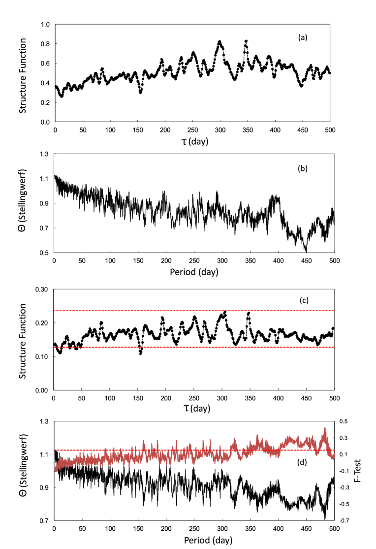
Figure 6: Statistical results for SgrA* 7 mm light curve: (a) and (b) SF and Stellingwerf results for the original light curve; (c) SF and (d) Stellingwerf and F-test results (in red) after a third-order polynomial was removed from the light curve. The red dashed lines represent the significance limit.

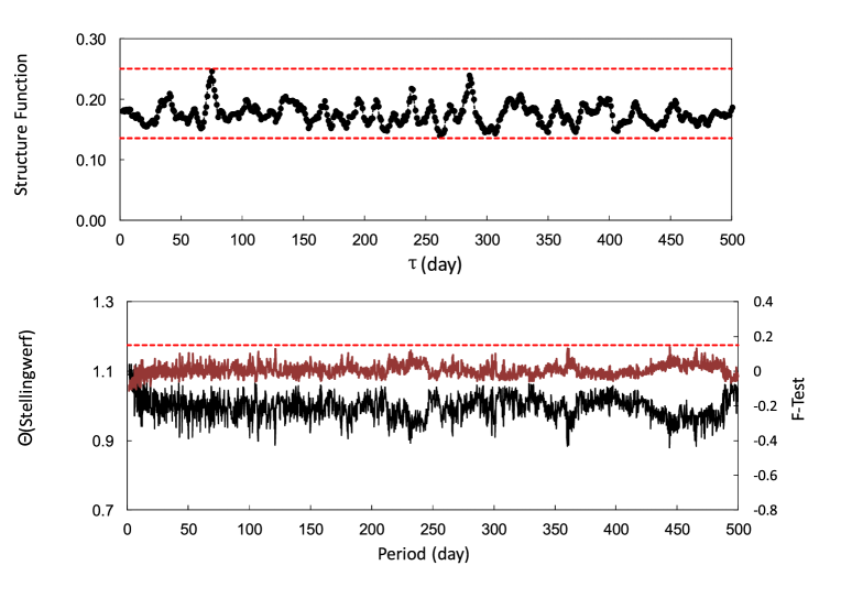
Figure 7: Statistical results for a random signal in the same days as those of our light curve. For the SF, the red dashed lines represent the extremes of the oscillations; for the Stellingwerf method the F-test function is included (in red), the dashed red line is the maximum value of this function

The significance of the Stellingwerf method results can be computed through the F-Test, developed by Kidger et al. (1992):

$$f=\frac{1-\Theta}{\Theta},$$ (2)

where $f>0.5$ indicates strong periodicity and $f<0.25$, the absence or weak periodicity. In fact, the $f$ test applied to the random light curve results shows always $f<0.15$. This value is represented as the red dashed line in Fig. 6 (d). We can see wide 156 and 320 days minima which seem to be significant ($f=0.27$), as well as several other very narrow minima, which we interpret as fluctuations. As discussed in Kidger et al. (1992), the Stellingwerf method can not reveal periods in a sampling smaller than six times the proposed period. In our light curve, this means periods longer than 350 days.

We conclude from the Structure Function and the Stelingwerf method that are two possible periods: $156\pm 10$ and $220\pm 10$ days that do not coincide with any of those previously reported: 57 days (Falcke, 1999) at 2.3 GHz and and 106 days (Zhao et al., 2001) at 22 GHz. However, we speculated if the existence of two beating periods could be the reason for the different results obtained by different authors. To check this hypothesis, we constructed artificial light curves as combination of two sine square functions, leaving their relative amplitudes as a free parameter and adding a random signal with amplitude similar to that of the periodic functions. We tried all possible combinations of 57, 106, 156, 212, 220 periods. We used 212 days because it is exactly a resonance of the 106 day cycle. Two combinations reproduced our statistical results: 156 and 212 days, and the 57 and 156 days; the amplitudes of the 156 days periodic sine square functions were 1.2 and 1.5 times larger than that of the 57 and 212 days periodic signals, respectively. The statistical tests are compared in Fig. 8. The 156 days minimum was not found by any combination of other periods, and the result of using 220 or 212 days period are very similar.

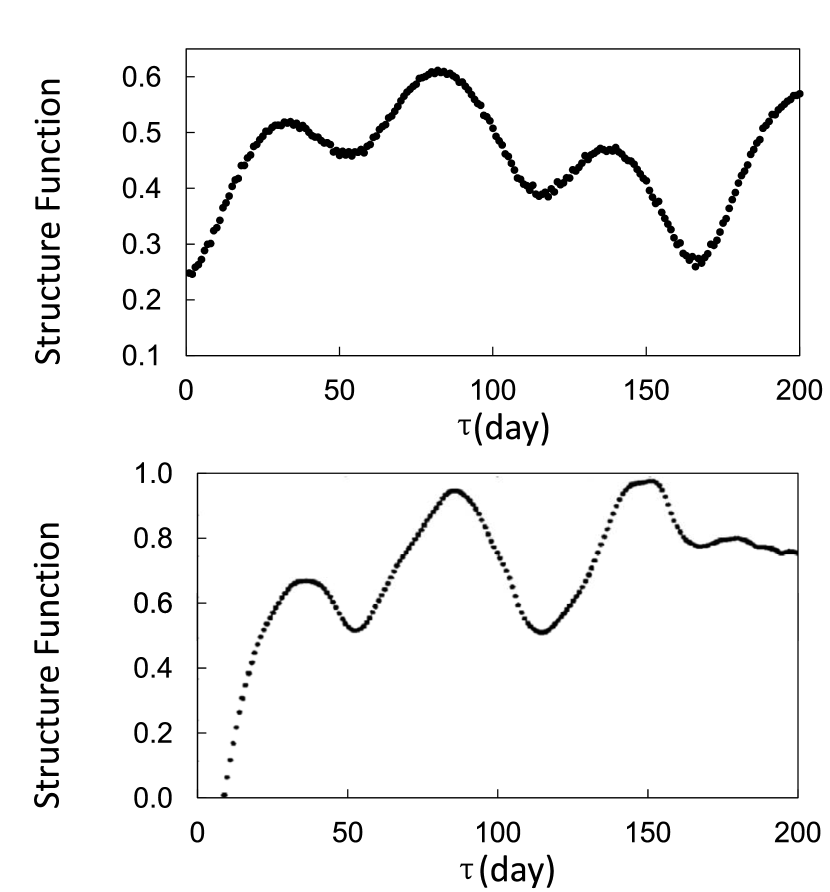
Figure 9: Top: SF results for the simulated two period light curve (57 and 156 days) with daily time resolution. Bottom: the SF results obtained by Falcke (1999) for the GBI monitoring at 2.3 GHz. The SF of the Falcke (1999) data are normalized by the highest peak.

The minimum that would correspond to the 57 days period did not appear in any of the combinations, even if this period was used in the input data. We believe that this could be a consequence of not having enough temporal resolution added to the existence of large amplitude short timescale fluctuations. Therefore, we repeated our calculations using our simulated light curve for the 57 and 156 days periods with daily data points, and in fact, the presence of the 57 days minimum can be seen in Fig. 9. It is important to notice that the SF of the simulated light curve is in very good agreement with the SF found by Falcke (1999) for the 2.3 GHz data and that the larger amplitude of the second peak seen in both SFs is a consequence of the existence of these two periodicities. This was not the case when the combination of 156 and 212 days periodic signals were used, even with daily resolution.

In other words, only the combination of 57 and 156 days reproduce both our statistical tests and Falcke’s. To verify the range of possible periods around 57 days that can still reproduce Fig. 8, we repeated the tests combining the 156 day period with different periods between 51 and 61 days. If the second period is smaller than 55, there is no minimum in the SF around 220 days. Otherwise, if the second period is larger than 59 days, the minimum in 156 days is not deep enough. This indicates that a periodic signal of of $57\pm 2$ days mixed with other of 156 days can reproduce the $156\pm 10$ and $220\pm 10$ minima revealed by our statistical tests.

Considering the existence of the $57\pm 2$ period, we can interpret the 106 day cycle reported by Zhao et al. (2001) as a resonance of that period. To check this hypothesis we modulated our light curve with a 106 day period, and compared the result with that of Zhao et al. (2001). We found a similar pattern for both cycles, but without the two large peaks on days 75 and 100 present in the 13 mm cycle. The peaks can be due to the low number of observation days in the VLA light curve.

Finally, we must mention that no periodicity was reported by Macquart & Bower (2006) for the VLA data obtained by Herrnstein et al. (2004). To understand that we calculated the SF for these data and we did not find any periodicity either. Again, the reason is that the VLA light curve has not enough time coverage to detect monthly periodicities.

3.3 The infalling ionized gas cloud

As presented in subsection 3.1, variability of SgrA* was detected at 7 mm in timescales of days and years. The latter consisted of a continuous increase in flux density that started in 2008, as can be seen in Fig.11, where the radio data are averaged in 60 days bins. Coincidently, Gillessen et al. (2012) detected a dense gas cloud that is moving in the direction of SgrA* in a highly eccentric orbit and will reach its minimum approach in 2013.5. The almost spherical cloud of 15 mas $(2\times 10^{15}$ cm) observed in Br$\gamma$ in 2008, is being tidally disrupted and in 2011 presented a tail elongated in the orbital direction of about 200 mas.

To investigate if the increase in the 7 mm flux density between 2008 and 2011 could be the result of the appearance of the disrupted tail, we calculated the flux density of an ionized optically thick cloud of temperature $T$ that subtends a solid angle $\Omega=\pi\theta^{2}$:

$$S_{\lambda}=\frac{2kT}{\lambda^{2}}\Omega$$ (3)

where $S_{\lambda}$ is the flux density at wavelength $\lambda$, and $k$ is the Boltzmann constant.

Assuming $T=10^{4}$ K and $\theta=150$ mas, the size of the observed tail, we obtain $S_{7\rm mm}=1$ Jy, in agreement with our observations. We could assume then that the increase in the observed 7 mm flux density between 2008 and 2011 corresponded to an increase in the solid angle $\Omega$. This increase seemed to stop around 2011, which could be interpreted as the cloud becoming optically thin at that epoch. Assuming the optical depth $\tau_{7\rm mm}=1$, we can calculate the emission measure $EM=n_{H}^{2}L$ of the cloud from:

$$\tau_{\lambda}=2\times 10^{-23}n_{H}^{2}L\frac{\lambda^{2}}{T^{3/2}}g_{ff}$$ (4)

For $T=10^{4}$ K, the Gaunt factor is $g_{ff}\sim 7$, and $EM=1.4\times 10^{28}$ cm^-5.

If we assume a density of $10^{7}$ cm^-3 for the cloud, as obtained from numerical simulations of the evolution of a disrupted cloud (Burkert et al., 2012), we obtained a length $L=1.4\times 10^{14}$ along the line of sight, showing that the tail in the orbital plane could be formed by a thin layer of gas.

If the 7 mm radio emission is due to free-free emission, we should expect a corresponding flux density in the IR, given by

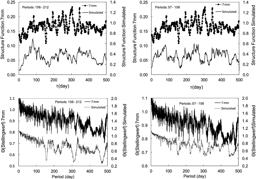
Figure 8: Comparison between the statistic results for the real (upper) and simulated (lower) light curves, for two different period combinations: 156 and 212 days (left) and 57-156 days (right). Top: Structure Function intensity, bottom: Stellingwerf method.

$$S_{\lambda}=5.4\times 10^{-16}T^{-0.5}g_{ff}(\lambda,T)\Omega EM\exp(\frac{-hc}{\lambda kT})\,\,\,\,{\rm Jy.}$$ (5)

For the IR, $g_{ff}(\lambda,T)\sim 1$; resulting for the $Ks$ band a flux density of $S_{Ks}\sim 0.057$ Jy. Although this value is much higher than any flux density detected in the SgrA* region, it must be noticed that it corresponds to an extended emission, therefore the signal should be diluted in an area of $150\times 150$ mas², which represents the size of the tail. Considering a pixel size of 13 or 27 mas per pixel, typical of the VLT data (Dodds-Eden et al., 2011; Gillessen et al., 2012) we obtain 0.43 and 1.8 mJy per pixel, which could have been overlooked in the data.

However, the increase in the amplitude of the fluctuations in timescales of days simultaneously with the increase in the total flux density that started around 2009, favours the hypothesis that is intrinsic to SgrA*. In fact,this relation between rms fluctuations and flux density was already detected in active galaxies and X-ray binaries at X-rays (Uttley & McHardy, 2001)and optical wavelengths (Gandhi, 2009) when they are in a luminous phase, which lead Heil et al. (2012) to claim that this can be an overall propriety of the accretion flow in compact sources. In the case of SgrA*, the increase in the accretion rate could be related to the influence of the infalling cloud or to the winds of faint stars during their periastron passage (Loeb, 2004), as those reported by Dodds-Eden et al. (2011).

4 Conclusion

In this paper we presented the results of single dish monitoring of SgrA* at 7 mm during a six year period. Great care was taken to separate the contribution of SgrA* from the surrounding emission, the latter used, together with the HII region SgrB2, as an instantaneous calibrator. The reliability of our results was verified by comparing them with interferometric observations at coincident epochs.

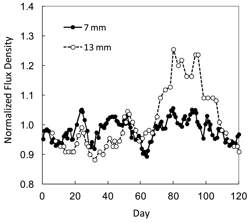
Figure 10: 106 day modulation of the 7 and the 13 mm light curves

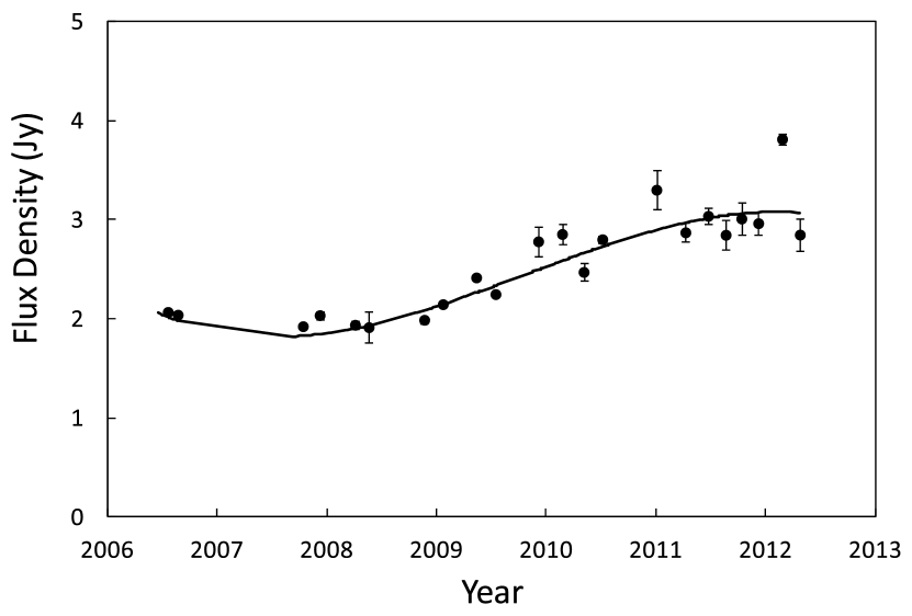
Figure 11: 7mm light curve with 60 days binning and the third order polynomial removed from the light curve (continue line)

During the observing campaign, several epochs with consecutive day observations allowed the study of variability in daily as well as longer timescales. The resulting light curve shows a slow variation in a timescale of years, a random component with shorter timescale and a day-to-day variability with large amplitude variations between two consecutive days.

We summarize the variability result as follow:

1. SgrA* emission at 7mm has been growing up through the years since 2008, this behaviour coincides with an increase in X-ray emission, and there is also some evidence of high activity in the infrared stating at the beginning of 2009.

2. SgrA* light curve presented episodes of high amplitude day-to-day variability that were more common in the high phase;

3. The variability at 7 mm showed the same pattern than that at 3 mm during four coincident days in 2006;

4. Simultaneous 7 mm and IR data revels that the radio-IR spectral index is similar to the IR spectral index, suggesting that the emission at that epoch was probably produced by the same electron population;

We investigate the possibility that the increase at 7 mm flux density that started in 2008 could be related to the appearance of a Br$\gamma$ emitting gaseous tail of tidally disrupted material, arising from the compact gas cloud that is falling towards SgrA* in a highly eccentric orbit (Gillessen et al., 2012). Even though it is possible to explain the 7 mm flux density increase as free-free emission from such a cloud, the predicted IR emission was not observed. However, the increase of the fluctuations together with the flux density at 7 mm , favours the intrinsic origin of this extra emission and is compatible with the rms/flux relation found in other compact sources (Uttley & McHardy, 2001).

In search for periodicity, the light curve was statistically analysed using the structure function and the Stellingwerf method. The result can be summarized as follows:

1. The statistical tests realized in this work revealed the existence of two minima: $156\pm 10$ and $220\pm 10$ days, but did not show any minima related to the 57 or 106 day periods reported by Falcke (1999) and Zhao et al. (2001).To test the reliability of our results we constructed an artificial light curve with random signals in the same observation days; no periodicity was found, showing that the existence of periodicity was not due to sampling effects.

2. We investigate if the divergence between the detected periods can be a consequence of the existence of two periodic signals. For that we simulated a light curve, as a combination of two quadratic sinusoidal functions, with data at the same observation days as those of our light curve, and verified which periods and relative amplitudes better reproduced our statistical results. We concluded that two combinations of periods can explain our statistical results: 156 plus 212 days, and 57 plus 156 days. The amplitudes of the 156 days periodic functions were 1.2 and 1.5 times larger than that of the 57 and 212 days periodic signals, respectively.

3. To test the influence of sampling in the detected periodicity, we constructed a simulated light curve for the 57 and 156 days periods with daily data points, using the same relative amplitudes as in the previous best test. The result of the structure function was in very good agreement with that found by Falcke (1999) for 2.3 GHz, which revealed the 57 day periodicity.

4. We also modulated our light curve with a 106 day period, to compare it with Zhao et al. (2001) results at 13 mm. The modulated light curves shows a similar pattern but without the two large peaks on days 75 and 100 of the cycle. This similarity can be explained as a consequence of a resonance of the 57 day period.

We conclude that two periodic signals added to a random component can reproduce statistical results similar to what it was obtained for the SgrA* emission. The combination of $156\pm 10$ and $57\pm 2$ day periodicity is what better explains our results. If real, these two periods may be explained by precession and/or nutation of a accretion disk. The precessing disk in SgrA* could be consequence of the the Bardeen-Peterson effect (Bardeen & Petterson, 1975), as discussed by Liu & Melia (2002). In fact, this process can lead to a hundred day period in the SgrA* radio emission (Caproni et al., 2004; Rockefeller et al., 2005).

References

- Abraham & Kokubun (1992) Abraham, Z., & Kokubun, F. 1992, A&A, 257, 831
- Baganoff et al. (2001) Baganoff, F. K., Bautz, M. W., Brandt, W. N., et al. 2001, Nature, 413, 45
- Baganoff et al. (2003) Baganoff, F. K., Maeda, Y., Morris, M., et al. 2003, ApJ, 591, 891
- Balick & Brown (1974) Balick, B., & Brown, R. L. 1974, ApJ, 194, 265
- Bremer et al. (2011) Bremer, M., Witzel, G., Eckart, A., et al. 2011, A&A, 532, A26
- Bardeen & Petterson (1975) Bardeen, J. M., & Petterson, J. A. 1975, ApJ, 195, L65
- Broderick & Loeb (2005) Broderick, A. E., & Loeb, A. 2005, MNRAS, 363, 353
- Broderick & Loeb (2006) Broderick, A. E., & Loeb, A. 2006, MNRAS, 367, 905
- Burkert et al. (2012) Burkert, A., Schartmann, M., Alig, C., et al. 2012, ApJ, 750, 58
- Caproni et al. (2004) Caproni, A., Mosquera Cuesta, H. J., & Abraham, Z. 2004, ApJ, 616, L99
- Coker et al. (1999) Coker, R., Melia, F., & Falcke, H. 1999, ApJ, 523, 642
- Cuadra et al. (2006) Cuadra, J., Nayakshin, S., Springel, V., & Di Matteo, T. 2006, Revista Mexicana de Astronomia y Astrofisica Conference Series, 26, 139
- Do et al. (2009) Do, T., Ghez, A. M., Morris, M. R., et al. 2009, ApJ, 691, 1021
- Dodds-Eden et al. (2011) Dodds-Eden, K., Gillessen, S., Fritz, T. K., et al. 2011, ApJ, 728, 37
- Doeleman et al. (2008) Doeleman, S. S., Weintroub, J., Rogers, A. E. E., et al. 2008, Nature, 455, 78
- Duschl & Lesch (1994) Duschl, W. J., & Lesch, H. 1994, A&A, 286, 431
- Eckart & Genzel (1996) Eckart, A., & Genzel, R. 1996, Nature, 383, 415
- Edelson & Krolik (1988) Edelson, R. A., & Krolik, J. H. 1988, ApJ, 333, 646
- Eisenhauer et al. (2003) Eisenhauer, F., Schödel, R., Genzel, R., et al. 2003, ApJ, 597, L121
- Falcke (1999) Falcke, H. 1999, The Central Parsecs of the Galaxy, 186, 113
- Falcke & Markoff (2000) Falcke, H., & Markoff, S. 2000, A&A, 362, 113
- Falcke et al. (2000) Falcke, H., Melia, F., & Agol, E. 2000, ApJ, 528, L13
- Fish et al. (2011) Fish, V. L., Doeleman, S. S., Beaudoin, C., et al. 2011, ApJ, 727, L36
- Gandhi (2009) Gandhi, P. 2009, ApJ, 697, L167
- Genzel et al. (2003) Genzel, R., Schödel, R., Ott, T., et al. 2003, Nature, 425, 934
- Ghez et al. (2004) Ghez, A. M., Wright, S. A., Matthews, K., et al. 2004, ApJ, 601, L159
- Gillessen et al. (2009) Gillessen, S., Eisenhauer, F., Trippe, S., et al. 2009, ApJ, 692, 1075
- Gillessen et al. (2012) Gillessen, S., Genzel, R., Fritz, T. K., et al. 2012, Nature, 481, 51
- Heil et al. (2012) Heil, L. M., Vaughan, S., & Uttley, P. 2012, MNRAS, 422, 2620
- Herrnstein et al. (2004) Herrnstein, R. M., Zhao, J.-H., Bower, G. C., & Goss, W. M. 2004, AJ, 127, 3399
- Hornstein et al. (2007) Hornstein, S. D., Matthews, K., Ghez, A. M., et al. 2007, ApJ, 667, 900
- Jolley & Kuncic (2008) Jolley, E. J. D., & Kuncic, Z. 2008, ApJ, 676, 351
- Kidger et al. (1992) Kidger, M., Takalo, L., & Sillanpaa, A. 1992, A&A, 264, 32
- Kuncic & Bicknell (2004) Kuncic, Z., & Bicknell, G. V. 2004, ApJ, 616, 669
- Kuncic & Bicknell (2007) Kuncic, Z., & Bicknell, G. V. 2007, Ap&SS, 311, 127
- Kunneriath et al. (2010) Kunneriath, D., Witzel, G., Eckart, A., et al. 2010, A&A, 517, A46
- Li et al. (2009) Li, J., Shen, Z.-Q., Miyazaki, A., et al. 2009, ApJ, 700, 417
- Liu & Melia (2002) Liu, S., & Melia, F. 2002, ApJ, 573, L23
- Loeb (2004) Loeb, A. 2004, MNRAS, 350, 725
- Lu et al. (2008) Lu, R.-S., Krichbaum, T. P., Eckart, A., et al. 2008, Journal of Physics Conference Series, 131, 012059
- Lu et al. (2011) Lu, R.-S., Krichbaum, T. P., Eckart, A., et al. 2011, A&A, 525, A76
- Macquart & Bower (2006) Macquart, J.-P., & Bower, G. C. 2006, ApJ, 641, 302
- Markoff et al. (2007) Markoff, S., Bower, G. C., & Falcke, H. 2007, MNRAS, 379, 1519
- Melia (1992) Melia, F. 1992, ApJ, 387, L25
- Melia (1994) Melia, F. 1994, ApJ, 426, 577
- Melia & Falcke (2001) Melia, F., & Falcke, H. 2001, ARA&A, 39, 309
- Melo et al. (2009) Melo, I., Tomášik, B., Torrieri, G., et al. 2009, Phys. Rev. C, 80, 024904
- Menten et al. (1997) Menten, K. M., Reid, M. J., Eckart, A., & Genzel, R. 1997, ApJ, 475, L111
- Meyer et al. (2008) Meyer, L., Do, T., Ghez, A., et al. 2008, ApJ, 688, L17
- Mościbrodzka et al. (2006) Mościbrodzka, M., Das, T. K., & Czerny, B. 2006, MNRAS, 370, 219
- Narayan et al. (1998) Narayan, R., Mahadevan, R., Grindlay, J. E., Popham, R. G., & Gammie, C. 1998, ApJ, 492, 554
- Prescher & Melia (2005) Prescher, M., & Melia, F. 2005, ApJ, 632, 1048
- Rockefeller et al. (2005) Rockefeller, G., Fryer, C. L., & Melia, F. 2005, ApJ, 635, 336
- Schödel et al. (2002) Schödel, R., Ott, T., Genzel, R., et al. 2002, Nature, 419, 694
- Stellingwerf (1978) Stellingwerf, R. F. 1978, ApJ, 224, 953
- Uttley & McHardy (2001) Uttley, P., & McHardy, I. M. 2001, MNRAS, 323, L26
- van der Laan (1966) van der Laan, H. 1966, Nature, 211, 1131
- Yuan et al. (2003) Yuan, F., Quataert, E., & Narayan, R. 2003, ApJ, 598, 301
- Yuan et al. (2002) Yuan, F., Markoff, S., & Falcke, H. 2002, A&A, 383, 854
- Yusef-Zadeh et al. (2000) Yusef-Zadeh, F., Melia, F., & Wardle, M. 2000, Science, 287, 85
- Yusef-Zadeh et al. (2006) Yusef-Zadeh, F., Roberts, D., Wardle, M., Heinke, C. O., & Bower, G. C. 2006, ApJ, 650, 189
- Yusef-Zadeh et al. (2008) Yusef-Zadeh, F., Wardle, M., Heinke, C., et al. 2008, ApJ, 682, 361
- Yusef-Zadeh et al. (2011) Yusef-Zadeh, F., Wardle, M., Miller -Jones, J. C. A., et al. 2011, ApJ, 729, 44
- Zhao et al. (2001) Zhao, J.-H., Bower, G. C., & Goss, W. M. 2001, ApJ, 547, L29
- Zhao et al. (1992) Zhao, J.-H., Goss, W. M., Lo, K.-Y., & Ekers, R. D. 1992, Relationships Between Active Galactic Nuclei and Starburst Galaxies, 31, 295