Study of a degenerate dipolar Fermi gas of ¹⁶¹Dy atoms

Abstract

We study properties of a single-component (spin polarized) degenerate dipolar Fermi gas of ¹⁶¹Dy atoms using a hydrodynamic description. Under axially-symmetric trapping we suggest reduced one- (1D) and two-dimensional (2D) description of the same for cigar and disk shapes, respectively. In addition to a complete numerical solution of the hydrodynamic model we also consider a variational approximation of the same. For a trapped system under appropriate conditions, the variational approximation as well as the reduced 1D and 2D models are found to yield results for shape, size and chemical potential of the system in agreement with the full numerical solution of the three-dimensional (3D) model. For the uniform system we consider anisotropic sound propagation in 3D. An analytical result for anisotropic sound propagation in uniform dipolar degenerate Fermi gas is found to be in agreement with results of numerical simulation in 3D.

1 Introduction

After the experimental realization of Bose-Einstein condensate (BEC) of ⁵²Cr [1, 2], ¹⁶⁴Dy [3], and ¹⁶⁸Er [4] atoms with large magnetic dipolar interaction, there have been renewed interest in the study of cold atoms, both theoretically and experimentally. The anisotropic long-range dipolar interaction acting in all partial waves in these atoms is basically different from isotropic short-range S-wave interaction acting in nondipolar atoms. Polar bosonic molecules with much larger permanent electric dipole moment are also candidates for possible BEC experiments [5]. Dipolar BECs have novel distinct properties. Due to the anisotropic dipolar interaction, the stability of a dipolar BEC depends on the scattering length as well as the trap geometry [2, 6, 7]. The shock and sound waves also propagate anisotropically in a dipolar BEC [8, 9]. Anisotropic collapse has been observed and studied in a dipolar BEC of ⁵²Cr atoms [10]. Anisotropic rotons [11] and anisotropic critical superfluid velocity [12] have been suggested and studied in dipolar BECs. Distinct stable checkerboard, stripe, and star configurations in dipolar BECs have been identified in a two-dimensional (2D) optical lattice as stable Mott insulator [13] as well as superfluid soliton [14] states. Anisotropic solitons in 2D have also been suggested in dipolar BECs [15]. A new possibility of studying universal properties of dipolar BECs at unitarity has been suggested [16].

After the realization of BEC of alkali-metal atoms, degenerate nondipolar gas of fermionic ⁶Li [17], ⁴⁰K [18], and ⁸⁷Sr [19] atoms were observed. Later, superfluid states of paired ⁶Li [20] and ⁴⁰K [21] Fermi atoms have been investigated. More recently a degenerate dipolar gas of fermionic ¹⁶¹Dy atoms with large magnetic dipole moment has been created and studied [22]. Realization of quantum degeneracy in ¹⁶¹Dy atoms should be considered as a doorway for the study of anisotropic superfluidity in dipolar fermions. Fermionic polar molecules, such as ⁴⁰K⁸⁷Rb, of large permanent electric dipole moment are also considered for this purpose [23]. The ⁴⁰K⁸⁷Rb molecule in the singlet rovibrational ground state has an electric dipole moment of 0.6 Debye, thus leading to a dipolar interaction larger than in the case of ¹⁶¹Dy atoms by more than an order of magnitude [1]. One advantage of studying the effect of dipolar interaction in a degenerate dipolar Fermi gas over that in a dipolar BEC is the remarkable stability of the degenerate Fermi gas. A BEC is usually fragile or short-lived for many experiments due to three-body loss through molecule formation. The three-body loss is highly suppressed in a degenerate Fermi gas due to Pauli repulsion among identical fermions. On the other hand a theoretical study of a BEC is much simpler than that of a degenerate Fermi gas [24] due to the existence of a simple order parameter and a simple mean-field Gross-Pitaevskii equation in the former case.

A microscopic description of a degenerate Fermi gas is complicated due to the difficulties with the antisymmetrization of a many-fermion system and finding an appropriate simple order parameter. Drastic approximations are often necessary to achieve this goal for fermions. There have been several different theoretical descriptions for a degenerate nondipolar Fermi gas [25]. There have also been a few studies of the degenerate dipolar Fermi gas employing different types of approximations [26]. However, for a description of some macroscopic observables of a degenerate Fermi gas, a simple hydrodynamic description [27] often seems appropriate which does not require a precise antisymmetrization of the dynamics [24, 28, 29]. The effect of antisymmetrization is included approximately via an appropriate energy or Lagrangian density. A minimization of the energy leads to a well-founded variational approximation [30]. An Euler-Lagrange equation derived from such a Lagrangian provides further improvement over the variational results. Here we present a description of the degenerate spin polarized Fermi gas based on such a hydrodynamic model [27, 28].

The present theoretical formulation for the degenerate dipolar Fermi gas starts in section 2.1 with the standard equations of classical hydrodynamics [27] with the appropriate equation of state including the kinetic energy of fermions filling the Fermi sea and the dipolar interaction among them. The equivalent of the Thomas-Fermi (TF) approximation for the dipolar gas is obtained by setting the velocity field equal to zero in the hydrodynamic equations. An equivalent classical energy density is written using the local-density approximation (LDA) [24]. A quantum pressure term is then introduced in the LDA energy density. With such a quantum pressure term, a nonlinear Schrödinger-type equation is derived for the density of fermions. For a moderate number of fermions (greater than 100 or so), the quantum pressure term is negligibly small and hence has insignificant effect on the result. However, the inclusion of the quantum pressure term allows one to write a dynamical equation for fermions in the form of a nonlinear Schrödinger equation to study the dynamics. The LDA or the TF approximation, on the other hand, allows only the investigation of static properties of the system. For example, these approximations cannot be used to study the sound propagation dynamics in fermions as in section 3.2. In section 2.2, we present a Gaussian variational approximation for the problem described by the LDA energy density. In section 2.3, simplified models are derived in reduced dimensions, appropriate for cigar and disk shapes of the degenerate dipolar gas when there is a strong trap in radial or in axial directions, respectively. In section 2.4, using the hydrodynamic model, we obtain an analytic expression for the anisotropic sound velocity in the degenerate dipolar gas. In section 3.1, we present numerical results for stationary properties $-$ shape, size, and chemical potential $-$ of a trapped degenerate Fermi gas of ¹⁶¹Dy atoms, and compare with results from appropriate models in reduced dimensions and variational approximation. In section 3.2, the anisotropic sound propagation in an infinite dipolar degenerate gas is demonstrated numerically and the velocities so obtained are compared with the analytical results of section 2 D. Finally, in section IV we present a summary of our study.

2 Analytical Consideration

2.1 Hydrodynamic Model

The normal one-component Fermi gas can be in the collisionless regime where collision is rare or in the collisional hydrodynamic regime where frequent collision due to the dipolar interaction allow the system to settle to local equilibrium, where the system can be described by simple hydrodynamic equation rather than a detailed multi-particle description. Here we consider the system in such a configuration. A semi-quantitative estimate for the validity of a hydrodynamic description is given by the condition that relaxation time $\tau_{R}$ is small compared to the time scale $1/\omega$ defined by average trap frequency $\omega$ [8, 9]. For contact interaction this condition can be expressed in terms of the scattering length to measure the strength of atomic interaction [31]. The strength of dipolar interaction is usually measured in terms of the convenient length $L_{d}\equiv 3a_{dd}=\mu_{0}\bar{\mu}^{2}m/(4\pi\hbar^{2})$, where $\bar{\mu}$ is the magnetic moment of an atom of mass $m$ and $\mu_{0}$ the permeability of free space. Using this length scale to measure dipolar interaction, the condition for the validity of hydrodynamic description can be expressed as [9, 31]

$$(\omega\tau_{R})^{-1}\approx\left(N^{1/3}\frac{L_{d}}{a_{\mathrm{ho}}}\right)^{2}F\left(\frac{T}{T_{F}}\right)>1,$$ (1)

where $N$ is the number of atoms, $a_{\mathrm{ho}}=\sqrt{\hbar/(m\omega)}$ the oscillator length, $T$ the temperature, $T_{F}$ the Fermi temperature and $F(x)$ an universal function and can be taken of the order of unity [31] under experimental conditions. Hence for sufficently large $N$ and/or sufficiently small $a_{\mathrm{ho}}$ the system should enter the hydrodynamic regime. For ¹⁶¹Dy atoms of magnetic moment $10\mu_{B}$ with $\mu_{B}$ the Bohr magneton, the length $L_{d}\equiv 3a_{dd}\approx 3\times 130a_{0}$ where $a_{0}$ is the Bohr radius and for an oscillator length $a_{\mathrm{ho}}=0.25$ $\mu$m and $N=5000$ the system is already in the hydrodynamic regime. For polar Fermi molecule ⁴⁰K⁸⁷Rb of electric dipole moment $d=0.566$ Debye in the singlet rovibrational ground state [23], the length $L_{d}=md^{2}/(4\pi\hbar^{2}\epsilon_{0})\approx 3\times 2000a_{0}$ [1], where $\epsilon_{0}$ is the permitivity of free space, and the system should enter the hydrodynamic regime with larger $a_{\mathrm{ho}}=1$ $\mu$m (weaker trap) and much smaller $N$ of few hundreds.

At sufficiently low temperature the normal Fermi gas enters the degenerate phase. Most macroscopic properties, like shape, density, chemical potential, sound propagation etc., of this system can be described by the Landau hydrodynamical equations [27]. A velocity field is introduced as the gradient of a velocity potential $\Phi$ of flow, usually related to phase of the order parameter, by ${\bf v}({\bf r},t)=\nabla\Phi({\bf r},t),$ subject to the irrotational condition $\nabla\times{\bf v}({\bf r},t)=0$. The continuity and the flow equations are then given by [27]

$$\frac{\partial n({\bf r},t)}{\partial t}+\nabla\cdot[n({\bf r},t)\bf v({\bf r},t)]=0,$$ (2)

$$m\frac{\partial\bf v(\bf r,t)}{\partial t}+\nabla\left[\frac{m{{\bf v(r},t)}^{2}}{2}+\mu(n,{\bf r})+V({\bf r})\right]=0,$$ (3)

where $n({\bf r},t)$ is density at space point $\bf r$ and time $t$, $V(\bf r)$ is an external trap, usually taken as

$$V({\bf r})=\frac{1}{2}m\omega^{2}(\nu^{2}\rho^{2}+\lambda^{2}z^{2}),$$ (4)

with $\omega$ the trap frequency and $\nu$ and $\lambda$ are anisotropy parameters. The bulk chemical potential $\mu(n,\bf r)$ is determined by the equation of state of the uniform Fermi gas of dipolar atoms and is given by

$$\mu(n,{\bf r})=\frac{\hbar^{2}[6\pi^{2}n({\bf r})]^{2/3}}{2m}+\int d{\bf r^{\prime}}n({\bf r^{\prime}})U_{dd}({\bf r-r^{\prime}}),$$ (5)

where the first term on the right-hand side (rhs) is the Fermi energy $E_{F}\equiv{\hbar^{2}(6\pi^{2}n)^{2/3}}/({2m})$ [24] and the last term is the contribution from dipolar interaction energy [28], with $U_{dd}(\bf r-r^{\prime})$ is the dipolar potential.

The hydrodynamic description is valid for a macroscopic observable with its characteristic excitation wave-length $\lambda$ much larger than the healing length [24]. A safe condition to satisfy this criterion is to take the wave length to be much larger than de Broglie wavelength at the Fermi surface, i.e., [24, 32]

$$\lambda\gg 2\pi/k_{F}$$ (6)

with Fermi momentum $k_{F}$ defined by $E_{F}=\hbar^{2}k_{F}^{2}/2m$. Truly speaking, a degenerate Fermi gas may not be fully irrotational and allows rotational components in the velocity field, not allowed in the present hydrodynamic formulation. This fact should influence only the rotational properties [24] of the degenerate Fermi gas not considered in this paper. We also assume the absence of any velocity dependent frictional force.

An approximate TF profile for density can now be obtained by setting velocity ${\bf v}=0$ in (3), when [24]

$$\mu(n,{\bf r})+V({\bf r})=\mu_{0}^{\mathrm{TF}},$$ (7)

where $\mu_{0}^{\mathrm{TF}}$ is the chemical potential of the trapped gas. When (7) is solved subject to the appropriate normalization condition, we obtain both the chemical potential $\mu_{0}^{\mathrm{TF}}$ and the density $n(\bf r)$.

There is an equivalent description of the trapped degenerate Fermi gas in the LDA, based on the assumption that, locally the dipolar Fermi gas would behave like a uniform gas, so that the energy density can be written as the energy of the uniform system times the local density [24]. For the degenerate dipolar Fermi system, the classical energy density per particle is given by [26, 28]

$${\cal E}_{\mathrm{cl}}({\bf r}) =\frac{3}{5}\frac{\hbar^{2}}{2m}(6\pi^{2}N)^{2/3}[n({\bf r})]^{5/3}+V({\bf r})n({\bf r})$$ (8)

$$+N\frac{1}{2}\int d{\bf r^{\prime}}n({\bf r})n({\bf r^{\prime}})U_{dd}({\bf r-r^{\prime}}),$$

where $n(\bf r)$ is the density of fermions normalized as $\int d{\bf r}n({\bf r})=1$. The first term on the rhs of (8) is the total kinetic energy of the spin polarized fermions filling all levels up to the Fermi sea, the second term is energy in the trap, and the third term describes the dipolar interaction. A minimization of the classical energy (8) leads to the TF condition (7).

As the degenerate Fermi gas is a quantum system, a quantum pressure term when included in (8) yields the following expression for net energy density

$${\cal E}({\bf r})=\frac{\hbar^{2}}{8m}|\nabla_{\bf r}\sqrt{n(\bf r)}|^{2}+{\cal E}_{\mathrm{cl}}({\bf r}).$$ (9)

This gradient correction term [33] to the TF energy density (8) takes into account the additional kinetic energy due to spatial variation of density (near the surface). Such a surface term was first considered by von Weiszäcker [34, 35, 36] in the description a large nuclei. Previous descriptions of a degenerate Fermi gas considered different coefficients in this term [25, 33]. The energy density (9) has successfully used in many problems of Fermi gas [35, 36, 37, 38].

With the Lagrangian density ${\cal L}({\bf r})={\cal E}({\bf r})-\mu_{0}n(\bf r)$ the Euler-Lagrange equation is given by [37]

$$\mu_{0}\sqrt{n{(\bf r)}} =\biggr{[}-\frac{\hbar^{2}\nabla^{2}}{8m}+V({\bf r})+\frac{\hbar^{2}}{2m}[6\pi^{2}Nn({\bf r})]^{2/3}$$ (10)

$$+N\int U_{dd}({\bf r-r^{\prime}})n({\bf r^{\prime}})d{\bf r^{\prime}}\biggr{]}\sqrt{n({\bf r})},$$

with $\mu_{0}$ the chemical potential. The derivarive term in (10) term contributes much less than the dominant “Fermi energy” term $\hbar^{2}[6\pi^{2}Nn({\bf r})]^{2/3}/(2m)$ and its neglect leads to the TF relation (7). The dipolar interaction in (10) is taken as $U_{dd}({\bf R})=3a_{dd}\hbar^{2}(1-3\cos^{2}\theta)$ $/(mR^{3}),$ $\quad{\bf R=r-r^{\prime}}$ where $\theta$ is the angle between the $\bf R$ and the polarization direction $z.$

The condition (1) refers to the validity of a hydrodynamic description of the system ($\bf v\neq 0$) [9, 31]. A reliable stationary description obtained using (10) for $\bf v=0$, of density and other macroscopic properties, such as sound velocity, as considered in this paper, can be obtained for a smaller number of fermions consistent with condition (6) [24, 32], provided the contribution of the kinetic energy term $\hbar^{2}[6\pi^{2}Nn({\bf r})]^{2/3}/(2m)$ in (10) is much larger than that of other terms.

It is convenient to write a dimensionless form of (10) with the potential (4) as

$$\mu_{0}\sqrt{n{(\bf r)}} =\biggr{[}-\frac{\nabla^{2}}{8}+\frac{1}{2}(\nu^{2}\rho^{2}+\lambda^{2}z^{2})+\frac{1}{2}[6\pi^{2}Nn({\bf r})]^{2/3}$$ (11)

$$+3a_{dd}N\int\frac{1-3\cos^{2}\theta}{R^{3}}n({\bf r^{\prime}})d{\bf r^{\prime}}\biggr{]}\sqrt{n({\bf r})},$$

where energy, length and density are expressed in units of $\hbar\omega$, $l_{0}=\sqrt{\hbar/m\omega}$ and $l_{0}^{-3}$.

2.2 Variational Approximation

The energy density corresponding to the dimensionless equation (11) can be written as

$${\cal E}({\bf r}) =\frac{1}{8}|\nabla_{\bf r}\sqrt{n(\bf r)}|^{2}+\frac{3a_{dd}N}{2}\int d{\bf r^{\prime}}n({\bf r})n({\bf r^{\prime}})\frac{1-3\cos^{2}\theta}{R^{3}}$$ (12)

$$+\frac{1}{2}(\nu^{2}\rho^{2}+\lambda^{2}z^{2})n({\bf r})+\frac{3}{10}(6\pi^{2}N)^{2/3}[n({\bf r})]^{5/3}.$$

A variational approximation for the problem can be obtained with the following Gaussian ansatz for density [30]

$$n({\bf r})=\frac{1}{\pi^{3/2}w_{\rho}^{2}w_{z}}\exp\left[-\frac{\rho^{2}}{w_{\rho}^{2}}-\frac{z^{2}}{w_{z}^{2}}\right],$$ (13)

where $w_{\rho}$ and $w_{z}$ are the variational widths along radial $\rho$ and axial $z$ directions. With this density, the effective energy per particle of the system $E=\int d{\bf r}{\cal E}({\bf r})$ is

$$E =\frac{1}{8}\left[\frac{1}{w_{\rho}^{2}}+\frac{1}{2w_{z}^{2}}\right]+\left[\frac{\nu^{2}w_{\rho}^{2}}{2}+\frac{\lambda^{2}w_{z}^{2}}{4}\right]$$ (14)

$$-\frac{Na_{dd}f(\kappa)}{\sqrt{2\pi}w_{\rho}^{2}w_{z}}+\sqrt{\frac{3}{5}}\frac{9(6\pi^{2}N)^{2/3}}{50\pi w_{\rho}^{4/3}w_{z}^{2/3}},$$

where $\kappa=w_{\rho}/w_{z}$ and

$$f(\kappa)=\frac{1+2\kappa^{2}}{1-\kappa^{2}}-\frac{3\kappa^{2}\mbox{tanh}^{-1}\sqrt{1-\kappa^{2}}}{(1-\kappa^{2})^{{3/2}}}.$$ (15)

The variational equations are obtained by minimizing the energy (14) by $\partial E/\partial w_{z}=\partial E/\partial w_{\rho}=0$ [2, 30]:

$${w_{\rho}}\nu^{2} =\frac{1}{4w_{\rho}^{3}}-\frac{a_{dd}}{\sqrt{2\pi}}\frac{Ng(\kappa)}{w_{\rho}^{3}w_{z}}+\sqrt{\frac{3}{5}}\frac{6(6\pi^{2}N)^{2/3}}{25\pi w_{z}^{2/3}w_{\rho}^{7/3}},$$ (16)

$${w}_{z}\lambda^{2} =\frac{1}{4w_{z}^{3}}-\frac{a_{dd}}{\sqrt{2\pi}}\frac{2Nh(\kappa)}{w_{\rho}^{2}w_{z}^{2}}+\sqrt{\frac{3}{5}}\frac{6(6\pi^{2}N)^{2/3}}{25\pi w_{z}^{5/3}w_{\rho}^{4/3}},$$ (17)

where

$$g(\kappa)=\frac{2-7\kappa^{2}-4\kappa^{4}}{(1-\kappa^{2})^{2}}+\frac{9\kappa^{4}\mbox{tanh}^{-1}\sqrt{1-\kappa^{2}}}{(1-\kappa^{2})^{5/2}},$$ (18)

$$h(\kappa)=\frac{1+10\kappa^{2}-2\kappa^{4}}{(1-\kappa^{2})^{2}}-\frac{9\kappa^{2}\mbox{tanh}^{-1}\sqrt{1-\kappa^{2}}}{(1-\kappa^{2})^{5/2}}.$$ (19)

The chemical potential $\mu_{0}$ of the system per particle is

$$\mu_{0} =\frac{1}{8}\left[\frac{1}{w_{\rho}^{2}}+\frac{1}{2w_{z}^{2}}\right]+\left[\frac{\nu^{2}w_{\rho}^{2}}{2}+\frac{\lambda^{2}w_{z}^{2}}{4}\right]$$ (20)

$$-\frac{2Na_{dd}f(\kappa)}{\sqrt{2\pi}w_{\rho}^{2}w_{z}}+\sqrt{\frac{5}{3}}\frac{9(6\pi^{2}N)^{2/3}}{50\pi w_{\rho}^{4/3}w_{z}^{2/3}}.$$

2.3 Approximate density for cigar and disk shapes

In many situations of experimental interest, the Fermi gas could be subject to a strong trap either in the polarization $z$ direction or in the transverse radial $\rho$ plane. The system then has a one-dimensional (1D) cigar or 2D disk shape, respectively. In such cases simplified equations in lower dimensions could be very useful [39].

First we consider the reduced 1D equation for a cigar shape. We assume that there is a strong trap in the $x-y$ plane and that the density in this plane is given by the Gaussian ground state [39] $n(\rho)=\exp(-\rho^{2}/d_{\rho}^{2})/(\sqrt{\pi}d_{\rho}),d_{\rho}=\sqrt{1/(2\nu)}$ of the trap $\nu^{2}\rho^{2}/2$, so that the 3D density $n({\bf r})$ satisfies

$$\sqrt{n({\bf r})}\equiv\sqrt{n(\rho)}\sqrt{n(z)}=\frac{\sqrt{n(z)}}{\sqrt{\pi}d_{\rho}}\exp\left[-\frac{\rho^{2}}{2d_{\rho}^{2}}\right].$$ (21)

Substituting this density in (11), and multiplying this equation by the corresponding Gaussian $\sqrt{n(\rho)}$ and integrating out the $\rho$ dependence we obtain the reduced 1D equation [40, 41]

$$\mu_{1D}\sqrt{n(z)}=\biggr{[}-\frac{\partial_{z}^{2}}{8}+\frac{\lambda^{2}z^{2}}{2}+\frac{3[6Nn(z)]^{2/3}}{10d_{\rho}^{4/3}}$$

$$+\frac{2a_{dd}N}{d_{\rho}^{2}}\int_{-\infty}^{\infty}\frac{dk_{z}}{2\pi}e^{ik_{z}z}n(k_{z})s_{1D}\left(\frac{k_{z}d_{\rho}}{\sqrt{2}}\right)\biggr{]}\sqrt{n(z)},$$ (22)

$$s_{1D}(\zeta)=\int_{0}^{\infty}du\frac{2\zeta^{2}-u}{u+\zeta^{2}}e^{-u},$$ (23)

where $n(k_{z})=\int_{-\infty}^{\infty}e^{-ik_{z}z}n(z)dz,$ and $\mu_{1D}$ is the chemical potential. An approximate variational solution of (2.3) is possible with the following ansatz for density [41] $n(z)={1}/({\sqrt{\pi}w_{z}})\exp[-{z^{2}}/{w_{z}^{2}}],$ while the width $w_{z}$ is determined by solving (17) with $w_{\rho}=d_{\rho}$ and $\kappa=d_{\rho}/w_{z}$.

Next we consider the reduced 2D equation suitable for a disk shape with a strong axial trap. The dipolar Fermi gas is assumed to be in the ground state [39] $n(z)=\exp(-z^{2}/d_{z}^{2})/(\sqrt{\pi}d_{z}),d_{z}=\sqrt{1/(2\lambda)}$, of the axial trap $\lambda^{2}z^{2}/2$ and the 3D density can be approximated as

$$\sqrt{n({\bf r})}\equiv\sqrt{n(\rho)}\sqrt{n(z)}=\frac{\sqrt{n(\rho)}}{\pi^{1/4}\sqrt{d_{z}}}\exp\left[-\frac{z^{2}}{2d_{z}^{2}}\right].$$ (24)

Using this ansatz in (11), and multiplying by the corresponding Gaussian $\sqrt{n(z)}$ and integrating out the $z$ dependence we get the effective 2D equation [41, 42]

$$\mu_{2D}\sqrt{n(\rho)}=\biggr{[}-\frac{\nabla^{2}_{\rho}}{8}+\frac{1}{2}\nu^{2}\rho^{2}+\sqrt{\frac{3}{5}}\frac{[6Nn(\rho)]^{2/3}\pi}{2d_{z}^{2/3}}$$

$$+\frac{4\pi a_{dd}N}{\sqrt{2\pi}d_{z}}\int\frac{d^{2}k_{\rho}}{(2\pi)^{2}}e^{i{\bf k_{\rho}.\rho}}n({\bf k_{\rho}})h_{2D}\left(\frac{k_{\rho}d_{z}}{\sqrt{2}}\right)\biggr{]}\sqrt{n(\rho)},$$ (25)

where $n({\bf k_{\rho}})=\int e^{i\bf k_{\rho}.\rho}n(\rho)d^{2}\rho,h_{2D}(\xi)=2-3\sqrt{\pi}\xi e^{\xi^{2}}[1-\mbox{erf}(\xi)].$ An approximate variational solution of (25) is possible with the following ansatz for density [41] $n(\rho)={1}/{(\pi w_{\rho}^{2})}\exp[-{\rho^{2}}{w_{\rho}^{2}}],$ while the width $w_{\rho}$ is determined by solving (16) with $w_{z}=d_{z}$ and $\kappa=w_{\rho}/d_{z}$.

2.4 Sound propagation in a uniform Fermi gas

To find the sound velocity in a uniform Fermi gas, we evaluate the Bogoliubov spectrum using the linearized hydrodynamic equations. We consider a stationary Fermi gas in a box with periodic boundary condition with the trap $V$ fixing just the allowed plane wave solution. Then (3), after the inclusion of the gradient term of (9), reduces to

$$-\frac{\hbar^{2}\nabla^{2}\sqrt{n({\bf r},t)}}{8m\sqrt{n({\bf r},t)}}+\mu(n,{\bf r})+m\frac{\partial\Phi({\bf r},t)}{\partial t}=0.$$ (26)

Now we allow small perturbation in $n$ and $\Phi$ around their equilibrium values $n_{0}$ and $\Phi_{0}$ by $n({\bf r},t)\approx n_{0}+\bar{n}({\bf r},t)$ and $\Phi({\bf r},t)\approx\Phi_{0}+\bar{\Phi}({\bf r},t)$, then (2) leads to

$$\frac{\partial\bar{n}({\bf r},t)}{\partial t}+n_{0}\nabla^{2}\bar{\Phi}({\bf r},t)=0.$$ (27)

In (26), we need to use $\sqrt{n({\bf r},t)}\approx\sqrt{n_{0}}+\bar{n}({\bf r},t)/(2\sqrt{n_{0}})$ and $[n({\bf r},t)]^{2/3}\approx n_{0}^{2/3}+2\bar{n}({\bf r},t)/(3{n_{0}}^{1/3})$, while $\mu(n,{\bf r})\approx\tilde{\mu}_{0}+\bar{\mu}(n,{\bf r})$ with

$$\bar{\mu}(n,{\bf r})=\frac{\hbar^{2}(6\pi^{2})^{2/3}\bar{n}}{3mn_{0}^{1/3}}+\int d{\bf r^{\prime}}\bar{n}({\bf r^{\prime}},t)U_{dd}({\bf r-r^{\prime}}),$$ (28)

where $\tilde{\mu}_{0}$ is the stationary value of $\mu$. Then (26) leads to

$$-\frac{\hbar^{2}\nabla^{2}{\bar{n}({\bf r},t)}}{16mn_{0}}+\bar{\mu}(n,{\bf r})+m\frac{\partial\bar{\Phi}({\bf r},t)}{\partial t}=0.$$ (29)

Assuming the perturbations $\bar{n}$ and $\bar{\Phi}$ in plane-wave forms $\bar{n}=\bar{n}_{0}\exp[i({\bf k\cdot r})-\omega t]$ and $\bar{\Phi}=\bar{\Phi}_{0}\exp[i({\bf k\cdot r})-\omega t],$ $\bar{\mu}$ has the form $\bar{\mu}=\bar{n}_{0}\bar{\mu}_{0}\exp[i({\bf k\cdot r})-\omega t]$ with

$$\bar{\mu}_{0}=\frac{\hbar^{2}(6\pi^{2})^{2/3}}{3mn_{0}^{1/3}}+\frac{4\pi a_{dd}\hbar^{2}}{m}(3\cos^{2}\theta-1),$$ (30)

where $\theta$ is the angle between the propagation direction and polarization direction $z$, and the last term in (30) is just the Fourier transform of the dipolar potential. Then (27) and (29) become:

$$-i\omega\bar{n}_{0}-n_{0}k^{2}\bar{\Phi}_{0}=0,$$ (31)

$$\left[\frac{\hbar^{2}k^{2}}{16mn_{0}}+\bar{\mu}_{0}\right]\bar{n}_{0}-i\omega m\bar{\Phi}_{0}=0.$$ (32)

The condition of existence of the solution to this set of equations leads to the Bogoliubov spectrum

$$\epsilon_{k}\equiv\hbar\omega=\sqrt{\frac{\hbar^{2}k^{2}}{4m}\left[\frac{\hbar^{2}k^{2}}{4m}+4n_{0}\bar{\mu}_{0}\right]}.$$ (33)

The sound velocity, defined as $c_{s}(\theta)=\lim_{k\to 0}(\epsilon_{k}/\hbar k)$ for a uniform dipolar Fermi gas can be written as

$$c_{s}(\theta)=\sqrt{\frac{v_{F}^{2}}{3}+\frac{4\pi n_{0}a_{dd}\hbar^{2}}{m^{2}}(3\cos^{2}\theta-1)},$$ (34)

where $v_{F}\equiv\hbar k_{F}/m=\hbar(6\pi^{2}n_{0})^{1/3}/m$ is the Fermi velocity. For a nondipolar Fermi gas ($a_{dd}=0$), (34) leads to the well-known velocity of $v_{F}/\sqrt{3}$ [24, 29].

The angle-dependent second term under the square root in (34) is responsible for anisotropic sound velocity. Specifically, for $\theta>54.73^{\circ}$ degrees, this term is negative corresponding to a decrease in sound velocity. For large dipolar interaction, for $\theta$ greater than a critical value and for large density $n_{0}$ the sound velocity could be imaginary corresponding to no propagation. However, in this study we shall only consider moderate values of density and dipolar interaction, that allow anisotropic sound propagation in all directions.

3 Numerical Results

3.1 Stationary properties of trapped dipolar Fermi gas

For a trapped 3D Fermi system we solve (11) numerically after discretization [43]. The divergence of the dipolar term at short distances has been handled by treating this term in momentum ($\bf k$) space [6]. For numerical calculation in section 3.1, we consider a degenerate Fermi gas of ¹⁶¹Dy atoms with $a_{dd}\approx 130a_{0}$ and employ the oscillator length $l_{0}=1$ $\mu$m.

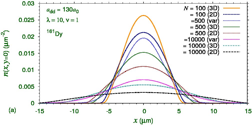
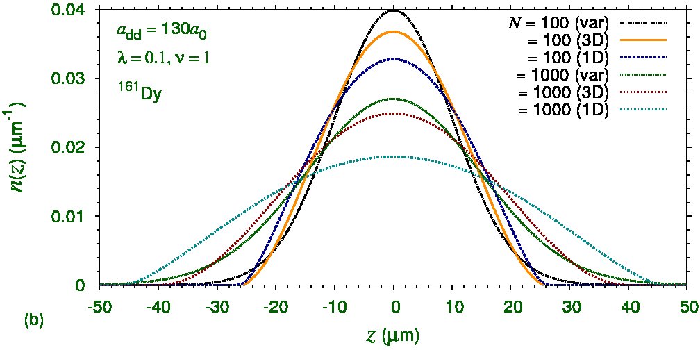
Figure 1: (a) Radial density of a disk-shaped Fermi gas of ¹⁶¹Dy atoms in $x-y$ plane $n(x,y=0)=\int_{-\infty}^{\infty}dzn(x,y=0,z)$ from the 3D (11) for $\nu=1,\lambda=10$ compared with its variational (var) approximation and the solution of the reduced 2D (25) for $N=100,500,10000$. (b) Axial density of a cigar-shaped Fermi gas of ¹⁶¹Dy atoms along polarization $z$ axis $n(z)=\int_{-\infty}^{\infty}\int_{-\infty}^{\infty}dxdyn(x,y,z)$ from the 3D (11) for $\nu=1,\lambda=0.1$ compared with its variational (var) approximation and the solution of the reduced 1D (2.3) for $N=100,1000$.

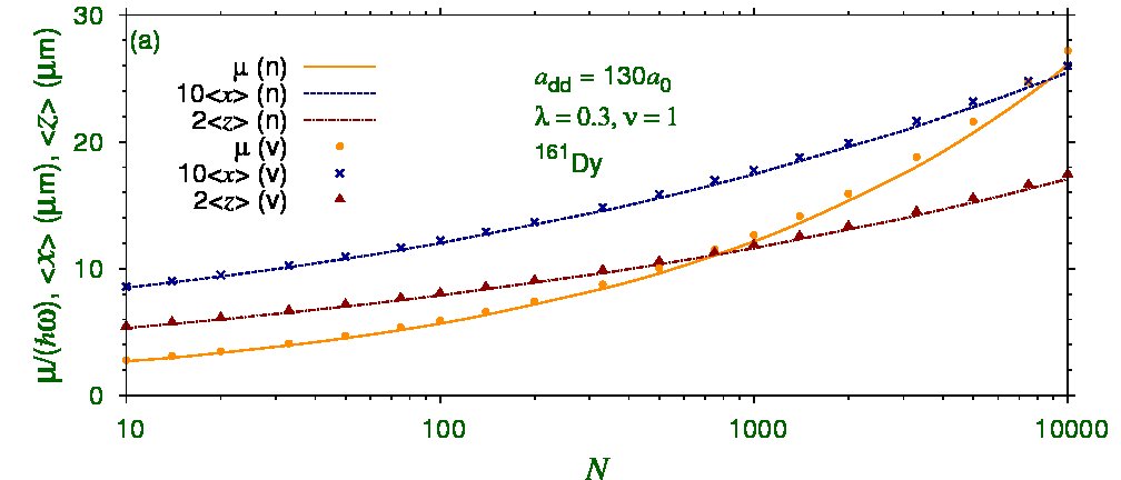
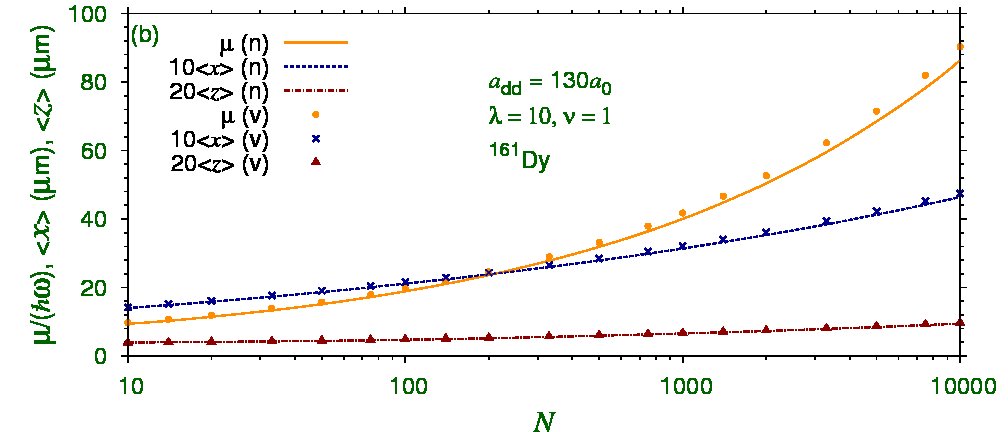
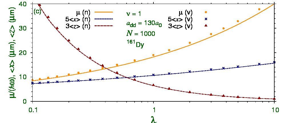
Figure 2: (a) Reduced chemical potential $\mu/(\hbar\omega)$, and rms sizes $\langle x\rangle$, and $\langle z\rangle$ of a cigar-shaped Fermi gas of ¹⁶¹Dy atoms with $\nu=1,\lambda=0.3$ versus $N$ from a numerical (n) solution of the 3D (11) and variational (v) approximation [ (16), (17) and (20)]. (b) The same for a disk-shaped gas with $\nu=1,\lambda=10$. (c) The same for the trapped Fermi gas of 1000 ¹⁶¹Dy atoms versus the parameter $\lambda$ with $\nu=1$ from a numerical solution of (11) and variational approximation.

The anisotropic dipolar interaction is partially attractive in certain angles and repulsive in others and contributes very little in a spherically symmetric trap. The dipolar interaction contributes attractively in the cigar-shaped configuration along the polarization $z$ direction and repulsively in the disk-shaped configuration perpendicular to the polarization $z$ direction. Hence we will mostly consider the degenerate dipolar Fermi gas in cigar and disk shapes. The 3D model (11) is very strongly nonlinear with nonlinearity ${\cal N}=(6\pi^{2}N)^{2/3}/2$, leading to large nonlinearities of ${\cal N}=760$ and 3526 for $N=1000$ and 10000, respectively.

First, we compare the results of the reduced 2D density $n(x,y)$ of a disk-shaped degenerate Fermi gas of ¹⁶¹Dy atoms with $\lambda=10,\nu=1$ as obtained from the 3D and 2D models (11) and (25), respectively, and from the variational approximation to the 3D model. The reduced 2D density $n(x,y)$ is defined by $n(\rho)\equiv n(x,y)=\int_{-\infty}^{\infty}dzn(x,y,z)$. In figure 1 (a) we plot the reduced 2D density along $x$ axis $n(x,y=0)$ for different $N$. Next, we compare the results of reduced 1D density $n(z)$ of a cigar-shaped degenerate Fermi gas of ¹⁶¹Dy atoms with $\lambda=0.1,\nu=1$ as obtained from the 3D and 1D models (11) and (2.3), respectively, and from the variational approximation to the 3D model. The reduced 1D density $n(z)$ is defined by $n(z)=\int_{-\infty}^{\infty}dx\int_{-\infty}^{\infty}dyn(x,y,z)$. In figure 1 (b) we plot the reduced 1D density along $z$ axis $n(z)$ for different $N$. From figure 1 we find that in both cigar and disk shapes the 1D and 2D models perform fairly well, even for large nonlinearities, when compared with the results of the full 3D model. To see if the condition (6) is satisfied by the shapes in figure 1, we can use the TF estimate for $k_{F}$ of a trapped degenerate Fermi gas [24]: $k_{F}\approx(48N)^{1/6}/l_{0}$. For $100<N<10000$, as in figure 1, the de Broglie wave length at the Fermi surface is $2\pi/k_{F}\approx l_{0}$ . The shapes and sizes in figure 1 are much larger than this value, consistent with the condition (6).

Next we consider a cigar-shaped degenerate Fermi system of ¹⁶¹Dy atoms with trap parameters $\nu=1,\lambda=0.3$. In figure 2 (a) we plot the numerical and variational results for the chemical potential $\mu$ and rms sizes $\langle x\rangle$ and $\langle z\rangle$ of this system for $10<N<10000$. In figure 2 (b) we plot the same for a disk-shaped degenerate Fermi system with trap parameters $\nu=1,\lambda=10$. Finally, in figure 2 (c) we plot the same quantities for $N=1000$ versus the trap anisotropy $\lambda$ for $\nu=1$. In all cases the variational results are in good agreement with the 3D model. For medium to small number ($N<10000$) of trapped ¹⁶¹Dy atoms as considered here and also of experimental interest, the effect of the dipolar term in Eq. (11) (the last term in this equation) is small compared to the Fermi energy term (the last but one term there). Hence the effect of the dipolar term in figures 2 is small. The plots in these figures only change by less than about two to four percent if we set $a_{dd}=0$.

3.2 Anisotropic sound propagation in uniform dipolar Fermi gas

The hydrodynamic analytical result for sound velocity (34) in a uniform dipolar Fermi gas shows a clear anisotropy through the angle $\theta$ between the propagation direction $\bf r$ and the polarization direction $z$. In this expression for sound velocity there are two competing terms under the square root. The first term $v_{F}^{2}/3$ involving the Fermi velocity is isotropic and proportional to $n_{0}^{2/3}$ whereas the second term proportional to dipolar interaction is anisotropic and proportional to density $n_{0}$. The anisotropy in sound velocity $c_{s}(\theta)$ will manifest strongly for large strength $a_{dd}$ and for large $n_{0}$ as the anisotropic dipolar term in (34) will increase more rapidly with $n_{0}$ than the isotropic term. In figure 3 (a) we plot the sound velocity $c_{s}(\theta)$ for angles $\theta=0$ and $\pi$ as a function of density $n_{0}$ for a degenerate Fermi gas with $a_{dd}=130a_{0}$ (¹⁶¹Dy atom) and $2000a_{0}$ (polar ⁴⁰K-⁸⁷Rb molecules in the singlet rovibrational ground state [1]) using the analytical result (34). The sound velocity for nondipolar atoms ($a_{dd}=0$) is also plotted. From this plot we find that the anisotropy in sound propagation as measured by the difference $[c_{s}(0)-c_{s}(\pi/2)]$ is sizable only for a relatively large density $n_{0}=10^{15}$ cm^-3 for ¹⁶¹Dy atoms. However, for polar ⁴⁰K-⁸⁷Rb molecules the anisotropy is appreciable for a relatively low density of $n_{0}=10^{13}$ cm^-3. From figure 3 (a) we see that for ⁴⁰K-⁸⁷Rb molecules, the sound velocity is imaginary for $\theta=0$ for a density of about $n_{0}=5\times 10^{13}$ cm^-3.

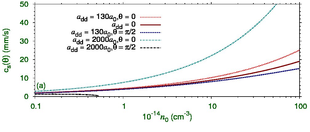
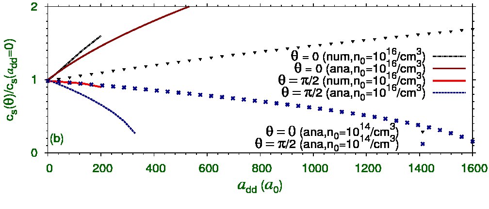
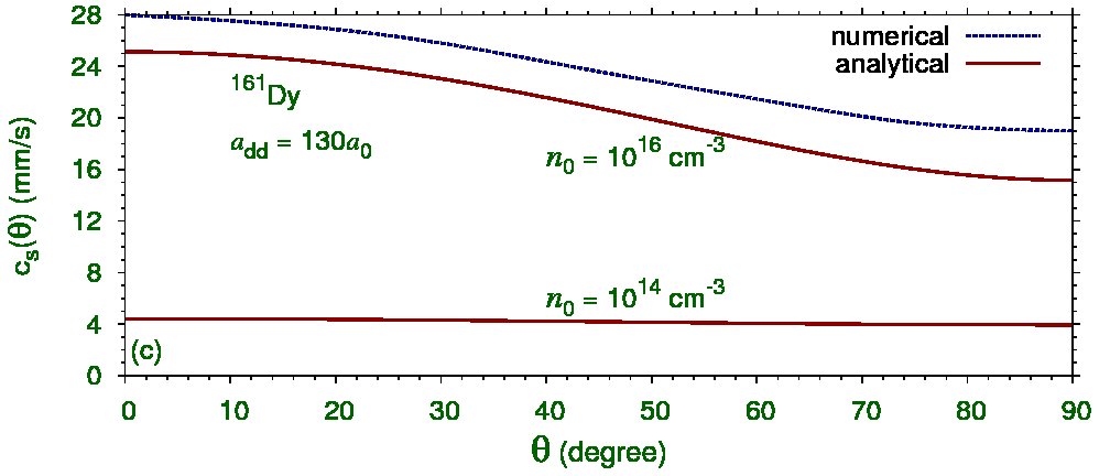
Figure 3: (a) The analytical sound velocity $c_{s}(\theta)$ given by (34) in axial $z$ ($\theta=0$) and radial $\rho$ ($\theta=\pi/2$) directions versus density $n_{0}$ for $a_{dd}=130a_{0}$ and 2000$a_{0}$ as well as the velocity for $a_{dd}=0$. (b) The analytical (ana) sound velocity $c_{s}(\theta)$ in axial $z$ ($\theta=0$) and radial $\rho$ ($\theta=\pi/2$) directions versus $a_{dd}$ compared with the results of numerical simulation (num). (c) The analytical sound velocity $c_{s}(\theta)$ versus polar angle $\theta$ compared with the results of numerical simulation.

To study sound propagation, the present stationary (static) 3D model (11) is generalized to include time variation by replacing $\mu$ by the usual time derivative $i\hbar\partial/\partial t$. Consequently, the infinite dipolar Fermi gas satisfies the following Galilei-invariant equation [37]

$$i\hbar\frac{\partial}{\partial t}\sqrt{n_{0}{(\bf r)}}=\biggr{[}-\frac{\hbar^{2}\nabla^{2}}{2(2m)}+2V({\bf r})+2\frac{\hbar^{2}}{2m}[6\pi^{2}n_{0}({\bf r})]^{2/3}$$

$$+12a_{dd}\frac{\hbar^{2}}{2m}\int\frac{1-3\cos^{2}\theta}{R^{3}}n_{0}({\bf r^{\prime}})d{\bf r^{\prime}}\biggr{]}\sqrt{n_{0}({\bf r})},$$ (35)

where density $n_{0}({\bf r})=Nn({\bf r})$ is not normalizable for infinite hydrodynamics. Equation (3.2) is consistent [37] with the time-dependent hydrodynamic equation (3) after the inclusion of the gradient correction term [33].

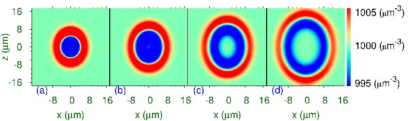
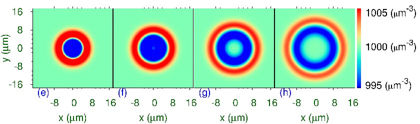
Figure 4: The contour plot of 3D density in $x-z$ plane $n_{0}(x,y=0,z)$ during sound propagation on a background density $n_{0}=10^{3}$ $\mu$m^-3 of a degenerate dipolar ¹⁶¹Dy gas with $a_{dd}=130a_{0}$ at times $t=$ (a) $0.15t_{0}$, (b) $0.2t_{0}$, (c) $0.25t_{0}$, and (d) $0.3t_{0}$ ($t_{0}=0.005$ s). The contour plot of 3D density in $x-y$ plane $n_{0}(x,y,z=0)$ during the same sound propagation at times (e) $0.15t_{0}$, (f) $0.2t_{0}$, (g) $0.25t_{0}$, and (h) $0.3t_{0}$.

The anisotropy of the dipolar interaction would be prominent at low to medium density for large dipolar interaction. To illustrate the anisotropic sound propagation we will consider two examples: ¹⁶¹Dy atoms at a medium density of 10¹⁵ cm^-3 and the polar molecules ⁴⁰K-⁸⁷Rb at the low density of 10¹³ cm^-3. First we consider the numerical simulation of sound propagation in the infinite ¹⁶¹Dy gas ($a_{dd}=130a_{0}$) at a background density of $n_{0}=10^{3}$ $\mu$m${}^{-3}=10^{15}$ cm^-3. The numerical simulation is initiated with a 3D Gaussian pulse at the center of the uniform 3D background density given by $n_{0}({\bf r})=(10^{3}+10^{2}e^{-r^{2}/2w^{2}})$ $\mu$m^-3, $w=2$ $\mu$m, subject to a weak expulsive Gaussian potential $V({\bf r})=0.00001e^{-r^{2}/2w^{2}}$ $\mu$m^-2. With this initial condition (3.2) is solved by real-time propagation [43] to study sound waves. An ellipsoid-like sound wave front is found to emerge outwards upon time propagation. From a numerical study of this wave front the sound velocity in different directions is calculated.

Typical anisotropic sound propagation in a ¹⁶¹Dy degenerate gas of density 10¹⁵ cm^-3 is shown in figure 4. The sound propagation is illustrated via contour plots of 3D density $n_{0}(x,y,0)$ in the $x-y$ plane and of density $n_{0}(x,0,z)$ in the $x-z$ plane. In figures 4 (a), (b), (c), and (d), to illustrate the anisotropic sound propagation in the $x-z$ plane, we show the contour plot of $n_{0}(x,0,z)$ at times $t=0.15t_{0},0.2t_{0},0.25t_{0}$ and $0.3t_{0}$, respectively, with $t_{0}=2ml_{0}^{2}/\hbar^{2}\approx 0.005$ s the time scale and $l_{0}=1$ $\mu$m the length scale used in the numerical solution of (3.2). However, the propagation in the radial $x-y$ plane is isotropic. This isotropic sound propagation is shown in figures 4 (e), (f), (g), and (h) via the contour plot of $n_{0}(x,y,0)$ at times $t=0.15t_{0},0.2t_{0},0.25t_{0}$ and $0.3t_{0}$, respectively. A clean wave front of high density is identified in these contour plots encompassing a region of low density $-$ a typical panorama in sound propagation.

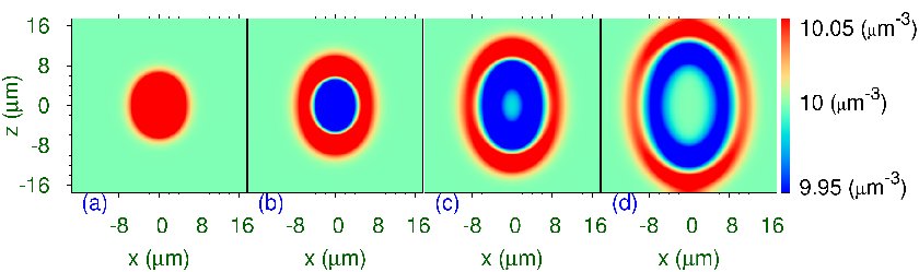
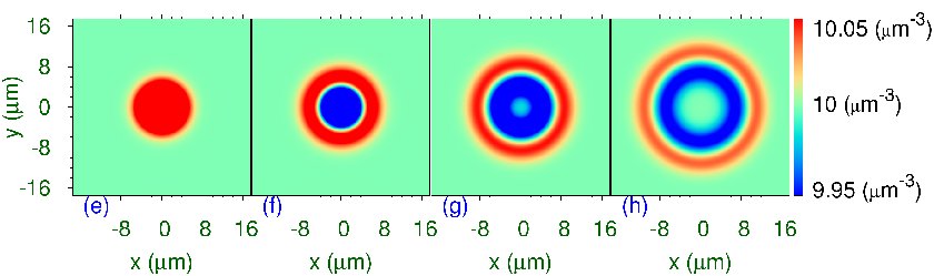
Figure 5: The contour plot of 3D density in $x-z$ plane $n_{0}(x,y=0,z)$ during sound propagation on a background density $n_{0}=10$ $\mu$m^-3 of a degenerate dipolar molecular ⁴⁰K-⁸⁷Rb gas with $a_{dd}=1000a_{0}$ at times $t=$ (a) $0.2t_{0}$, (b) $0.5t_{0}$, (c) $0.8t_{0}$, and (d) $1.1t_{0}$ ($t_{0}=0.004$ s, $l_{0}=1$ $\mu$m). The contour plot of 3D density in $x-y$ plane $n_{0}(x,y,z=0)$ during the same sound propagation at times (e) $0.2t_{0}$, (f) $0.5t_{0}$, (g) $0.8t_{0}$, and (h) $1.1t_{0}$.

The sound propagation along $z$ direction (polar angle $\theta=0$) has a velocity ($c_{s}=v_{F}/\sqrt{3}$) larger than that for a nondipolar system ($a_{dd}=0$) of same density, whereas that in the $x-y$ plane (polar angle $\theta=\pi/2$) has a velocity smaller than that for a nondipolar system as can be seen from (34). The analytical sound velocity $c_{s}$ for nondipolar atoms of density $10^{15}$ cm^-3 and atomic mass 161 is 8.88 mm/s compared to the numerically obtained velocity of 8.5 mm/s. For ¹⁶¹Dy atoms of density $n_{0}=10^{15}$ cm^-3 with $a_{dd}=130a_{0}$, the analytical radial sound velocity is $c_{s}(\pi/2)=8.1$ mm/s (numerical 7.0 mm/s), and the analytical axial sound velocity is $c_{s}(0)=10.3$ mm/s (numerical 10.0 mm/s). In figure 3 (b), we present the variation of axial ($\theta=0$) and radial ($\theta=\pi/2$) sound velocities versus $a_{dd}$ as obtained from numerical simulation and analytical consideration (34). In figure 3 (c), the analytical result for velocity versus the polar angle $\theta$ is compared with the numerical result. The agreement between the analytical result (34) for sound velocity and the result of numerical simulation is satisfactory considering the very large nonlinearities present in the system due to large density ($n_{0}$) and large dipolar interaction.

To have a larger anisotropy in sound propagation than in a gas of ¹⁶¹Dy atoms at a lower density a stronger dipolar interaction, as in polar molecules, is needed. A convenient polar fermionic molecule molecule ⁴⁰K-⁸⁷Rb has a permanent electric dipole moment 0.052 Debye ($a_{dd}\approx 20a_{0}$) for the triplet rovibrational ground state and 0.566 Debye ($a_{dd}\approx 2000a_{0}$) for the singlet rovibrational ground state [1]. For illustration, we consider a uniform gas of ⁴⁰K-⁸⁷Rb molecules of density $n_{0}=10^{13}$ cm^-3 with $a_{dd}=1000a_{0}$. The numerical simulation is initiated with a 3D Gaussian pulse at the center of the uniform 3D background density given by $n_{0}({\bf r})=(10+e^{-r^{2}/2w^{2}})$ $\mu$m^-3, $w=2$ $\mu$m, subject to a weak expulsive Gaussian potential $V({\bf r})=0.00001e^{-r^{2}/2w^{2}}$ $\mu$m^-2. With this initial condition (3.2) is solved by real-time propagation [43] to study sound waves. Typical anisotropic sound propagation in a ⁴⁰K-⁸⁷Rb degenerate gas of density 10¹³ cm^-3 is shown in figure 5. Because of the stronger dipolar interaction, a larger anisotropy has appeared at a lower density in figure 5 compared to figure 4. For ⁴⁰K-⁸⁷Rb molecules of density $n_{0}=10^{13}$ cm^-3 with $a_{dd}=1000a_{0}$, the analytical radial sound velocity is $c_{s}(\pi/2)=2.05$ mm/s (numerical 2.4 mm/s), and the analytical axial sound velocity is $c_{s}(0)=3.03$ mm/s (numerical 3.4 mm/s).

4 Summary

We developed a 3D theoretical formulation for describing certain macroscopic observables of a degenerate dipolar Fermi gas appropriate for studying stationary properties, such as, shape, size, energy, chemical potential etc. of a trapped system. The effect of dipolar interaction is negligible in the spherically-symmetric configuration and the dipolar interaction manifests strongly in the asymmetric cigar and disk shapes. Simple reduced equations in 1D and 2D suitable for studying the trapped degenerate dipolar Fermi gas in cigar and disk shapes, respectively, are derived. Also, a Gaussian variational approximation for studying these macroscopic properties is derived. We apply the present formalism to study the stationary properties of a trapped degenerate Fermi gas of ¹⁶¹Dy atoms. The stationary properties of the 3D model under appropriate conditions are found to be in satisfactory agreement with those from the reduced 1D and 2D models as well as with variational approximation.

Using the present 3D model we also obtained analytical results for anisotropic sound velocity as a consequence of the anisotropic dipolar interaction in a dipolar Fermi gas in agreement with numerical simulation of the 3D (3.2). The sound velocity is larger along the polarization direction than in the transverse plane.

Reference

References

- [1] Lahaye T et al. 2009 Rep. Prog. Phys. 72 126401
- [2] Koch T, Lahaye T, Metz J, Frohlich B, Griesmaier A, and Pfau T 2008 Nature Phys. 4 218
- [3] Lu M, Burdick N Q, Youn S H, and Lev B L 2011 Phys. Rev. Lett.107 190401
- [4] Aikawa K, Frisch A, Mark M, Baier S, Rietzler A, Grimm R and Ferlaino F 2012 Phys. Rev. Lett.108 210401
- [5] Deiglmayr Jet al. 2008 Phys. Rev. Lett.101 133004 de Miranda M H G et al. 2011 Nature Phys. 7 502
- [6] Góral K and Santos L 2002 Phys. Rev.A 66 023613
- [7] Parker N G et al. 2009 Phys. Rev.A 79 013617 Wilson R M, Ronen S and Bohn J L 2009 Phys. Rev.A 80 023614 Young-S L E et al. 2011 J. Phys. B: At. Mol. Phys.44 101001 Parker N G and O’Dell D H J 2008 Phys. Rev. A 78 041601 Ticknor C et al. 2008 Phys. Rev.A 78 061607
- [8] Muruganandam P and Adhikari S K 2012 Phys. Lett.A 376 480
- [9] Krumnow C and Pelster A 2011 Phys. Rev.A 84 021608
- [10] Lahaye T et al. 2008 Phys. Rev. Lett.101 080401
- [11] Santos L, Shlyapnikov G V and Lewenstein M 2003 Phys. Rev. Lett.90 250403
- [12] Wilson R M, Ronen S and Bohn J L 2010 Phys. Rev. Lett.104 094501
- [13] Capogrosso-Sansone B, Trefzger C, Lewenstein M, Zoller P and Pupillo G 2010 Phys. Rev. Lett.104 125301.
- [14] Adhikari S K and Muruganandam P 2012 Phys. Lett.A 376 2200
- [15] Tikhonenkov I, Malomed B A and Vardi A 2008 Phys. Rev. Lett.100 090406 Adhikari S K and Muruganandam P J. Phys. B: At. Mol. Phys.2012 45 045301
- [16] Young-S L E, Adhikari S K and Muruganandam P 2012 Phys. Rev.A 85 033619
- [17] Truscott A G et al. 2001 Science 291
- [18] DeMarco B and Jin D S 1999 Science 285 1703
- [19] DeSalvo B J et al. 2010 Phys. Rev. Lett.105 030402
- [20] Zwierlein M W et al. 2005 Nature 435 7045
- [21] Greiner M, Regal C A and Jin D S 2003 Nature 426 537
- [22] Lu M, Burdick N Q and Lev B L 2012 Phys. Rev. Lett.108 215301
- [23] Ni K-K et al. 2008 Science 322 231 Ni K-K et al. 2010 Nature 464 1324
- [24] Giorgini S, Pitaevskii L P and Stringari S 2008 Rev. Mod. Phys. 80 1215
- [25] Nygaard N and Molmer K 1999 Phys. Rev. A 59 2974 Adhikari S K 2004 Phys. Rev. A 70 043617 Adhikari S K 2005 Phys. Rev. A 72 053608 Capuzzi P, Minguzzi A and Tosi M P 2003 Phys. Rev. A 67 053605 Capuzzi P, Minguzzi A and Tosi M P 2003 Phys. Rev. A 68 033605
- [26] Sogo T et al. 2009 New J. Phys. 11 055017 Lima A R P and Pelster A 2010 Phys. Rev.A 81 021606(R) He L, Zhang J-N, Zhang Y and Yi S 2008 Phys. Rev. A 77 031605 (R) Zhang J-N, Qiu R-Z, He L and Yi S 2009 Phys. Rev. A 83 053628
- [27] Landau L D and Lifshitz E M 1987 Fluid Mechanics, Course of Theoretical Physics (London, Pergamon), Vol. 6.
- [28] Abad M, Recati A and Stringari S 2012 Phys. Rev.A 85 033639
- [29] Salasnich L 2011 Europhys. Lett. 96 40007
- [30] Pérez-García V M, Michinel H, Cirac J I, Lewenstein M and Zoller P 1997 Phys. Rev.A 56 1424
- [31] Vichi L and Stringari S 1999 Phys. Rev.A 60 4734
- [32] Adhikari S K and Malomed B A 2009 Physica D 238 1402
- [33] Salasnich L and Toigo F 2008 Phys. Rev. A 78 053626 Rupak G and Schaefer T 2009 Nucl. Phys. A 816 52 Csordas A, Almasy O and Szepfalusy P 2010 Phys. Rev. A 82 063609
- [34] von Weizsäecker C F 1935 Z. für Phys. 96 431
- [35] Ancilotto F, Salasnich L and Toigo F 2012 Phys. Rev. A 85 063612
- [36] Zaremba E and Tso H C 1994 Phys. Rev. B 49 8147
- [37] Adhikari S K and Salasnich L 2008 Phys. Rev.A 78 043616
- [38] Qi W and Xue J-K 2010 Phys. Rev. A 81 013608 Ma Y et al. 2012 Eur. Phys. J. B 85 77 Qi P-T and Duan W-S 2011 Phys. Rev. A 84 033627 Wang W Y et al. 2011 Eur. Phys. J. B 84 283 Salasnich L, Ancilotto F and Toigo F 2010 Laser Phys. Lett. 7 78
- [39] Salasnich L, Parola A and Reatto L 2002 Phys. Rev. A 65 043614
- [40] Sinha S and Santos L 2007 Phys. Rev. Lett.99 140406 Deuretzbacher F, Cremon J C and Reimann S M 2010 Phys. Rev.A 81 063616
- [41] Muruganandam P and Adhikari S K 2012 Laser Phys. 22 813
- [42] Fischer U R 2006 Phys. Rev.A 73 031602 Pedri P and Santos L 2005 Phys. Rev. Lett.95 200404
- [43] Muruganandam P and Adhikari S K 2009 Comput. Phys. Commun. 180 1888 D. Vudragovic et al. 2012 Comput. Phys. Commun. 183 2021