Magnetically and Baryonically Dominated Photospheric
Gamma-Ray Burst Model Fits to Fermi LAT Observations

Abstract

We consider gamma-ray burst models where the radiation is dominated by a photospheric region providing the MeV Band spectrum, and an external shock region responsible for the GeV radiation via inverse Compton scattering. We parametrize the initial dynamics through an acceleration law $\Gamma\propto r^{\mu}$, with $\mu$ between 1/3 and 1 to represent the range between an extreme magnetically dominated and a baryonically dominated regime, depending also on the magnetic field configuration. We compare these models to several bright Fermi LAT bursts, and show that both the time integrated and the time resolved spectra, where available, can be well described by these models. We discuss the parameters which result from these fits, and discuss the relative merits and shortcomings of the two models.

1. Introduction

Observations in the GeV range of gamma-ray bursts (GRBs) by the Fermi LAT (Atwood et al., 2009) instrument have uncovered new peculiarities of these objects, which were unknown previously. Among the minority of bursts which show significant emission above 100 MeV (The Fermi Large Area Telescope Team et al., 2012), we concentrate here on a handful of bursts with substantial detected GeV emission to construct models aimed at interpreting the radiation and the basic parameters of the bursts.

The bursts with observed GeV emission have rather diverse spectra. So far, because of relatively low number of such GRBs, we restrict ourselves only to bursts which have a large enough data coverage to make detailed model fits meaningful. In general terms, the GeV emission in some bursts can be described through an extrapolation of the lower energy spectrum, without strong evidence for departures from this, while in other bursts an extra power law component emerges at GeV energies, in addition to the spectral component describing the MeV radiation. An important new feature present in both short and long bursts is the presence of a delay between the MeV and the GeV radiation. Furthermore, some bursts also exhibit strong spectral evolution.

The origin of the GeV component has been attributed to leptonic mechanisms in the external forward shock, e.g. in the radiative regime in a pair enriched interstellar medium (Ghisellini et al., 2009) or in the adiabatic regime (Kumar & Barniol Duran, 2009), or alternatively to hadronic cascades (e.g. Asano et al., 2009), among others. In the external forward shock, inverse Compton scattering and Klein-Nishina effects were considered by He et al. (2012), and it has been argued that at least the first few seconds of the early high energy emission cannot be attributed to the forward shock (He et al., 2011; Gao et al., 2009). Thus, it is important to consider both the prompt (largely MeV) emission and the GeV emission jointly, as they interact with each other. Two recent developments which are relevant for the prompt emission are the increasing consideration of magnetically dominated models for the GRB outflow, and of photospheric models for the formation of the prompt radiation spectrum (e.g. Mészáros & Gehrels, 2012).

Previously, we have shown that some of the brightest LAT detected bursts can be modelled by a magnetic two component model (Veres & Mészáros, 2012) ( VM12, hereafter). We showed that within this model, without going into detailed model fits, it is possible to incorporate the seemingly different behaviors of the high-energy spectrum (which is either a single Band function or a Band function with an extra high energy component) into a single framework. We also addressed the non-detection problem of bursts by LAT, namely some of the GRBs should have been detected by LAT if the spectrum continues smoothly from the MeV regime, or generally there is lack of LAT detected bursts compared to initial estimates, based on the simple extrapolation of the MeV emission. We have also presented a generalized formalism for the dynamics of GRBs valid for a generic acceleration law $\Gamma\propto r^{\mu}$ with $1/3\leq\mu\leq 1$ (Veres et al., 2012), where $\mu$ can be understood as a parameter accounting for the bulk Lorentz factor $\Gamma(r)$ averaged across the effective cross section of the jet at that radius.

Here we present detailed numerical fits of the MeV and GeV data to specific physical models of GRBs based a photospheric origin of the prompt emission in two dynamic regimes, i.e. the extreme magnetically dominated regime and the usual baryonically dominated regime, with inclusion of the inverse scattering effects (both self and external) incurred in the external forward and reverse shocks. This is one of the few instances of fitting GRB spectra with physically detailed models (for other examples see Ryde et al. (2010); Burgess et al. (2011)). We construct the models based on the generalized dynamics described above, and convolve them with the response function of the Fermi detectors, showing that they give a good statistical description of the data.

In this paper, we analyze four representative bursts, which capture the diversity observed in LAT: GRBs 080916C, 090510, 090902B and 090926A. We model their spectrum with the two component magnetic ($\mu=1/3$) model and demonstrate that it is a viable model to interpret the spectra from approximately 10 keV to 10 GeV. We also show that the baryonic model ($\mu=1$) gives similarly good fits to the data, as quantified by specific goodness of fit criteria.

We present our basic model in §2. The Fermi observational data for the four GRBs and the fitting method are described in §3. The fitting results are presented in §4. We summarize the results and compare the baryonic with the magnetic model, with a discussion on the physical implications, in §5.

2. Photospheric model with arbitrary acceleration parameter

Our basic model consists of a dissipative photosphere, whose location depends on whether the dynamics there is kinetic energy dominated or magnetically dominated, and an external shock region, where reverse shocks may be present as well as a forward blast wave. The bulk of the prompt MeV radiation arises from the neighborhood of the photosphere in the form of a nonthermal component, and depending on the model, a separate, subdominant thermal component can also be evident. At the deceleration radius, shock accelerated electrons upscatter the prompt photons to produce a component peaking in the GeV range.

In the present paper we generalize the model presented in VM12 to cover a wider range of dynamic behavior stretching from the extreme kinetic energy dominated to the extreme magnetic dominated cases. The acceleration of the ejecta is described by the expression (1) for the bulk Lorentz factor

$${\Gamma(r)}\propto\left\{\begin{array}[]{lll}r^{\mu}&{\rm if}&r<r_{\rm sat}\\ {\rm const.}&{\rm if}&r_{\rm sat}<r<r_{\rm dec}.\end{array}\right.$$ (1)

Here the exponent $\mu$ is taken as $\mu=1/3$ when the dynamics is governed by dissipation of the energy stored in magnetic fields in the presence of a sub-dominant inertia of the baryonic component (e.g. Drenkhahn, 2002; Mészáros & Rees, 2011), while if the baryonic component dominates, we have $\mu=1$. Intermediate values of $\mu$ can arise in magnetic outflows with certain symmetries, and the exact value of $\mu$ also depends on the magnetic field configuration (e.g. Tchekhovskoy et al., 2010; McKinney & Uzdensky, 2011). $r_{\rm sat}$ and $r_{\rm dec}$ are the saturation (coasting) and the deceleration radii, and with this parametrization the radius where the ejecta reaches the coasting Lorentz factor is $r_{\rm sat}=r_{0}\eta^{\frac{1}{\mu}}$. For simplicity we consider the transition from the acceleration phase to coasting as a broken power law function, although this transition occurs more gradually (e.g. Kobayashi et al., 1999).

In what follows is it is useful to give the dependence of the physical parameters in terms of a general $\mu$. The main difference between the models is whether the photosphere occurs below or above the saturation radius. This is governed by the relation of $\eta$ and a quantity $\eta_{T}$ given by eq.(2). Here $\eta_{T}$ is a limiting value for the Lorentz factor, which separates the two cases of $\eta>\eta_{T}$ (photosphere below saturation) and $\eta<\eta_{T}$ (photosphere above saturation, where $\eta_{T}$ is a function of the dynamics, depending on $\mu$. This limiting Lorentz factor is obtained from setting $r_{\rm sat}=r_{\rm ph}$ for a general $\mu$, generalizing the related value introduced in Mészáros et al. (1993),

$$\eta_{T}=\left(\frac{L\sigma_{T}}{8\pi m_{p}c^{3}r_{0}}\right)^{{\mu}/{(1+3\mu)}}.$$ (2)

The photosphere occurs in the acceleration phase if $\eta>\eta_{T}$, typical for a magnetically dominated ($\mu=1/3$) case, where $\eta_{T}\simeq 150~{}L_{53}^{1/6}r_{0,7}^{-1/6}$. The photosphere is in the coasting phase for $\eta<\eta_{T}$ which it is typical for baryonic cases ($\mu=1$) for which $\eta_{T}\simeq 1900~{}L_{53}^{1/4}r_{0,7}^{-1/4}$. The two radii are equal for $\mu\approx 0.6$ if other nominal parameters are left unchanged. The photosphere will occur at

$$\frac{r_{\rm ph}}{r_{0}} = \left(\frac{L\sigma_{T}}{8\pi m_{p}c^{3}r_{0}}\right)\frac{1}{\eta\Gamma_{\rm ph}^{2}}=$$ (3)

$$= \left\{\begin{array}[]{ll}\eta_{T}^{1/\mu}(\eta_{T}/\eta)^{1/(1+2\mu)}&{\rm if~{}}\eta>\eta_{T}\\ \eta_{T}^{1/\mu}(\eta_{T}/\eta)^{3}&{\rm if~{}}\eta<\eta_{T}\end{array}\right.$$ (6)

noting that $\Gamma_{\rm ph}$ carries an $r_{\rm ph}$ dependence for $\eta>\eta_{T}$. The Lorentz factor at the photosphere is $\Gamma_{\rm ph}=(r_{\rm ph}/r_{0})^{\mu}\propto L^{\mu/(2\mu+1)}\eta^{-\mu/(2\mu+1)}r_{0}^{-\mu/(2\mu+1)}$ for $\eta>\eta_{T}$ and $\Gamma_{\rm ph}\approx\eta$ in other cases. The shell has initially a constant width, $\Delta r=ct_{w}\approx 3\times 10^{11}t_{1}\hbox{~{}cm}$, where $t_{w}$ is the time during which the central engine is active. At a later stage the shell starts to spread radially when the when the relative width $\delta r/r\sim\Delta v/c\sim 1/2\Gamma^{2}$ becomes of the same order as the initial shell width $\Delta r/r$. Depending on the regime, this can happen at $r_{\rm spread}=\left(2ct_{w}/r_{0}^{2\mu}\right)^{1/1-2\mu}{\rm if}~{}r<r_{\rm sat}$ and $2\eta^{2}ct_{w}{\rm if}~{}r>r_{\rm sat}$. For most of the parameters used here the spreading occurs well beyond the saturation radius, $r_{\rm spread}=6\times 10^{17}\eta_{600}^{2}t_{1}\hbox{~{}cm}$, and it can be neglected close to the photosphere. The scaling of the baryon number density in the comoving frame is

$$n^{\prime}_{b}(r)=L/4\pi r^{2}m_{p}c^{3}\Gamma(r)\eta.$$ (7)

This results in a dependence: $n^{\prime}_{b}(r)\propto V^{\prime-1}(r)\propto r^{-2-\mu}$ if $~{}r<r_{\rm sat}$ or $r^{-2}$ if $r>r_{\rm sat}$.

Prompt spectrum: Observationally the prompt emission spectrum is described by a Band function (Band et al., 1993), and a spectrum with broadly similar attributes is shown to arise in photospheres (Thompson, 1994; Beloborodov, 2010; Vurm et al., 2011; Giannios, 2011; Pe’er et al., 2012; Beloborodov, 2012). The location of the peak of the spectrum may be due to effects related to electron heating by nuclear collisions, reconnection, or semirelativistic shocks, all of which give the peak energy at the right order of magnitude. A detailed radiative transfer would be model-dependent and too cumbersome for performing numerical fits to the data. For the purposes of this study we choose a simple prescription where the peak energy is determined by the synchrotron peak from mildly relativistic shocks around the photosphere.

It should be noted however, that the above is just a simple heuristic prescription for the peak, the shape being taken to be the Band shape. The Band spectra and peaks deduced in the previously mentioned numerical simulations arise from distortions of the original black-body component formed around the launching radius through Compton scattering and synchrotron radiation, which escapes at the photosphere. In these cases no additional black-body component is expected below the peak. In our model considered here the peak is ascribed to synchrotron radiation from electrons accelerated near the photosphere, which introduces a dependence on the magnetic field; and the advected blackbody component is also released, but at energies typically below the peak, for magnetically dominated dynamics. There are possible shortfalls for a pure synchrotron interpretation, such as the low energy spectral slope observations which show inconsistencies with the synchrotron model when electrons are in the fast cooling regime (e.g. Preece et al., 1998). While recent analyses (Sakamoto et al., 2011) show that the fraction of bursts showing problems is smaller then previously thought, there is still a non-negligible fraction of bursts where other mechanisms may need to be invoked. This could be the Compton upscattering mentioned above, or modifications of the simple synchrotron mechanism, e.g. such as discussed by Medvedev (2006); Daigne et al. (2011). A first principles discussion of such cases for our fitting exercise undertaken here on individual bursts would be too extensive, and for this reason we have adopted the simple prescription mentioned above.

The peak of the prompt spectrum is then given by $\varepsilon_{b}=({3q_{e}B^{\prime}_{\rm ph}}/{4\pi m_{e}c})\gamma_{\rm e,ph}^{2}[{\Gamma_{\rm ph}}/({1+z})]$, where $B^{\prime}\propto{n^{\prime}}_{b}^{1/2}\Gamma_{r}$ (taking $n^{\prime}_{b}$ from Eq. 7) and $\gamma_{e,ph}\propto\Gamma_{r}$

$$\varepsilon_{b}\propto\left\{\begin{array}[]{ll}L^{\frac{3\mu-1}{4\mu+2}}\eta^{-\frac{3\mu-1}{4\mu+2}}r_{0}^{\frac{-5\mu}{4\mu+2}}\Gamma_{r}^{3}/(1+z)&{\rm if~{}}\eta>\eta_{T}\\ L^{-1/2}\eta^{3}\Gamma_{r}^{3}/(1+z)&{\rm if~{}}\eta<\eta_{T}.\end{array}\right.$$ (10)

Here we have assumed an efficiency of 0.5 (Giannios, 2011). The two cases imply widely different values for the same set of parameters. This is mainly caused by the strong dependence on $\eta$ when the photosphere arises in the coasting phase ($\eta<\eta_{T}$). Note furthermore, that the photosphere loses any memory of the acceleration in the same case and no $\mu$ dependence is present. Also in this case, the peak energy is independent of the launching radius. We take the low and high energy photon number indices from observations ($\alpha\approx 1$, $\beta\approx 2.2$), and in the fitting sections we directly fit for these.

Thermal component: Even though the main emission component is nonthermal, one expects a thermal component to arise from the photosphere. There are hints of this separate thermal component emerging below the Band peak (Page et al., 2011; Guiriec et al., 2011; McGlynn & Fermi Collaboration, 2012). The comoving temperature goes as ${T^{\prime}}\propto r^{-\left(\frac{\mu+2}{3}\right)}$ if $r<r_{\rm sat}$ and $r^{-2/3}$ if $r_{\rm sat}<r<r_{\rm spread}.$ This results in a dependence of the observed temperature as:

$$T_{\rm obs}(r_{\rm ph})\propto\left\{\begin{array}[]{ll}L^{\frac{14\mu-5}{12(2\mu+1)}}\eta^{\frac{2-2\mu}{6\mu+3}}r_{0}^{-\frac{10\mu-1}{6(2\mu+1)}}/(1+z)&{\rm if~{}}\eta>\eta_{T}\\ L^{-5/12}\eta^{8/3}r_{0}^{1/6}/(1+z)&{\rm if~{}}\eta<\eta_{T}.\end{array}\right.$$ (13)

External shock-related components: The ejecta starts to decelerate when it has plowed up approximately $1/\eta$ times its own mass from the interstellar matter. This occurs at the deceleration radius $r_{\rm dec}=4.8\times 10^{16}L_{t,53}^{1/3}(1-\zeta_{r})^{1/3}t_{1.3}^{1/3}n_{0}^{-1/3}\eta_{600}^{-2/3}\hbox{~{}cm}$. Here $\zeta_{r}$ is the fraction of the luminosity in radiation, which for simplicity is fixed to $0.5$ throughout the rest of this article. At the deceleration radius a forward shock develops (and possibly a reverse shock as well). The prompt emission is up-scattered on the shock-accelerated electrons, giving rise, to a $\gtrsim 1\hbox{~{}GeV}$ peaked radiation. This component dominates at sufficiently high energies, but radiation from synchrotron self Compton (SSC) from the forward shock (FS) may also be relevant here. The deceleration radius is larger than the photospheric and the saturation radius for every realistic set of parameters.

3. Data and fitting method

3.1. Data

Currently there are at least 40 LAT-detected GRBs at energies $\gtrsim 100$ MeV (Omodei & the Fermi LAT collaboration, 2011; Zheng et al., 2012). Out of these, there are only a handful of bursts with enough data at  GeV energies to derive meaningful constraints on the model parameters (Zhang et al., 2011). In this paper we choose four of such bright LAT GRBs, namely, GRB 080916C, 090510, 090902B and 090926A as our sample.

We processed the Fermi GBM and LAT data using the same method as presented in Zhang et al. (2011). For each burst, we choose the 1-2 brightest GBM spectra and 1 or 2 BGO spectra together with LAT spectrum to compare with our model. We have fixed the BGO normalization factor, accounting for differences between detectors’ effective area, to the usual value of $0.9$ (Abdo & the Fermi collaboration, 2009).

By varying the free parameters, we get the best models which can reproduce the observed count spectrum. For the total duration of the bursts we managed to fit GRBs 080916C and 090510 with our model. For GRBs 090926A and 090902B, our model did not give a satisfactory fit when considering the entire duration of the burst, but time resolved spectra were well fitted by our model. We put this on the account of the strong spectral evolution present in these two GRBs as published in their initial discovery papers.

3.2. Fitting method

We have taken the theoretical model described above with 9 free parameters. We fit the data using the simplex method implemented in the amoeba routine (see Press et al., 2007) modified, in some of the cases with simulated annealing (Erik Rosolowsky, private communication). This addition makes the method less sensitive to local minima. The parameters describe the spectrum of a photospheric model (either magnetic or baryonic).

The procedure is to convolve the model with the detectors’ response functions and compare this result with the observed counts. For this purpose, we have written our own IDL codes to handle both the observed count spectrum, the instrumental response matrix (DRM) and read in the multi-parameter theoretical model to carry out the fitting.

Because the number of fitting parameters is large, we introduce some additional constraints, in accordance with the model. We require the deceleration time to be of order of few seconds, which corresponds to the delay between the MeV and GeV components. This is achieved by introducing a penalty in the goodness of fit for $t_{\rm dec}\gtrsim$ few $s$. We vary one by one each of the parameters around the best fit to calculate their errors. When the $\chi^{2}$ statistic increases by the amount characteristic for the one-sigma limit for given degrees of freedom, we fix the range and thus the errors for that parameter.

	080916C(m)	bar	090510(m)	bar
$\epsilon_{e}$/0.01	$3.1^{+0.6}_{-0.7}$	$2.0^{{+}1.7}_{{-}1.0}$	$0.50^{+0.50}_{-0.25}$	$8.3^{+8.3}_{-4.2}$
$\eta$	$1277^{+111}_{-150}$	$312^{+11}_{-8}$	$318^{+77}_{-159}$	$235^{+18}_{-14}$
$\epsilon_{\rm B,FS}/10^{-3}$	$56^{+54}_{-32}$	$0.022^{+0.27}_{-0.017}$	$4.4*$	$0.49*$
$L_{t}[10^{53}\frac{\rm erg}{\rm s}]$	$76\pm 0.6$	$20^{+1}_{-1.1}$	$0.57{\pm 0.11}$	$0.60^{+0.08}_{-0.09}$
$\alpha$	$0.47^{+0.13}_{-0.14}$	$0.95^{+0.06}_{-0.08}$	$0.77^{+0.15}_{-0.20}$	$0.55^{+0.20}_{-0.31}$
$\beta$	$1.92^{+0.01}_{-0.01}$	$2.11\pm 0.01$	$4.49^{+0.02}_{-1.04}$	$4.42^{+0.07}_{-1.03}$
$n_{\rm e}[{\rm cm}^{-3}]$	$16^{+11}_{-9}$	$64^{*}$	$4.1\times 10^{3}*$	$1.1\times 10^{5}*$
$p$	$2.87^{+0.12}_{-0.08}$	$2.1^{+2.9}_{-0.05}$	$4.74^{+0.26}_{-2.73}$	$2.02^{+2.98}_{-0.01}$
$\Gamma_{r}$	$1.32\pm 0.05$	$1.0\pm 0.03$	$2.24^{+0.16}_{-0.13}$	$1.00^{+0.07}_{-0.0}$
$\chi^{2}$/dof	$113.6/98$	$129.7/98$	$107.2/97$	$107.1/97$

Table 1Model parameters for the time-integrated fits with a magnetically and a baryonically dominated model for two bursts. Stars mark parameters for which we could not determine the errors.

Parameters constrained: In a situation when the spectrum is described by either an extremal magnetic ($\mu=1/3$) or baryonic ($\mu=1$) model, the varying parameters we set out to constrain are: the break energy ($\varepsilon_{b}$, see Eq. 10) of the prompt emission, the low- and high energy indices ($\alpha$ and $\beta$) of a Band function ($N_{\varepsilon}(\varepsilon)\propto\varepsilon^{-\alpha}e^{-\varepsilon(2-\alpha)/\varepsilon_{b}}$ for $\varepsilon<\varepsilon_{b}$ and $N_{\varepsilon}(\varepsilon)\propto\varepsilon^{-\beta}$ if $\varepsilon>\varepsilon_{b}$), the relative Lorentz factor of the reconnecting regions in the photosphere $\Gamma_{r}(\gtrsim 1)$, the total luminosity $L_{t}$, interstellar density ($n_{e}$), index of the electron power-law distribution ($p$, where $N_{e}(\gamma)\propto\gamma^{-p}$) and the fraction of the energy in the magnetic field and electrons at the deceleration radius ($\epsilon_{\rm B,FS}$ and $\epsilon_{e}$). We do not to include variations in e.g. magnetic field in FS and RS because it would not be possible to constrain them and we assume that $\epsilon_{\rm B,FS}=\epsilon_{\rm B,RS}$. The components included in this work are: prompt Band component (PR), blackbody component (BB), forward- and reverse shock synchrotron (FS, RS), forward and reverse shock synchrotron self Compton (FS-SSC, RS-SSC), external inverse Compton of the prompt photons on the forward and the reverse shock (FSEIC, RSEIC).

The prompt emission is represented as a Band function, the forward and reverse shock synchrotron and inverse Compton components as multiple broken power laws. We have applied a phenomenological smoothing at the breaks of the type $((x/x_{\rm break})^{i_{1}b}+(x/x_{\rm break})^{i_{2}b})^{1/b}$. Here $b$ is an arbitrary constant describing the smoothness of the break (we set $b=-4$), $i_{1,2}$ are the power law indices and the break occurs at $x_{\rm break}$. The prompt emission may also have a high energy spectral cut-off, at an energy depending on the acceleration mechanism at the photosphere, and whether or not pair creation is present. Here we have taken a phenomenological cut-off value at approximately $\Gamma_{\rm ph}m_{e}c^{2}/(1+z)$ (as also in Thompson (1994)). Both without pair formation and for pair formation estimated from the photons above threshold estimated from an extrapolation of the observed spectral slopes in the bursts considered here, a cutoff close to the above value is obtained. The energy coverage is generally sparse at a putative prompt cutoff energy in the range of tens of MeV, making it hard to discern whether there is a pair cutoff or a cutoff due to the particle acceleration mechanism. For simplicity, here we use the model without pair creation for the purposes of the numerical calculation. This cutoff can constrain the photospheric Lorentz factor ($\Gamma_{\rm ph}$). Concerning the GeV component, we identify the high energy cutoff (and peak) with the Klein-Nishina cutoff.

The strength of the GeV component is significantly influenced by the amplitude of the prompt component (responsible for the intensity of seed photons for the EIC scattering), $\epsilon_{e}$ and $n_{\rm ext}$, while $\epsilon_{\rm B,FS}$ plays a role in some of the cases. The shape of the GeV emission is defined by a combination of $\alpha$ and $p$, which makes it possible to constrain these parameters. The peak energy of the GeV emission depends on $\eta$, $\epsilon_{e}$ and $p$. The coasting Lorentz factor, $\eta$ can be constrained by the prompt emission cutoff at tens of MeVs.

The model in general has difficulty in constraining $\epsilon_{\rm B,FS}$, as this parameter affects only the low-energy ($\simeq 10\hbox{~{}keV}$) behavior of the spectrum through the FS synchrotron (and to a lesser extent by RS-SSC emission). As a consequence this energy range can be used to constrain the parameter, but in many cases, however, there are no signs of an extra component emerging at low energies. We note that, considering the small number of high-energy photons, the fact that many of the combined GBM-LAT spectra are consistent with a single Band function does not necessarily exclude additional components. The two components (photospheric and external shock-related) can align to form a continuous component without excessive fine tuning. This requirement is relaxed when we need to fit bursts with additional components.

4. Individual GRBs

4.1. GRB 090510 fit for time integrated spectrum

This is a short burst (Abdo et al., 2009) with GeV emission. According to our modelling the time integrated spectrum can be described by a Band function and the high energy photons are dominated by the RSEIC emission. The low-energy excess is best modelled by a FS component in the magnetic case and by a blackbody component in the baryonic case. See Figs. 1 and 2.

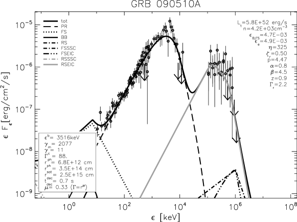
Figure 1.— GRB 090510 fit with a magnetic model ($\chi^{2}/$dof=107.6/97). In the upper figure lines represent the model. The points with the error bars can be thought of as measured values, though they are themselves model dependent (i.e. for different models they are not the same). They are calculated from the model convolved with the detectors’ responses (step curve on lower figure) and their relation to the observed counts (crosses on lower figure). For brevity we do not show the plot with the convolved spectra for other bursts.

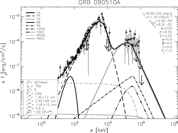
Figure 2.— GRB 090510 fit with a baryonic model ($\chi^{2}/$dof=107.1/97). Other notations are the same as Fig. 1

4.2. GRB 080916C fit for time integrated spectrum

GRB 080916C is one of the most intensive bursts ever detected (Abdo & the Fermi Collaboration, 2009). Its spectrum is consistent with the Band function throughout the Fermi energy range and in all the analyzed intervals (though there was weak evidence of an extra component (Abdo & the Fermi Collaboration, 2009)). The extremal magnetic and baryonic fits are shown in Fig. 3.

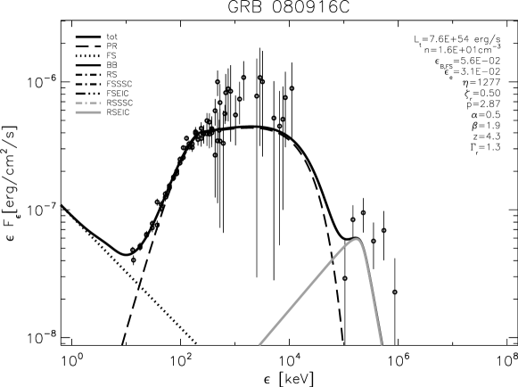
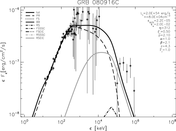
Figure 3.— Fit for GRB 080916C, for the entire interval, with a magnetic model (above, $\chi^{2}=113.6$, d.o.f.=$98$) and baryonic model (below, $\chi^{2}=129.7$, d.o.f.=$98$). The figures show the models and the data points obtained by scaling the measured count rates with respect to the convolved models.

4.3. GRB 090926A fit for the time resolved spectrum

Ackermann & the Fermi collaboration (2011) fitted the spectrum of this burst with a Band function and an extra power-law with a high energy cutoff. Using data from Zhang et al. (2011) the whole interval of the burst cannot be well fit with a simple analytical model, suggesting strong spectral evolution. We thus use the time resolved data for this GRB. We divided the burst in 4 intervals (with limits at 0, 4, 7, 11.5 and 19 s with respect to the trigger time). The first interval has no GeV range emission, and we drop it from our analysis.

We found that both the magnetic and the baryonic photosphere model can give an accurate description of the resolved data (see Fig. 4 for a superposition of magnetic and baryonic models and the models and data for the first interval on Fig. 5 ).

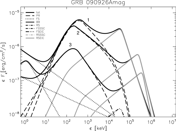
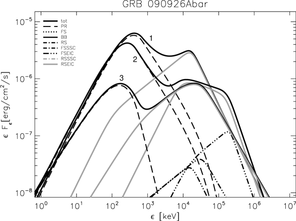
Figure 4.— GRB 090926A with three intervals fitted using the magnetic (top) and baryonic (bottom) photosphere model. We have displayed only a small number of components. The numbers indicate the intervals: 1: 4-7 s, 2: 7-11 and 3: 11.5-19 s. The 0-4 s period could not be fitted, because no LAT photons were detected.

Reduced $\chi^{2}_{r}$ values are in the range $1.4-1.8$ for the magnetic model, and $1.2-2.5$ in the baryonic case. Generally, $\epsilon_{e}$, $\epsilon_{B}$ and terminal Lorentz factors ($\eta$) are systematically lower in the baryonic case, the external density is systematically higher, while the other parameters are roughly in the same range for both cases. We note as a general trend, the magnetic model yielded better fits for the data.

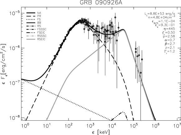
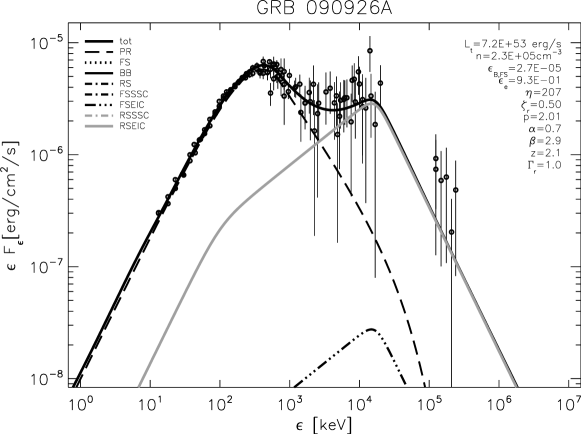
Figure 5.— Examples of magnetic (above, $\chi^{2}=182.9$, d.o.f.=$115$) and baryonic (below, $\chi^{2}=184.5$, d.o.f.=$115$) models with the data overplotted for GRB 090926A’s 4-7 s interval (see also Fig. 4).

4.4. GRB 090902B fit for the time resolved spectra

GRB 090902B (Abdo & the Fermi collaboration, 2009) has a relatively sharp Band spectrum with an underlying power law component. While a simple Planck function is too narrow to fit the spectrum, a multicolor blackbody and an underlying power law can fit the data equally well (Ryde et al., 2010). The fit for the entire duration of the burst did not give an acceptable fit for neither of the models, possibly due to the strong spectral evolution. It has been shown that this burst involves a strong spectral evolution (e.g. Zhang et al., 2011)

In order to account for spectral evolution, we have defined $10$ intervals bracketed by the $0,5,7.3,9.7,12,14.3,16.7,19,21.3,23.7$ and $26$ s marks relative to trigger (see Fig. 6).

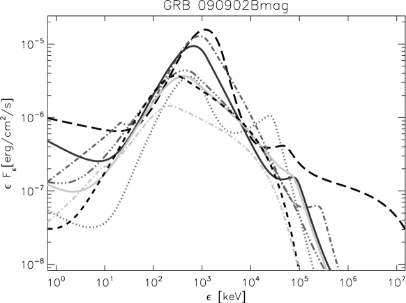
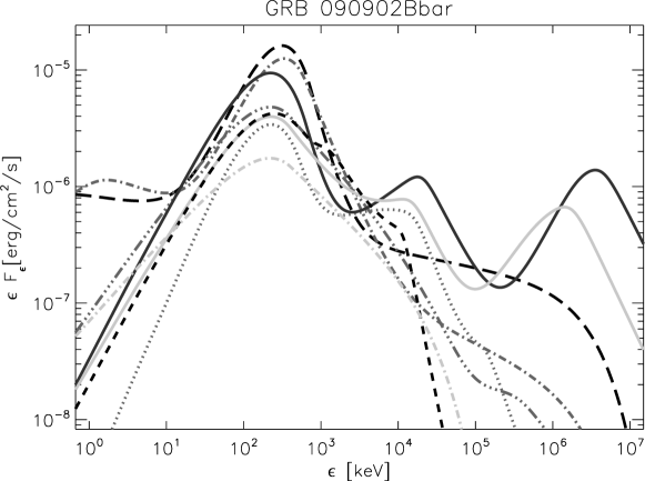
Figure 6.— GRB 090902B magnetic models (upper) and baryonic (lower). The time intervals depicted: 0-5 s: gray-dotted, 7.3-9.7 s: black-long dashed, 9.7-12 s: gray-dash-dotted, 12-14.3 s: gray-dash-dot-dot-dot, 14.3-16.7 s: black-continuous, 16.7-19 s: gray-continuous, 19-21.3 s: black-dashed, 21.3-23.7 s: light gray-dash-dotted.

$\epsilon_{e}$ varies in the range $\approx 0.001-0.7$, and it is similar for both models. The terminal Lorentz factor is systematically higher in the magnetic case and it is above $400$ in all intervals, while in the baryonic case, it is below $250$. The external density, is systematically lower in the magnetic case, while the magnetic parameter at the deceleration radius and the semirelativistic shocks’ Lorentz factor in the photosphere are systematically higher in the magnetic case. These parameters are all within the normal ranges found previously from fitting afterglow and prompt emission data on a wider sample of bursts. Here, we do not find any obvious trend for an evolution of the parameters throughout this burst. For an example fit for this burst’s first interval, see Fig. 7.

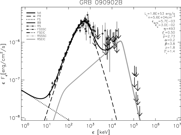
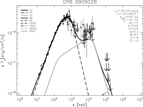
Figure 7.— Examples of magnetic (above, $\chi^{2}=102.3$, d.o.f.=$92$) and baryonic (below, $\chi^{2}=96.7$, d.o.f.=$92$) models with the data overplotted for GRB 090909B’s 0-5 s interval (see also Fig. 6 - gray-dotted curve).

5. Discussion

Possible relation between $\mu$ and observed trends.- In our fits we have purposefully avoided introducing any of the observed phenomenological correlations claimed for GRBs, since these have errors and biases which require extensive consideration and would complicate the analysis. However, it is interesting to speculate on the possible values of $\mu$ in the context of some of these phenomenological correlations.

In the $\eta>\eta_{T}$ case it seems simple considerations do not yield a consistent value for $\mu$, and this needs to be examined further. In the other case ($\eta<\eta_{T}$), there is no $\mu$ dependence, but we only need to assume one of the relations to obtain approximately the other one; e.g. if we assume $\eta\propto L^{0.3}$ (Lü et al., 2012), we get $\varepsilon_{b}\propto L^{0.4}$, fairly close to the Yonetoku relation.

Although we did not find any cases where the main MeV episode was provided by the thermal component, such cases have been discussed based based on more elaborate radiation transfer models, e.g. by Pe’er & Ryde (2011); Beloborodov (2012); Vurm et al. (2012) and others, typically for baryonic dynamics. In our simplified treatment the thermal component was taken as a simple blackbody function, instead of a broader multicolor blackbody as in, e.g. (Ryde et al., 2010). Such multicolor fits including our other variables would be much more cumbersome, but in principle, if we make a quick calculation similar to that in the previous paragraph, using Eq. 13 instead of Eq. 10, this would imply $\mu\approx 0.5$.

It is interesting to note that for the magnetically dominated model ($\eta>\eta_{T}$ and $\mu=1/3$), the peak energy does not depend on either the luminosity and the terminal Lorentz factor, and has a value of $\sim 300\hbox{~{}keV}$, corresponding to the clustering, observed by e.g. BATSE (Kaneko et al., 2006). There is a weak dependence on $r_{0}$ and redshift.

Comparison of the baryonic photosphere model with the magnetic model.- The main difference between the magnetic and the baryonic model in terms of the physical parameters involved in the GRBs is the initial dependence of the Lorentz factor on the radius (see equ. 1).

The main manifestation of this difference in terms of the observed spectrum is the strength of the thermal component from the photosphere. Because of the different dynamics, the magnetic model results in a sub-dominant thermal component, while in the case of the baryonic dynamics the black body component can have a more prominent contribution.

The main goal of this article has been to present a generalized formalism for models with an arbitrary acceleration of the GRB ejecta, valid for magnetic and baryonic dynamics. By means of an analysis of the brightest bursts, and properly accounting for the instrumental effects, we have shown that both an extremal magnetic and a baryonic model can provide adequate fits to the spectrum. Although in some of the cases the magnetic model provides a marginally better fit to the data, the difference is not significant enough to decide in favor of either extremal model.

Constraints on the parameters.- As we can see from Table 1. we can constrain some of the physical parameters of the models, except for the magnetic parameter at the deceleration radius, and in some cases the interstellar density is also difficult to constrain.

We found that the burst spectra are consistent with both the magnetic and the baryonic models presented here. A possible discrimination would require further theoretical considerations, or else other observational considerations; e.g. the length of the deceleration time should be the same order as the observed delay of the GeV emission. Another discriminant would be how well a model can reproduce the observed correlations between the rest-frame peak energy and e.g. luminosity would. As we indicated above, the extreme magnetic photosphere model appears to be better in accommodating these constraints.

One of the main differences between the two models is the systematically higher value of the coasting Lorentz factor (LF) in the magnetic model. This can be understood as follows: by applying two models to the same data the photospheric LF is the best constrained by the observations. While in the baryonic case this is just the terminal LF, in the magnetic case the ejecta is still accelerating at the photosphere, having a larger coasting LF.

In GRB 090510 Abdo et al. (2009) noted a correlation between the keV range radiation and the GeV radiation (but no correlation with the MeV radiation). Based on their spectrum, the additional power-law would be the responsible for explaining this correlation. In the framework of this generalized photospheric model, such a correlation can be explained if these two components have a common source: e.g. the keV emission is ascribed to the forward shock (FS) synchrotron and the GeV to the forward shock synchrotron-self Compton (FS-SSC); or if a reverse shock is present (as proposed in this work), the keV radiation can be due to the reverse shock synchrotron-self Compton (RS-SSC) and the GeV is produced by the reverse shock external inverse Compton (RS-EIC).

Conclusions.- In summary, we have shown that a simple dissipative photosphere model of the prompt emission of GRB based on synchrotron radiation can fit well the joint Fermi GBM and LAT data for the four brightest bursts with sufficiently detailed information. We have introduced a general formalism for treating the jet acceleration dynamics ranging between an extreme magnetically dominated to a baryon dominated dynamics regime. Both types of dynamics give acceptable fits to the data on these four bursts. Additional considerations involving statistical trends over a much larger sample of bursts might favor slightly the magnetic models, but firm conclusions would require detailed fits over much larger samples than undertaken here.

We acknowledge partial support from NASA NNX09AL40G and OTKA K077795 (PV, PM) and NASA SAO SV4-74018 and NASA SAO GO1-12102X (BBZ). We thank Kazumi Kashiyama, Yi-Zhong Fan and the anonymous referee for comments and suggestions.

References

- Abdo & the Fermi Collaboration (2009) Abdo, A., & the Fermi Collaboration. 2009, Science, 0036, 8075
- Abdo et al. (2009) Abdo, A. A. et al. 2009, Nature, 462, 331
- Abdo & the Fermi collaboration (2009) Abdo, A. A., & the Fermi collaboration. 2009, ApJ, 706, L138, 0909.2470