The $\delta N$ formula is the dynamical renormalization group

Abstract

We derive the ‘separate universe’ method for the inflationary bispectrum, beginning directly from a field-theory calculation. We work to tree-level in quantum effects but to all orders in the slow-roll expansion, with masses accommodated perturbatively. Our method provides a systematic basis to account for novel sources of time-dependence in inflationary correlation functions, and has immediate applications. First, we use our result to obtain the correct matching prescription between the ‘quantum’ and ‘classical’ parts of the separate universe computation. Second, we elaborate on the application of this method in situations where its validity is not clear. As a by-product of our calculation we give the leading slow-roll corrections to the three-point function of field fluctuations on spatially flat hypersurfaces in a canonical, multiple-field model.

1 Introduction

Since Maldacena’s computation of the three-point function produced by an epoch of single-field inflation [1], considerable effort has been invested in obtaining correlation functions for more complex scenarios. In part this investment has been motivated by the increasing sophistication of observational cosmology. But an equally important influence has been the drive to understand the implications of our inflationary theories, especially in examples with many interacting degrees of freedom.

The tool used to extract predictions from inflationary scenarios is quantum field theory, in which each observable is constructed from correlation functions. Quantum field theory incorporates the effect of fluctuations on all scales, making each correlation function potentially sensitive to both short- and long-distance effects. Over very short distances this implies that they must be defined carefully by a renormalization prescription, as in flat spacetime. But the most interesting outcome of our investment in studying correlation functions has been the realization that they have a rich infrared structure which is very different to the case of flat spacetime. Some aspects of this structure were reviewed in Refs. [2, 3, 4].

Nontrivial structure in correlation functions is often associated with the existence of kinematic hierarchies. A paradigmatic example from particle physics is a hadronic jet carrying some large energy $E$ but small invariant mass $m_{\text{jet}}$. Another is electroweak processes at large momentum transfer $s\gg M_{Z}^{2}$. (Here $s$ is the Mandelstam variable and $M_{Z}$ is the mass of the $Z$ boson.) The kinematic region where ratios such as $E/m_{\text{jet}}$ or $s/M_{Z}^{2}$ become large is called the Sudakov region. In this region logarithms of large ratios invalidate perturbation theory, and to obtain even a qualitative description requires resummation.

Analogues of these effects are responsible for the rich infrared structure of inflationary correlation functions. Viewed as a sum of Feynman diagrams, a generic $n$-point function is characterized by the comoving momenta carried by each propagator. At tree-level these are linear combinations $\bm{\mathrm{{q}}}_{i}$ of the external momenta $\{\bm{\mathrm{{k}}}_{1},\ldots,\bm{\mathrm{{k}}}_{n}\}$. Another scale is the comoving Hubble length $\tau\sim(aH)^{-1}$ where $a$ is the scale factor and $H=\dot{a}/a$ is the Hubble rate. Sudakov-like logarithms involving ratios of these scales appear in each correlation function.

When there are no hierarchies among the $|\bm{\mathrm{{q}}}_{i}|$ and $\tau$, each of these scales will be comparable to some reference scale $k_{\ast}$. If the $n$-point functions are expressed in terms of background quantities evaluated at the horizon-crossing time for $k_{\ast}$, the Sudakov-like logarithms are small and the correlation functions are simple. However, if large hierarchies exist it will not be possible to find a $k_{\ast}$ for which all logarithms are small and the correlation functions develop a complex structure. Indeed, we will see that it is necessary to carry out a resummation, just as for hadronic jets and high-energy electroweak observables. Understanding the details of this enhanced structure is particularly important because correlation functions with large hierarchies are valuable observables: for example, $n$-point functions with $q_{i}/q_{j}\gg 1$ can be used to determine nonlinear and stochastic halo bias [7]. But despite their significance, a systematic treatment of these effects has not appeared in the literature.

In this paper we begin a systematic treatment of correlation functions containing Sudakov-like logarithms. We focus on logarithms containing the comoving Hubble scale $\tau$, which may all be rewritten in the form $\ln|k_{\ast}\tau|$ (perhaps at the cost of introducing other logarithms of the form $\ln q_{i}/k_{\ast}$). In this form they coincide with the ‘time-dependent’ logarithms $\ln|k_{\ast}\tau|$ described in Ref. [2]; see also Ref. [4]. We will return to the remaining ‘scale’ and ‘shape’ logarithms (involving $\ln q_{i}/k_{\ast}$ and $\ln q_{i}/q_{j}$, respectively [8]) in a future publication. We work to tree-level in quantum effects but to all orders in the slow-roll expansion. In particular, this means that masses are accommodated perturbatively. We will comment on the implications of this choice as we develop our argument in §§3–5 below.

Separate-universe formulae.

It has been understood for some time that logarithms of the form $\ln|k_{\ast}\tau|$ describe time evolution of each $n$-point function [9, 10, 11, 12]. But, although the necessity to account for time evolution is well-known, the precise role of the $\ln|k_{\ast}\tau|$ terms has received comparatively little attention. Most discussion of time dependence are framed in terms of the ‘separate universe’ approach to perturbation theory [13, 14, 15, 16]. On very large scales this gives a description of a perturbed universe by patching together unperturbed solutions with different initial conditions. One implementation follows Sasaki & Tanaka [17], who argued that the superhorizon limit of perturbation theory could be obtained from Jacobi fields of the background phase space. (A similar interpretation was recently given in Ref.[18].) Related discussions of perturbation theory on large scales were given in Refs. [19, 20, 21]. On the basis of these arguments one can determine the evolution of correlation functions by tracking the evolution of these Jacobi fields and averaging over a suitable ensemble of stochastic initial conditions.

This approach gives a reliable description of effects occurring on superhorizon scales, but it cannot describe subhorizon physics or phenomena which occur near the epoch of horizon exit. For example, this leads to some ambiguity about the precise ensemble of initial conditions which should be used when computing correlation functions, to which we will return in §5.1. In this paper we argue that the separate-universe method can be reproduced by resummation of Sudakov-like logarithms. Among other benefits, this provides precise information about the role of horizon-crossing effects which cannot be captured from the superhorizon limit of perturbation theory.

After constructing suitable Jacobi fields and setting up an ensemble of initial conditions $\delta\phi_{i}(\bm{\mathrm{{k}}}_{1})$, the separate-universe approach we have just described asserts that the two- and three-point functions for a set of light scalar fields during inflation satisfy [16]

$$\langle\delta\phi_{\alpha}(\bm{\mathrm{{k}}}_{1})\delta\phi_{\beta}(\bm{\mathrm{{k}}}_{2})\rangle \supseteq\frac{\partial\phi_{\alpha}}{\partial\phi_{i}^{\ast}}\frac{\partial\phi_{\beta}}{\partial\phi_{j}^{\ast}}\langle\delta\phi_{i}(\bm{\mathrm{{k}}}_{1})\delta\phi_{j}(\bm{\mathrm{{k}}}_{2})\rangle_{\ast}$$ (1.1a)

$$\langle\delta\phi_{\alpha}(\bm{\mathrm{{k}}}_{1})\delta\phi_{\beta}(\bm{\mathrm{{k}}}_{2})\delta\phi_{\gamma}(\bm{\mathrm{{k}}}_{3})\rangle \supseteq\frac{\partial\phi_{\alpha}}{\partial\phi_{i}^{\ast}}\frac{\partial\phi_{\beta}}{\partial\phi_{j}^{\ast}}\frac{\partial\phi_{\gamma}}{\partial\phi_{k}^{\ast}}\langle\delta\phi_{i}(\bm{\mathrm{{k}}}_{1})\delta\phi_{j}(\bm{\mathrm{{k}}}_{2})\delta\phi_{k}(\bm{\mathrm{{k}}}_{3})\rangle_{\ast}$$

$$\quad\mbox{}+\frac{\partial^{2}\phi_{\alpha}}{\partial\phi_{i}^{\ast}\partial\phi_{j}^{\ast}}\frac{\partial\phi_{\beta}}{\partial\phi_{k}^{\ast}}\frac{\partial\phi_{\gamma}}{\partial\phi_{m}^{\ast}}\int\frac{\mathrm{d}^{3}q}{(2\pi)^{3}}\;\langle\delta\phi_{i}(\bm{\mathrm{{k}}}_{1}-\bm{\mathrm{{q}}})\delta\phi_{k}(\bm{\mathrm{{k}}}_{2})\rangle_{\ast}\langle\delta\phi_{j}(\bm{\mathrm{{q}}})\delta\phi_{m}(\bm{\mathrm{{k}}}_{3})\rangle_{\ast}$$

$$\quad\mbox{}+\text{cyclic permutations}.$$ (1.1b)

We have adopted the notation of Refs. [18, 22], which will be used throughout this paper. On the left-hand side, each correlation function is evaluated at some late time $t$ and transforms as a tensor in the tangent space associated with the field-space coordinate $\phi_{\alpha}(t)$. Indices in this tangent space are labelled $\{\alpha,\beta,\ldots\}$. On the right-hand side each correlation function is evaluated at the horizon-crossing time $t_{\ast}$ for the reference scale $k_{\ast}$, and transforms as a tensor in the tangent space associated with the field-space coordinate $\phi_{i}(t_{\ast})$. Indices in this tangent space are labelled $\{i,j,\ldots\}$. Where the field-space manifold is curved it is essential to preserve this distinction [22]. In this paper we will work with a flat field-space metric except in §5.2 but this index convention remains convenient. The bitensors $\partial\phi_{\alpha}/\partial\phi^{\ast}_{i}$, $\partial^{2}\phi_{\alpha}/\partial\phi^{\ast}_{i}\partial\phi^{\ast}_{j}$ measure variation of the inflationary trajectory under a change of initial conditions at the horizon-crossing time for the reference scale, and the symbol ‘$\supseteq$’ indicates that subleading corrections from ‘loop’ diagrams have been ignored together with disconnected contributions.

Eqs. (1.1a)–(1.1b) make a number of strong assertions. First, Eq. (1.1a) asserts that, at all times and accounting for large contributions from all orders in the slow-roll expansion, the two-point function can be written as a linear combination of its values at some arbitrary earlier time with coefficients $\partial\phi_{\alpha}/\partial\phi_{i}^{\ast}$. This implies that (at least when decaying modes have become negligible) all time-dependent Sudakov-like logarithms can be factorized into these coefficients. Here and below, ‘to all orders in the slow-roll expansion’ is a statement about a perturbative expansion in terms of slow-roll parameters evaluated at the horizon-crossing time for $k_{\ast}$.

Second, Eq. (1.1b) asserts that any time-dependent Sudakov-like logarithms appearing in the three-point function exhibit a similar factorizable structure. In principle the three-point function could have arbitrary dependence on the external momenta $k_{i}$ [1, 23]. Therefore, at each order, the Sudakov-like logarithms could enter with different functions of the $k_{i}$. But Eq. (1.1b) asserts that, to all orders in the slow-roll expansion, almost all Sudakov-like logarithms factorize into the coefficients $\partial\phi_{\alpha}/\partial\phi_{i}^{\ast}$ which appear in the two-point function (1.1a). Exceptions are allowed only for Sudakov-like logarithms which multiply functions of the $k_{i}$ obtainable from a product of two-point functions. For massless fields, or where masses are taken into account perturbatively, these are the ‘local’ momentum combinations $(k_{2}^{3}k_{3}^{3})^{-1}$ and its permutations. Even for these exceptions, Eq. (1.1b) requires that the resummation of Sudakov-like logarithms produces a result which is related in a nontrivial way to the factorizable coefficients already present in the two-point function.

Each of these assertions is a complex statement, applicable to all orders in the slow-roll expansion, about the structure of infrared divergences which can be produced by the underlying quantum field theory. Although these results are implied by the perturbation-theory results described above, it is nontrivial to see how they are reproduced by the Sudakov-like logarithms which arise from the underlying quantum field theory. In this paper we explain how this occurs by deducing the time-dependent structure of each correlation function directly from the Sudakov-like divergences it contains. We will see that this provides a practical and convenient means to compute the evolution of each $n$-point function in cases where the separate universe picture is complicated to apply, or an untrustworthy guide for our intuition.

Summary.

The Sudakov-like time-dependent logarithms in inflationary correlation functions are qualitatively similar to those occurring in particle physics, and therefore can be understood using the same tools. In §2 we sketch the main steps, focusing on a physical interpretation of the ‘factorizable’ structure. In §3 we begin to develop this argument in detail. The strategy breaks into two parts.

• First, in §4.2 we prove a factorization theorem which provides constraints on the terms in each correlation function which can be logarithmically enhanced. This factorization theorem plays the same role as a proof of renormalizability in applying renormalization-group arguments to the ultraviolet behaviour of correlation functions: it guarantees that all large logarithms can be assembled into a finite number of ‘renormalized’ functions.

• Second, in §4.3, we derive a renormalization group equation (‘rge’) which can be used to determine these unknown ‘renormalized’ functions. Once the renormalization group equations have been solved the full correlation function can be reconstructed. It will turn out that the rges are equivalent to the transport equations used to determine $\partial\phi_{\alpha}/\partial\phi_{i}^{\ast}$ and their higher derivatives [24, 25, 26, 27, 28, 18, 22].

In §5 we illustrate our method using examples. When justified from the superhorizon limit of perturbation theory the separate-universe approach requires a set of initial conditions, usually assumed to be generated from quantum fluctuations which become classical after passing outside the horizon. Implicit in this point of view is a ‘matching’ between quantum and classical calculations. Several authors have noted that the precise choice of matching time is ambigious, which could lead to uncertainties in an accurate calculation [29, 30, 31]. In §5.1 we revisit this question using the rge approach, in which there is no need to invoke a matching from quantum to classical evolution because the entire calculation takes place within the framework of quantum field theory. We show how this gives a unique prescription which resolves the matching ambiguity.

In §5.2 we illustrate the practical utility of the rge method by using it to determine evolution equations for covariant versions of the coefficients $\partial\phi_{\alpha}/\partial\phi_{i}^{\ast}$ and their higher-order generalizations in the presence of a nontrivial field-space metric. These coefficients are not straightforward to determine using classical intuition, making the renormalization-group approach simple and reliable. This example could be adapted to more complex cases, perhaps including the effect of loop corrections, where the usual classical separate-universe arguments do not function or are prohibitively difficult to apply.

In §6 we conclude with a short discussion of our main results. We provide details of the next-order calculation of the three-point correlation function (which is required to deduce an appropriate renormalization group equation for the coefficient functions) in Appendix A.

Notation and conventions.

Throughout this paper, we adopt units in which $c=\hbar=1$. Our index conventions for scalar fields are described below Eqs. (1.1a)–(1.1b). We work with the action

$$S=\frac{1}{2}\int\mathrm{d}^{4}x\;\sqrt{-g}\,\Big{\{}M_{\mathrm{P}}^{2}R-\partial_{a}\phi_{\alpha}\partial^{a}\phi_{\alpha}-2V\Big{\}},$$ (1.2)

where $V=V(\phi)$ is an arbitrary potential and Latin indices $a$, $b$, …, are Lorentz indices contracted with the spacetime metric $g_{ab}$. Except where explicitly indicated, scalar field indices are contracted using the flat field-space metric $\delta_{\alpha\beta}$. We will generally set the reduced Planck mass $M_{\mathrm{P}}\equiv(8\pi G)^{-1/2}$ to unity.

2 Why is resummation necessary?

It is not at all clear from inspection of Eqs. (1.1a)–(1.1b) that they involve a resummation of time-dependent Sudakov-like logarithms. In this section and the next we explain why resummation is necessary and develop a heuristic approach to these equations. In §4 we will consider the same problem from a more formal viewpoint, that of the dynamical renormalization group.

To quadratic order, the action for fluctuations of the scalar fields $\phi_{\alpha}$ in (1.2), measured on uniform-expansion hypersurfaces, can be written

$$S=\frac{1}{2}\int\mathrm{d}^{3}x\,\mathrm{d}t\;a^{3}\left(\delta\dot{\phi}_{\alpha}\delta\dot{\phi}_{\alpha}-\frac{1}{a^{2}}\partial_{i}\delta\phi_{\alpha}\partial_{i}\delta\phi_{\alpha}-m_{\alpha\beta}\delta\phi_{\alpha}\delta\phi_{\beta}\right),$$ (2.1)

where an overdot denotes differentiation with respect to cosmic time. The mass-mixing matrix $m_{\alpha\beta}$ can be written explicitly in terms of slow-roll parameters [32, 33, 15]

$$m_{\alpha\beta}=V_{\alpha\beta}-\frac{1}{a^{3}}\frac{\mathrm{d}}{\mathrm{d}t}\left(\frac{a^{3}}{H}\dot{\phi}_{\alpha}\dot{\phi}_{\beta}\right)=V_{\alpha\beta}-3\dot{\phi}_{\alpha}\dot{\phi}_{\beta}-\varepsilon\dot{\phi}_{\alpha}\dot{\phi}_{\beta}-\frac{2}{H}\dot{\phi}_{(\alpha}\ddot{\phi}_{\beta)},$$ (2.2)

where $\varepsilon=-\dot{H}/H^{2}$ is the usual slow-roll parameter. Inflation occurs whenever $\varepsilon<1$. At lowest order in slow-roll the mass-matrix can be related to the ‘expansion tensor’ $u_{\alpha\beta}$ introduced in Ref. [18],

$$u_{\alpha\beta}=-\frac{m_{\alpha\beta}}{3H^{2}}.$$ (2.3)

Two-point function.

It is convenient to work in conformal time, defined by $\tau=\int^{t}_{\infty}\mathrm{d}t^{\prime}/a(t^{\prime})$. For the two-point function only a single hierarchy can be generated, measured by the ratio of $k$ to the comoving Hubble scale $aH\approx-\tau^{-1}$. Therefore $|k\tau|\approx 1$ at horizon crossing. Working to next-order in the slow-roll expansion and evaluating the two-point function at least a little after horizon-crossing we find

$$\begin{split}\langle\delta&\phi_{\alpha}(\bm{\mathrm{{k}}}_{1})\delta\phi_{\beta}(\bm{\mathrm{{k}}}_{2})\rangle_{\tau}=(2\pi)^{3}\delta(\bm{\mathrm{{k}}}_{1}+\bm{\mathrm{{k}}}_{2})\frac{H_{\ast}^{2}}{2k^{3}}\\ &\times\left\{\delta_{\alpha\beta}\left[1+2\varepsilon_{\ast}\left(1-\gamma_{\mathrm{E}}-\ln\frac{2k}{k_{\ast}}\right)\right]+2u_{\alpha\beta}^{\ast}\left[2-\gamma_{\mathrm{E}}-\ln(-k_{\ast}\tau)-\ln\frac{2k}{k_{\ast}}\right]+\cdots\right\},\end{split}$$ (2.4)

where ‘$\cdots$’ indicates higher-order corrections which we have not computed. We have set $k=k_{1}=k_{2}$ to be the common magnitude of the external momenta and dropped contributions which decay like positive powers of $\tau$. The scale $k_{\ast}$ determines a horizon-crossing time around which we have chosen to Taylor-expand background time-dependent quantities such as $H$. Evaluation at the horizon-crossing time for $k_{\ast}$ is denoted by a subscript ‘$\ast$’. At this stage its precise assigment is arbitrary and can be chosen to suit our own convenience. The terms involving $\ln k/k_{\ast}$ and $\ln(-k_{\ast}\tau)$ are our first examples of Sudakov-like logarithms.

This result has appeared in various forms in the literature. It was given in the single-field case by Stewart & Lyth [34], who worked directly in terms of the conserved comoving-gauge curvature perturbation $\mathcal{R}$. The corresponding result for field fluctuations in the uniform-expansion gauge was given by Nakamura & Stewart [35], who accounted for multiple fields and a nontrivial field-space metric. Higher-order corrections were given by Gong & Stewart, who developed an algorithmic approach to compute them using Green’s functions of the Mukhanov–Sasaki equation [36, 37].

Callan–Symanzik equation.

The reference scale $k_{\ast}$ is not physical, and therefore the correlation functions cannot depend on it. Invariance under a change in $k_{\ast}$ is expressed by the Callan–Symanzik equation. Taking all background quantities to be functions of the fields $\phi_{\alpha}$, this equation can be written

$$\left(\frac{\partial}{\partial\ln k_{\ast}}+\frac{\partial\phi_{\lambda}^{\ast}}{\partial\ln k_{\ast}}\frac{\partial}{\partial\phi_{\lambda}^{\ast}}\right)\langle\delta\phi_{\alpha_{1}}(\bm{\mathrm{{k}}}_{1})\cdots\delta\phi_{\alpha_{n}}(\bm{\mathrm{{k}}}_{n})\rangle=0.$$ (2.5)

The differential operator in brackets $(\cdots)$ is simply the total derivative $\mathrm{d}/\mathrm{d}\ln k_{\ast}$. Specializing (2.5) to the two-point function yields, to lowest-order in a slow-roll expansion,

$$\frac{\mathrm{d}\ln H_{\ast}}{\mathrm{d}\ln k_{\ast}}+\varepsilon_{\ast}=0.$$ (2.6)

As above, a subscript ‘$\ast$’ indicates evaluation at the horizon-crossing point for $k_{\ast}$. Since (2.6) holds for any $k_{\ast}$ it expresses the condition $\varepsilon=-\dot{H}/H^{2}$ which is satisfied for any change of the background fields $\phi_{\alpha}$ which themselves satisfy the background equations of motion. This is sometimes expressed by saying that the change should be ‘on-shell’. Eq. (2.6) guarantees that we are free to change $k_{\ast}$ provided that we compensate by adjusting all background quantities according to their classical equations of motion. The appearance of classical equations is a consequence of our restriction to tree-level processes.

Time evolution.

We now return to Eq. (2.4) and consider its behaviour for different values of $k$ and $\tau$.

An expression such as (2.4) is said to be computed using fixed order perturbation theory, because the calculation is carried to a predetermined order in the slow-roll expansion. When $k$ is comparable to $aH$, Eq. (2.6) shows that we can choose $k_{\ast}$ to be approximately their common magnitude provided we evaluate background quantities near the horizon-crossing time for $k$. Then $\ln(-k_{\ast}\tau)$ and $\ln k/k_{\ast}$ will both be negligible, and a fixed-order expression such as Eq. (2.4) is a good approximation. It is dominated by its lowest-order term $H_{\ast}^{2}/2k^{3}$.

More than a few e-folds after horizon-crossing the hierarchy $k/aH=|k\tau|$ becomes exponentially small. No matter how we choose $k_{\ast}$ it is no longer possible to make both $\ln k/k_{\ast}$ and $\ln(-k_{\ast}\tau)$ negligible. Therefore we must accept the appearance of large, growing contributions which cannot be absorbed into background quantities by a choice of evaluation time. Growing terms of this kind are potentially hazardous. They are sometimes described as divergences, because on its own $\ln(-k_{\ast}\tau)$ becomes unboundedly large as $\tau\rightarrow 0$. This is simply an artefact of perturbation theory, in the same way that the Taylor expansion of any function

$$f(x)=f(x_{0})+f^{\prime}(x_{0})(x-x_{0})+\cdots$$

appears to diverge when $|x-x_{0}|\gg 1$. In reality, when $\varepsilon_{\ast}\ln(-k_{\ast}\tau)\sim 1$ we must sum an infinite number of terms from a fixed-order expression such as (1.1a) before we can determine even its qualitative behaviour. Therefore, unless some principle or symmetry enforces a precise cancellation, fixed-order perturbation theory can never provide an adequate description. This obligation to deal with an infinite sequence of terms of the form $[\varepsilon_{\ast}\ln(-k_{\ast}\tau)]^{n}$ was emphasized by Weinberg [41], who went on to speculate that the methods of the renormalization group could be used to perform the resummation, in analogy with the case of Sudakov effects in QCD. In this paper we show that this is indeed the case.

We conclude that any expression which is valid to arbitrarily late times, such as (1.1a), must resum an infinite number of terms. For example, consider the well-studied model of double quadratic inflation [42, 29, 43, 44]. The action is

$$S=-\dfrac{1}{2}\int\mathrm{d}^{4}x\;\sqrt{-g}\,\Big{\{}R+\partial_{a}\varphi\partial^{a}\varphi+\partial_{a}\chi\partial^{a}\chi+m_{\varphi}^{2}\varphi^{2}+m_{\chi}^{2}\chi^{2}\Big{\}},$$ (2.7)

where $\varphi$ and $\chi$ are two light scalar fields with $m_{\varphi}$, $m_{\chi}<H$. We focus on the dimensionless two-point function $\Sigma_{\alpha\beta}$, defined by

$$\langle\delta\phi_{\alpha}(\bm{\mathrm{{k}}}_{1})\delta\phi_{\beta}(\bm{\mathrm{{k}}}_{2})\rangle_{\tau}=(2\pi)^{3}\delta(\bm{\mathrm{{k}}}_{1}+\bm{\mathrm{{k}}}_{2})\frac{\Sigma_{\alpha\beta}}{2k^{3}},$$ (2.8)

but similar remarks apply to higher $n$-point functions.

In Fig. 1 we present a typical super-horizon evolution of $\Sigma_{\varphi\varphi}$ calculated using the formula (1.1a). There is a clearly defined peak in the vicinity of $N=-\ln(-k_{\ast}\tau)\simeq 20$, caused by a turn of the trajectory in field space [45], after which $\Sigma_{\varphi\varphi}$ asymptotes to a constant. Inflation is ongoing through the entire evolution, with $\varepsilon$ growing to a maximum value $\sim 0.26$ near the peak. Fig. 1 shows clearly that $\Sigma_{\alpha\beta}$ can exhibit very rapid evolution. The linear approximation involving $\varepsilon_{\ast}\ln(-k_{\ast}\tau)$ is already poor for $N\gtrsim 10$ and is totally incorrect (even qualitatively) for $N\gtrsim 20$. If the initial time had been chosen closer to the peak, the linear approximation could easily have been invalidated within $\lesssim 1$ e-fold.

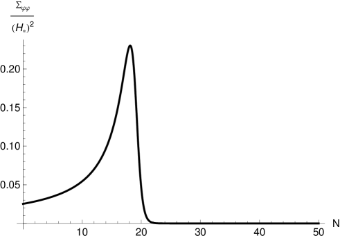
Figure 1: Super-horizon evolution of the two-point function $\Sigma_{\varphi\varphi}$ in the double-quadratic model (2.7), normalized by the Hubble scale at horizon crossing. This evolution is for the scale which left the horizon (at $N=0$) fifty e-folds before the end of inflation (at $N=50$). The initial conditions were $\varphi_{\text{init}}=8.2M_{\mathrm{P}}$ and $\chi_{\text{init}}=12.9M_{\mathrm{P}}$ with $m_{\varphi}/m_{\chi}=9$.

The flat asymptote for $N\gtrsim 20$ is associated with convergence to an ‘adiabatic limit’ in which the uniform-density gauge curvature perturbation $\zeta$ is conserved [46]. To describe this asymptotic plateau certainly requires resummation of an infinite number of powers of $N=-\ln(-k_{\ast}\tau)$. In any finite combination the highest power of $N$ must eventually dominate, leading to power-law growth at large $N$. It is only in an infinite sum that sufficiently many terms remain available at high-order to balance the growing contribution at low orders, enabling $\Sigma_{\varphi\varphi}$ to be constant at late times.

3 Towards a resummation prescription

We have identified growth of the logarithmic ‘divergence’ in (2.4) with the infrared region where $k/aH\ll 1$. It represents the cumulative effect of interactions which operate over very many Hubble times. We would like to separate the physics of these interactions from the creation of fluctuations in each $k$-mode, which takes place over only a few Hubble times. The disparity of these timescales implies that, when they are created, the fluctuations do not depend on details of the inflationary model in which they are embedded. It is the systematic separation of short-distance, model-independent ‘hard’ physics and long-distance, model-dependent ‘soft’ effects which produces the factorization in Eqs. (1.1a)–(1.1b).

In this section we illustrate how to perform and interpret factorization of the two-point function, and indicate how to extend the method to higher $n$-point functions.

3.1 Factorization of the two-point function

We work with the dimensionless two-point function $\Sigma_{\alpha\beta}$ defined in Eq. (2.8). The formula (2.4) includes terms at lowest-order in the slow-roll expansion and $\operatorname{O}(\varepsilon)$ corrections. We describe these, respectively, as ‘lowest-order’ (lo) and ‘next-lowest order’ (or next-order, nlo) terms. Working to nlo, we identify

$$\Sigma_{\alpha\beta}^{\text{{nlo}}}\supseteq H_{\ast}^{2}\left(\delta_{\alpha\beta}+2r_{\alpha\beta}^{\ast}-2u^{\ast}_{\alpha\beta}\ln(-k_{\ast}\tau)-2M^{\ast}_{\alpha\beta}\ln\frac{2k}{k_{\ast}}\right).$$ (3.1)

The constant matrices $r_{\alpha\beta}$ and $M_{\alpha\beta}$ are

$$r^{\ast}_{\alpha\beta} =\varepsilon_{\ast}\delta_{\alpha\beta}(1-\gamma_{\mathrm{E}})+u^{\ast}_{\alpha\beta}(2-\gamma_{\mathrm{E}})$$ (3.2a)

$$M^{\ast}_{\alpha\beta} =\varepsilon_{\ast}\delta_{\alpha\beta}+u^{\ast}_{\alpha\beta}.$$ (3.2b)

Heuristic treatment.

In what follows, we assume that $\Sigma_{\alpha\beta}$ contains at most powers of $\ln k$, but not powers of $k$ itself. This is a consequence of approximate scale invariance. Our aim is to separate the long- and short-distance contributions to (3.1). It was explained above that when $k/aH\ll 1$ we cannot make a choice of $k_{\ast}$ which eliminates all large logarithms. In effect, we do not have enough free scales to absorb every large contribution: it is only possible to use $k_{\ast}$ to eliminate contributions from one of $\ln k/k_{\ast}$ and $\ln(-k_{\ast}\tau)$. We choose $k_{\ast}=k$ to eliminate $\ln k/k_{\ast}$ and  introduce a new, arbitrary ‘factorization scale’ $k_{\text{{f}}}$. (However, we continue to denote quantities evaluated at the horizon-crossing time for $k_{\ast}$ with a subscript ‘$\ast$’.) Ultimately, we will see that the factorization scale describes the boundary between long- and short-distance physics. We write

$$\begin{split}\Sigma^{\text{{nlo}}}_{\alpha\beta}&\supseteq H_{\ast}^{2}\Big{(}\delta_{\alpha\beta}+2\tilde{r}^{\ast}_{\alpha\beta}-2u^{\ast}_{\alpha\beta}\Big{[}\ln\frac{k}{k_{\text{{f}}}}+\ln(-k_{\text{{f}}}\tau)\Big{]}\Big{)}\\ &=H_{\ast}^{2}\Big{(}\delta_{\alpha i}-u^{\ast}_{\alpha i}\ln(-k_{\text{{f}}}\tau)\Big{)}\Big{(}\delta_{\beta j}-u^{\ast}_{\beta j}\ln(-k_{\text{{f}}}\tau)\Big{)}\Big{(}\delta_{ij}+2\tilde{r}^{\ast}_{ij}-2u^{\ast}_{ij}\ln\frac{k}{k_{\text{{f}}}}\Big{)},\end{split}$$ (3.3)

where $\tilde{r}_{\alpha\beta}=r_{\alpha\beta}-M_{\alpha\beta}\ln 2$. In the first line $k_{\text{{f}}}$ cancels out. The second line is valid to next-order, which is the accuracy to which we are working. Based on the structure of (3.3), we introduce a ‘form-factor’ $\Gamma_{\alpha i}$, which is a function only of $\tau$ and the factorization scale $k_{\text{{f}}}$,

$$\Sigma_{\alpha\beta}=H_{\ast}^{2}\Gamma_{\alpha i}\Gamma_{\beta j}\Big{(}\delta_{ij}+2\tilde{r}^{\ast}_{ij}-2u^{\ast}_{ij}\ln\frac{k}{k_{\text{{f}}}}\Big{)}.$$ (3.4)

We will see that this form-factor modifies the lowest-order functional dependence of $\Sigma_{\alpha\beta}$ on background quantities, giving the two-point function an enhanced structure which is not visible in fixed-order perturbation theory. Modifications of this type are an inevitable consequence of large contributions which cannot be absorbed into a change of evaluation point for the background quantities already present in a fixed-order expression such as (2.4) or (3.1).

Since $\Sigma_{\alpha\beta}$ must be independent of $k_{\text{{f}}}$ it is possible to write a Callan–Symanzik equation similar to (2.5). For (3.4) to be independent of $k_{\text{{f}}}$ requires

$$\frac{\mathrm{d}\Gamma_{\alpha i}}{\mathrm{d}\ln k_{\text{{f}}}}=-\Gamma_{\alpha j}u_{ji}.$$ (3.5)

In Eqs. (3.3)–(3.5) we have made use of the index convention described in §1. The indices $\alpha$, $\beta$, … label the tangent space at the late time $\tau$, whereas indices $i$, $j$, … label the tangent space at the horizon-crossing time for the factorization scale $k_{\text{{f}}}$. Note that in (3.5) we have rewritten the time of evaluation for $u_{ij}$ as this horizon-crossing time. This is formally acceptable because the error we incur is $\operatorname{O}(\varepsilon^{2})$ and therefore below the precision to which we are working. In §4 below we will see how to give a more mathematically satisfactory formulation of this argument. In this section the discussion is not intended to be rigorous, but to highlight the physical meaning of factorization.

Eq. (3.5) is the ‘backwards’ evolution equation introduced by Yokoyama et al. [24, 25, 26] for the separate-universe coefficient $\partial\phi_{\alpha}/\partial\phi_{i}$. This discussion shows that it can equally be regarded as a kind of renormalization-group equation for the ‘Sudakov-like’ form-factor $\Gamma_{\alpha i}$. Its solution requires an initial condition. This can be deduced from (3.3), which gives $\Gamma_{\alpha i}=\delta_{\alpha i}$ when $|k_{\text{{f}}}\tau|\sim 1$. In combination with (3.5) the initial condition enables us to give a physical interpretation of the factorization procedure (see Fig. 2). Our starting point is a fixed-order expression such as (3.1).

Figure 2: Scales appearing in factorization of the two-point function. At late times $\tau\rightarrow 0$, generating a large hierarchy between the horizon size $k_{H}=-\tau^{-1}$ and the fixed comoving scale $k$. The floating scale $k_{\text{{f}}}$ acts as a boundary between the ‘hard’ (short-distance, $k/aH\gtrsim 1$) and ‘soft’ (long-distance, $k/aH\lesssim 1$) parts of the calculation. Beginning with $k_{\text{{f}}}=k_{H}$, all soft effects are included in the fixed-order part of the calculation. The ‘renormalization group equation’ (3.5) allows us to slide $k_{\text{{f}}}$ towards $k$, successively absorbing long-distance effects in the Sudakov-like form-factor $\Gamma_{\alpha i}$. Eventually, only ‘hard’ effects dominated by comoving momenta $\sim k$ are included in the fixed-order part of the calculation.

We begin with $|k_{\text{{f}}}\tau|\sim 1$. With this choice the form-factors $\Gamma_{\alpha i}=\delta_{\alpha i}$ are trivial and contain no information, whereas the fixed-order piece involving $\ln k/k_{\text{{f}}}$ accounts for contributions from both long- and short-distance effects. These are effects arising from the regions $k/aH\gtrsim 1$ and $k/aH\lesssim 1$, respectively. We now use (3.5) to systematically move $k_{\text{{f}}}$ closer to $k$. This adjustment moves all effects generated up to the point where $k_{\text{{f}}}/aH\lesssim 1$ into $\Gamma_{\alpha i}$. Effects generated when $k_{\text{{f}}}/aH\gtrsim 1$ remain within the fixed-order expression. Since (3.5) merely expresses that $\Sigma_{\alpha\beta}$ is independent of $k_{\text{{f}}}$ this does not change its numerical value. We terminate this process when $k_{\text{{f}}}\sim k$, at which point all soft effects generated when $k/aH\lesssim 1$ are absorbed into the Sudakov-like form-factor. Conversely, the hard factor in (3.3) receives contributions only from times when $k/aH\sim 1$. Because this hard factor is uncontaminated by any other scale, fixed-order perturbation theory can be used to obtain a good approximation.

Infrared safety.

In the special case that the Sudakov-like logarithms vanish order-by-order there are no soft effects to absorb in $\Gamma_{\alpha i}$, and $\Gamma_{\alpha i}\approx\delta_{\alpha i}$ even for $k_{\text{{f}}}\sim k$. In these circumstances, the hard factor automatically receives contributions only from $k/aH\sim 1$. In Ref. [22], correlation functions with this property were described as ‘infrared safe’, by analogy with the same situation in scattering calculations. Infrared safe quantities decouple from the complex, cumulative interactions of soft modes and depend only on whatever physics dominates the hard subprocess. Observables built from such correlation functions have the advantage of being theoretically ‘clean’, but the disadvantage that they probe phenomena operating only over a narrow window of wavenumbers.

This discussion makes clear that the form-factor $\Gamma_{\alpha i}$ is the differential coefficient $\partial\phi_{\alpha}/\partial\phi_{i}$, and therefore that the factorization scale $k_{\text{{f}}}$ corresponds to the initial time ‘$\ast$’ used to construct the separate universe formulae (1.1a)–(1.1b). Its arbitrariness corresponds to the arbitrary location of this initial time-slice. The hard, fixed-order contribution corresponds to the two-point function $\langle\delta\phi^{\alpha}\delta\phi^{\beta}\rangle_{\ast}$. As we explained above, this receives contributions only from times when $k\sim aH$ and describes the hard subprocess by which fluctuations are created. The creation process is rapid in comparison with the subsequent evolution, so separation of scales implies that its form is universal. All details of this discussion have precise parallels in the factorization of Sudakov-like form-factors in QCD [47, 48, 49, 50].

3.2 Factorization of $n$-point functions with $n\geqslant 3$

With this background it is possible to consider higher $n$-point functions. We begin with the three-point function.

Removal of external wavefunctions.

For reasons that will become clear below, it is helpful to discuss the $n$-point functions separately from their external wavefunction factors. In scattering calculations we sometimes discuss ‘amputated’ diagrams, meaning that the entirety of each external propagator is stripped away. In a nonequilibrium or time-dependent setting this cannot be done because half of the propagator participates in a nontrivial integral over the temporal position of the vertex to which it is attached. In Appendix A.1 we show that the Feynman propagator takes the form [cf. Eq. (A.22)]

$$\langle\operatorname{\mathsf{T}}\delta\phi_{\alpha}(\bm{\mathrm{{k}}}_{1},\tau)\delta\phi_{\beta}(\bm{\mathrm{{k}}}_{2},\tau^{\prime})\rangle=(2\pi)^{3}\delta(\bm{\mathrm{{k}}}_{1}+\bm{\mathrm{{k}}}_{2})\times\begin{cases}w^{\ast}_{\alpha\gamma}(k,\tau)w_{\gamma\beta}(k,\tau^{\prime})&\tau<\tau^{\prime}\\ w_{\alpha\gamma}(k,\tau)w^{\ast}_{\gamma\beta}(k,\tau^{\prime})&\tau^{\prime}<\tau\end{cases},$$ (3.6)

where $k=|\bm{\mathrm{{k}}}_{1}|=|\bm{\mathrm{{k}}}_{2}|$ is the common magnitude of the momenta on each external line, the operator $\operatorname{\mathsf{T}}$ denotes time ordering and the matrix-valued mode functions $w_{\alpha\beta}$ corresponding to each half of the propagator are contracted with each other. In Fig. LABEL:fig:propagator we depict the conjugated mode $w^{\ast}_{\alpha\beta}$ as a dashed half-line, and the unconjugated mode $w_{\alpha\beta}$ by a solid half-line. The index contraction is denoted by a cross joining the dashed and solid halves. With these conventions, the three-point function can be depicted as in Fig. LABEL:fig:3pf. The external, conjugated mode functions (dashed lines) are evaluated at some time $\tau$ which is taken to be later than the time $\eta$ associated with the internal vertex. Finally in Fig. LABEL:fig:amp-3pf we show the 3-point function with these external, conjugated wavefunction factors removed. The rules of the ‘in–in’ formulation of quantum field theory (see Appendix A) show that the full three-point function should be obtained by adding Fig. LABEL:fig:3pf and its complex conjugate. Therefore the three-point function has the structure

$$\langle\delta\phi_{\alpha}(\bm{\mathrm{{k}}}_{1})\delta\phi_{\beta}(\bm{\mathrm{{k}}}_{2})\delta\phi_{\gamma}(\bm{\mathrm{{k}}}_{3})\rangle_{\tau}=2\operatorname{Re}\Big{[}w^{\ast}_{\alpha\lambda}(k_{1},\tau)w^{\ast}_{\beta\mu}(k_{2},\tau)w^{\ast}_{\gamma\nu}(k_{3},\tau)I_{\lambda\mu\nu}(\tau,k_{1},k_{2},k_{3})\Big{]},$$ (3.7)

where the vertex integral $I_{\lambda\mu\nu}$ corresponds to Fig. LABEL:fig:amp-3pf and is determined using the methods of the in–in formalism. It represents the cumulative amplitude for three-body interactions up to time $\tau$, and is given by an integral over the internal wavefunctions (which measure the probability of three particles interacting at a point), weighted by geometrical factors (which measure the volume in which the interaction can take place) and terms representing the detailed structure of each three-body interaction.

(a)

(b)

(c)

Figure 3: Structure of the three-point function as a ‘vertex integral’ over individual wavefunction factors. Fig. LABEL:fig:propagator depicts the propagator, which is a product of one conjugated wavefunction (dashed line) and one unconjugated wavefunction (solid line). The cross denotes contraction of these factors by matrix multiplication. In Fig. LABEL:fig:3pf, three ‘internal’ factors participate in an integral over the vertex whereas the three ‘external’ factors do not. Note that the time at the vertex, $\eta$, is always earlier than the external time $\tau$. In Fig. LABEL:fig:amp-3pf we show the vertex integral with these external factors removed.

External wavefunction divergences.

The discussion in §3.1 shows that although each wavefunction $w_{\alpha\beta}(k,\tau)$ contains ‘divergent’ logarithms as $\tau\rightarrow 0$, these are absorbed into the form-factor $\Gamma_{\alpha i}$ in the combination $\Gamma_{\alpha j}(\tau,k_{\text{{f}}})w_{ji}(k,-k_{\text{{f}}}^{-1})$. (Here, the wavefunction $w_{ji}$ is evaluated at the horizon-crossing time for the factorization scale $k_{\text{{f}}}$.) In concrete terms, although the ‘divergent’ logarithms in $w_{ij}(k,-k_{\text{{f}}}^{-1})$ now appear as powers of $\ln k_{\text{{f}}}$, the combination $\Gamma_{\alpha j}(\tau,k_{\text{{f}}})w_{ji}(k,-k_{\text{{f}}}^{-1})$ is independent of $k_{\text{{f}}}$. Therefore these ‘divergent’ logarithms cancel. Meanwhile, the overall $\tau$-dependence is determined by the solution to the renormalization group equation (3.5) and does not suffer from the appearance of ‘divergent’ terms. The same applies to $w^{\ast}_{\alpha\beta}$ provided we arrange for the phase of $w_{\alpha\beta}$ to be constant at late times.

We now generalize this to the three-point function. Consider the combination

$$\Gamma_{\alpha i}(\tau,k_{\text{{f}}})\Gamma_{\beta j}(\tau,k_{\text{{f}}})\Gamma_{\gamma k}(\tau,k_{\text{{f}}})\langle\delta\phi^{i}(\bm{\mathrm{{k}}}_{1})\delta\phi^{j}(\bm{\mathrm{{k}}}_{2})\delta\phi^{k}(\bm{\mathrm{{k}}}_{3})\rangle_{-k_{\text{{f}}}^{-1}}$$ (3.8)

which appears as one component of the separate-universe formula (1.1b). Comparison with Fig. LABEL:fig:3pf and Eq. (3.7) shows that, by construction, we expect each form-factor $\Gamma$ to absorb the ‘divergent’ $\ln k_{\text{{f}}}$ terms from its corresponding external wavefunction. But if the vertex integral $I_{\lambda\mu\nu}$ also contributes $\ln k_{\text{{f}}}$ terms these can not be absorbed by the $\Gamma$ factors. Such large, ‘divergent’ contributions would remain, leaving residual $k_{\text{{f}}}$-dependence in (3.8).

Eq. (1.1b) introduces a new form-factor $\partial^{2}\phi_{\alpha}/\partial\phi_{i}^{\ast}\partial\phi_{j}^{\ast}$, which provides a means by which these $\ln k_{\text{{f}}}$ terms can be absorbed. However, as explained in §1, it imposes stringent conditions (to all orders in the slow-roll expansion) on the structure of any $\ln k_{\text{{f}}}$ terms which appear in the vertex integral $I_{\lambda\mu\nu}$—these must all be proportional to the momentum combination $k_{1}^{-3}k_{2}^{-3}$ (or its permutations) which can be generated by a product of two-point functions. Our key task in applying the renormalization-group formalism to the three-point function will be to prove a ‘factorization theorem’ which guarantees that $I_{\lambda\mu\nu}$ does possess this structure.

Higher $n$-point functions.

Essentially the same discussion can be given for the four- and higher $n$-point functions, for which the separate universe method gives a structure similar to (1.1b). Each $n$-point function contains a term like (3.8) [53, 54], which absorbs $\ln k_{\text{{f}}}$ contributions from the external wavefunctions. Once this is done, a finite number of form-factors are available to absorb $\ln k_{\text{{f}}}$ contributions coming from integration over the vertices of the diagram, analogous to the vertex integral $I_{\lambda\mu\nu}$. The number of possible form-factors typically increases with $n$, although they are not all independent.

(a)

(b)

Figure 4: Form-factors available for the four-point function.

For example, for the four-point function we can write

$$\begin{split}\langle\delta\phi_{\alpha}(\bm{\mathrm{{k}}}_{1})&\delta\phi_{\beta}(\bm{\mathrm{{k}}}_{2})\delta\phi_{\gamma}(\bm{\mathrm{{k}}}_{3})\delta\phi_{\delta}(\bm{\mathrm{{k}}}_{4})\rangle_{\tau}=\\ &2\operatorname{Re}\Big{[}w^{\ast}_{\alpha\lambda}(k_{1},\tau)w^{\ast}_{\beta\mu}(k_{2},\tau)w^{\ast}_{\gamma\nu}(k_{3},\tau)w^{\ast}_{\delta\pi}(k_{4},\tau)I_{\lambda\mu\nu\pi}(\tau,\bm{\mathrm{{k}}}_{1},\bm{\mathrm{{k}}}_{2},\bm{\mathrm{{k}}}_{3},\bm{\mathrm{{k}}}_{4})\Big{]},\end{split}$$ (3.9)

where the ‘vertex’ integral $I_{\lambda\mu\nu\pi}$ receives contributions at tree-level from graphs with the two topologies shown in Fig. 4. As above, factors of $\ln k_{\text{{f}}}$ from the external wavefunctions of both diagrams can be absorbed by contracting with $\Gamma_{\alpha i}$. Comparison with the formulae of Refs. [53, 54] shows that form-factors are available to absorb factors of $\ln k_{\text{{f}}}$ from $I_{\lambda\mu\nu\pi}$ which are proportional to $k_{1}^{-3}k_{2}^{-3}k_{3}^{-3}$ or $k_{1}^{-3}k_{2}^{-3}|\bm{\mathrm{{k}}}_{1}+\bm{\mathrm{{k}}}_{3}|^{-3}$ (or their permutations). These two possibilities correspond to the contact and exchange graphs, respectively. However, the form-factor for $k_{1}^{-3}k_{2}^{-3}|\bm{\mathrm{{k}}}_{1}+\bm{\mathrm{{k}}}_{3}|^{-3}$ is built out of the form-factor used to absorb divergences in the three-point function. Only the form-factor for the contact interaction of Fig. LABEL:fig:4pf-contact is ‘new’. A similar pattern repeats for all higher $n$, with only the irreducible $n$-point contact graph generating ‘new’ divergences: all others must be absorbed by form-factors which have already appeared in $m$-point functions with $m<n$. It is clear from inspection of Fig. LABEL:fig:4pf-exchange and its analogues for higher $n$-point functions that this arrangement is plausible because all diagrams except the contact graph are built out of lower-order vertices whose divergences can be described in terms of lower-order form-factors.

4 The dynamical renormalization group

In this section we revisit the analysis of §§2–3 from a slightly more formal viewpoint—that of the ‘dynamical renormalization group’. The original purpose of these methods was to determine dynamical scaling laws for correlation functions near an out-of-equilibrium critical point [55, 56]. However, they have found various applications to inflationary correlation functions [57, 58, 59, 60, 61, 62]. The approach developed here is similar to the discussion of time-dependence generated from loop corrections given by Burgess et al. [12]. More recently, Collins et al. suggested that the dynamical renormalization group method could be used to determine time evolution generated by integrating out heavy modes [63]. Our analysis demonstrates the steps which would be required to achieve this for an arbitrary $n$-point function.

Role of ‘renormalizability’.

To apply the renormalization group requires a guarantee that all large logarithms can be absorbed into a finite number of ‘renormalized’ quantities. When applied to ultraviolet behaviour this guarantee is provided either by the criterion of renormalizability (in a strictly renormalizable theory), or the fact that only a finite number of irrelevant operators need to be kept in order to make predictions at fixed accuracy (in an effective field theory).

In the present case there is no notion of ‘renormalizability’ and we do not have either of these guarantees. The property which replaces renormalizability is factorization, in the sense of §§2–3. In particular, what is required is a guarantee that all divergences produced by ‘vertex integrals’ such as $I_{\lambda\mu\nu}$ and $I_{\lambda\mu\nu\pi}$ are proportional to a finite number of combinations of the external momenta. As we saw in §3.2, the separate universe asserts that all divergences generated by $I_{\lambda\mu\nu}$ produce the shape $k_{1}^{-3}k_{2}^{-3}$ (or its permutations), and all divergences generated by $I_{\lambda\nu\nu\pi}$ produce the shapes $k_{1}^{-3}k_{2}^{-3}k_{3}^{-3}$ or $k_{1}^{-3}k_{2}^{-3}|\bm{\mathrm{{k}}}_{1}+\bm{\mathrm{{k}}}_{3}|^{-3}$ (or their permutations).

These properties (and their analogues for higher $n$-point functions) are implied by the superhorizon structure of perturbation theory, but it is difficult to see them emerge at the level of Feynman diagrams. A rigorous proof is a ‘factorization theorem’. Theorems of this kind provide the missing guarantee that only a finite number of form-factors can be used to absorb all large logarithmically-enhanced contributions. They are an integral part of the apparatus used to study perturbative QCD processes such as jets and deep inelastic scattering [47, 48, 49, 50, 64].

4.1 Two-point function

In this section our purpose is to prove a factorization theorem for the vertex integral $I_{\lambda\mu\nu}$. Before doing so, we briefly return to Eqs. (2.4) and (3.1) and repeat the analysis of §3 in a way which can be generalized more easily to the three-point function.

Ignoring terms which decay like positive powers of $|k\tau|$, the coefficient $\Sigma_{\alpha\beta}$ defined in (2.8) depends on $k$ and $\tau$ only through powers of $\ln(-k_{\ast}\tau)$ and $\ln k/k_{\ast}$. Therefore it can be interpreted as a Taylor series in these logarithms, expanded around the arbitrary horizon-crossing time for $k_{\ast}$. The renormalization group is a method to reverse-engineer a function from the first few terms in its Taylor expansion. When applied to $\Sigma_{\alpha\beta}$ this allows an all-orders reconstruction from information about the lowest terms in the perturbative series. The term ‘dynamical’ merely indicates that the ordinary renormalization-group method is being applied to a series expansion in time rather than energy.

Dynamical renormalization group analysis.

To proceed we define a ‘hard’ contribution to $\Sigma_{\alpha\beta}$ which excludes any enhancement due to soft effects from $\ln|k_{\ast}\tau|$,

$$\Sigma^{{\text{hard}\ast}}_{\alpha\beta}=H_{\ast}^{2}\left(\delta_{\alpha\beta}+2r_{\alpha\beta}^{\ast}-2M^{\ast}_{\alpha\beta}\ln\frac{2k}{k_{\ast}}\right).$$ (4.1)

We interpret $\Sigma^{{\text{hard}\ast}}_{\alpha\beta}$ as a function of $k$ and $k_{\ast}$, but not $\tau$. The full two-point function can be written

$$\Sigma_{\alpha\beta}\simeq\Sigma^{{\text{hard}\ast}}_{\alpha\beta}-\Big{[}\Sigma^{{\text{hard}\ast}}_{\alpha\lambda}u_{\lambda\beta}^{\ast}+\Sigma^{{\text{hard}\ast}}_{\beta\lambda}u_{\lambda\alpha}^{\ast}\Big{]}\ln(-k_{\ast}\tau),$$ (4.2)

where ‘$\simeq$’ indicates that this expression is valid up to nlo accuracy. In particular, we have replaced $H_{\ast}^{2}\delta_{\alpha\beta}$ with $\Sigma_{\alpha\beta}$ in the factor multiplying $\ln(-k_{\ast}\tau)$. Although there is a potential mismatch in this exchange, it would appear at next-next-order and is therefore below the accuracy to which we are working. In the solution to the renormalization-group equation this will translate to an error below leading-logarithmic accuracy.

We now interpret the right-hand side of (4.2) as a Taylor series expansion around the arbitrary horizon-crossing time for $k_{\ast}$. According to Taylor’s theorem,

$$\Sigma_{\alpha\beta}(k,\tau)=\Sigma_{\alpha\beta}|_{|k_{\ast}\tau|=1}+\left.\frac{\mathrm{d}\Sigma_{\alpha\beta}}{\mathrm{d}\ln\tau}\right|_{|k_{\ast}\tau|=1}\ln(-k_{\ast}\tau)+\cdots,$$ (4.4)

and so the coefficient of $\ln(-k_{\ast}\tau)$ is the derivative of $\Sigma_{\alpha\beta}$ evaluated at $|k_{\ast}\tau|=1$. Therefore

$$-\left.\frac{\mathrm{d}\Sigma_{\alpha\beta}}{\mathrm{d}\ln\tau}\right|_{|k_{\ast}\tau|=1}=\Sigma^{{\text{hard}\ast}}_{\alpha\lambda}u_{\lambda\beta}^{\ast}+\Sigma^{{\text{hard}\ast}}_{\beta\lambda}u_{\lambda\alpha}^{\ast}=\Sigma_{\alpha\lambda}^{\ast}u_{\lambda\beta}^{\ast}+\Sigma_{\beta\lambda}^{\ast}u_{\lambda\alpha}^{\ast}.$$ (4.5)

A priori this is a statement about the value of the derivative only at the fixed time $\tau=-k_{\ast}^{-1}$. But precisely because $k_{\ast}$ is arbitrary, the function $\mathrm{d}\Sigma_{\alpha\beta}/\mathrm{d}\ln\tau|_{|k_{\ast}\tau|=1}$ obtained in this way must be the same function of the horizon-crossing time for $k_{\ast}$ as $\mathrm{d}\Sigma_{\alpha\beta}/\mathrm{d}\ln\tau$ is of $\tau$. Therefore we can immediately promote it to a differential equation valid for all $\tau$, obtained by removing ‘$\ast$’ from all terms in (4.5)

$$-\frac{\mathrm{d}\Sigma_{\alpha\beta}}{\mathrm{d}\ln\tau}=\Sigma_{\alpha\lambda}u_{\lambda\beta}+\Sigma_{\beta\lambda}u_{\lambda\alpha}.$$ (4.6)

In this equation $\Sigma_{\alpha\beta}$ is a function of $k$ and $\tau$, but $u_{\alpha\beta}$ is a function of $\tau$ only. In the literature it is often rewritten in terms of the inflationary e-folding time $N=\int H\,\mathrm{d}t$ using $-\mathrm{d}\ln\tau=\mathrm{d}N$.

It might appear that (4.6) could have been obtained by differentiation of Eq. (4.2) with respect to $\tau$. This procedure would produce an equation which is symbolically identical, but where the right-hand side is evaluated at $|k_{\ast}\tau|=1$. To understand why (4.6) is valid for arbitrary $\tau$ it is necessary to construct (4.6) via comparison with Taylor’s theorem, as described above. This justifies the more heuristic method used to obtain Eq. (3.5).

An explicit solution of Eq. (4.6) requires an initial condition. According to (4.4) we can obtain this initial condition from the constant term in the Taylor expansion, $\Sigma^{{\text{hard}\ast}}_{\alpha\beta}$.^, To obtain an accurate estimate using Eq. (4.2) we should set $k_{\ast}=k$ to remove large contributions from powers of $\ln k/k_{\ast}$, which yields

$$\Sigma_{\alpha\beta}=H_{k}^{2}\left(\delta_{\alpha\beta}+2r_{\alpha\beta}^{k}-2M_{\alpha\beta}^{k}\ln 2+\cdots\right)\quad\text{at $|k\tau|=1$},$$ (4.7)

where ‘$\cdots$’ indicates higher-order corrections beyond nlo, which we have not computed, and a sub- or superscript ‘$k$’ now indicates evaluation at the horizon-crossing time for $k$. Together, Eqs. (4.2), (4.6) and (4.7) provide an interpretation of the renormalization-group analysis. The hard subprocess—here, creation of fluctuations near horizon exit—depends only on the scale $k$, and therefore fixed-order perturbation theory can be used to obtain an accurate estimate such as (4.7). The absence of other scales implies we can be confident that the subleading terms represented by ‘$\cdots$’ are smaller than those we have calculated. This subprocess is used as an initial condition for the renormalization-group evolution, which evolves it to lower energies—here, represented by the decreasing value of $k/aH$. This evolution is accomplished by successively ‘dressing’ the hard factor with the cumulative effect of soft processes.

Eq. (4.6) is the dynamical renormalization group equation for the two-point function. It has already appeared in the literature as a ‘transport’ equation for $\Sigma_{\alpha\beta}$, as described by Mulryne et al. [27, 28, 18]. If desired, the methods of Ref. [18] can be used to convert (4.6) into an equivalent equation for the form-factor $\Gamma_{\alpha i}$ which coincides with (3.5). Therefore, the approach of this section is exactly equivalent to that of §3, or the standard $\delta N$ formula [16].

4.2 A factorization theorem for the bispectrum

Let us return to the factorization properties of $I_{\lambda\mu\nu}$. We should interpret divergences in this vertex integral to mean that three-body interactions continue to arbitrarily late times, rather than being localized to the neighbourhood of horizon-crossing. Therefore the divergences originate from a kinematic region where all decaying modes become extinct. In this region the wavefunctions $w_{\alpha\beta}$ lose their $\bm{\mathrm{{k}}}$-dependent information and begin to evolve in the same way. It is this property which limits the number of momentum configurations which can be enhanced by divergences, and ultimately leads to the possibility of factorization. Mathematically, this means that we require only asymptotic information about the dependence of each mode function on $k$ and $\tau$.

Asymptotic behaviour.

We will prove the factorization property in two parts. The first step is to show that each mode function has a ‘gap’ in its asymptotic expansion in the limit $|k\tau|\rightarrow 0$,

$$\Psi_{i}(k,\tau)=\psi_{i}(k,k_{\ast})\Big{[}A_{i}(k,k_{\ast},\tau)+\operatorname{O}(k\tau)^{2}\Big{]}.$$ (4.8)

Here, $\Psi_{i}(k,\tau)$ is a mode function for the scale $k$ and may depend on other labels which we collectively denote $i$. The prefactor $\psi_{i}(k,k_{\ast})$ is time-independent and adjusted so that each Feynman propagator constructed from $\Psi_{i}$ has the correct normalization. If the calculation were carried to all orders in the slow-roll expansion then $\Psi_{i}$ would be independent of the reference scale $k_{\ast}$, but we allow $\psi_{i}$ and $A_{i}$ to include an explicit dependence when truncated to any finite order. In addition, $A_{i}(k,k_{\ast},\tau)$ should be slowly varying, by which we mean an arbitrary polynomial in $\ln\tau$. Therefore there is a ‘gap’ in the asymptotic expansion caused by the absence of a term linear in $k\tau$. If the elementary wavefunctions satisfy (4.8) then so do their cosmic-time derivatives. Where required we treat these as wavefunctions of different species, distinguished by the label $i$.

For a background spacetime sufficiently close to de Sitter, Eq. (4.8) can be proved using the methods of Weinberg’s theorem [68]. Weinberg constructed asymptotic approximations to the mode function of a massless scalar field by making an expansion in powers of $k^{2}$. The inclusion of a slowly varying mass promotes the constants in Weinberg’s computation to arbitrary polynomials of logarithms. Because the expansion is in powers of $k^{2}$ there is automatically a gap in the asymptotic expansion of the growing mode. If the decaying mode were to begin at relative order $k\tau$ this property could be lost. However, Weinberg’s analysis shows that the decaying mode begins at relative order $(k\tau)^{3}$, leading to the estimate (4.8).

The same conclusion can be reached by studying the behaviour of solutions to the field equation in the asymptotic future $\tau\rightarrow 0$ [69]. The field equation is

$$\frac{\mathrm{d}^{2}\phi}{\mathrm{d}\tau^{2}}+2aH\frac{\mathrm{d}\phi}{\mathrm{d}\tau}+m^{2}a^{2}\phi=0.$$ (4.9)

Assuming quasi-de Sitter expansion this is an equidimensional equation with solutions $\phi\sim\tau^{\Delta}$, where

$$\Delta=\frac{3}{2}\pm\sqrt{\frac{9}{4}-\frac{m^{2}}{H^{2}}}.$$ (4.10)

In the massless case we conclude $\Delta={0,3}$. As above, corrections due to a slowly varying mass occur as logarithms and subleading terms in the gradient expansion appear as powers of $(k/a)^{2}$.

4.2.1 Divergence structure of vertex integral

The second step uses (4.8) to show that the vertex integral produces divergences only in very restricted combinations. This point was emphasized by Weinberg [41], but here we give a more detailed analysis. It is possible to regard the theorem proved in this section as a sharper version of Weinberg’s theorem—providing control not only over power-law divergences, but also the way in which logarithmic divergences appear. On the other hand, Weinberg’s theorem applies to all orders in the loop expansion whereas our argument applies only to the bispectrum at tree-level. It would be of considerable interest to strengthen this result to constrain the possible momentum combinations which can be logarithmically enhanced at loop level.

A generic contribution to the vertex integration will mix three ‘internal’ wavefunctions, evaluated at the time $\eta$ of the vertex, and three ‘external’ wavefunctions which are evaluated at the time of observation $\tau$. The labels for the internal and external parts need not agree. For example, they may be mixed by an off-diagonal mass matrix as in (3.6) or (A.21), or the internal wavefunctions may be differentiated with respect to time. Also, depending on the assignment of $+$ and $-$ type vertices, half of the wavefunctions will be conjugated with respect to the other half. These details are irrelevant for the purposes of our discussion. We denote the external labels $\{e_{1},e_{2},e_{3}\}$ and the internal labels $\{i_{1},i_{2},i_{3}\}$. In conclusion, the late-time behaviour of each diagram can be deduced from a sum of terms of the form

$$\begin{split}I_{n}=\mbox{}&\bigg{(}\prod_{m\in\{1,2,3\}}\psi_{e_{m}}(k_{m})\psi_{i_{m}}(k_{m})\Big{[}A_{e_{m}}(k_{m},\tau)+\cdots\Big{]}\bigg{)}\\ &\mbox{}\times\int_{-\infty}^{\tau}\frac{\mathrm{d}\eta}{\eta^{4-2n}}f_{e_{1}e_{2}e_{3}i_{1}i_{2}i_{3}}(\eta)\Big{[}A_{i_{1}}(k_{1},\eta)+\cdots\Big{]}\Big{[}A_{i_{2}}(k_{2},\eta)+\cdots\Big{]}\Big{[}A_{i_{3}}(k_{3},\eta)+\cdots\Big{]},\end{split}$$ (4.11)

where $f_{e_{1}e_{2}e_{3}i_{1}i_{2}i_{3}}$ is also taken to be slowly varying in the sense described above. For perturbatively massless fields $n$ is a nonnegative integer arising from powers of the scale factor $a\sim-1/\tau$. We begin with four powers of $a$ from the integration measure $\sqrt{-g}$. Further powers appear in combination with spatial gradients, which each gradient producing a power of $1/a$. Inverse gradients such as $\partial^{-2}$ produce positive powers of $a$. The precise value of $n$ depends on the net number of spatial gradients carried by the operator giving rise to (4.11).

More than two spatial gradients: $n\geqslant 2$.

There are only two choices which produce divergences in the vertex integral: $n=0$ and $n=1$. We will study these in detail below. For $n\geqslant 2$, the vertex integral in (4.11) is convergent. [Clearly $I_{n}$ itself may still be divergent because of $\ln\tau$ terms from the external wavefunction factors $A_{e_{m}}(k_{m},\tau)$. Divergences of this type are not under discussion in the present section.]

4.2.2 Two spatial gradients

Now consider the case of two net spatial gradients. The primitive degree of divergence of the integral in (4.11) is $\int^{\tau}\mathrm{d}\eta/\eta^{2}\sim 1/\tau$. Therefore decaying parts of the internal wavefunctions contribute only to the convergent part of the integral, and decaying parts of the external wavefunctions produce contributions which decay at least as fast as $\tau$.

Vertex integral.

To proceed we isolate the integral in (4.11), which measures the cumulative effect of three-body interactions. For $n=1$ these interactions are suppressed by a net-positive number of spatial gradients $\sim k/a$, and we should expect them to switch off in the superhorizon limit $k/a\rightarrow 0$. Hence, we anticipate that the integral produces no divergences. The late-time limit is determined by

$$\int^{\tau}\frac{\mathrm{d}\eta}{\eta^{2}}f_{e_{1}e_{2}e_{3}i_{1}i_{2}i_{3}}(\eta)A_{i_{1}}(k_{1},\eta)A_{i_{2}}(k_{2},\eta)A_{i_{3}}(k_{3},\eta)+\text{convergent}.$$

The integral has dimensions of wavenumber or inverse time. Because $f$ and the $A_{i_{m}}$ are only slowly varying, the only scale available with the appropriate dimensions is $1/\tau$ itself. Therefore the divergent part of the integral must scale like $1/\tau$ multiplied by a polynomial in logarithms. For the interactions encountered in typical inflationary theories, Weinberg’s theorem guarantees that these ‘fast’, power-law divergences cancel [68].

Therefore, after cancellation of the ‘fast’ divergences, two-gradient operators with $n=1$ behave in the same way as operators with $n\geqslant 2$. The vertex integral is dominated by three-body interactions which occur around the time of horizon exit, with negligible contributions from interactions occurring much later. Any divergent terms in $I_{1}$ arise only from $\ln\tau$-dependent terms appearing in the external wavefunction factors $A_{e_{m}}$.

4.2.3 Zero spatial gradients

The remaining case is $n=0$, generated by operators with zero net spatial gradients. In this case there is no suppression in the limit $k/a\rightarrow 0$, and therefore no expectation that these three-body interactions should switch off at late times.

Vertex integral.

As above, we first focus on the integral term in (4.11). There is no longer anything to prevent a ‘slow’, pure logarithmic divergence in addition to the ‘fast’ terms involving inverse powers of $\tau$. However, we show that these slow divergences are generated by $k$-dependent terms drawn from a single internal wavefunction.

First, consider the contribution from the growing modes of each internal wavefunction. This can be written

$$\int^{\tau}\frac{\mathrm{d}\eta}{\eta^{4}}f_{e_{1}e_{2}e_{3}i_{1}i_{2}i_{3}}(\eta)A_{i_{1}}(k_{1},\eta)A_{i_{2}}(k_{2},\eta)A_{i_{3}}(k_{3},\eta).$$

The argument of §4.2.2 shows that this diverges like $\tau^{-3}$ multiplied by a polynomial in logarithms. We will discuss these terms when we consider the external wavefunction factors. On the other hand, because of the ‘gap’ in the asymptotic expansion (4.8), the contribution from the $\operatorname{O}(k\eta)^{2}$-suppressed terms from two different wavefunctions is of the form

$$\int^{\tau}\frac{\mathrm{d}\eta}{\eta^{4}}f_{e_{1}e_{2}e_{3}i_{1}i_{2}i_{3}}(\eta)A_{i_{1}}(k_{1},\eta)\times\operatorname{O}(k_{2}\eta)^{2}\times\operatorname{O}(k_{3}\eta)^{2}=\text{convergent}.$$

Therefore any pure logarithmic divergences must come from the $\operatorname{O}(k\eta)^{3}$ term associated with a single internal wavefunction $i_{m}$. The integral has dimensions of $k^{3}$, and hence these pure logarithms (which do not involve powers of $\tau$) must be proportional to $k_{m}^{3}$, because no other scales are available. This is the distinctive ‘local’ shape which we have been seeking.

External wavefunctions.

In addition to these ‘local’ pure logarithms, the vertex integral will produce fast power-law divergences proportional to $\tau^{-3}$ and $\tau^{-1}$. The ‘gap’ in (4.8) guarantees that there are no terms proportional to $\tau^{-2}$. The $\tau^{-1}$ terms can be ignored. When multiplied by the growing modes $A_{e_{m}}$ from each external wavefunction they generate contributions which are also of order $\tau^{-1}$, and Weinberg’s theorem guarantees that they must cancel [41]. When multiplied by decaying terms in each external wavefunctions they yield contributions which decay at least as fast as $\tau$, and therefore become negligible at late times.

The situation is different for the $\tau^{-3}$ divergences. Weinberg’s theorem likewise guarantees that, when multiplied by the growing modes from each external wavefunction, their net contribution must cancel. But it is also possible for these divergences to promote decaying terms from the external wavefunctions. As we now explain, these also produce only ‘local’ combinations of the momenta. The argument is similar to that for the internal wavefunctions.

First, consider the case where the $\tau^{-3}$ divergence combines with decaying contributions from two different external wavefunctions. The net contribution will be $\tau^{-3}\times\operatorname{O}(\tau^{2})\times\operatorname{O}(\tau^{2})=\operatorname{O}(\tau)$. Therefore these contributions decay at late times and become negligible. It follows that pure logarithmic effects can be generated only by the $\operatorname{O}(k\tau)^{3}$ term from a single external wavefunction $e_{m}$, and on dimensional grounds will be proportional to $k_{m}^{3}$. There is no need to keep track of any $\tau^{-1}$ contributions generated in the same way because these are also controlled by Weinberg’s theorem.

4.2.4 Inverse spatial gradients

We can not yet conclude that the vertex integration produces only divergences proportional to a pure power $k_{i}^{3}$ of one of the external momenta, because in Einstein gravity some modes of the metric are not dynamical: instead, they are removed by constraints. The process of solving these constraints can produce inverse spatial gradients $\partial^{-2}$ [1, 23]. Working in ADM variables, the metric can be written

$$\mathrm{d}s^{2}=-N^{2}\,\mathrm{d}t^{2}+h_{ij}(\mathrm{d}x^{i}+N^{i}\,\mathrm{d}t)(\mathrm{d}x^{j}+N^{j}\,\mathrm{d}t),$$ (4.12)

where $N$ is the lapse function and $N^{i}$ is the shift vector. Only the three-metric $h_{ij}$ carries independent degrees of freedom. The lapse and shift are determined by constraints. (See Appendix A.3.) To obtain the third-order action it is only necessary to solve these constraints to first order [1, 70]. We set $N_{i}=\partial_{i}\vartheta_{1}+\beta_{1i}$, where $\beta_{1i}$ is divergenceless. It can be ignored for the purposes of the three-point function because it does not contribute to the third-order action. The solution for $\vartheta_{1}$ is [23]

$$\frac{4H}{a^{2}}\partial^{2}\vartheta_{1}=-2\dot{\phi}^{\alpha}\delta\dot{\phi}_{\alpha}+\Big{(}2\ddot{\phi}^{\alpha}+\frac{\dot{\phi}^{2}}{H}\dot{\phi}^{\alpha}\Big{)}\delta\phi_{\alpha}.$$ (4.13)

In principle the shift vector $N_{i}=\partial_{i}\vartheta_{1}$ can appear in operators with zero net spatial gradients, generating enhanced shapes formed from rational functions of the external momenta. (If present, these ratios of the external momenta would appear as a prefactor in Eq. (4.11) which we have not written explicitly.) Although this outcome is compatible with the conclusions of §§4.2.2–4.2.3 these shapes are not local and could not be reproduced by separate-universe type formulae. To demonstrate that only form-factors compatible with the separate universe method are required we must show that these enhanced non-local shapes are absent.

Whether $\vartheta_{1}$ can produce divergences in the vertex integral depends on its asymptotic behaviour. This is an important issue beyond the renormalization-group approach we are developing in this paper, because the decay rate of the shift vector is important in any attempt to justify the separate universe method. Weinberg gave an argument using a broken-symmetry approach [71, 72]. More recently, Sugiyama, Komatsu & Futamase showed that the Einstein equations require the shift vector to decay at late times during inflation [73]. Up to next-order, it can be verified by explicit calculation that (4.13) gives

$$\frac{4H}{a^{2}}\partial^{2}\vartheta_{1}=\operatorname{O}(k\eta)^{2}.$$ (4.14)

This gives $\vartheta_{1}=\operatorname{O}(1)$. The general analysis of Sugiyama et al. extends this conclusion to all orders in the slow-roll expansion.

Absence of time-dependent terms generated by the shift.

This decay rate is not sufficiently rapid to prevent the generation of time-dependent terms from arbitrary operators involving the shift vector $N_{i}$. However, because the decay is exponentially fast in cosmic time, it will prevent divergences in any operator which involves two or more powers of $\partial^{2}\vartheta_{1}/a^{2}$. Only operators linear in $\partial^{2}\vartheta_{1}/a^{2}$ can generate time dependence. It can be shown that the second-order action is entirely independent of $\vartheta$, and that the third-order action contains no terms linear in $\partial^{2}\vartheta_{1}/a^{2}$. Therefore the lapse function gives rise to no time-dependent terms in the two- or three-point functions, and no nonlocal momentum configurations can be enhanced by divergences.

4.2.5 Factorization for the three-point function

In conclusion, to all orders in the slow-roll expansion, each diagram contributing to the three-point function with external wavefunctions carrying labels $\{e_{1},e_{2},e_{3}\}$ will schematically be of the form

$$\begin{split}I_{e_{1}e_{2}e_{3}}=\Big{[}\prod_{m}\psi_{e_{m}}(k_{m})&\psi_{i_{m}}(k_{m})\Big{]}A_{e_{1}}(k_{1},\tau)A_{e_{2}}(k_{2},\tau)A_{e_{3}}(k_{3},\tau)\\ &\mbox{}\times\Big{[}u(\tau)k_{1}^{3}+v(\tau)k_{2}^{3}+w(\tau)k_{3}^{3}+\text{finite}\Big{]}_{e_{1}e_{2}e_{3}i_{1}i_{2}i_{3}},\end{split}$$ (4.15)

where $u$, $v$ and $w$ are slowly-varying functions of $\tau$ (and perhaps also $k$ or $k_{\ast}$) given by arbitrary polynomials of logarithms. The ‘finite’ term is independent of $\tau$. The precise form of $u$, $v$, $w$ and the finite piece depends on the interaction under discussion. The notation $[\cdots]_{e_{1}e_{2}e_{3}i_{1}i_{2}i_{3}}$ indicates that both the divergent and finite pieces produced by the vertex integral can depend on the labels for the internal and external wavefunctions. Eq. (4.15) is the formal statement of the factorization theorem.

As for the two-point function, perturbative calculations using quantum field theory will not provide us with the functional form of $u$, $v$, or $w$. Instead, they generate terms in the Taylor series expansion for these functions based at the arbitrary horizon-crossing time for $k_{\ast}$. The full functions must be reverse-engineered using the methods of the renormalization group.

Eq. (4.15) clearly exhibits the Sudakov-like enhancements generated by divergent logarithms. In agreement with the discussion of §3.2, we see that large Sudakov-like effects in each external wavefunction can be absorbed into the form factor $\Gamma_{\alpha i}$. This accounts for the first line in (1.1b). Also, we now see that (4.15) guarantees the vertex integral will produce precisely the structure identified in §3.2 as a prerequisite for the second line in (1.1b).

To develop a renormalization-group approach to the three-point function we will not pursue the factorization of this form-factor directly. Instead we follow the approach of §4.1. Specializing to a multiple-field model in which the external labels $\{e_{1},e_{2},e_{3}\}$ correspond to the different species of scalar fields, we see that the lowest terms in the Taylor expansion around the horizon-crossing time for $k_{\ast}$ are

$$\begin{split}I_{\alpha\beta\gamma}\approx I^{\ast}_{\alpha\beta\gamma}&\mbox{}-\big{[}u_{\alpha\lambda}^{\ast}I^{\ast}_{\lambda\beta\gamma}+u_{\beta\lambda}^{\ast}I^{\ast}_{\alpha\lambda\gamma}+u_{\gamma\lambda}^{\ast}I^{\ast}_{\alpha\beta\lambda}\big{]}\ln(-k_{\ast}\tau)\\ &\mbox{}+\Big{[}\prod_{m}|\psi_{\alpha}(k_{m})|^{2}\Big{]}A^{\ast}_{\alpha\lambda}(k_{1})A^{\ast}_{\beta\mu}(k_{2})A^{\ast}_{\gamma\nu}(k_{3})\left.\frac{\mathrm{d}u_{\lambda\mu\nu}}{\mathrm{d}N}\right|_{\ast}k_{1}^{3}\ln(-k_{\ast}\tau)\\ &\mbox{}+\text{permutations},\end{split}$$ (4.16)

where $\mathrm{d}u_{\lambda\mu\nu}/\mathrm{d}N$ is defined by this expression, and ‘permutations’ includes the terms generated from the Taylor expansion of $v(\tau)k_{2}^{3}$ and $w(\tau)k_{3}^{3}$ in (4.15). The Taylor coefficient $u_{\alpha\beta}$ associated with time-dependence of the external wavefunction factors is already known. Therefore to reverse-engineer the full functional form of $I_{\alpha\beta\gamma}$ we require only an estimate of the derivative $\mathrm{d}u_{\lambda\mu\nu}/\mathrm{d}N|_{\ast}$, which can be read off from the $\ln(-k_{\ast}\tau)$ terms in a next-order computation of the three-point function. We collect the details of this calculation in Appendix A.

4.3 Renormalization group analysis for the three-point function

We can now use (4.16) to apply the dynamical renormalization group to the three-point function. The procedure is very similar to the two-point function analysis in §4.1, although potentially complicated because the three-point function depends on three distinct external momenta $k_{1}$, $k_{2}$, $k_{3}$. In addition to a hierarchy between the scale of these momenta and the horizon scale $aH$, there may now be hierarchies among the external momenta themselves.

Shape and scale effects.

The three-point function enforces momentum conservation $\bm{\mathrm{{k}}}_{1}+\bm{\mathrm{{k}}}_{2}+\bm{\mathrm{{k}}}_{3}=0$ for the wavevectors $\bm{\mathrm{{k}}}_{i}$ carried by its external lines. Therefore the $\bm{\mathrm{{k}}}_{i}$ can be regarded as forming a triangle.

In addition to the time-dependent logarithms $\ln|k_{\ast}\tau|$ which we have studied in §§2–4.2, it is now possible to generate logarithms involving ratios of the form $\ln k_{i}/k_{t}$ and $\ln k_{t}/k_{\ast}$, where $k_{t}=k_{1}+k_{2}+k_{3}$ is the perimeter of the triangle. (Logarithms such as $\ln k_{i}/k_{\ast}$ can be converted to $\ln k_{i}/k_{t}+\ln k_{t}/k_{\ast}$.) These effects were discussed by Burrage et al. [8, 74], who identified them with a response to changes in the size or shape of the momentum triangle. When any of these hierarchies become large, resummation of the corresponding logarithms will endow the three-point function with a new, enhanced Sudakov-like structure.

We can regard $k_{t}$ as an analogue of the single scale $k$ in (3.1). Indeed, the term $\ln 2k/k_{\ast}$ appearing in (3.1) can be regarded as $\ln k_{t}/k_{\ast}$, with $k_{t}=k_{1}+k_{2}$ the ‘perimeter’ of the momentum 2-gon. If the momentum $k_{i}$ associated with each side of the triangle is not too different from $k_{t}$ then there is only one relevant momentum scale and situation is very similar to that of the two-point function. This is the ‘equilateral’ configuration. The converse situation occurs if one momentum is very much smaller than $k_{t}$. In this case there are multiple hierarchies and computation of the three-point function becomes more complex. In this paper we focus only on the case where $k_{i}\sim k_{t}$ and there is a single hierarchy. We intend to return to the question of multiple hierarchies in a future publication.

External wavefunctions.

We divide the analysis into time-dependent terms arising from external wavefunction factors, and those arising from the vertex integral. The time-dependence associated with external wavefunction factors is ‘unsourced’, in the sense that new contributions are not continuously generated. (One way to regard the time-dependent terms generated by external wavefunctions is as a resummation of the infinite sequence of Feynman diagrams generated by arbitrary insertions of the mass operator $m_{\alpha\beta}\delta\phi_{\alpha}\delta\phi_{\beta}$ on each external line.) In contrast, time-dependence arising from the vertex integral is actively ‘sourced’ by ongoing three-body interactions, as described in §4.2.

The factorization theorem (4.16) shows how to deal with these unsourced terms. We define a ‘bispectrum’ $B_{\alpha\beta\gamma}$ by

$$\langle\delta\phi_{\alpha}(\bm{\mathrm{{k}}}_{1})\delta\phi_{\beta}(\bm{\mathrm{{k}}}_{2})\delta\phi_{\gamma}(\bm{\mathrm{{k}}}_{3})\rangle=(2\pi)^{3}\delta(\bm{\mathrm{{k}}}_{1}+\bm{\mathrm{{k}}}_{2}+\bm{\mathrm{{k}}}_{3})\frac{B_{\alpha\beta\gamma}}{4\prod_{i}k_{i}^{3}}.$$ (4.17)

The factor $(4\prod_{i}k_{i}^{3})^{-1}$ is generated from products of the $\psi_{i}$ which normalize each wavefunction in (4.8). The factorization theorem shows that the ‘sourced’ and ‘unsourced’ pieces contribute additively to $B_{\alpha\beta\gamma}$ and can therefore be considered separately. Therefore we ignore all ‘sourced’ contributions from the vertex integral, which will be dealt with below.

Excluding the remaining soft effects generated by powers of $\ln|k_{\ast}\tau|$ from each external wavefunction, we obtain a ‘hard’ component $B^{{\text{hard}\ast}}_{\alpha\beta\gamma}$ analogous to (4.1). Because there is no hierarchy between the external momenta, the hard component can be computed using fixed-order perturbation theory. Its lowest-order contribution was calculated in Ref. [23]. Alternatively it may be obtained by extracting the lowest-order terms from Eqs. (A.42), (A.45) and (A.49). This contribution is analogous to the lowest-order term $H_{\ast}^{2}\delta_{\alpha\beta}$ in (4.7). In Appendix A.3 we extend the results of Ref. [23] by computing the three-point function to next-order. The subleading contributions from this calculation which are not enhanced by soft logarithms are analogous to the next-order term $r_{\alpha\beta}^{\ast}$ in (4.7). However, for this discussion in this section we will not need an explicit expression for $B^{{\text{hard}\ast}}_{\alpha\beta\gamma}$.

Comparison with (4.16) shows that the unsourced contribution to the bispectrum, which we denote $\hat{B}_{\alpha\beta\gamma}$, has the Taylor series expansion

$$\hat{B}_{\alpha\beta\gamma}\simeq B^{{\text{hard}\ast}}_{\alpha\beta\gamma}-\Big{[}u_{\alpha\lambda}^{\ast}B^{{\text{hard}\ast}}_{\lambda\beta\gamma}+u_{\beta\lambda}^{\ast}B^{{\text{hard}\ast}}_{\alpha\lambda\gamma}+u_{\gamma\lambda}^{\ast}B^{{\text{hard}\ast}}_{\alpha\beta\lambda}\Big{]}\ln(-k_{\ast}\tau)+\cdots.$$ (4.18)

We now apply the argument of §4.1 to obtain the dynamical renormalization-group equation

$$-\frac{\mathrm{d}\hat{B}_{\alpha\beta\gamma}}{\mathrm{d}\ln\tau}=u_{\alpha\lambda}\hat{B}_{\lambda\beta\gamma}+u_{\beta\lambda}\hat{B}_{\alpha\lambda\gamma}+u_{\gamma\lambda}\hat{B}_{\alpha\beta\lambda}.$$ (4.19)

A suitable initial condition can be determined from the fixed-order perturbative expression for $B^{{\text{hard}\ast}}_{\alpha\beta\gamma}$. As for the two-point function, the methods of Ref. [18] can be used to show that (4.19) is equivalent to absorption of the time-dependent logarithms in the form-factor $\Gamma_{\alpha i}$.

Vertex integral.

We now return to the ‘sourced’ contributions generated by the vertex integral which we introduced in Eq. (4.16). Collecting terms from Appendix A.3, we find

$$B_{\alpha\beta\gamma}^{\text{div,vertex}}\supseteq-H_{\ast}^{4}u_{\alpha\beta\gamma}^{\ast}\ln(-k_{\ast}\tau)\sum_{i}k_{i}^{3},$$ (4.20)

where a sub- or superscript ‘$\ast$’ denotes evaluation at the time $|k_{\ast}\tau|=1$, and $u_{\alpha\beta\gamma}$ is obtained by differentiating the expansion tensor $u_{\alpha\beta}$, given in Eq. (2.3),

$$u_{\alpha\beta\gamma}=\partial_{\gamma}u_{\alpha\beta}=-\frac{V_{\alpha\beta\gamma}}{3H^{2}}+\frac{\dot{\phi}_{\alpha}}{H}u_{\beta\gamma}+\frac{\dot{\phi}_{\beta}}{H}u_{\alpha\gamma}+\frac{\dot{\phi}_{\gamma}}{H}u_{\alpha\beta}-\frac{\dot{\phi}_{\alpha}\dot{\phi}_{\beta}\dot{\phi}_{\gamma}}{H^{3}}.$$ (4.21)

It is symmetric under exchange of any two indices. The superscript ‘div,vertex’ is a reminder that Eq. (4.20) includes only divergent terms from the vertex integral. We see that time-dependent logarithms multiply only the local shapes $k_{1}^{3}$, $k_{2}^{3}$ and $k_{3}^{3}$, as required by the factorization theorem. The symmetries of $u_{\alpha\beta\gamma}$ reduce these to the combination $\sum_{i}k_{i}^{3}$.

To apply a renormalization-group analysis, we introduce a form-factor for each shape which can be logarithmically enhanced. In this case these are the local combinations,

$$B_{\alpha\beta\gamma}^{\text{sourced}}=a_{\alpha|\beta\gamma}k_{1}^{3}+a_{\beta|\alpha\gamma}k_{2}^{3}+a_{\gamma|\alpha\beta}k_{3}^{3}.$$ (4.22)

The form-factors $a_{\alpha|\beta\gamma}$ are symmetric under exchange of $\beta$ and $\gamma$, but need have no other symmetries. The full bispectrum is obtained by adding these sourced contributions to the unsourced terms obtained from (4.19).

As usual, exclusion of all terms enhanced by soft logarithms yields ‘hard’ components for the $a_{\alpha|\beta\gamma}$, and in the absence of other large hierarchies they can also be computed using fixed-order perturbation theory. Comparison of (4.16), (4.20) and (4.22) shows that the $a_{\alpha|\beta\gamma}$ have a Taylor series expansion

$$a_{\alpha|\beta\gamma}\simeq a^{{\text{hard}\ast}}_{\alpha|\beta\gamma}-\Big{[}u_{\alpha\lambda}^{\ast}a^{{\text{hard}\ast}}_{\lambda|\beta\gamma}+u_{\beta\lambda}^{\ast}a^{{\text{hard}\ast}}_{\alpha|\lambda\gamma}+u_{\gamma\lambda}^{\ast}a^{{\text{hard}\ast}}_{\alpha|\beta\lambda}+u_{\alpha\lambda\mu}^{\ast}\Sigma^{{\text{hard}\ast}}_{\lambda\beta}\Sigma^{{\text{hard}\ast}}_{\mu\gamma}\Big{]}\ln(-k_{\ast}\tau)+\cdots.$$ (4.23)

We have replaced $H_{\ast}^{4}$ by a suitable product of $\Sigma^{{\text{hard}\ast}}_{\alpha\beta}$ which preserves the index symmetries. As in §4.1 this may generate a small mismatch at next-next-order, which translates to an error in the solution of the renormalization group which is below leading-logarithm accuracy. The renormalization-group prescription gives

$$-\frac{\mathrm{d}a_{\alpha|\beta\gamma}}{\mathrm{d}\ln\tau}=u_{\alpha\lambda}a_{\lambda|\beta\gamma}+u_{\beta\lambda}a_{\alpha|\lambda\gamma}+u_{\gamma\lambda}a_{\alpha|\beta\lambda}+u_{\alpha\lambda\mu}\Sigma_{\lambda\beta}\Sigma_{\mu\gamma}.$$ (4.24)

This is the transport equation for $a_{\alpha|\beta\gamma}$ derived in Ref. [18], where it was demonstrated that its solution generates the form-factor $\partial^{2}\phi_{\alpha}/\partial\phi_{i}^{\ast}\partial\phi_{j}^{\ast}$. Combining the sourced and unsourced components, we reproduce the anticipated expression (1.1b).

There is some arbitrariness in choosing an initial condition for $a_{\alpha|\beta\gamma}$. We are free to treat any local terms which appear in the lowest-order correlation function $B^{{\text{hard}\ast}}_{\alpha\beta\gamma}$ either as contributions to the unsourced part $\hat{B}_{\alpha\beta\gamma}$, or an initial condition for $a_{\alpha|\beta\gamma}$. Whichever choice we make the result is the same, because the results of Ref. [18] show that this initial condition contributes additively to the final bispectrum.

5 Applications

In this section we briefly discuss two examples which illustrate the utility of the renormalization group framework.

5.1 Matching between quantum and classical eras

In §§3–4 we emphasized the separation between ‘hard’, model-independent processes by which inflationary fluctuations are created, and ‘soft’, model-dependent processes by which they evolve. The hard creation process is associated with loss of a decaying mode, causing interference effects to cease and the fluctuations to behave classically. Usually, the separate universe picture is considered as a framework which can be used to evolve these classicalized fluctuations [14, 15, 16].

Power-law corrections.

Implicit in this point of view is a matching between the quantum and classical parts of the calculation. Beginning with Polarski & Starobinsky [29, 75], several authors have noticed that this leads to a potential ambiguity. The issue was later studied in more detail by Leach & Liddle [30] and has recently been revisited by Nalson et al. [31].

The problem can be stated simply. In Eqs. (2.4) and (3.1), decaying power-law corrections which scale like positive powers of $|k\tau|$ have been neglected. These already occur at lowest order in slow roll, where the equal-time two-point function at an arbitrary conformal time $\tau$ can be written

$$\langle\delta\phi_{\alpha}(\bm{\mathrm{{k}}}_{1})\delta\phi_{\beta}(\bm{\mathrm{{k}}}_{2})\rangle_{\tau}=(2\pi)^{3}\delta(\bm{\mathrm{{k}}}_{1}+\bm{\mathrm{{k}}}_{2})\frac{H_{\ast}^{2}}{2k^{3}}(1+k^{2}\tau^{2}).$$ (5.1)

The term $k^{2}\tau^{2}$ is unity at horizon crossing but decays exponentially fast outside the horizon, leading to evolution of the typical fluctuation amplitude $\langle\phi^{2}\rangle^{1/2}$ by a factor of $\surd 2$ between horizon crossing and a few e-folds later. By itself this is not significant because one should not think of a measurable classical fluctuation with fixed amplitude until the decaying mode is lost, which corresponds to $k^{2}\tau^{2}$ becoming negligible [13]. However, it does demonstrate that (from this point of view) classical reasoning can not be used until at least a few e-folds outside the horizon. A similar issue will exist for higher $n$-point functions.

Choice of matching surface.

If the separate universe method is regarded in classical terms we cannot apply it at the moment of horizon exit. But Eqs. (2.4) and (3.1) also show that we cannot wait too long before switching to the classical calculation, otherwise this quantum initial condition will be invalidated by the growing logarithm $\ln(-k_{\ast}\tau)$. At the earliest, we could perhaps consider the fluctuations to be approximately classical when they are $\sim 2$ e-folds outside the horizon, making $k^{2}\tau^{2}\sim\mathrm{e}^{{-4}}\approx 0.018$. In Fig. 5 we show the effect of different matching prescriptions in the double-quadratic model (2.7), using the $k$-scale, initial conditions and model parameters of Fig. 1. We plot the observable quantity $P_{\zeta}$, which can be obtained from $\Sigma_{\alpha\beta}$ by a gauge transformation [15]. We compute $\Sigma_{\alpha\beta}$ numerically using Eq. (4.6) and making use of the slow-roll approximation.

In Fig. LABEL:fig:matching-vary we perform the matching at $N=2$, $N=4$ and $N=6$ e-folds after horizon crossing. Initial conditions for the classical evolution are set using the lowest-order approximation with $\Sigma_{\alpha\beta}=H^{2}_{N}\delta_{\alpha\beta}$, where $H_{N}$ is the value of the Hubble rate on the matching surface. The decaying power-law term $k^{2}\tau^{2}$ is ignored in setting these initial conditions.

In Fig. LABEL:fig:matching-fixed the matching is also performed at $N=2$, $N=4$ and $N=6$ e-folds after horizon crossing, but with the initial condition $\Sigma_{\alpha\beta}=H_{k}^{2}\delta_{\alpha\beta}$ where $H_{k}$ is the Hubble rate at the moment of horizon exit. Finally, in Fig. LABEL:fig:matching-nlo we use the full nlo expression (2.4) to provide an initial condition at each matching surface. In each figure, the solid grey line shows the evolution computed using the dynamical renormalization group (see below).

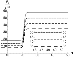
(a)

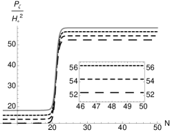
(b)

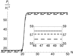
(c)

Figure 5: Impact of different matching prescriptions on the final value of the power spectrum of $\zeta$ in the double-quadratic model (2.7). The quoted value is for the scale which passed outside the horizon with field values $\varphi=8.2M_{\mathrm{P}}$ and $\chi=12.9M_{\mathrm{P}}$, labelled $N=0$ on the figures. In each figure, the short dashed line corresponds to beginning the classical calculation at $N=2$ e-folds after horizon exit; the medium dashed line at $N=4$ e-folds; and the long dashed line at $N=6$ e-folds. The evolution generated by the dynamical renormalization group is the grey solid line. In Fig. LABEL:fig:matching-vary, initial conditions are chosen using $\Sigma_{\alpha\beta}=H^{2}_{N}\delta_{\alpha\beta}$, with $H_{N}$ the value of the Hubble rate at the matching time. In Fig. LABEL:fig:matching-fixed the matching is performed using $\Sigma_{\alpha\beta}=H_{k}^{2}\delta_{\alpha\beta}$, where $H_{k}$ is the value of the Hubble rate at horizon crossing. In Fig. LABEL:fig:matching-nlo the full nlo initial condition (2.4) is used, setting $k_{\ast}=k$ to minimize the $\ln k/k_{\ast}$ terms. In each plot the inset panel shows a close-up of the last four e-folds of evolution.

With the full nlo initial condition (Fig. LABEL:fig:matching-nlo) the discrepancy between the asymptotic value of $P_{\zeta}$ computed using each prescription, and also the drge evolution, is a few percent. In Fig. LABEL:fig:matching-fixed the discrepancy between different matching prescriptions is of order $3\%$–$7\%$. The discrepancy between the $N=6$ prescription and the drge evolution is as large as $10\%$. In Fig. LABEL:fig:matching-vary the discrepancies are very large, between $10\%$ and $40\%$.

In Fig. LABEL:fig:matching-nlo, the expression (3.1) is used to provide an estimate of $\Sigma_{\alpha\beta}$ at the matching surface. One might have expected this estimate to be accurate because it is computed to next-order, and the slow-roll parameters are individually small. Therefore we might also have expected the final difference in $P_{\zeta}$ to be negligible, because the separate universe method is supposed to be independent of the time at which initial conditions are set. The discrepancy arises because, with matching performed at $N>0$, the fixed-order expression is used to evolve $\Sigma_{\alpha\beta}$ up to $N$ e-folds. With the matching performed at $N=0$, all-orders resummation is used. Hence, the non-negligible difference between each line in Fig. LABEL:fig:matching-nlo measures the discrepancy between the resummed and fixed-order calculations. It would be even more significant if these first $N$ e-folds coincided with stronger evolution, such as that occuring near the spike in Fig. 1.

drge analysis.

As observations improve, an ambiguity of order $10\%$ will certainly be important. Therefore we would like to understand which of these prescriptions, if any, is correct. This question cannot be answered within a classical framework. The resolution is that there is no requirement to divide the calculation into ‘quantum’ and ‘classical’ eras joined by a matching condition. Although this is a useful picture which guides our thinking, the calculation can be carried out entirely within the framework of quantum field theory and yields a unique answer. Indeed, as we have seen in §§2–4, the relevant division is not into ‘quantum’ and ‘classical’ effects, but ‘hard’ and ‘soft’ processes. It simply happens that, because interference effects are absent in the soft superhorizon evolution, it can be described at tree-level using the classical equations of motion. In the quantum field theory calculation there is no arbitrary matching between ‘quantum’ and ‘classical’ eras, but only the floating factorization scale. Changes in the factorization scale leave all correlation functions invariant.

The renormalization-group approach we have described allows each correlation function to be calculated purely using the methods of quantum field theory and therefore provides a unique resolution of this matching ambiguity. The prescription can be extracted from Eqs. (4.6) and (4.7). Positive powers of $k\tau$ harmlessly decay and do not contribute to the Taylor series in $\ln(-k_{\ast}\tau)$ at late times. When reversing-engineering this Taylor expansion, the renormalization group evolution should begin at the expansion point $k_{\ast}$ and the initial condition should be the constant term in the Taylor series. As we argued in §4.1, to obtain the most accurate answer we should evaluate (4.7) at the horizon-crossing time for $k$. Therefore we should simultaneously begin the renormalization-group evolution at this time. Hence the prescription provided by the drge is to use the initial condition $\Sigma_{\alpha\beta}\approx H_{k}^{2}\delta_{\alpha\beta}$ but to begin the ‘classical’ evolution at $N=0$. If desired, higher-order corrections can be retained to give a more accurate estimate of the initial value. This has been done to obtain the grey lines in Fig. 5, although the change due to inclusion of nlo terms in the drge initial condition is only of order $0.3\%$.

The prescription provided by the dynamical renormalization group is incompatible with classical intuition, but by itself this is not important because no classical phase of evolution is being invoked in this calculation.

5.2 Nontrivial field-space metric

Elliston et al. [22] recently calculated the inflationary bispectrum generated by a $\sigma$-model Lagrangian with nontrivial field-space metric. The action is

$$S=\frac{1}{2}\int\mathrm{d}^{3}x\,\mathrm{d}t\;a^{3}\Big{[}M_{\mathrm{P}}^{2}R-\bm{\mathrm{G}}_{\alpha\beta}\partial_{a}\phi^{\alpha}\partial^{a}\phi^{\beta}-2V\Big{]}$$ (5.2)

where $V$ is a potential and $\bm{\mathrm{G}}_{\alpha\beta}$ is an arbitrary symmetric matrix which can be interpreted as a metric.

To preserve manifest covariance with respect to $\bm{\mathrm{G}}_{\alpha\beta}$ it is helpful to describe fluctuations using a variable which obeys a covariant transformation law [76, 77]. Gong & Tanaka gave a prescription for rewriting inflationary perturbation theory in terms of such a variable, which they denoted $Q^{\alpha}$, and computed the action for field fluctuations to third-order [77].

Two-point function.

The equal-time two-point function for $Q^{\alpha}$ had already been obtained to leading order by Sasaki & Stewart [15]. The analogue of (2.4) was computed by Nakamura & Stewart [35]. There is a correction to the mass matrix and a more complex structure due to preservation of manifest covariance,

$$\begin{split}\langle Q^{\alpha}(\bm{\mathrm{{k}}}_{1})&Q^{\beta}(\bm{\mathrm{{k}}}_{2})\rangle\supseteq(2\pi)^{3}\delta(\bm{\mathrm{{k}}}_{1}+\bm{\mathrm{{k}}}_{2})\frac{H_{\ast}^{2}}{2k^{3}}{\bm{\Pi}^{\alpha}}_{i}{\bm{\Pi}^{\beta}}_{j}\\ &\times\left\{\bm{\mathrm{G}}^{ij}\left[1+2\varepsilon_{\ast}\left(1-\gamma_{\mathrm{E}}-\ln\frac{2k}{k_{\ast}}\right)\right]+2\bm{\mathrm{w}}^{ij}\left[2-\ln(-k_{\ast}\tau)-\ln\frac{2k}{k_{\ast}}-\gamma_{\mathrm{E}}\right]\right\}.\end{split}$$ (5.3)

In accordance with our usual convention we have neglected decaying power-law corrections. Greek indices $\alpha$, $\beta$, … label the tangent space at field-space coordinate $\phi^{\alpha}(\tau)$, whereas indices $i$, $j$, … label the tangent space at coordinate $\phi^{\alpha}(\tau_{\ast})$, where $\tau_{\ast}$ is the horizon-crossing time for a reference scale $k_{\ast}$. The expansion tensor $\bm{\mathrm{w}}_{ij}$ satisfies

$$\bm{\mathrm{w}}_{ij}=-\frac{V_{ij}}{3H^{2}}+\frac{1}{3H^{2}}\frac{1}{a^{3}}\frac{\mathrm{D}}{\mathrm{d}t}\left(\frac{a^{3}}{H}\dot{\phi}_{i}\dot{\phi}_{j}\right)+\frac{1}{3}\bm{\mathrm{R}}_{imnj}\frac{\dot{\phi}^{m}}{H}\frac{\dot{\phi}^{n}}{H}.$$ (5.4)

The indices $i$, $j$ imply that (5.4) is evaluated at time $\tau_{\ast}$. The same applies for $\bm{\mathrm{G}}_{ij}$. The derivative $\mathrm{D}/\mathrm{d}t$ is $\dot{\phi}^{\alpha}\nabla_{\alpha}$, where $\nabla_{\alpha}$ is the covariant derivative compatible with $\bm{\mathrm{G}}_{\alpha\beta}$ and $\bm{\mathrm{R}}_{\alpha\beta\gamma\delta}$ is the corresponding Riemann tensor. Finally, the parallel propagator ${\bm{\Pi}^{\alpha}}_{i}$ expresses parallel transport along the inflationary trajectory in field-space between $\phi^{\alpha}(\tau_{\ast})$ and $\phi^{\alpha}(\tau)$,

$${\bm{\Pi}^{\alpha}}_{i}=\operatorname{\mathsf{T}}\exp\Big{(}-\int_{\tau_{\ast}}^{\tau}\mathrm{d}\eta\;\Gamma^{\alpha^{\prime}}_{\beta^{\prime}\gamma^{\prime}}\mathrm{d}\phi^{\beta^{\prime}}\Big{)}\delta^{\gamma^{\prime}}_{i}.$$ (5.5)

Indices $\alpha^{\prime}$, $\beta^{\prime}$, … label the tangent space associated with the integration time $\eta$, and $\operatorname{\mathsf{T}}$ is the time-ordering operator. For all details we refer to Elliston et al. [22].

Three-point function.

The equal-time three-point function for $Q^{\alpha}$ was obtained up to $\operatorname{O}(\dot{\phi}/H)^{2}$ in Ref. [22]. It is

$$\langle Q^{\alpha}(\bm{\mathrm{{k}}}_{1})Q^{\beta}(\bm{\mathrm{{k}}}_{2})Q^{\gamma}(\bm{\mathrm{{k}}}_{3})\rangle\supseteq(2\pi)^{3}\delta(\bm{\mathrm{{k}}}_{1}+\bm{\mathrm{{k}}}_{2}+\bm{\mathrm{{k}}}_{3})\frac{H_{\ast}^{4}}{4\prod_{i}k_{i}^{4}}{\bm{\Pi}^{\alpha}}_{i}{\bm{\Pi}^{\beta}}_{j}{\bm{\Pi}^{\gamma}}_{k}A^{ijk}(N),$$ (5.6)

where $A^{ijk}$ transforms as a three-tensor in the tangent space at time $\tau_{\ast}$ and is defined by

$$\begin{split}A^{ijk}=\mbox{}&\frac{1}{M_{\mathrm{P}}^{2}}\frac{\dot{\phi}^{i}}{H}\bm{\mathrm{G}}^{jk}\bigg{(}\frac{k_{1}}{2}\bm{\mathrm{{k}}}_{2}\cdot\bm{\mathrm{{k}}}_{3}-2\frac{k_{2}^{2}k_{3}^{2}}{k_{t}}\bigg{)}\\ &\mbox{}+\frac{4}{3}{\bm{\mathrm{R}}}^{i(jk)m}\frac{\dot{\phi}_{m}}{H}\bigg{[}k_{1}^{3}\Big{(}\gamma_{\mathrm{E}}+\ln(-k_{\ast}\tau)+\ln\frac{k_{t}}{k_{\ast}}\Big{)}-k_{1}^{2}k_{t}+\frac{k_{1}^{2}k_{2}k_{3}}{k_{t}}\bigg{]}\\ &\mbox{}+\frac{1}{3}\nabla^{(i}{\bm{\mathrm{R}}}^{j|mn|k)}\frac{\dot{\phi}_{m}}{H}\frac{\dot{\phi}_{n}}{H}\bigg{[}-k_{1}^{3}\Big{(}\ln(-k_{\ast}\tau)+\ln\frac{k_{t}}{k_{\ast}}+\gamma_{\mathrm{E}}+\frac{1}{3}\Big{)}+\frac{4}{9}k_{t}^{3}-k_{t}K^{2}\bigg{]}\\ &\mbox{}-\frac{4}{3}\nabla^{n}{\bm{\mathrm{R}}}^{i(jk)m}\frac{\dot{\phi}_{m}}{H}\frac{\dot{\phi}_{n}}{H}\bigg{[}\frac{k_{1}^{3}}{2}\Big{(}\ln^{2}(-k_{\ast}\tau)-\gamma_{\mathrm{E}}^{2}+\frac{\pi^{2}}{12}-\Big{[}2\gamma_{\mathrm{E}}+\ln\frac{k_{t}}{k_{\ast}}\Big{]}\ln\frac{k_{t}}{k_{\ast}}\Big{)}\\ &\mbox{}\hskip 108.12047pt+k_{1}^{2}k_{t}\Big{(}\ln\frac{k_{t}}{k_{\ast}}+\gamma_{\mathrm{E}}-1\Big{)}-\frac{k_{1}^{2}k_{2}k_{3}}{k_{t}}\Big{(}\gamma_{\mathrm{E}}+\ln\frac{k_{t}}{k_{\ast}}\Big{)}\bigg{]}\\ &\mbox{}+\text{cyclic}.\end{split}$$ (5.7)

We have used $k_{t}=k_{1}+k_{2}+k_{3}$ and $K^{2}=\sum_{i<j}k_{i}k_{j}=k_{1}k_{2}+k_{1}k_{3}+k_{2}k_{3}$. As in (5.4), all time-dependent quantities are evaluated at the horizon-crossing time for $k_{\ast}$.

Eqs. (5.6)–(5.7) are considerably more complicated than their flat field-space counterparts. Growing terms involving $\ln(-k_{\ast}\tau)$ are already present at lowest nontrivial order in $\dot{\phi}/H$. At $\operatorname{O}(\dot{\phi}/H)^{2}$ a double-logarithmic term involving $\ln^{2}(-k_{\ast}\tau)$ appears. In flat field-space, growing terms appear only at $\operatorname{O}(\dot{\phi}/H)^{3}$ and double logarithms do not occur until even higher orders. In combination with the propagator terms ${\bm{\Pi}^{\alpha}}_{i}$ these make the time dependence of (5.6) appear extremely complicated.

Dynamical renormalization group analysis.

Eqs. (5.3), (5.6) and (5.7) present a case study in the use of renormalization group techniques to extract a Sudakov-like structure from logarithmic divergences.

The Taylor theorem on a curved manifold is

$${A^{\alpha\cdots}}_{\beta\cdots}(x)={\bm{\Pi}^{\alpha}}_{\alpha^{\prime}}(x,x^{\prime})\cdots{\bm{\Pi}_{\beta}}^{\beta^{\prime}}(x,x^{\prime})\cdots\left[{A^{\alpha^{\prime}\cdots}}_{\beta^{\prime}\cdots}\Big{|}_{x^{\prime}}+\frac{\mathrm{D}}{\mathrm{d}\lambda}{A^{\alpha^{\prime}\cdots}}_{\beta^{\prime}\cdots}\bigg{|}_{x^{\prime}}\delta\lambda+\cdots\right],$$ (5.8)

where the omitted terms are $\operatorname{O}(\delta\lambda^{2})$. To write (5.8) we have assumed a smooth path connecting $x$ and $x^{\prime}$, with ${\bm{\Pi}^{\alpha}}_{\alpha^{\prime}}(x,x^{\prime})$ the parallel propagator along this path and $\mathrm{D}/\mathrm{d}\lambda$ the corresponding parametric derivative. As in §4, the Taylor theorem (5.8) is our principal tool in the renormalization-group analysis. The path connecting $x$ and $x^{\prime}$ will be the inflationary trajectory, and the parametric derivative along it will be $\mathrm{D}/\mathrm{d}N$.

The argument now parallels §4 precisely. Comparing Eq. (5.3) with (5.8) allows us to conclude

$$\frac{\mathrm{D}}{\mathrm{d}N}\Sigma^{\alpha\beta}\bigg{|}_{-k_{\ast}\tau=1}=2H^{2}\bm{\mathrm{w}}^{\alpha\beta}\Big{|}_{-k_{\ast}\tau=1}.$$ (5.9)

The arbitrariness of $k_{\ast}$ allows this to be promoted to a differential equation. Replacing $H_{\ast}$ by suitable copies of $\Sigma_{\alpha\beta}$, as in §4, we find

$$\frac{\mathrm{D}\Sigma^{\alpha\beta}}{\mathrm{d}N}={\bm{\mathrm{w}}^{\alpha}}_{\gamma}\Sigma^{\gamma\beta}+{\bm{\mathrm{w}}^{\beta}}_{\gamma}\Sigma^{\gamma\alpha}.$$ (5.10)

A similar analysis can be performed for the three-point function. Eq. (5.7) shows that all time-dependent logarithms multiply only local momentum shapes, in agreement with the factorization theorem of §4.2. (This is not altered by the presence of a nontrivial metric.) Repeating the argument of §4.3, we conclude

$$\frac{\mathrm{D}a_{\alpha|\beta\gamma}}{\mathrm{d}N}={\bm{\mathrm{w}}_{\alpha}}^{\lambda}a_{\lambda|\beta\gamma}+{\bm{\mathrm{w}}_{\beta}}^{\lambda}a_{\alpha|\lambda\gamma}+{\bm{\mathrm{w}}_{\gamma}}^{\lambda}a_{\alpha|\beta\lambda}+{\bm{\mathrm{w}}_{\alpha}}^{\lambda\mu}\Sigma_{\lambda\beta}\Sigma_{\mu\gamma},$$ (5.11)

where $\bm{\mathrm{w}}_{\alpha\beta\gamma}$ satisfies

$$\bm{\mathrm{w}}_{\alpha\beta\gamma}=\nabla_{(\alpha}\bm{\mathrm{w}}_{\beta\gamma)}+\frac{1}{3}\left(\nabla_{(\alpha}{\bm{\mathrm{R}}}_{\beta|\lambda\mu|\gamma)}\frac{\dot{\phi}^{\lambda}}{H}\frac{\dot{\phi}^{\mu}}{H}-4{\bm{\mathrm{R}}}_{\alpha(\beta\gamma)\lambda}\frac{\dot{\phi}^{\lambda}}{H}\right).$$ (5.12)

Jacobi equation.

Elliston et al. deduced equations equivalent to (5.10) and (5.11)–(5.12) from the evolution of a covariant connecting vector between two adjacent inflationary trajectories [22], and demonstrated that (when solved perturbatively) these transport equations reproduce the ‘divergences’ involving $\ln(-k_{\ast}\tau)$ and $\ln^{2}(-k_{\ast}\tau)$ in (5.3) and (5.6)–(5.7). The analysis in this section shows that this agreement is not restricted to the lowest powers of $\ln(-k_{\ast}\tau)$ but will extend to the leading-logarithm terms at all orders.

Comparing the analysis of Elliston et al. [22] with the discussion given in this section highlights the advantages and disadvantages of the renormalization-group technique. Eqs. (5.10)–(5.12) involve combinations of the Riemann curvature tensor and its derivative which one could not expect to obtain by accident. The analysis of Elliston et al. [22] provides an explanation for the precise combinations which appear, and shows how they can be understood in geometrical terms. On its own, however, it does not demonstrate agreement to higher orders in $\ln(-k_{\ast}\tau)$. This is important, because as we argued in §2 and was demonstrated explicitly in Fig. LABEL:fig:matching-nlo, contributions from all powers of $\ln(-k_{\ast}\tau)$ are required to obtain an accurate prediction.

In contrast, by combining the dynamical renormalization-group framework with a factorization theorem, we derived a correct set of transport equations directly from the linear $\ln(-k_{\ast}\tau)$ ‘divergences’. (As we explained in footnote 7 on p. 7, there is no need to take special measures to account for the double-logarithmic term.) Therefore the drge procedure gives an algorithmic method to obtain a correct evolution equation, valid to leading-logarithm order. But conversely it gives no information about the physical interpretation of this evolution, in the same way that the successful calculation of a negative $\beta$-function in QCD did not directly give an interpretation of asymptotic freedom as a consequence of antiscreening due to gluonic fluctuations.

In this case Elliston et al. were able to guess the correct physical interpretation of Eqs. (5.10) and (5.11)–(5.12). But it is easy to imagine that, in more complex circumstances (perhaps where the effect of time-dependence from loop corrections is included), it would no longer be possible to guess the correct evolution equation using simple physical arguments. In such cases the dynamical renormalization group provides a straightforward and algorithmic approach. In canonical models it requires the extra complexity of a next-order calculation to obtain the first contributions to the linear term in the Taylor expansion [that is, the term proportional to $\ln(-k_{\ast}\tau)$]. For the nontrivial metric, the relevant new terms involving the Riemann curvature appear already at lowest order.

6 Summary and discussion

The separate universe picture is a powerful method to compute the superhorizon evolution of inflationary correlation functions. Our main result is a derivation of this method from the renormalization group technique. We have focused on the bispectrum, where the simplest discussion can be given, but it is clear what would be involved in extending the analysis to higher $n$-point functions.

The main steps in the argument are simple. We first show that the vertex integral obeys a ‘factorization’ principle: to all orders in the slow-roll expansion, time-dependent logarithms appear only in combination with a few fixed functions of the external momenta. The second step is to derive renormalization-group equations for the coefficients of these fixed functions. These equations turn out to be the transport equations for the two- and three-point functions, which were shown in Ref. [18] to be equivalent to the separate-universe Taylor expansion introduced by Lyth & Rodríguez. Therefore, in combination, the factorization principle and RGE approach reproduce the separate universe method. Technically our argument demonstrates this in the leading-logarithm approximation.

Our result suggests a systematic method to incorporate more than the lowest-order contribution to each correlation function. Burgess et al. [12] studied time-dependent effects from loop-level corrections to the power spectrum, making use of the same dynamical renormalization group methods employed in §4. More recently, Collins et al. [63] studied effective field theories in a nonequilibrium or time-dependent setting, finding nontrivial contributions to the time-dependence after integrating out a massive field. To perform calculations analogous to these for $n$-point functions with $n\geqslant 3$ during an inflationary phase it would be necessary to proceed as in §4—first, proving a suitable factorization theorem; and second, constructing the relevant renormalization-group equation. (For the two-point function, factorization is usually a much more straightforward question due to the absence of vertex integrals.)

The factorization property admits a clear physical interpretation which is related to the usual division of separate-universe calculations into a quantum contribution, generated near horizon-crossing, followed by classical evolution. The renormalization-group analysis gives a sharper version of this division. Fluctuations are created as they inflate beyond the Hubble length, on a timescale which is rapid compared to their subsequent evolution and which is insensitive to any model-dependent parameters. Factorization divides the physics of the fluctuations into two parts: a ‘hard’ model-independent subprocess associated with the creation event, and ‘soft’, model-dependent interactions which subsequently dress the hard subprocess. One way to understand why correlation functions factorize into self-contained parts associated with these ‘hard’ and ‘soft’ processes is that the disparity in timescales prevents interference effects between the two.

Because we work to tree-level, it follows that the soft physics can be described using the classical equations of motion. Had we chosen to compute beyond tree-level, the applicability of classical equations of motion might be lost but the division into hard and soft physics would remain. Therefore, as a conceptual tool, the hard/soft division takes the place of the usual quantum/classical separation, allowing correlation functions to be calculated without invoking any classical phase at all. Naturally, this does not absolve us of the obligation to explain why the correlation functions obtained in this way can subsequently be re-interpreted as the correlations of a classical stochastic process—that is, why we see fluctuations which behave classically. The renormalization-group method has nothing new to say about this difficulty.

In the course of our analysis we treated all fields as perturbatively massless. (That is, mass terms are treated as interactions.) This has two important consequences. First, all $k$-dependence occurs as integer power laws modified by logarithms. For example, $k^{3+\delta}\approx k^{3}[1+\delta\ln k+\operatorname{O}(\delta^{2})]$; it is the infinite sum of logarithms which reproduces a power-law scaling. This restriction to integer powers of $k$ was helpful in proving the factorization theorem in §4.2, which depended on the existence of a ‘gap’ in the asymptotic expansion of each wavefunction in integer powers of $k$, Eq. (4.8). In our applications, the coefficient $\delta$ is of order a slow-roll parameter, so in a strict mathematical interpretation we are restricted to scenarios in which the slow-roll parameters are small throughout the evolution. Second, the appearance of time-dependent logarithmic ‘divergences’ of the form $\ln(-k_{\ast}\tau)$ is itself a consequence of the massless approximation. Incorporation of masses would provide a cutoff which prevents these terms growing unboundedly.

Finally, it should be remembered that our analysis does not apply to all theories. Scenarios which contain other distinguished scales need not satisfy the conditions of the factorization theorem proved in §4.2. To obtain this theorem it was assumed that asymptotic information about the wavefunctions provided all necessary data about the superhorizon regime. Where this assumption fails, other combinations of the external momenta could receive significant enhancements. This corresponds to the well-known restriction that, in applying separate-universe arguments, all relevant scales should first be outside the horizon.

Appendix A Three-point function at next-to-leading order

In this Appendix we collect the components of the three-point function up to nlo in the slow-roll expansion, and briefly sketch some details of its calculation. For full details of the ‘in–in’ or ‘Schwinger–Keldysh’ method used to obtain inflationary correlation functions we refer to the literature [1, 68, 78, 51, 52].

A.1 Propagator

We require the second- and third-order action for a collection of light, canonically-normalized scalar fields coupled to gravity. The second-order action has already been given in (2.1). To obtain the propagator $G$, defined in conformal time by

$$G^{\alpha\beta}(\bm{\mathrm{{x}}},\tau;\tilde{\bm{\mathrm{{x}}}},\tilde{\tau})=\langle\delta\phi^{\alpha}(\bm{\mathrm{{x}}},\tau)\delta\phi^{\beta}(\tilde{\bm{\mathrm{{x}}}},\tilde{\tau})\rangle,$$ (A.1)

we should invert the quadratic structure appearing in the action. That gives

$$\left\{\delta_{\alpha\beta}\left(\frac{\partial^{2}}{\partial\tau^{2}}+2\frac{\partial\ln a}{\partial\tau}\frac{\partial}{\partial\tau}-\partial^{2}\right)+a^{2}m_{\alpha\beta}\right\}G^{\beta\gamma}=-\frac{\mathrm{i}}{a^{2}}\delta^{\gamma}_{\alpha}\ \delta(\bm{\mathrm{{x}}}-\tilde{\bm{\mathrm{{x}}}})\delta(\tau-\tilde{\tau}).$$ (A.2)

Because spatial translations and rotations are unbroken by the de Sitter background, $G$ can depend only on the relative displacement $\bm{\mathrm{{x}}}-\tilde{\bm{\mathrm{{x}}}}$. Diagonalizing this by passing to Fourier space,

$$G^{\alpha\beta}(\tau,\tilde{\tau};\bm{\mathrm{{x}}}-\tilde{\bm{\mathrm{{x}}}})=\int\frac{\mathrm{d}^{3}k}{(2\pi)^{3}}\ G^{\alpha\beta}_{k}(\tau,\tau^{\prime})\mathrm{e}^{{\mathrm{i}\bm{\mathrm{{k}}}\cdot(\bm{\mathrm{{x}}}-\tilde{\bm{\mathrm{{x}}}})}},$$ (A.3)

and introducing a dimensionless time $y=k\tau=-k/aH$, we find

$$\left\{\delta_{\alpha\beta}\left(\frac{\mathrm{d}^{2}}{\mathrm{d}y^{2}}+2\frac{a^{\prime}}{a}\frac{\mathrm{d}}{\mathrm{d}y}+1\right)+\frac{a^{2}}{k^{2}}m_{\alpha\beta}\right\}G^{\beta\gamma}_{k}=-\frac{\mathrm{i}}{ka^{2}}\delta^{\gamma}_{\alpha}\ \delta(y-\tilde{y}),$$ (A.4)

where $\tilde{y}=k\tilde{\tau}$ and $a^{\prime}$ now denotes $\mathrm{d}a/\mathrm{d}x$. Eq. (A.4) can be transformed into a Bessel equation by making the substitution $G^{\alpha\beta}_{k}=w^{\alpha\beta}\sqrt{-y}/a$. After expanding $a$ to next-order (for details, see Refs. [79, 8]) we finally arrive at an equation which can be solved perturbatively,

$$\left\{\delta_{\alpha\beta}\left(\frac{\mathrm{d}^{2}}{\mathrm{d}y^{2}}+\frac{1}{y}\frac{\mathrm{d}}{\mathrm{d}y}+\left[1-\frac{9/4}{y^{2}}\right]\right)-\frac{3M_{\alpha\beta}}{y^{2}}\right\}w^{\beta\gamma}=-\frac{\mathrm{i}}{ka\sqrt{-y}}\delta^{\gamma}_{\alpha}\ \delta(y-\tilde{y}),$$ (A.5)

where $M_{\alpha\beta}=\varepsilon_{\ast}\delta_{\alpha\beta}+u_{\alpha\beta}$ was defined in Eq. (3.2b). It plays the role of an effective mass term, including contributions from coupling to the background geometry.

Homogeneous solution.

The technology to solve Eq. (A.5) perturbatively in $M_{\alpha\beta}$ was developed by Nakamura & Stewart [35] and Gong & Stewart [36, 37]. We adopt their methods, with some small modifications noted below to keep each wavefunction purely imaginary in the late-time limit. The first step is to find a solution $v^{\beta\gamma}$ of the homogeneous equation,

$$\left\{\delta_{\alpha\beta}\left(\frac{\mathrm{d}^{2}}{\mathrm{d}y^{2}}+\frac{1}{y}\frac{\mathrm{d}}{\mathrm{d}y}+\left[1-\frac{9/4}{y^{2}}\right]\right)-\frac{3M_{\alpha\beta}}{y^{2}}\right\}v^{\beta\gamma}=0.$$ (A.6)

To do so we work perturbatively in $M_{\alpha\beta}$, writing $v^{\alpha\beta}=v_{0}^{\alpha\beta}+v_{1}^{\alpha\beta}+\cdots$, with $v_{n}^{\alpha\beta}=\operatorname{O}(M^{n})$. Up to $\operatorname{O}(M)$ we find

$$\delta_{\alpha\beta}\left(\frac{\mathrm{d}^{2}}{\mathrm{d}y^{2}}+\frac{1}{y}\frac{\mathrm{d}}{\mathrm{d}y}+\left[1-\frac{9/4}{y^{2}}\right]\right)v_{0}^{\beta\gamma} =0,$$ (A.7a)

$$\delta_{\alpha\beta}\left(\frac{\mathrm{d}^{2}}{\mathrm{d}y^{2}}+\frac{1}{y}\frac{\mathrm{d}}{\mathrm{d}y}+\left[1-\frac{9/4}{y^{2}}\right]\right)v_{1}^{\beta\gamma} =\frac{3}{y^{2}}M_{\alpha\beta}v_{0}^{\beta\gamma}.$$ (A.7b)

Eq. (A.7a) has solution in terms of Bessel functions of order $3/2$. The linear combination with correct boundary conditions to match the Minkowski-space wavefunctions in the subhorizon limit $k/aH=|y|\rightarrow\infty$ is the Hankel function,

$$v_{0}^{\alpha\beta}=\mathcal{U}^{\alpha\beta}H_{3/2}^{(2)}(-k\tau)$$ (A.8)

where $\mathcal{U}^{\alpha\beta}$ is an arbitrary constant matrix. Eq. (A.7b) can be solved using the causal Green’s function $\Gamma(y,z)$ constructed by Gong & Stewart [36, 37]. This satisfies

$$\frac{\mathrm{d}^{2}\Gamma}{\mathrm{d}y^{2}}+\frac{1}{y}\frac{\mathrm{d}\Gamma}{\mathrm{d}y}+\left[1-\frac{9/4}{y^{2}}\right]\Gamma=\delta(y-z),$$ (A.9)

and can be written explicitly in terms of the Hankel functions

$$\Gamma(y,z)=-\frac{\mathrm{i}\pi z}{4}\times\begin{cases}0&y<z\\ H_{3/2}^{(2)}(-y)H_{3/2}^{(1)}(-y)-H_{3/2}^{(1)}(-y)H_{3/2}^{(2)}(-y)&y>z\end{cases}\quad.$$ (A.10)

After integrating over $\Gamma$, the solution $v_{1}^{\alpha\beta}$ can be written

$$v^{\alpha\beta}_{1}={M^{\alpha}}_{\gamma}\ \mathcal{U}^{\gamma\beta}\ v_{1},$$ (A.11)

where $v_{1}$ satisfies [36, 37]

$$v_{1}=\mathrm{i}\sqrt{\frac{2}{\pi}}\frac{1}{(-y)^{3/2}}\left(2\mathrm{e}^{{\mathrm{i}y}}-(1+\mathrm{i}y)\mathrm{e}^{{-\mathrm{i}x}}\int_{-\infty}^{y}\frac{\mathrm{d}z}{z}\mathrm{e}^{{2\mathrm{i}z}}\right).$$ (A.12)

In writing (A.11) we have adjusted the position of the indices on $M$ to match on both sides of the equation. However, since we are generally working with a flat field-space metric, except in §5.2, there is no distinction between co- and contravariant indices.

The scalar part of the zero-order wavefunction $H_{3/2}^{(2)}(-y)$ has the property that it is purely imaginary at late times,

$$H_{3/2}^{(2)}(-y)\rightarrow\mathrm{i}\sqrt{\frac{2}{\pi}}\frac{1}{(-y)^{3/2}}+\operatorname{O}(y).$$ (A.13)

However, in this limit $v_{1}$ is complex. Assembling (A.8), (A.11) and (A.12) gives

$$v^{\alpha\beta}\rightarrow\mathrm{i}\sqrt{\frac{2}{\pi}}\frac{1}{(-y)^{3/2}}\left(\mathcal{U}^{\alpha\beta}+{M^{\alpha}}_{\gamma}\ \mathcal{U}^{\gamma\beta}\Big{[}2-\gamma_{\mathrm{E}}-\ln(-2y)-\mathrm{i}\frac{\pi}{2}\Big{]}\right).$$ (A.14)

It is the term involving $\mathrm{i}\pi/2$ which is problematic. This arises from the asymptotic expansion of the exponential integral appearing in Eq. (A.12). We will see below that to clearly exhibit the cancellation of unwanted divergent terms in the calculation of the three-point functions it is helpful to adjust the phase of $v^{\alpha\beta}$ so that this term is removed. Therefore we redefine $v_{\alpha\beta}$ by a pure phase

$$v^{\alpha\beta}\rightarrow\tilde{v}^{\alpha\beta}=\exp(\mathrm{i}\theta^{\alpha\gamma})v^{\gamma\beta},$$ (A.15)

where $\theta^{\alpha\beta}$ is a constant real matrix. This redefinition does not change the propagator, which depends on the combination $\bm{\mathrm{{v}}}^{\dagger}\cdot\bm{\mathrm{{v}}}$ in which this phase cancels out. To remove the imaginary term in Eq. (A.14) we should choose $\theta^{\alpha\beta}=(\pi/2)M^{\alpha\beta}$. The net effect is to replace $v_{1}$ in Eq. (A.12) with a redefined function (cf. Refs. [70, 80, 8])

$$v_{1}\rightarrow\tilde{v}_{1}=\mathrm{i}\sqrt{\frac{2}{\pi}}\frac{1}{(-y)^{3/2}}\left(2\mathrm{e}^{{\mathrm{i}y}}+\mathrm{i}\frac{\pi}{2}(1-\mathrm{i}y)\mathrm{e}^{{\mathrm{i}y}}-(1+\mathrm{i}y)\mathrm{e}^{{-\mathrm{i}y}}\int_{-\infty}^{y}\frac{\mathrm{d}z}{z}\mathrm{e}^{{2\mathrm{i}z}}\right).$$ (A.16)

Feynman propagator.

We now return to Eq. (A.5) and use the homogeneous solution $v^{\alpha\beta}$ to construct the Feynman Green’s function $w^{\alpha\beta}$. In this section it is helpful to switch to matrix notation, with $(\bm{\mathrm{{v}}})_{\alpha\beta}=v^{\alpha\beta}$, $(\bm{\mathrm{{w}}})_{\alpha\beta}=w^{\alpha\beta}$ and so on. In the absence of the mass matrix $\bm{\mathrm{{M}}}$ the field fluctuations are uncorrelated, which implies that we must choose $\bm{\mathrm{{\mathcal{U}}}}=\bm{\mathrm{{1}}}$. Together, the Feynman boundary conditions and hermiticity require

$$\bm{\mathrm{{u}}}=\begin{cases}\bm{\mathrm{{v}}}^{\dagger}(\tilde{y})\cdot\bm{\mathrm{{Y}}}\cdot\bm{\mathrm{{v}}}(y)&y<\tilde{y}\\ \bm{\mathrm{{v}}}^{\dagger}(y)\cdot\bm{\mathrm{{Y}}}\cdot\bm{\mathrm{{v}}}(\tilde{y})&y>\tilde{y}\end{cases}$$ (A.17)

where $\bm{\mathrm{{Y}}}$ is an Hermitian matrix. We will take it to commute with $\bm{\mathrm{{v}}}$ and $\bm{\mathrm{{v}}}^{\dagger}$. This can be justified (with our choice $\bm{\mathrm{{\mathcal{U}}}}=1$) because Eq. (A.6) implies that both $\bm{\mathrm{{v}}}$ and $\bm{\mathrm{{v}}}^{\dagger}$ are power series in the Hermitian matrix $\bm{\mathrm{{M}}}$. The normalization condition in (A.5) likewise guarantees that $\bm{\mathrm{{Y}}}$ is a power series in $\bm{\mathrm{{M}}}$. Therefore all these matrices commute. Imposing this normalization condition, we conclude

$$\bm{\mathrm{{Y}}}\cdot\left(\bm{\mathrm{{v}}}(\tilde{y})\cdot\frac{\mathrm{d}\bm{\mathrm{{v}}}^{\dagger}(\tilde{y})}{\mathrm{d}\tilde{y}}-\bm{\mathrm{{v}}}^{\dagger}(\tilde{y})\cdot\frac{\mathrm{d}\bm{\mathrm{{v}}}(\tilde{y})}{\mathrm{d}\tilde{y}}\right)=-\frac{\mathrm{i}}{(-\tilde{y})^{1/2}ka(\tilde{y})}\times\bm{\mathrm{{1}}}.$$ (A.18)

The matrix in brackets $(\cdots)$ is the ‘Wronskian matrix’ for $\bm{\mathrm{{v}}}$ and $\bm{\mathrm{{v}}}^{\dagger}$. Abel’s theorem shows that it can be written

$$\bm{\mathrm{{W}}}(\tilde{y})=\bm{\mathrm{{v}}}(\tilde{y})\cdot\frac{\mathrm{d}\bm{\mathrm{{v}}}^{\dagger}(\tilde{y})}{\mathrm{d}\tilde{y}}-\bm{\mathrm{{v}}}^{\dagger}(\tilde{y})\cdot\frac{\mathrm{d}\bm{\mathrm{{v}}}(\tilde{y})}{\mathrm{d}\tilde{y}}=\bm{\mathrm{{W}}}(\tilde{y}_{0})\exp\left(-\int_{\tilde{y}_{0}}^{\tilde{y}}\frac{\mathrm{d}z}{z}\right)=\bm{\mathrm{{W}}}(\tilde{y}_{0})\frac{\tilde{y}_{0}}{\tilde{y}},$$ (A.19)

where $\tilde{y}_{0}$ is arbitrary and $\bm{\mathrm{{W}}}(\tilde{y}_{0})$ is independent of $\bm{\mathrm{{M}}}$. With our choice $\bm{\mathrm{{\mathcal{U}}}}=1$, we find

$$\bm{\mathrm{{W}}}(\tilde{y})=-\frac{4\mathrm{i}}{\pi(-\tilde{y})}\times\bm{\mathrm{{1}}}.$$ (A.20)

Therefore $\bm{\mathrm{{Y}}}$ is Hermitian and commutes with $\bm{\mathrm{{M}}}$, in agreement with our earlier argument. In conclusion, the Feynman propagator can be written

$$\bm{\mathrm{{G}}}_{k}=\frac{\pi}{4k}\frac{(-y)^{1/2}(-\tilde{y})^{1/2}}{a(y)a(\tilde{y})}\times\begin{cases}\bm{\mathrm{{v}}}^{\dagger}(\tilde{y})\cdot\bm{\mathrm{{v}}}(y)&y<\tilde{y}\\ \bm{\mathrm{{v}}}^{\dagger}(y)\cdot\bm{\mathrm{{v}}}(\tilde{y})&y>\tilde{y}\end{cases}.$$ (A.21)

Uniform expansion of $\bm{\mathrm{{G}}}_{k}$ to next-order.

We require the lowest-order and next-order contributions in slow-roll to $\bm{\mathrm{{G}}}_{k}$. This can be obtained from the solutions $v_{0}^{\alpha\beta}$ and $v_{1}^{\alpha\beta}$ together with next-order corrections to the scale factor $a$, for which purpose we must Taylor expand around an arbitrary reference scale $k_{\ast}$ as described in §2. Denoting evaluation at the horizon-crossing time for $k_{\ast}$ by a subscript ‘$\ast$’, we find that $\bm{\mathrm{{G}}}_{k}$ behaves like the product of two effective wave-function factors $\bm{\mathrm{{w}}}$,

$$\bm{\mathrm{{G}}}_{k}=\begin{cases}\bm{\mathrm{{w}}}^{\dagger}(\tilde{y})\cdot\bm{\mathrm{{w}}}(y)&y<\tilde{y}\\ \bm{\mathrm{{w}}}^{\dagger}(y)\cdot\bm{\mathrm{{w}}}(\tilde{y})&y>\tilde{y}\end{cases},$$ (A.22)

where $\bm{\mathrm{{w}}}=\bm{\mathrm{{w}}}_{0}+\bm{\mathrm{{w}}}_{1}+\cdots$ satisfies

$$\bm{\mathrm{{w}}}_{0}(y) =\frac{\mathrm{i}}{\sqrt{2k^{3}}}H_{\ast}(1-\mathrm{i}y)\mathrm{e}^{{\mathrm{i}y}}\cdot\bm{\mathrm{{1}}}$$ (A.23a)

$$\begin{split}\bm{\mathrm{{w}}}_{1}(y)&=\frac{\mathrm{i}}{\sqrt{2k^{3}}}H_{\ast}\Big{\{}\varepsilon_{\ast}\Big{[}\big{(}\ln\frac{k_{\ast}}{k}(-y)\big{)}-1\Big{]}(1-\mathrm{i}y)\mathrm{e}^{{\mathrm{i}y}}\cdot\bm{\mathrm{{1}}}\\ &\hskip 62.59596pt\mbox{}+\bm{\mathrm{{M}}}\cdot\Big{[}2\mathrm{e}^{{\mathrm{i}y}}+\mathrm{i}\frac{\pi}{2}(1-\mathrm{i}y)\mathrm{e}^{{\mathrm{i}y}}-(1+\mathrm{i}y)\mathrm{e}^{{-\mathrm{i}y}}\int_{-\infty}^{y}\frac{\mathrm{d}z}{z}\mathrm{e}^{{2\mathrm{i}z}}\Big{]}\Big{\}}.\end{split}$$ (A.23b)

[This result was used in the main text in Eq. (3.6).] Eqs. (A.23a) and (A.23b) are both exact in $y$ but perturbative in powers of slow-roll and mass $\bm{\mathrm{{M}}}$.

A.2 Asymptotic behaviour of wavefunctions

In practical calculations we require the late-time expansion of the elementary wavefunctions, $\bm{\mathrm{{w}}}$, in order to compute the contribution from external lines. In the present case it is only necessary to compute these up to $\operatorname{O}(y^{2})$. We find

$$\bm{\mathrm{{w}}}(y)=\dfrac{\mathrm{i}}{\sqrt{2k^{3}}}H_{\ast}\mathrm{e}^{{\mathrm{i}y}}\Big{\{}\bm{\mathrm{{1}}}+\bm{\mathrm{{A}}}_{\ast}-\bm{\mathrm{{u}}}\ln\frac{k_{\ast}}{k}(-y)-\mathrm{i}y\big{(}\bm{\mathrm{{1}}}+\bm{\mathrm{{A}}}_{\ast}\big{)}+\mathrm{i}y\bm{\mathrm{{u}}}\ln\frac{k_{\ast}}{k}(-y)+\operatorname{O}(y)^{2}\Big{\}}\ ,$$ (A.24)

where

$$\bm{\mathrm{{A}}}\equiv\varepsilon_{\ast}\Big{(}1-\gamma_{\mathrm{E}}-\ln\frac{2k}{k_{\ast}}\Big{)}\bm{\mathrm{{1}}}+\bm{\mathrm{{u}}}_{\ast}\Big{(}2-\gamma_{\mathrm{E}}-\ln\frac{2k}{k_{\ast}}\Big{)},$$ (A.25)

and $\bm{\mathrm{{u}}}$ is defined in Eq. (2.3).

A.3 Three-point function

To compute the three-point function we require the action to third-order. This calculation is well-documented in the literature; see, for examples, Refs. [1, 23]. Fluctuations in the fields will mix with the metric, which can be accommodated using the ADM decomposition (4.12)

$$\mathrm{d}s^{2}=-N^{2}\,\mathrm{d}t^{2}+h_{ij}(\mathrm{d}x^{i}+N^{i}\,\mathrm{d}t)(\mathrm{d}x^{j}+N^{j}\,\mathrm{d}t),$$ (A.26)

where the lapse $N$ and shift vector $N^{i}$ are determined by constraint equations which follow from invariance under temporal and spatial reparametrizations. At the level of the background we have $N=1$ and $N^{i}=0$. When perturbations are included there are order-by-order corrections, discussed in §4.2.4,

$$N =1+\sum_{n=1}^{\infty}\alpha_{n},$$ (A.27a)

$$N_{i} =\sum_{n=1}^{\infty}\partial_{i}\vartheta_{n}+\text{solenoidal component}.$$ (A.27b)

The solenoidal part of $N_{i}$ is important only when computing the action at fourth-order and above [81, 82]. (Spatial indices $i$, $j$, … are raised and lowered using the three-metric $h_{ij}$.) Also, although in principle there could be contributions to the third-order action from $\alpha_{n}$ and $\vartheta_{n}$ with $n\leqslant 3$, the structure of the constraints in the action guarantees that only $\alpha_{1}$ and $\vartheta_{1}$ contribute [1, 70]. Specializing to the spatially flat gauge $h_{ij}=a^{2}\delta_{ij}$, we find

$$\begin{split}S_{\phi\phi\phi}\supseteq\frac{1}{2}\int\mathrm{d}^{3}x\,\mathrm{d}t\;a^{3}\bigg{\{}&-\frac{1}{3}V_{\alpha\beta\gamma}\delta\phi^{\alpha}\delta\phi^{\beta}\delta\phi^{\gamma}-\frac{2}{a^{2}}\delta\dot{\phi}^{\alpha}\partial_{j}\vartheta_{1}\partial_{j}\delta\phi_{\alpha}\\ &\mbox{}+\alpha_{1}\Big{[}-\frac{1}{a^{2}}\partial_{j}\delta\phi^{\alpha}\partial_{j}\delta\phi_{\alpha}-\delta\dot{\phi}^{\alpha}\delta\dot{\phi}_{\alpha}-V_{\alpha\beta}\delta\phi^{\alpha}\delta\phi^{\beta}\\ &\hskip 31.0134pt\mbox{}-\frac{1}{a^{4}}\partial_{i}\partial_{j}\vartheta_{1}\partial_{i}\partial_{j}\vartheta_{1}+\frac{1}{a^{4}}\partial^{2}\vartheta_{1}\partial^{2}\vartheta_{1}+\frac{2}{a^{2}}\dot{\phi}^{\alpha}\partial_{j}\vartheta_{1}\partial_{j}\delta\phi_{\alpha}\\ &\hskip 31.0134pt\mbox{}+\alpha_{1}\Big{(}2\dot{\phi}^{\alpha}\delta\dot{\phi}_{\alpha}+\frac{4H}{a^{2}}\partial^{2}\vartheta_{1}+\alpha_{1}(6H^{2}-\dot{\phi}^{2})\Big{)}\Big{]}\bigg{\}}\end{split}$$ (A.28)

where $\dot{\phi}^{2}=\dot{\phi}_{\alpha}\dot{\phi}_{\alpha}$ and repeated indices in the lower position are summed using the flat Euclidean metric $\delta_{ij}$. Eq. (A.28) is exact. It has been obtained using an expansion in the amplitudes $|\delta\phi|$ but does not invoke an expansion in slow-roll parameters. The solution for $\alpha_{1}$ is

$$\alpha_{1}=\frac{\dot{\phi}_{\alpha}\delta\phi_{\alpha}}{2H},$$ (A.29)

and the solution for $\vartheta_{1}$ was used in (4.13),

$$\frac{4H}{a^{2}}\partial^{2}\vartheta_{1}=-2V_{\alpha}\delta\phi_{\alpha}-2\dot{\phi}_{\alpha}\delta\dot{\phi}_{\alpha}+2\alpha_{1}(-6H^{2}+\dot{\phi}^{2}).$$ (A.30)

We wish to compute the three-point function up to terms which are next-to-leading (‘nlo’) in a fixed-order slow-roll expansion. For this purpose we need only extract the lo and nlo terms in (A.28). The lo contributions were given in Ref. [23], where the corresponding three-point function was also obtained. They are

$$S^{\text{{lo}}}_{\phi\phi\phi}\supseteq\frac{1}{2}\int\mathrm{d}^{3}x\,\mathrm{d}t\;a^{3}\bigg{(}\frac{1}{H}\dot{\phi}^{\beta}\delta\dot{\phi}^{\alpha}\partial_{j}\delta\phi_{\alpha}\partial_{j}\partial^{-2}\delta\dot{\phi}_{\beta}-\alpha_{1}\Big{[}\delta\dot{\phi}^{\alpha}\delta\dot{\phi}_{\alpha}+\frac{1}{a^{2}}\partial_{j}\delta\phi^{\alpha}\partial_{j}\delta\phi_{\alpha}\Big{]}\bigg{)}\ \ ,$$ (A.31)

(In Ref. [23] the action was quoted in a different but equivalent form.) The new contributions at nlo are

$$\begin{split}S^{\text{{nlo}}}_{\phi\phi\phi}\supseteq\frac{1}{2}\int\mathrm{d}^{3}x\,\mathrm{d}t\;a^{3}\bigg{(}&g_{\alpha\beta\gamma}H^{2}\delta\phi^{\alpha}\delta\phi^{\beta}\delta\phi^{\gamma}-\frac{1}{2}q^{\alpha}H\delta\dot{\phi}^{\beta}\partial_{j}\delta\phi_{\beta}\partial_{j}\partial^{-2}\delta\phi_{\alpha}\\ &\mbox{}-\frac{\dot{\phi}^{\alpha}\dot{\phi}^{\beta}\dot{\phi}^{\gamma}}{2H^{2}}\delta\phi_{\alpha}\partial_{j}\delta\phi_{\beta}\partial_{j}\partial^{-2}\delta\dot{\phi}_{\gamma}\\ &\mbox{}-\frac{\dot{\phi}^{\alpha}\dot{\phi}^{\beta}\dot{\phi}^{\gamma}}{8H^{3}}\delta\phi_{\alpha}\Big{[}\partial_{i}\partial_{j}\partial^{-2}\delta\dot{\phi}_{\beta}\partial_{i}\partial_{j}\partial^{-2}\delta\dot{\phi}_{\gamma}-\delta\dot{\phi}_{\beta}\dot{\phi}_{\gamma}\Big{]}\bigg{)},\end{split}$$ (A.32)

where the coefficient tensors $g_{\alpha\beta\gamma}$ and $q_{\alpha}$ satisfy

$$g_{\alpha\beta\gamma} =-\frac{1}{3}\frac{V_{\alpha\beta\gamma}}{H^{2}}-\frac{\dot{\phi}_{\alpha}}{2H}\frac{V_{\beta\gamma}}{H^{2}}+\frac{3}{4}\frac{\dot{\phi}_{\alpha}\dot{\phi}_{\beta}\dot{\phi}_{\gamma}}{H^{3}}$$ (A.33a)

$$q^{\alpha} =2\frac{\ddot{\phi}^{\alpha}}{H^{2}}+2\varepsilon\frac{\dot{\phi}^{\alpha}}{H}=2\dfrac{\dot{\phi}_{\beta}}{H}u^{\alpha\beta}.$$ (A.33b)

(We are using $\varepsilon=\dot{\phi}^{2}/2H^{2}$, which is accurate at lowest order in the slow-roll approximation.) In particular, $g_{\alpha\beta\gamma}$ is symmetric under the exchange $\beta\leftrightarrow\gamma$, but not under exchanges involving $\alpha$. The three-point function for the $V_{\alpha\beta\gamma}$ term was obtained by Falk, Rangarajan & Srednicki [9], and later recomputed by Zaldarriaga [10]. These calculations enable the three-point function for $g_{\alpha\beta\gamma}$ to be deduced, but results for the remaining terms in Eq. (A.32) have not yet been obtained.

A.3.1 Next-to-leading interactions

Terms in the nlo action (A.32) contribute to the three-point function beginning at next-to-leading order in the slow-roll expansion. Therefore, we need only retain the lowest-order contribution (A.23a) to the propagator. Also we require only the lowest order estimate $a=-(H_{\ast}\tau)^{-1}$ for the scale factor, where as usual we have introduced an arbitrary reference scale $k_{\ast}$ which serves as the basis for a Taylor expansion of all background quantities, as explained in §2.

Notation.

The full set of three-point functions is lengthy. To simplify the presentation, it is helpful to factor out a number of common elements. In particular, we define each three-point function in terms of a quantity $\mathcal{B}^{\alpha\beta\gamma}$, in which we extract a further common factor of $H_{\ast}^{4}$ in comparison to $B^{\alpha\beta\gamma}$ defined in (4.17). This must be symmetrized to produce the final result,

$$\begin{split}\langle\delta\phi_{\alpha}(\bm{\mathrm{{k}}}_{1})\delta\phi_{\beta}(\bm{\mathrm{{k}}}_{2})\delta\phi_{\gamma}(\bm{\mathrm{{k}}}_{3})\rangle_{\tau}=\mbox{}&(2\pi)^{3}\delta(\bm{\mathrm{{k}}}_{1}+\bm{\mathrm{{k}}}_{2}+\bm{\mathrm{{k}}}_{3})\frac{H_{\ast}^{4}}{4\prod_{i}k_{i}^{3}}\ \mathcal{B}_{\alpha\beta\gamma}(k_{1},k_{2},k_{3})\\ &\mbox{}+[\text{5 permutations}],\end{split}$$ (A.34)

where the permutations are formed by simultaneously exchanging the index and momentum pairs $(\alpha,\bm{\mathrm{{k}}}_{1})$, $(\beta,\bm{\mathrm{{k}}}_{2})$ and $(\gamma,\bm{\mathrm{{k}}}_{3})$. We also define

$$k_{t} =k_{1}+k_{2}+k_{3},$$ (A.35a)

$$K^{2} =\sum_{i<j}k_{i}k_{j}=k_{1}k_{2}+k_{1}k_{3}+k_{2}k_{3},$$ (A.35b)

and set $\gamma_{\mathrm{E}}$ to be the Euler–Mascheroni constant, $\gamma_{\mathrm{E}}\approx 0.577$.

We highlight terms involving $\ln(-k_{\ast}\tau)$ in green. For vertex and internal wavefunction corrections, these contribute to the divergent part of the three-point function (4.20). For external wavefunctions, they contribute to (4.18).

$\delta\phi^{\alpha}\delta\phi^{\beta}\delta\phi^{\gamma}$ operator

$$\mathcal{B}_{\alpha\beta\gamma}\supseteq\frac{g^{\ast}_{\alpha\beta\gamma}}{2}\bigg{(}\frac{4}{9}k_{t}^{2}-K^{2}k_{t}-{\color[rgb]{0.133,0.545,0.133}\frac{1}{3}\Big{(}\sum_{i}k_{i}^{3}\Big{)}}\Big{[}{\color[rgb]{0.133,0.545,0.133}\ln(-k_{\ast}\tau)}+\ln\frac{k_{t}}{k_{\ast}}+\gamma_{\mathrm{E}}+\frac{1}{3}\Big{]}\bigg{)}$$ (A.36)

$\delta\dot{\phi}^{\beta}\partial_{j}\delta\phi_{\beta}\partial_{j}\partial^{-2}\delta\phi_{\alpha}$ operator

$$\mathcal{B}_{\alpha\beta\gamma}\supseteq\frac{q_{\gamma}^{\ast}\delta_{\alpha\beta}}{4}\frac{k_{1}^{2}}{k_{3}^{2}}(\bm{\mathrm{{k}}}_{2}\cdot\bm{\mathrm{{k}}}_{3})\Big{(}k_{t}-\frac{k_{2}k_{3}}{k_{t}}-{\color[rgb]{0.133,0.545,0.133}k_{1}}\Big{[}{\color[rgb]{0.133,0.545,0.133}\ln(-k_{\ast}\tau)}+\ln\frac{k_{t}}{k_{\ast}}+\gamma_{\mathrm{E}}\Big{]}\Big{)}$$ (A.37)

$\delta\phi_{\alpha}\partial_{j}\delta\phi_{\beta}\partial_{j}\partial^{-2}\delta\dot{\phi}_{\gamma}$ operator

$$\mathcal{B}_{\alpha\beta\gamma}\supseteq\frac{\dot{\phi}^{\ast}_{\alpha}\dot{\phi}^{\ast}_{\beta}\dot{\phi}^{\ast}_{\gamma}}{4H_{\ast}^{3}}(\bm{\mathrm{{k}}}_{2}\cdot\bm{\mathrm{{k}}}_{3})\Big{(}k_{t}-\frac{k_{1}k_{2}}{k_{t}}-{\color[rgb]{0.133,0.545,0.133}k_{3}}\Big{[}{\color[rgb]{0.133,0.545,0.133}\ln(-k_{\ast}\tau)}+\ln\frac{k_{t}}{k_{\ast}}+\gamma_{\mathrm{E}}\Big{]}\Big{)}$$ (A.38)

$\delta\phi_{\alpha}\delta\dot{\phi}_{\beta}\delta\dot{\phi}_{\gamma}$ operators

$$\mathcal{B}_{\alpha\beta\gamma}\supseteq-\frac{\dot{\phi}_{\alpha}^{\ast}\dot{\phi}^{\ast}_{\beta}\dot{\phi}^{\ast}_{\gamma}}{16H_{\ast}^{3}}\frac{1}{k_{t}}\left(1+\frac{k_{1}}{k_{t}}\right)\big{(}[\bm{\mathrm{{k}}}_{2}\cdot\bm{\mathrm{{k}}}_{3}]^{2}-k_{2}^{2}k_{3}^{2}\big{)}$$ (A.39)

A.3.2 Leading-order interactions

The lo operators which appear in (A.31) contribute to the three-point function at both lowest-order and next-order. The next-order terms come from use of (A.23b) to correct the wavefunctions associated with each internal or external line, or from subleading terms in the Taylor expansion of background quantities such as $H$ and $\dot{\phi}^{\alpha}$, including factors of $H$ which appear in the scale factor.

Notation.

These sources of next-order corrections were identified and described by Chen et al. [70]. Subsequently, rules for explicit evaluation of the integrals which appear at intermediate stages of the computation were given by Burrage et al. [80, 8], to which we refer for all technical details. For our present purposes we require only the functions

$$J_{0}(k_{3}) =\frac{1}{\vartheta_{3}}\ln(1-\vartheta_{3})$$ (A.40a)

$$J_{1}(k_{3}) =\frac{1}{\vartheta_{3}^{2}}\Big{(}\vartheta_{3}+\ln[1-\vartheta_{3}]\Big{)},$$ (A.40b)

where $$\vartheta_{3}$$ is defined by

$$\vartheta_{3}=1-\frac{2k_{3}}{k_{t}}.$$ (A.40c)

In writing Eqs. (A.40a)–(A.40c) we have used the convention that, although each expression depends on all $k_{i}$, only the asymmetrically occurring momentum is written explicitly. As described in Refs. [80, 8], the $J_{n}(k_{3})$ approach finite values in the limit $\vartheta_{3}\rightarrow 0$ which corresponds to either of the (physical) squeezed configurations $k_{1}\rightarrow 0$ or $k_{2}\rightarrow 0$.

To describe contributions from the late-time limit of (A.23b), which are generated by external wavefunction factors, we use Eq. (A.25) and the combination

$$t_{\alpha}=3\varepsilon\frac{\dot{\phi}_{\alpha}}{H}+\frac{\ddot{\phi}_{\alpha}}{H^{2}}=\frac{q_{\alpha}}{2}+2\varepsilon\frac{\dot{\phi}_{\alpha}}{H}.$$ (A.41)

As above, the following expressions should be symmetrized over simultaneous exchange of the index and momentum pairs $(\alpha,\bm{\mathrm{{k}}}_{1})$, $(\beta,\bm{\mathrm{{k}}}_{2})$ and $(\gamma,\bm{\mathrm{{k}}}_{3})$.

• $\delta\phi_{\beta}\delta\dot{\phi}^{\alpha}\delta\dot{\phi}_{\alpha}$ operator

lo plus nlo from external wavefunctions

$$\begin{split}\mathcal{B}_{\alpha\beta\gamma}\supseteq-\frac{1}{4}\frac{k_{2}^{2}k_{3}^{2}}{k_{t}}\frac{\dot{\phi}^{\lambda}_{\ast}}{H_{\ast}}\bigg{(}1+\frac{k_{1}}{k_{t}}\bigg{)}\bigg{(}\delta_{\alpha\lambda}\delta_{\beta\gamma}&+\Big{[}A_{\alpha\lambda}^{\ast}(k_{1})-{\color[rgb]{0.133,0.545,0.133}u_{\alpha\lambda}^{\ast}\ln(-k_{\ast}\tau)}\Big{]}\delta_{\beta\gamma}\\ &\mbox{}+\Big{[}A_{\beta\gamma}^{\ast}(k_{2})+A_{\beta\gamma}^{\ast}(k_{3})-{\color[rgb]{0.133,0.545,0.133}2u_{\beta\gamma}^{\ast}\ln(-k_{\ast}\tau)}\Big{]}\delta_{\alpha\lambda}\bigg{)}\end{split}$$ (A.42)

nlo from vertex

$$\mathcal{B}_{\alpha\beta\gamma}\supseteq-\frac{1}{4}\frac{k_{2}^{2}k_{3}^{2}}{k_{t}}\delta_{\beta\gamma}\bigg{\{}2\varepsilon_{\ast}\frac{\dot{\phi}_{\alpha}}{H_{\ast}}\Big{(}1+\frac{k_{1}}{k_{t}}\Big{)}+t_{\alpha}^{\ast}\bigg{[}-\frac{k_{1}}{k_{t}}+\Big{(}\gamma_{\mathrm{E}}+\ln\frac{k_{t}}{k_{\ast}}\Big{)}\Big{(}1+\frac{k_{1}}{k_{t}}\Big{)}\bigg{]}\bigg{\}}$$ (A.43)

nlo from internal wavefunctions

$$\begin{split}\mathcal{B}_{\alpha\beta\gamma}\supseteq\mbox{}&\mbox{}-\frac{1}{4}\frac{\dot{\phi}_{\alpha}^{\ast}}{H_{\ast}}\bigg{\{}{\color[rgb]{0.133,0.545,0.133}u^{\ast}_{\beta\gamma}}\Big{[}{\color[rgb]{0.133,0.545,0.133}(k_{2}^{3}+k_{3}^{3})}\Big{(}{\color[rgb]{0.133,0.545,0.133}\ln(-k_{\ast}\tau)}+\ln\frac{k_{t}}{k_{\ast}}+\gamma_{\mathrm{E}}\Big{)}-k_{t}(k_{2}^{2}+k_{3}^{2})\Big{]}\\ &\hskip 45.52458pt\mbox{}-3\varepsilon_{\ast}\delta_{\beta\gamma}\frac{k_{2}^{2}k_{3}^{2}}{k_{t}}\Big{(}\gamma_{\mathrm{E}}+\ln\frac{k_{t}}{k_{\ast}}\Big{)}\Big{(}1+\frac{k_{1}}{k_{t}}\Big{)}\\ &\hskip 45.52458pt\mbox{}-M_{\beta\gamma}^{\ast}\frac{k_{2}^{2}k_{3}^{2}}{k_{t}}\Big{[}J_{0}(k_{2})+J_{0}(k_{3})+\frac{k_{1}}{k_{t}}\big{\{}J_{1}(k_{2})+J_{1}(k_{3})\big{\}}\Big{]}\bigg{\}}\\ &\mbox{}+\frac{1}{4}\frac{k_{2}^{2}k_{3}^{2}}{k_{t}}\frac{\dot{\phi}^{\lambda}_{\ast}}{H_{\ast}}\bigg{\{}\delta_{\beta\gamma}\bigg{[}M_{\alpha\lambda}^{\ast}\Big{(}J_{0}(k_{1})-\frac{k_{1}}{k_{t}}J_{1}(k_{1})\Big{)}-2u^{\ast}_{\alpha\lambda}\bigg{]}+\delta_{\alpha\lambda}\bigg{[}2\varepsilon_{\ast}\delta_{\beta\gamma}-\frac{k_{1}(k_{2}+k_{3})}{k_{2}k_{3}}u^{\ast}_{\beta\gamma}\bigg{]}\bigg{\}}\end{split}$$ (A.44)

• $\delta\dot{\phi}^{\alpha}\partial_{j}\delta\phi_{\alpha}\partial_{j}\partial^{-2}\delta\dot{\phi}_{\beta}$ operator

lo plus nlo from external wavefunctions

$$\begin{split}\mathcal{B}_{\alpha\beta\gamma}\supseteq\frac{1}{2}k_{2}^{2}\frac{\bm{\mathrm{{k}}}_{1}\cdot\bm{\mathrm{{k}}}_{3}}{k_{t}}\frac{\dot{\phi}^{\lambda}_{\ast}}{H_{\ast}}\bigg{(}1+\frac{k_{3}}{k_{t}}\bigg{)}\bigg{(}\delta_{\alpha\lambda}\delta_{\beta\gamma}&\mbox{}+\Big{[}A_{\alpha\lambda}^{\ast}(k_{1})-{\color[rgb]{0.133,0.545,0.133}u^{\ast}_{\alpha\lambda}\ln(-k_{\ast}\tau)}\Big{]}\delta_{\beta\gamma}\\ &\mbox{}+\Big{[}A_{\beta\gamma}^{\ast}(k_{2})+A_{\beta\gamma}^{\ast}(k_{3})-{\color[rgb]{0.133,0.545,0.133}2u_{\beta\gamma}^{\ast}\ln(-k_{\ast}\tau)}\Big{]}\delta_{\alpha\lambda}\bigg{)}\end{split}$$ (A.45)

nlo from vertex

$$\mathcal{B}_{\alpha\beta\gamma}\supseteq\frac{k_{2}^{2}(\bm{\mathrm{{k}}}_{1}\cdot\bm{\mathrm{{k}}}_{3})}{2k_{t}}\delta_{\beta\gamma}\bigg{\{}2\varepsilon_{\ast}\frac{\dot{\phi}^{\ast}_{\alpha}}{H_{\ast}}\Big{(}1+\frac{k_{3}}{k_{t}}\Big{)}-t^{\ast}_{\alpha}\bigg{[}\frac{k_{3}}{k_{t}}-\Big{(}\gamma_{\mathrm{E}}+\ln\frac{k_{t}}{k_{\ast}}\Big{)}\Big{(}1+\frac{k_{3}}{k_{t}}\Big{)}\bigg{]}\bigg{\}}$$ (A.46)

nlo from internal wavefunctions

$$\begin{split}\mathcal{B}_{\alpha\beta\gamma}\supseteq\frac{\bm{\mathrm{{k}}}_{1}\cdot\bm{\mathrm{{k}}}_{3}}{k_{1}^{2}}\frac{\dot{\phi}^{\lambda}_{\ast}}{2H_{\ast}}&\bigg{(}\dfrac{k_{1}^{2}k_{2}^{2}}{k_{t}}\Big{[}-\delta_{\alpha\lambda}M_{\beta\gamma}^{\ast}\big{[}J_{0}(k_{2})+J_{0}(k_{3})+\frac{k_{3}}{k_{t}}\big{\{}J_{1}(k_{2})-J_{1}(k_{3})\big{\}}\big{]}\\ &\hskip 36.98866pt-\delta_{\beta\gamma}M_{\alpha\lambda}^{\ast}\big{[}J_{0}(k_{1})+\frac{k_{3}}{k_{t}}J_{1}(k_{1})\big{]}\Big{]}-k_{t}\big{\{}k_{1}^{2}\delta_{\gamma\lambda}u_{\alpha\beta}^{\ast}+k_{2}^{2}\delta_{\beta\gamma}u_{\alpha\lambda}^{\ast}\big{\}}\\ &\mbox{}-\bigg{[}\gamma_{\mathrm{E}}+\ln\Big{(}\frac{k_{t}}{k_{\ast}}\Big{)}+{\color[rgb]{0.133,0.545,0.133}\ln(-k_{\ast}\tau)}\bigg{]}{\color[rgb]{0.133,0.545,0.133}C^{\ast}_{\alpha\beta\gamma\lambda}}\\ &\mbox{}+\frac{1}{k_{t}}\Big{(}\gamma^{0\ast}_{\alpha\beta\gamma\lambda}-\frac{1}{k_{t}}\big{\{}\gamma^{1\ast}_{\alpha\beta\gamma\lambda}+\delta^{1\ast}_{\alpha\beta\gamma\lambda}\big{\}}\Big{)}-\frac{1}{k_{t}}\Big{(}\gamma_{\mathrm{E}}+\ln\frac{k_{t}}{k_{\ast}}\Big{)}\delta^{0\ast}_{\alpha\beta\gamma\lambda}\big{(}1+\dfrac{k_{3}}{k_{t}}\big{)}\Big{\}}\bigg{)}\end{split}$$ (A.47)

where we have defined

$$\left\{\begin{split}C^{\ast}_{\alpha\beta\gamma\lambda}&=-k_{1}^{3}u_{\beta\gamma}^{\ast}\delta_{\alpha\lambda}-k_{2}^{3}\delta_{\beta\gamma}u_{\alpha\lambda}^{\ast}\\ \gamma^{0\ast}_{\alpha\beta\gamma\lambda}&\mbox{}=-2k_{1}^{2}k_{3}^{2}\varepsilon_{\ast}\delta_{\beta\gamma}\delta_{\alpha\lambda}+k_{1}^{2}k_{2}k_{3}\delta_{\alpha\lambda}u_{\beta\gamma}^{\ast}+k_{2}^{2}k_{3}^{2}\delta_{\alpha\lambda}(\varepsilon_{\ast}\delta_{\beta\gamma}+2u_{\beta\gamma}^{\ast})+k_{1}k_{2}^{2}k_{3}\delta_{\beta\gamma}u_{\alpha\lambda}^{\ast}\\ \gamma^{1\ast}_{\alpha\beta\gamma\lambda}&=k_{2}^{2}k_{3}(k_{3}^{2}+k_{1}^{2})\varepsilon_{\ast}\delta_{\alpha\lambda}\delta_{\beta\gamma}\\ \delta^{0\ast}_{\alpha\beta\gamma\lambda}&=3k_{1}^{2}k_{2}^{2}\varepsilon_{\ast}\delta_{\alpha\lambda}\delta_{\beta\gamma}\\ \end{split}\right.$$ (A.48)

• $\delta\phi_{\beta}(\partial_{i}\delta\phi_{\alpha})^{2}$ operator.

  This operator is simplified by our choice of phase convention (A.16). With the unmodified wavefunction (A.12), fast power-law divergences are generated by the internal wavefunctions which cancel against other power-law divergences arising from their external counterparts.

  With the redefined phase in (A.16), all power-law divergences cancel locally, in the sense that we do not need to group terms from different parts of the calculation. In practice this is a considerable convenience.

lo plus nlo from external wavefunctions

$$\begin{split}\mathcal{B}_{\alpha\beta\gamma}\supseteq\dfrac{\bm{\mathrm{{k_{2}}}}\cdot\bm{\mathrm{{k_{3}}}}}{4}&\bigg{(}-\frac{\dot{\phi}^{\ast}_{\lambda}}{H_{\ast}}\frac{1}{k_{t}}\bigg{(}-k_{t}^{2}+K^{2}+\frac{k_{1}k_{2}k_{3}}{k_{t}}\bigg{)}\bigg{[}\delta_{\alpha\lambda}\delta_{\beta\gamma}+\big{\{}A_{\alpha\lambda}^{\ast}(k_{1})-{\color[rgb]{0.133,0.545,0.133}u^{\ast}_{\alpha\lambda}\ln(-k_{\ast}\tau)}\big{\}}\delta_{\beta\gamma}\\ &\hskip 119.50148pt+\big{\{}A_{\beta\gamma}^{\ast}(k_{2})+A_{\beta\gamma}^{\ast}(k_{3})-{\color[rgb]{0.133,0.545,0.133}2u^{\ast}_{\beta\gamma}\ln(-k_{\ast}\tau)}\big{\}}\delta_{\alpha\lambda}\bigg{]}\bigg{)}\end{split}$$ (A.49)

nlo from vertex

$$\begin{split}\mathcal{B}_{\alpha\beta\gamma}\supseteq\frac{(\bm{\mathrm{{k}}}_{2}\cdot\bm{\mathrm{{k}}}_{3})}{4k_{t}}\delta_{\beta\gamma}&\bigg{(}2k_{t}^{2}\varepsilon_{\ast}\frac{\dot{\phi}^{\ast}_{\alpha}}{H_{\ast}}+k_{t}^{2}t^{\ast}_{\alpha}\big{[}\gamma_{\mathrm{E}}+\ln\frac{k_{t}}{k_{\ast}}-1\big{]}-2\varepsilon_{\ast}\frac{\dot{\phi}^{\ast}_{\alpha}}{H_{\ast}}\Big{[}K^{2}+\frac{k_{1}k_{2}k_{3}}{k_{t}}\Big{]}+t^{\ast}_{\alpha}\frac{k_{1}k_{2}k_{3}}{k_{t}}\\ &-t^{\ast}_{\alpha}\Big{[}\gamma_{\mathrm{E}}+\ln\frac{k_{t}}{k_{\ast}}\Big{]}\Big{[}K^{2}+\frac{k_{1}k_{2}k_{3}}{k_{t}}\Big{]}\bigg{)}\end{split}$$ (A.50)

nlo from internal wavefunctions

$$\begin{split}\mathcal{B}_{\alpha\beta\gamma}\supseteq\frac{(\bm{\mathrm{{k}}}_{2}\cdot\bm{\mathrm{{k}}}_{3})}{4}\frac{\dot{\phi}^{\ast}_{\lambda}}{H_{\ast}}&\bigg{(}-\delta_{\beta\gamma}M^{\ast}_{\alpha\lambda}\bigg{[}k_{t}\big{(}1-\ln\frac{k_{t}}{2k_{1}}\big{)}-2k_{1}\big{(}\gamma_{\mathrm{E}}-1+\ln\frac{2k_{1}}{k_{\ast}}\big{)}\\ &\hskip 56.9055pt+\frac{1}{k_{t}}(k_{1}k_{2}+k_{1}k_{3}-k_{2}k_{3})J_{0}(k_{1})+\frac{k_{1}k_{2}k_{3}}{k_{t}^{2}}J_{1}(k_{1})\bigg{]}\\ &-\delta_{\alpha\lambda}M^{\ast}_{\beta\gamma}\bigg{[}k_{t}\big{(}2-\ln\frac{k_{t}^{2}}{4k_{2}k_{3}}\big{)}-2k_{2}\big{(}\gamma_{\mathrm{E}}-1+\ln\frac{2k_{2}}{k_{\ast}}\big{)}\\ &\hskip 56.9055pt-2k_{3}\big{(}\gamma_{\mathrm{E}}-1+\ln\frac{2k_{3}}{k_{\ast}}\big{)}\\ &\hskip 56.9055pt+\frac{1}{k_{t}}\big{\{}k_{1}k_{2}+k_{2}k_{3}-k_{1}k_{3}\big{\}}J_{0}(k_{2})\\ &\hskip 56.9055pt+\frac{1}{k_{t}}\big{\{}k_{2}k_{3}+k_{1}k_{3}-k_{1}k_{2}\big{\}}J_{0}(k_{3})\\ &\hskip 56.9055pt+\frac{k_{1}k_{2}k_{3}}{k_{t}^{2}}\big{\{}J_{1}(k_{2})+J_{1}(k_{3})\big{\}}\bigg{]}\\ &+D^{\ast}_{\alpha\beta\gamma\lambda}+\frac{1}{k_{t}}\bigg{(}E^{\ast}_{\alpha\beta\gamma\lambda}-\frac{F^{\ast}_{\alpha\beta\gamma\lambda}}{k_{t}}\bigg{)}-\big{(}D^{\ast}_{\alpha\beta\gamma\lambda}+G^{\ast}_{\alpha\beta\gamma\lambda}\big{)}\Big{[}\gamma_{\mathrm{E}}+\ln\frac{k_{t}}{k_{\ast}}\Big{]}\\ &+L^{\ast}_{\alpha\beta\gamma\lambda}\bigg{[}k_{t}\Big{(}1-\gamma_{\mathrm{E}}-\ln\frac{k_{t}}{k_{\ast}}\Big{)}-\frac{k_{1}k_{2}k_{3}}{k_{t}^{2}}+\frac{1}{k_{t}}\Big{(}\gamma_{\mathrm{E}}+\ln\frac{k_{t}}{k_{\ast}}\Big{)}\Big{(}K^{2}+\frac{k_{1}k_{2}k_{3}}{k_{t}}\Big{)}\bigg{]}\bigg{)}\end{split}$$ (A.51)

where we have defined

$$\left\{\begin{split}D^{\ast}_{\alpha\beta\gamma\lambda}&=3k_{t}\varepsilon_{\ast}\delta_{\alpha\lambda}\delta_{\beta\gamma}+2k_{t}\delta_{\beta\gamma}u^{\ast}_{\alpha\lambda}+4k_{t}\delta_{\alpha\lambda}u^{\ast}_{\beta\gamma}\\ E^{\ast}_{\alpha\beta\gamma\lambda}&=\delta_{\beta\gamma}\big{\{}k_{1}(k_{2}+k_{3})\varepsilon_{\ast}\delta_{\alpha\lambda}-k_{2}k_{3}(\varepsilon_{\ast}\delta_{\alpha\lambda}+2u^{\ast}_{\alpha\lambda})\big{\}}\\ &\hskip 12.80365pt+\delta_{\alpha\lambda}\big{\{}(K^{2}+k_{2}k_{3})\varepsilon_{\ast}\delta_{\beta\gamma}-k_{1}(k_{2}+k_{3})(\varepsilon_{\ast}\delta_{\beta\gamma}+2u^{\ast}_{\beta\gamma})\big{\}}\\ F^{\ast}_{\alpha\beta\gamma\lambda}&=-3k_{1}k_{2}k_{3}\varepsilon_{\ast}\delta_{\alpha\lambda}\delta_{\beta\gamma}\\ G^{\ast}_{\alpha\beta\gamma\lambda}&=k_{1}\varepsilon_{\ast}\delta_{\alpha\lambda}\delta_{\beta}\gamma-2(k_{2}+k_{3})\delta_{\beta\gamma}u^{\ast}_{\alpha\lambda}-(k_{1}+k_{t})\delta_{\alpha\lambda}(\varepsilon_{\ast}\delta_{\beta\gamma}+2u^{\ast}_{\beta\gamma})\\ L^{\ast}_{\alpha\beta\gamma\lambda}&=3\varepsilon_{\ast}\delta_{\alpha\lambda}\delta_{\beta\gamma}\end{split}\right.$$ (A.52)

Relation to factorization theorem.

It may appear that only Eqs. (A.36) and (A.44) satisfy the factorization theorem proved in §4.2. In Eqs. (A.37)–(A.38) and (A.47) there are divergences which do not appear to multiply local combinations of the external momenta. [As explained in §4.2, there is no requirement for time-dependence associated with external wavefunctions, as in Eqs. (A.42), (A.45) and (A.49), to appear in local combinations.] This is caused by the appearance in (A.28) of a term linear in $\partial^{2}\vartheta_{1}/a^{2}$. As noted in footnote 21 on p. 21, this term appears because the constraints have been used to simplify the third order action. Therefore the apparent nonlocality in this term is cancelled by a delicate combination of other operators. Eqs. (A.37) and (A.47) are the lowest-order and next-order parts of this operator and combine to give a local result when symmetrized. The same is true for (A.38), in which $\partial^{2}\vartheta_{1}/a^{2}$ appears as a proxy for the operator $\alpha_{1}^{2}\dot{\phi}_{\alpha}\delta\dot{\phi}_{\alpha}$ which can only produce local divergences. We could have avoided this complex series of cancellations by working with an unsimplified action, at the expense of greater algebraic complexity overall.

Note that the vertex integral arising from the $\delta\phi_{\alpha}(\partial_{i}\delta\phi_{\beta})^{2}$ operator yields no time-dependent logarithms. This is because the interaction is suppressed by spatial gradients, in agreement with the analysis of §4.2.

References

- [1] J. M. Maldacena, Non-Gaussian features of primordial fluctuations in single field inflationary models, JHEP 0305 (2003) 013, [arXiv:astro-ph/0210603].
- [2] D. Seery, Infrared effects in inflationary correlation functions, Class.Quant.Grav. 27 (2010) 124005, [arXiv:1005.1649], [doi:10.1088/0264-9381/27/12/124005].
- [3] N. Bartolo, S. Matarrese, M. Pietroni, A. Riotto, and D. Seery, On the Physical Significance of Infra-red Corrections to Inflationary Observables, JCAP 0801 (2008) 015, [arXiv:0711.4263], [doi:10.1088/1475-7516/2008/01/015].
- [4] G. L. Pimentel, L. Senatore, and M. Zaldarriaga, On Loops in Inflation III: Time Independence of zeta in Single Clock Inflation, JHEP 1207 (2012) 166, [arXiv:1203.6651], [doi:10.1007/JHEP07(2012)166].
- [5] T. Kinoshita, Mass singularities of Feynman amplitudes, J.Math.Phys. 3 (1962) 650–677.
- [6] T. Lee and M. Nauenberg, Degenerate Systems and Mass Singularities, Phys.Rev. 133 (1964) B1549–B1562, [doi:10.1103/PhysRev.133.B1549].
- [7] D. Baumann, S. Ferraro, D. Green, and K. M. Smith, Stochastic Bias from Non-Gaussian Initial Conditions, arXiv:1209.2173.
- [8] C. Burrage, R. H. Ribeiro, and D. Seery, Large slow-roll corrections to the bispectrum of noncanonical inflation, JCAP 1107 (2011) 032, [arXiv:1103.4126].
- [9] T. Falk, R. Rangarajan, and M. Srednicki, The Angular dependence of the three point correlation function of the cosmic microwave background radiation as predicted by inflationary cosmologies, Astrophys.J. 403 (1993) L1, [arXiv:astro-ph/9208001].
- [10] M. Zaldarriaga, Non-Gaussianities in models with a varying inflaton decay rate, Phys.Rev. D69 (2004) 043508, [arXiv:astro-ph/0306006], [doi:10.1103/PhysRevD.69.043508].
- [11] D. Seery, One-loop corrections to the curvature perturbation from inflation, JCAP 0802 (2008) 006, [arXiv:0707.3378], [doi:10.1088/1475-7516/2008/02/006].
- [12] C. Burgess, L. Leblond, R. Holman, and S. Shandera, Super-Hubble de Sitter Fluctuations and the Dynamical RG, JCAP 1003 (2010) 033, [arXiv:0912.1608], [doi:10.1088/1475-7516/2010/03/033].
- [13] D. Lyth, Large Scale Energy Density Perturbations and Inflation, Phys.Rev. D31 (1985) 1792–1798, [doi:10.1103/PhysRevD.31.1792].
- [14] A. A. Starobinsky, Multicomponent de Sitter (Inflationary) Stages and the Generation of Perturbations, JETP Lett. 42 (1985) 152–155.
- [15] M. Sasaki and E. D. Stewart, A General analytic formula for the spectral index of the density perturbations produced during inflation, Prog.Theor.Phys. 95 (1996) 71–78, [arXiv:astro-ph/9507001], [doi:10.1143/PTP.95.71].
- [16] D. H. Lyth and Y. Rodríguez, The Inflationary prediction for primordial non-Gaussianity, Phys.Rev.Lett. 95 (2005) 121302, [arXiv:astro-ph/0504045], [doi:10.1103/PhysRevLett.95.121302].
- [17] M. Sasaki and T. Tanaka, Superhorizon scale dynamics of multiscalar inflation, Prog.Theor.Phys. 99 (1998) 763–782, [arXiv:gr-qc/9801017], [doi:10.1143/PTP.99.763].
- [18] D. Seery, D. J. Mulryne, J. Frazer, and R. H. Ribeiro, Inflationary perturbation theory is geometrical optics in phase space, JCAP 09 (2012) 010, [arXiv:1203.2635].
- [19] D. Wands, K. A. Malik, D. H. Lyth, and A. R. Liddle, A New approach to the evolution of cosmological perturbations on large scales, Phys.Rev. D62 (2000) 043527, [arXiv:astro-ph/0003278], [doi:10.1103/PhysRevD.62.043527].
- [20] G. Rigopoulos and E. Shellard, The separate universe approach and the evolution of nonlinear superhorizon cosmological perturbations, Phys.Rev. D68 (2003) 123518, [arXiv:astro-ph/0306620], [doi:10.1103/PhysRevD.68.123518].
- [21] D. H. Lyth, K. A. Malik, and M. Sasaki, A General proof of the conservation of the curvature perturbation, JCAP 0505 (2005) 004, [arXiv:astro-ph/0411220], [doi:10.1088/1475-7516/2005/05/004].
- [22] J. Elliston, D. Seery, and R. Tavakol, The inflationary bispectrum with curved field-space, arXiv:1208.6011.
- [23] D. Seery and J. E. Lidsey, Primordial non-Gaussianities from multiple-field inflation, JCAP 0509 (2005) 011, [arXiv:astro-ph/0506056], [doi:10.1088/1475-7516/2005/09/011].
- [24] S. Yokoyama, T. Suyama, and T. Tanaka, Primordial Non-Gaussianity in Multi-Scalar Slow-Roll Inflation, JCAP 0707 (2007) 013, [arXiv:0705.3178], [doi:10.1088/1475-7516/2007/07/013].
- [25] S. Yokoyama, T. Suyama, and T. Tanaka, Primordial Non-Gaussianity in Multi-Scalar Inflation, Phys.Rev. D77 (2008) 083511, [arXiv:0711.2920], [doi:10.1103/PhysRevD.77.083511].
- [26] S. Yokoyama, T. Suyama, and T. Tanaka, Efficient diagrammatic computation method for higher order correlation functions of local type primordial curvature perturbations, JCAP 0902 (2009) 012, [arXiv:0810.3053], [doi:10.1088/1475-7516/2009/02/012].
- [27] D. J. Mulryne, D. Seery, and D. Wesley, Moment transport equations for non-Gaussianity, JCAP 1001 (2010) 024, [arXiv:0909.2256], [doi:10.1088/1475-7516/2010/01/024].
- [28] D. J. Mulryne, D. Seery, and D. Wesley, Moment transport equations for the primordial curvature perturbation, JCAP 1104 (2011) 030, [arXiv:1008.3159], [doi:10.1088/1475-7516/2011/04/030].
- [29] D. Polarski and A. A. Starobinsky, Isocurvature perturbations in multiple inflationary models, Phys.Rev. D50 (1994) 6123–6129, [arXiv:astro-ph/9404061], [doi:10.1103/PhysRevD.50.6123].
- [30] S. M. Leach and A. R. Liddle, Inflationary perturbations near horizon crossing, Phys.Rev. D63 (2001) 043508, [arXiv:astro-ph/0010082], [doi:10.1103/PhysRevD.63.043508].
- [31] E. Nalson, A. J. Christopherson, I. Huston, and K. A. Malik, Quantifying the behaviour of curvature perturbations during inflation, arXiv:1111.6940.
- [32] V. F. Mukhanov, Gravitational Instability of the Universe Filled with a Scalar Field, JETP Lett. 41 (1985) 493–496.
- [33] M. Sasaki, Large Scale Quantum Fluctuations in the Inflationary Universe, Prog.Theor.Phys. 76 (1986) 1036, [doi:10.1143/PTP.76.1036].
- [34] E. D. Stewart and D. H. Lyth, A More accurate analytic calculation of the spectrum of cosmological perturbations produced during inflation, Phys.Lett. B302 (1993) 171–175, [arXiv:gr-qc/9302019], [doi:10.1016/0370-2693(93)90379-V].
- [35] T. T. Nakamura and E. D. Stewart, The Spectrum of cosmological perturbations produced by a multicomponent inflaton to second order in the slow roll approximation, Phys.Lett. B381 (1996) 413–419, [arXiv:astro-ph/9604103], [doi:10.1016/0370-2693(96)00594-1].
- [36] J.-O. Gong and E. D. Stewart, The Density perturbation power spectrum to second order corrections in the slow roll expansion, Phys.Lett. B510 (2001) 1–9, [arXiv:astro-ph/0101225].
- [37] J.-O. Gong and E. D. Stewart, The Power spectrum for a multicomponent inflaton to second order corrections in the slow roll expansion, Phys.Lett. B538 (2002) 213–222, [arXiv:astro-ph/0202098], [doi:10.1016/S0370-2693(02)02004-X].
- [38] C. T. Byrnes and D. Wands, Curvature and isocurvature perturbations from two-field inflation in a slow-roll expansion, Phys.Rev. D74 (2006) 043529, [arXiv:astro-ph/0605679], [doi:10.1103/PhysRevD.74.043529].
- [39] Z. Lalak, D. Langlois, S. Pokorski, and K. Turzyński, Curvature and isocurvature perturbations in two-field inflation, JCAP 0707 (2007) 014, [arXiv:0704.0212], [doi:10.1088/1475-7516/2007/07/014].
- [40] A. Avgoustidis, S. Cremonini, A.-C. Davis, R. H. Ribeiro, K. Turzyński, et al., The Importance of Slow-roll Corrections During Multi-field Inflation, JCAP 1202 (2012) 038, [arXiv:1110.4081].
- [41] S. Weinberg, Quantum contributions to cosmological correlations. II. Can these corrections become large?, Phys.Rev. D74 (2006) 023508, [arXiv:hep-th/0605244], [doi:10.1103/PhysRevD.74.023508].
- [42] J. Silk and M. S. Turner, Double Inflation, Phys.Rev. D35 (1987) 419, [doi:10.1103/PhysRevD.35.419].
- [43] J. García-Bellido and D. Wands, Metric perturbations in two field inflation, Phys.Rev. D53 (1996) 5437–5445, [arXiv:astro-ph/9511029], [doi:10.1103/PhysRevD.53.5437].
- [44] D. Langlois, Correlated adiabatic and isocurvature perturbations from double inflation, Phys.Rev. D59 (1999) 123512, [arXiv:astro-ph/9906080], [doi:10.1103/PhysRevD.59.123512].
- [45] F. Vernizzi and D. Wands, Non-gaussianities in two-field inflation, JCAP 0605 (2006) 019, [arXiv:astro-ph/0603799], [doi:10.1088/1475-7516/2006/05/019].
- [46] J. Elliston, D. J. Mulryne, D. Seery, and R. Tavakol, Evolution of to the adiabatic limit, JCAP 1111 (2011) 005, [arXiv:1106.2153], [doi:10.1088/1475-7516/2011/11/005].
- [47] J. C. Collins, D. E. Soper, and G. F. Sterman, Factorization of Hard Processes in QCD, Adv.Ser.Direct.High Energy Phys. 5 (1988) 1–91, [arXiv:hep-ph/0409313].
- [48] CTEQ Collaboration, R. Brock et al., Handbook of perturbative QCD: Version 1.0, Rev.Mod.Phys. 67 (1995) 157–248, [doi:10.1103/RevModPhys.67.157].
- [49] J. Collins, Foundations of perturbative QCD. Cambridge University Press, Cambridge, UK, 2011.
- [50] G. Dissertori, I. Knowles, and M. Schmelling, High energy experiments and theory. Oxford University Press, Oxford, UK, 2003.
- [51] X. Chen, Primordial Non-Gaussianities from Inflation Models, Adv.Astron. 2010 (2010) 638979, [arXiv:1002.1416], [doi:10.1155/2010/638979].
- [52] K. Koyama, Non-Gaussianity of quantum fields during inflation, Class.Quant.Grav. 27 (2010) 124001, [arXiv:1002.0600], [doi:10.1088/0264-9381/27/12/124001].
- [53] D. Seery and J. E. Lidsey, Non-Gaussianity from the inflationary trispectrum, JCAP 0701 (2007) 008, [arXiv:astro-ph/0611034], [doi:10.1088/1475-7516/2007/01/008].
- [54] C. T. Byrnes, M. Sasaki, and D. Wands, The primordial trispectrum from inflation, Phys.Rev. D74 (2006) 123519, [arXiv:astro-ph/0611075], [doi:10.1103/PhysRevD.74.123519].
- [55] J. Cardy, Scaling and Renormalization in Statistical Physics. Cambridge Lecture Notes in Physics. Cambridge University Press, 1996.
- [56] A. Kamenev, Field Theory of Non-Equilibrium Systems. Cambridge University Press, 2011.
- [57] D. Boyanovsky, D. Cormier, H. de Vega, and R. Holman, Out-of-equilibrium dynamics of an inflationary phase transition, Phys.Rev. D55 (1997) 3373–3388, [arXiv:hep-ph/9610396], [doi:10.1103/PhysRevD.55.3373].
- [58] D. Boyanovsky, D. Cormier, H. de Vega, R. Holman, A. Singh, et al., Scalar field dynamics in Friedman-Robertson-Walker space-times, Phys.Rev. D56 (1997) 1939–1957, [arXiv:hep-ph/9703327], [doi:10.1103/PhysRevD.56.1939].
- [59] D. Boyanovsky, D. Cormier, H. de Vega, R. Holman, and S. P. Kumar, Nonperturbative quantum dynamics of a new inflation model, Phys.Rev. D57 (1998) 2166–2185, [arXiv:hep-ph/9709232], [doi:10.1103/PhysRevD.57.2166].
- [60] D. Boyanovsky, F. Cao, and H. de Vega, Inflation from Tsunami waves, Nucl.Phys. B632 (2002) 121–154, [arXiv:astro-ph/0102474], [doi:10.1016/S0550-3213(02)00238-9].
- [61] D. I. Podolsky, J. Majumder, and N. Jokela, Disorder on the landscape, JCAP 0805 (2008) 024, [arXiv:0804.2263], [doi:10.1088/1475-7516/2008/05/024].
- [62] D. I. Podolsky, Dynamical renormalization group methods in theory of eternal inflation, Grav.Cosmol. 15 (2009) 69–74, [arXiv:0809.2453], [doi:10.1134/S0202289309010174].
- [63] H. Collins, R. Holman, and A. Ross, Effective field theory in time-dependent settings, arXiv:1208.3255.
- [64] J.-y. Chiu, A. Jain, D. Neill, and I. Z. Rothstein, The Rapidity Renormalization Group, Phys.Rev.Lett. 108 (2012) 151601, [arXiv:1104.0881], [doi:10.1103/PhysRevLett.108.151601].
- [65] J. C. Collins, Renormalization: an introduction to renormalization, the renormalization group, and the operator product expansion. Cambridge University Press, Cambridge, UK, 1984.
- [66] P. Adshead, W. Hu, C. Dvorkin, and H. V. Peiris, Fast Computation of Bispectrum Features with Generalized Slow Roll, Phys.Rev. D84 (2011) 043519, [arXiv:1102.3435], [doi:10.1103/PhysRevD.84.043519].
- [67] P. Adshead, C. Dvorkin, W. Hu, and E. A. Lim, Non-Gaussianity from Step Features in the Inflationary Potential, Phys.Rev. D85 (2012) 023531, [arXiv:1110.3050], [doi:10.1103/PhysRevD.85.023531].
- [68] S. Weinberg, Quantum contributions to cosmological correlations, Phys.Rev. D72 (2005) 043514, [arXiv:hep-th/0506236], [doi:10.1103/PhysRevD.72.043514].
- [69] D. Seery and J. E. Lidsey, Non-Gaussian Inflationary Perturbations from the dS/CFT Correspondence, JCAP 0606 (2006) 001, [arXiv:astro-ph/0604209], [doi:10.1088/1475-7516/2006/06/001].
- [70] X. Chen, M.-x. Huang, S. Kachru, and G. Shiu, Observational signatures and non-Gaussianities of general single field inflation, JCAP 0701 (2007) 002, [arXiv:hep-th/0605045], [doi:10.1088/1475-7516/2007/01/002].
- [71] S. Weinberg, Non-Gaussian Correlations Outside the Horizon, Phys.Rev. D78 (2008) 123521, [arXiv:0808.2909], [doi:10.1103/PhysRevD.78.123521].
- [72] S. Weinberg, Non-Gaussian Correlations Outside the Horizon II: The General Case, Phys.Rev. D79 (2009) 043504, [arXiv:0810.2831], [doi:10.1103/PhysRevD.79.043504].
- [73] N. S. Sugiyama, E. Komatsu, and T. Futamase, The Formalism, arXiv:1208.1073.
- [74] R. H. Ribeiro, Inflationary signatures of single-field models beyond slow-roll, JCAP 1205 (2012) 037, [arXiv:1202.4453], [doi:10.1088/1475-7516/2012/05/037].
- [75] D. Polarski and A. A. Starobinsky, Semiclassicality and decoherence of cosmological perturbations, Class.Quant.Grav. 13 (1996) 377–392, [arXiv:gr-qc/9504030], [doi:10.1088/0264-9381/13/3/006].
- [76] P. M. Saffin, The covariance of multi-field perturbations, pseudo-susy and , JCAP 1209 (2012) 002, [arXiv:1203.0397], [doi:10.1088/1475-7516/2012/09/002].
- [77] J.-O. Gong and T. Tanaka, A covariant approach to general field space metric in multi-field inflation, JCAP 1103 (2011) 015, [arXiv:1101.4809], [doi:10.1088/1475-7516/2012/02/E01, 10.1088/1475-7516/2011/03/015].
- [78] D. Seery, One-loop corrections to a scalar field during inflation, JCAP 0711 (2007) 025, [arXiv:0707.3377], [doi:10.1088/1475-7516/2007/11/025].
- [79] J. E. Lidsey, A. R. Liddle, E. W. Kolb, E. J. Copeland, T. Barreiro, et al., Reconstructing the inflation potential: An overview, Rev.Mod.Phys. 69 (1997) 373–410, [arXiv:astro-ph/9508078], [doi:10.1103/RevModPhys.69.373].
- [80] C. Burrage, C. de Rham, D. Seery, and A. J. Tolley, Galileon inflation, JCAP 1101 (2011) 014, [arXiv:1009.2497], [doi:10.1088/1475-7516/2011/01/014].
- [81] M. S. Sloth, On the one loop corrections to inflation and the CMB anisotropies, Nucl.Phys. B748 (2006) 149–169, [arXiv:astro-ph/0604488], [doi:10.1016/j.nuclphysb.2006.04.029].
- [82] D. Seery, J. E. Lidsey, and M. S. Sloth, The inflationary trispectrum, JCAP 0701 (2007) 027, [arXiv:astro-ph/0610210], [doi:10.1088/1475-7516/2007/01/027].
- [83] D. Seery, K. A. Malik, and D. H. Lyth, Non-gaussianity of inflationary field perturbations from the field equation, JCAP 0803 (2008) 014, [arXiv:0802.0588], [doi:10.1088/1475-7516/2008/03/014].