New $\mathcal{N}=1$ dualities from orientifold transitions
— Part I: Field Theory —

Abstract

We report on a broad new class of $\mathcal{N}=1$ gauge theory dualities which relate the worldvolume gauge theories of D3 branes probing different orientifolds of the same Calabi-Yau singularity. In this paper, we focus on the simplest example of these new dualities, arising from the orbifold singularity $\mathbb{C}^{3}/\mathbb{Z}_{3}$. We present extensive checks of the duality, including anomaly matching, partial moduli space matching, matching of discrete symmetries, and matching of the superconformal indices between the proposed duals. We then present a related duality for the $dP_{1}$ singularity, as well as dualities for the $\mathbb{F}_{0}$ and $Y^{4,0}$ singularities, illustrating the breadth of this new class of dualities. In a companion paper, we show that certain infinite classes of geometries which include $\mathbb{C}^{3}/\mathbb{Z}_{3}$ and $dP_{1}$ all exhibit such dualities, and argue that their ten-dimensional origin is the $SL(2,\mathbb{Z})$ self-duality of type IIB string theory.

1 Introduction

One of the most remarkable achievements of the study of supersymmetric gauge theories has been the discovery of strong/weak gauge theory dualities, and the correspondent increase in our understanding of (supersymmetric) strongly coupled gauge theories. A prototypical example of such dualities — and indeed the most important of the $\mathcal{N}=1$ dualities — is the duality, due to Seiberg Seiberg:1994pq ; Seiberg:1995ac , between supersymmetric QCD with $N_{C}$ colors and $N_{F}$ flavors and supersymmetric QCD with $N_{F}-N_{C}$ colors, $N_{F}$ flavors, and additional gauge singlets interacting with the dual quarks via the superpotential. The duality, an infrared correspondence between two gauge theories which differ in the ultraviolet, allows the infrared behavior of supersymmetric QCD to be understood for all values of $N_{F}$ and $N_{C}$.

The success of Seiberg duality has motivated a thorough study of further dualities of this type, ranging from natural generalizations to $SO$ and $U\!Sp$ gauge groups Seiberg:1994pq ; Intriligator:1995id ; Intriligator:1995ne , generalizations with adjoint matter and a superpotential Kutasov:1995ve ; Kutasov:1995np ; Leigh:1995qp , models with antisymmetric tensor matter Berkooz:1995km ; Pouliot:1995me ; Csaki:1996eu ; Terning:1997jj , “self-dual” theories Csaki:1997cu ; Karch:1997jp , to yet more complicated examples (see e.g. Intriligator:1995ax ; Brodie:1996xm ), in addition to the classifications of various types of confining gauge theories Csaki:1996sm ; Csaki:1996zb ; Grinstein:1997zv ; Grinstein:1998bu where the confined phase has a weakly coupled dual description without a dual gauge group.

Seiberg duality often admits a very natural and enlightening embedding in string theory, where it appears in the context of brane systems Bershadsky:1996gx ; Vafa:1997nx ; Elitzur:1997fh ; Uranga:1998vf , the duality cascade Klebanov:2000nc ; Klebanov:2000hb ; Strassler:2005qs , toric duality Beasley:2001zp ; Feng:2001bn , and geometric transitions Dasgupta:2001fg ; Cachazo:2001sg . (Many of these are related manifestations of the same phenomenon, where Seiberg duality is realized as the effect of passing NS5 branes through each other in a particular T-dual picture Feng:2001bn .) String theory also supplies some contexts where Seiberg duality can be exact Strassler:2005qs . As such, the two fields have enjoyed a largely symbiotic relationship.

Another gauge theory duality of a different nature also enjoys a close relationship to string theory. Montonen-Olive duality Goddard:1976qe ; Montonen:1977sn ; Osborn:1979tq , which relates $\mathcal{N}=4$ super-Yang Mills to itself at different couplings, is directly related to the $SL(2,\mathbb{Z})$ self-duality of type IIB string theory. In particular, the appearance of an $SL(2,\mathbb{Z})$ Montonen-Olive duality in the worldvolume gauge theory of D3 branes in a flat background follows from the invariance of the D3 under $SL(2,\mathbb{Z})$, which nonetheless acts nontrivially on the worldvolume gauge field (as an electromagnetic duality) and gauge coupling (as a strong/weak duality), reproducing the action of Montonen-Olive duality on the gauge theory.

Montonen-Olive duality is different from Seiberg duality in some important ways. Unlike Seiberg duality, Montonen-Olive duality is an exact duality, in the sense that it gives various superficially distinct but quantum equivalent formulations of a single physical theory, with each of the formulations most suitable for certain values of the Yang-Mills coupling constant. There is no flow wherein distinct gauge theories converge on the same infrared fixed point. Indeed, due to maximal supersymmetry, there is no flow whatsoever, and when one description is weakly coupled S-dual descriptions are necessarily strongly coupled (at all energy scales).

In this paper, we construct $\mathcal{N}=1$ analogs of Montonen-Olive duality. $\mathcal{N}=1$ gauge theories are interesting for many reasons: unlike $\mathcal{N}=4$ gauge theories, they can exhibit chirality, confinement, and dynamical supersymmetry breaking, among other things. Our new class of $\mathcal{N}=1$ variants of Montonen-Olive duality provide an interesting counterpoint to known examples of Seiberg duality, while illuminating the dynamics of interesting gauge theories via the duality. Moreover, our examples also serve to illustrate which of the aforementioned features of Montonen-Olive duality are due to extended supersymmetry, and which persist with less supersymmetry.

Since Montonen-Olive duality arises from $SL(2,\mathbb{Z})$ acting on the worldvolume gauge theory of D3 branes in a flat background (with the possible addition of an $O3$), a natural place to look for analogous dualities with less supersymmetry is in the worldvolume gauge theory of D3 branes probing a Calabi-Yau singularity. Since the geometry is $SL(2,\mathbb{Z})$ invariant, these gauge theories are expected to exhibit an $SL(2,\mathbb{Z})$ self-duality as well. Unfortunately, there are virtually no available checks of this conjecture. The class of checks we perform in this paper, such as anomaly matching and moduli space matching, are trivial and hence meaningless in the case of a self-duality.

Fortunately, other types of Montonen-Olive duality are possible. By placing $k$ D3 branes atop an O3 plane in flat space, one obtains an $\mathcal{N}=4$ $SO(2k)$, $SO(2k+1)$, or $U\!Sp(2k)$ gauge theory (depending on the type of O3 plane). Whereas $SO(2k)$ is again self-dual under Montonen-Olive duality, $SO(2k+1)$ and $U\!Sp(2k)$ are exchanged under the duality due to the S-duality transformation properties of the respective O3 planes Witten:1998xy . Thus, in order to construct an $\mathcal{N}=1$ analog, we will consider the worldvolume gauge theory of D3 branes probing an orientifolded Calabi-Yau singularity, where $SL(2,\mathbb{Z})$ can act nontrivially on the orientifold plane, leading to dual theories with distinct gauge groups.

While such a construction generally involves collapsed O7 planes, rather than O3 planes, and the appearance of fractional branes at small volume further complicates the situation, we argue in a companion paper transitions2 that S-duality nonetheless acts simply on the entire system. Analogously to the $\mathcal{N}=4$ case discussed above, we argue that the collapsed O7 planes undergo an “orientifold transition” at strong coupling, exchanging O7^- and O7⁺ planes while emitting / absorbing a number of fractional branes during the process. Understanding such a transition is one important motivation for our work, but we defer further details to transitions2 .

There are numerous additional motivations for studying duality in this context. While worldvolume gauge theories on D3 branes probing (toric) singularities have been exhaustively studied, orientifolded singularities have received comparatively little attention. Systematic tools for the construction of many examples are available Franco:2007ii , whereas very few examples have been studied in any detail (see for example Franco:2010jv ). Furthermore, the gauge theories we study are highly nontrivial chiral gauge theories with tree-level superpotentials, tensor matter, and a nontrivial flow. Depending on the singularity and the number of D3 branes, a range of interesting IR behavior arises. In particular in the limited sample of models we analyze, we find a runaway superpotential, confinement with chiral symmetry breaking, a free magnetic phase, or a nontrivial superconformal fixed point.

These gauge theories are also interesting from the point of view of moduli stabilization, as the nonperturbative dynamics of these gauge theories for sufficiently low $N$ can lift D3 brane moduli and potentially Kähler moduli as well. Indeed, a number of interesting Calabi-Yau singularities correspond to rigid shrinking divisors, whereas blown-up versions of these have played an important role in stabilizing Kähler moduli in geometric compactifications of type IIB string theory Kachru:2003aw ; Balasubramanian:2005zx . Some recent results hint that an AdS/CFT description of the dynamics may be possible Heidenreich:2010ad , though pitfalls abound due to the necessity of low $N$ in this context to obtain gauge theories which are not approximately superconformal.

The outline of our paper is as follows. In §2, we review some basic facts about Montonen-Olive duality which illustrate how it is distinct from Seiberg duality. In §3, we present the simplest example of a new duality, relating two possible gauge theories for D3 branes probing the orientifolded $\mathbb{C}^{3}/\mathbb{Z}_{3}$ singularity. We present several nontrivial consistency checks and discuss an example of the duality. In §4, we compute the superconformal indices for the proposed dual gauge theories and show that they match (up to the limits of our computational resources), a very nontrivial check of the proposed duality. In §5, we discuss the infrared physics of these gauge theories using Seiberg duality. In §6, we discuss further examples of the duality coming from different ten-dimensional geometries, with particular attention to the $dP_{1}$ singularity. The corresponding gauge theories can be blown down to recover the $\mathbb{C}^{3}/\mathbb{Z}_{3}$ gauge theories, and exhibit interesting behavior at low $N$. We also briefly discuss dualities which arise in the $\mathbb{F}_{0}$ and $Y^{4,0}$ geometries, some of which appear to have a different origin in string theory, unrelated to $SL(2,\mathbb{Z})$. We leave a detailed treatment of these dualities to a future work. We present our conclusions in §7.

We provide several appendices for the reader’s benefit. In appendix A we review the language of quiverfolds, a generalization of quiver gauge theories which arise naturally in the presence of orientifold planes. In appendix B we review a useful mathematical tool for anomaly matching. In appendix C, we show that holomorphic combinations of couplings which are invariant under all possible spurious and/or anomalous global symmetries are RGE invariant. In appendix D, we show how the string coupling can be related to the gauge and superpotential couplings of a D-brane gauge theory by moving out along the Coulomb branch. In appendix E we discuss some technical details of the computation of the superconformal index. In appendix F, we relate the matching of certain baryonic directions in the moduli space of the prospectively dual $\mathbb{C}^{3}/\mathbb{Z}_{3}$ theories to a group theoretic conjecture and provide evidence for this conjecture. Finally, in appendix G, we relate the matching of the superconformal indices to a conjectural identity for elliptic hypergeometric integrals.

In companion papers transitions2 ; transitions3 , we discuss the construction of these orientifold gauge theories using exceptional collections as well as details of their gravity duals, focusing on string theoretic arguments that the dual gauge theories are connected by ten-dimensional S-duality. We also discuss the nature of the orientifold transition which seems to govern the duality, and construct infinite families of geometries which exhibit similar dualities.

2 Review of Montonen-Olive duality

In this section, we review certain aspects of Montonen-Olive duality which will be important for our paper.

Rigid $\mathcal{N}=4$ gauge theories are characterized by their gauge group and by their holomorphic gauge coupling, which takes the form

$$\tau_{\rm YM}=\frac{\theta_{\rm YM}}{2\pi}+\frac{4\pi i}{g_{\rm YM}^{2}}\,,$$ (1)

for an $SU(N)$ gauge theory. Such gauge theories are easily realized in string theory; for instance, the world-volume gauge theory on $N$ D3 branes probing a smooth background is an $\mathcal{N}=4$ $U(N)$ gauge theory with holomorphic gauge coupling equal to the type IIB axio-dilaton, $\tau_{\rm 10d}=C_{0}+ie^{-\phi}$, though the extended supersymmetry may be broken by irrelevant operators in a smoothly curved background or by relevant operators in the presence of flux (see for example Polchinski:2000uf ; Pilch:2000ue ).

Montonen-Olive duality relates such a gauge theory to a dual theory at a different coupling under the action of the modular group, $SL(2,\mathbb{Z})$:

$$\tau^{\prime}=\frac{a\tau+b}{c\tau+d}\,.$$ (2)

In particular, unless the modular transformation is of the form $\tau\to\tau+n$ (enforcing the periodicity of the theta angle), it is straightforward to check that the original and dual descriptions cannot both be weakly coupled. The string realization of this duality, in the case where the gauge theory arises as the world-volume gauge theory on a stack of D3 branes, is the $SL(2,\mathbb{Z})$ self-duality of type IIB string theory.

It is important to bear in mind that Montonen-Olive duality is not literally a “duality” (a word whose root is “two”): a weakly coupled $\mathcal{N}=4$ theory has not just one but an infinite number of strongly-coupled dual descriptions. Alternately phrased, by deforming a weakly-coupled $\mathcal{N}=4$ gauge theory to strong coupling, we encounter an infinite number of phases with a weakly-coupled dual description.

To illustrate this intricate and fascinating behavior, we observe that Klein’s $j$-invariant $j(\tau)$ (see DLMF:KleinJ for definitions and basic properties) is approximately $e^{-2\pi i\tau}$ at weak coupling, so that $|j(\tau)|\to\infty$ is a modular-invariant definition of weak coupling. A plot of $|j(\tau)|$ on the upper half plane (conformally mapped to a disk) is shown in figure 1. The infinite order of $SL(2,\mathbb{Z})$ leads to a fractal structure, as seen in the figure. Thus, the behavior of these theories at strong coupling is very rich, with many dual weakly coupled descriptions in the strong coupling limit, depending on the exact value of the theta angle. The weakly coupled dual descriptions become free as $\mathrm{Im\ }\tau\to 0$ for rational values of $\theta/2\pi$, and are therefore dense along the $\mathrm{Re\ }\tau$ axis.

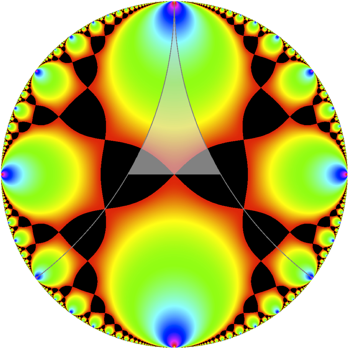
Figure 1: The modular invariant $|j(\tau)|$ plotted across the upper half plane $\mathbb{H}$, where $\mathbb{H}$ is conformally mapped to the unit disk via $w=\frac{1+i\tau}{i+\tau}$, so that $\tau=+i\infty$ (weak coupling) lies at the top edge of the disk, $\tau=i$ (intermediate coupling) in the center and $\tau=0$ (strong coupling) at the bottom, whereas the left and right edges correspond to $\tau=-1$ and $\tau=+1$ respectively, and the $\mathrm{Im\ }\tau=0$ axis spans the perimeter. The black regions, corresponding to $|j(\tau)|<12^{3}$, serve to divide the plane into an infinite number of disjoint colored regions, each containing a subregion with a weakly coupled dual description ($|j(\tau)|\to\infty$), colored blue/purple. The superimposed curved grey lines illustrate the boundary of the region $|\mathrm{Re\ }\tau|<1/2$, a fundamental domain under the identification $\tau\to\tau+1$. The transformation $\tau\to-1/\tau$ is equivalent to inversion through the center of the disk, and the shaded triangular region is the canonical fundamental domain for $SL(2,\mathbb{Z})$.

For an $SU(N)$ gauge group, all the dual descriptions have the same perturbative gauge group. This is a consequence of the invariance of the D3 brane under $SL(2,\mathbb{Z})$. We now consider Montonen-Olive duality for $SO$ and $U\!Sp$ gauge groups. For an $SO(2k)$ gauge group, the duals likewise have the same gauge group; equivalently, the O3^- plane is $SL(2,\mathbb{Z})$ invariant Witten:1998xy . For an $SO(2k+1)$ gauge group, however, the dual descriptions have gauge group $U\!Sp(2k)$. In string theory, this corresponds to the fact that the ($\tau\to-1/\tau$) S-dual of the $\widetilde{\rm O3}^{-}$ — another name for an O3^- plus a single (pinned) D3 brane — is an O3⁺. Thus, S-duality maps

$$\mathrm{O3}^{-}+(2k+1)\mbox{\ D3's}\longrightarrow\mathrm{O3}^{+}+2k\mbox{\ D3's}\,.$$ (3)

This is a well known example of what we will call an “orientifold transition”, wherein strongly coupled orientifold planes recombine with branes to form a different, weakly coupled orientifold plane. Examples of this phenomenon with collapsed O7 planes and $\mathcal{N}=1$ supersymmetry are considered in transitions2 , and play an important role in the new dualities discussed in this paper.

The upshot of the previous paragraph is that Montonen-Olive duality relates strongly coupled $\mathcal{N}=4$ gauge theories with $SO(2k+1)$ and $U\!Sp(2k)$ gauge groups to each other. This is not the whole story, however. Because the O3⁺ and $\widetilde{\rm O3}^{-}$ are related by S-duality, they must form some $SL(2,\mathbb{Z})$ multiplet. However, the multiplet is as yet incomplete. To see this, consider the $SL(2,\mathbb{Z})$ generators $T:\tau\to\tau+1$ and $S:\tau\to-1/\tau$. The $\widetilde{\rm O3}^{-}$ is $T$-invariant; therefore $ST$ maps $\widetilde{\rm O3}^{-}$ to O3⁺. However, since $(ST)^{3}=1$, it cannot be true that $ST$ maps O3⁺ back to $\widetilde{\rm O3}^{-}$. We denote the $ST$ image of O3⁺ as $\widetilde{\rm O3}^{+}$, where the three O3 planes form a triplet under $SL(2,\mathbb{Z})$ Witten:1998xy . We summarize the resulting structure in figure 2.

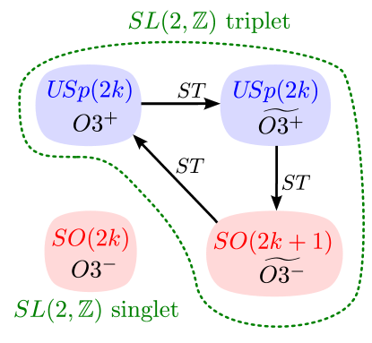
Figure 2: Summary of the four gauge theories that arise from placing D3 branes on top of the four different O3 planes.

The complete action of $SL(2,\mathbb{Z})$ on the triplet is as follows: $S$ exchanges the O3⁺ and $\widetilde{\rm O3}^{-}$, leaving the $\widetilde{\rm O3}^{+}$ invariant, whereas $T$ exchanges the O3⁺ and $\widetilde{\rm O3}^{+}$, leaving the $\widetilde{\rm O3}^{-}$ invariant, so that $ST$ cyclically permutes the three O3 planes. Since $T$ is a perturbative duality, the $\widetilde{\rm O3}^{+}$ also gives rise to an $U\!Sp(2k)$ gauge group, and is perturbatively equivalent to the O3⁺, the two configurations being distinguished non-perturbatively by their spectrum of BPS states Hanany:2000fq . It is possible to rephrase this by saying that the two different O3⁺ planes give rise to the same gauge theory at different theta angles. In particular, $\tau\to\tau+2$ leaves the O3 plane type invariant, and defines the periodicity of the theta angle in the corresponding gauge theory, whereas $\tau\to\tau+1$ exchanges the two O3 plane types. Thus, the gauge theories corresponding to $2k$ D3 branes atop an O3⁺ and $\widetilde{\rm O3}^{+}$ can be identified with each other upon shifting the theta angle by a half period.

To illustrate the nature of these dualities, we show how the weakly coupled description changes as a function of the holomorphic gauge coupling in figure 3. As can be seen in the figure, each gauge theory has additional self-dualities as well as the dualities which relate the different theories. For example, the self-duality group for $SO(2k+1)$ is the subgroup $\Gamma_{0}(2)\subset SL(2,\mathbb{Z})$ of elements $\bigl{(}\begin{smallmatrix}a&b\\ c&d\end{smallmatrix}\bigr{)}$ for which $c$ is even (hence $a$ and $d$ are odd, since $ad-bc=1$), whereas for $U\!Sp(2k)$ it is the conjugate subgroup consisting of elements for which $b$ is even.

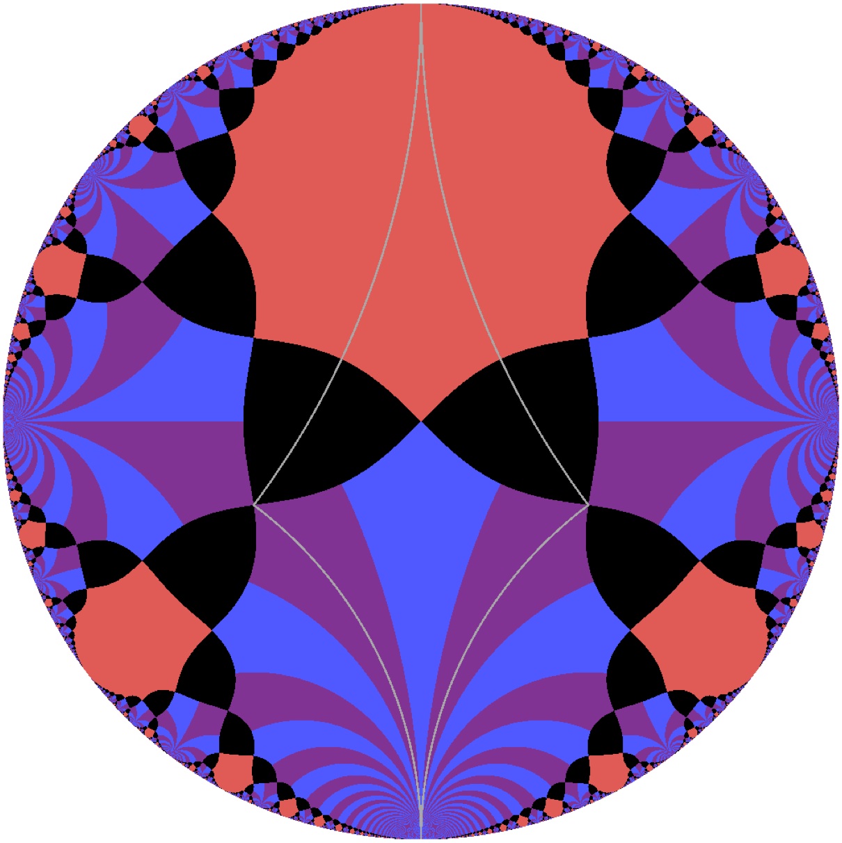
Figure 3: A schematic illustration of the phase structure of $\mathcal{N}=4$ $SO(2k+1)$ and $U\!Sp(2k)$ gauge theories as a function of $\tau$, patterned after figure 1. The different colors indicate the type of the O3 plane (and hence the gauge group) in the dual weakly coupled phase for each value of $\tau$, where red, blue and purple correspond to an $\widetilde{\rm O3}^{-}$, O3⁺ or $\widetilde{\rm O3}^{+}$, respectively, and the latter two possibilities are distinguished by requiring $-1/2<\mathrm{Re\ }\tau\leq 1/2$ in the dual theory. Thus, the red regions have a dual weakly coupled $SO(2k+1)$ description, whereas the blue/purple striped regions have a dual weakly coupled $U\!Sp(2k)$ description. The thin grey lines outline a fundamental region for $\Gamma_{0}(2)$, the self-duality group for the $SO(2k+1)$ theory. Note that the region where each dual theory is perturbative is most likely smaller than the colored region indicated here (see figure 1).

3 Duality for $\mathbb{C}^{3}/\mathbb{Z}_{3}$

In this section, we examine the simplest of our new $\mathcal{N}=1$ dualities. In the $\mathcal{N}=4$ examples discussed above, the six directions transverse to the D3 branes form a flat $\mathbb{R}^{6}$ or equivalently $\mathbb{C}^{3}$ transverse space, leading to gauge theories with maximal supersymmetry, where the $SU(4)\cong SO(6)$ R-symmetry is just the rotational isometry group of $\mathbb{R}^{6}$. To obtain an $\mathcal{N}=1$ theory at low energies, we must either switch on flux or introduce singularities. We choose to do the latter.

A simple and well-known example of such a transverse space is the $\mathbb{C}^{3}/\mathbb{Z}_{3}$ orbifold, where the orbifold action on the transverse complex coordinates is

$$z^{i}\to e^{2\pi i/3}z^{i}\,.$$ (4)

The singularity can be resolved by blowing up a $\mathbb{P}^{2}$ exceptional divisor. Placing D3 branes at the singularity leads to the $\mathcal{N}=1$ $SU(N)^{3}$ quiver gauge theory shown in figure 4. The orbifold reduces the isometry of the transverse space to $SU(3)\times U(1)$, with the $U(1)$ appearing as an R-symmetry in the $\mathcal{N}=1$ gauge theory.

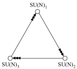
Figure 4: The quiver gauge theory for $\mathbb{C}^{3}/\mathbb{Z}_{3}$.

We consider an orientifold of this configuration, since, as we argued in the previous section, the $SL(2,\mathbb{Z})$ dual descriptions of gauge theories arising from D3 branes at singularities all have the same gauge group and matter content. We choose the orientifold involution $z^{i}\to-z^{i}$ which corresponds to an O7 plane wrapping the shrunken $\mathbb{P}^{2}$. As the resulting configuration is essentially a $\mathbb{Z}_{3}$ orbifold of the $\mathcal{N}=4$ orientifolds considered in the previous section, we will argue that the strong coupling behavior is closely analogous. In this paper we focus on the characteristics of the resulting gauge theories, deferring a detailed discussion of the analogy between the gravity duals to transitions2 .

In appendix A we discuss in general how to “orientifold” a quiver gauge theory and apply this procedure to two explicit examples. In particular in §A.2.2 we study the orientifolds of the $\mathbb{C}^{3}/\mathbb{Z}_{3}$ orbifold theory for the orientifold involution $z^{i}\to-z^{i}$. Counting $SO(2N)$ and $SO(2N+1)$ as two separate cases, we find that there are three possible gauge theories arising on D3 branes probing this orientifolded singularity. They correspond to a shrunken $\mathbb{P}^{2}$ that is wrapped by an O7⁺ plane or to an O7^- plane with and without a pinned D3 brane respectively.

We will argue that two of these gauge theories are dual, whereas the third is self-dual, analogous to the $\mathcal{N}=4$ $SO(2k+1)$, $U\!Sp(2k)$ and $SO(2k)$ gauge theories discussed above. The dualities studied here are merely the simplest examples of a large class of $\mathcal{N}=1$ dualities between orientifold gauge theories, some of which we will study in detail in this paper as well as in transitions2 ; transitions3 , where we will discuss many more examples.

The $\mathbb{C}^{3}/\mathbb{Z}_{3}$ orientifold we discuss here was, to the best of our knowledge, first studied in Angelantonj:1996uy ; Lykken:1997gy ; Lykken:1997ub ; Kakushadze:1998tr and recently revisited from the dimer point of view in Franco:2007ii ; Franco:2010jv and applied to the problem of moduli stabilization in Heidenreich:2010ad ; Cicoli:2012vw . Orientifolds of $\mathbb{C}^{3}/\mathbb{Z}_{3}$ and related abelian orbifolds have also proven to be an interesting testing ground for studying non-perturbative dynamics in string theory Bianchi:2007fx ; Bianchi:2007wy ; Bianchi:2009bg ; Bianchi:2009ij ; Bianchi:2012ud . For the involution discussed above, one finds $SO(N-4)\times SU(N)$ and $U\!Sp(\tilde{N}+4)\times SU(\tilde{N})$ gauge theories for collapsed O7^- and O7⁺ planes, respectively. Both theories have a non-anomalous R-symmetry in addition to a global $SU(3)$ symmetry, corresponding to the $SU(3)\times U(1)$ isometry of the transverse space. A careful analysis reveals that both models also have a discrete “baryonic” $\mathbb{Z}_{3}$ symmetry. The two models are

$$SO(N-4)$$

(14)

$$U\!Sp(\tilde{N}+4)$$

(23)

where $\omega_{n}\equiv e^{2\pi i/n}$, $\tilde{N}$ is even, and the tree-level superpotentials are

$$W=\frac{\lambda}{2}\epsilon_{ijk}\mathrm{Tr\,}A^{i}A^{j}B^{k}\,,\quad\tilde{W}=\frac{\tilde{\lambda}}{2}\epsilon_{ijk}\mathrm{Tr\,}\tilde{A}^{i}\tilde{A}^{j}\tilde{B}^{k}\,,$$ (24)

respectively, where $\lambda$ and $\tilde{\lambda}$ are superpotential couplings.

Note that we label the discrete symmetry as a $\mathbb{Z}_{3}$ even though the cube of the generator is not the identity. This is because the cube of the generator lies within the $\mathbb{Z}_{N}$ or $\mathbb{Z}_{\tilde{N}}$ center of $SU(N)$ or $SU(\tilde{N})$, so we obtain a $\mathbb{Z}_{3}$ symmetry upon composing the generator with an element of $SU(N)$ or $SU(\tilde{N})$ whose cube is the inverse of the cube of the generator. This latter $\mathbb{Z}_{3}$ symmetry is equivalent to the discrete symmetry indicated in the charge table up to a constant gauge transformation.

The $SO(N-4)\times SU(N)$ gauge theories have a classical moduli space which includes directions corresponding to moving D3 branes away from the singularity. The gauge group is then Higgsed down to $SO(N-4-2k)\times SU(N-2k)\times U(k)$ where $k$ is the number of (downstairs) D3 branes removed from the O-plane, corresponding to the $U(k)$ factor in the Higgsed gauge group. After integrating out massive matter, the $U(k)$ decouples from the rest of the gauge group in the IR, giving a separate $\mathcal{N}=4$ gauge theory corresponding to $k$ D3 branes probing a smooth region of the Calabi-Yau cone. Meanwhile, the remaining $SO(N-4-2k)\times SU(N-2k)$ reproduces the original gauge theory at a different rank $N^{\prime}=N-2k$. Thus, we see that the moduli space of the $SO(N-4)\times SU(N)$ family of gauge theories falls into two disconnected components for even and odd $N$ respectively, where all even $N$ theories are connected by the above process, as are all odd $N$ theories. Similarly, all $U\!Sp(\tilde{N}+4)\times SU(\tilde{N})$ theories are interconnected by an analogous motion in moduli space, where $\tilde{N}$ must be even for $U\!Sp(\tilde{N}+4)$ to exist.

In all, we have obtained three distinct families of gauge theories corresponding to D3 branes probing the orientifolded $\mathbb{C}^{3}/\mathbb{Z}_{3}$ singularity, all corresponding to the same geometric orientifold involution. Two of these theories, the $SO(N-4)\times SU(N)$ theories for even and odd $N$, are distinguished from each other by the presence or absence of a pinned D3 brane and its corresponding half-integral D3 brane charge, while the $U\!Sp(\tilde{N}+4)\times SU(\tilde{N})$ theory corresponds to a compact O7⁺ plane rather than a compact O7^- plane. Regardless of the O-plane type, the seven-brane tadpole is cancelled locally by (anti-)D7 branes, and the two configurations have the same $SL(2,\mathbb{Z})$ monodromy.

The situation is closely analogous to the three gauge theories $SO(2k)$, $SO(2k+1)$, $U\!Sp(2k)$ appearing in the $\mathcal{N}=4$ case, and we therefore hypothesize that one of the $SO$ families enjoys an $SL(2,\mathbb{Z})$ self-duality, whereas the other $SO$ family and the $U\!Sp$ family are related by an $SL(2,\mathbb{Z})$ duality. In the remainder of this section and in §4, we present strong field theoretic evidence for the latter duality, based on the matching of various computable infrared observables, and explore some of its properties.

We begin by discussing ’t Hooft anomaly matching in §3.1, leading to a more precise statement of the proposed duality. We then provide further evidence for the duality by a partial matching between the moduli spaces of the two theories. In §3.2, we highlight an important limitation of our methods which is nonetheless linked to the nature of the duality, and in §3.3 we discuss a specific, finite $N$ example of the proposed duality.

We continue our discussion of these gauge theories in the following sections. In §4, we provide further strong evidence for the proposed duality by comparing the superconformal indices between the prospectively dual theories, and in §5, we discuss their infrared physics using Seiberg duality.

3.1 Classic checks of the duality

As a precursor to anomaly matching, we note that the dual theories should have the same global symmetry groups. In particular, for $N$ or $\tilde{N}$ not divisible by three the baryonic $\mathbb{Z}_{3}$ is equivalent to the $\mathbb{Z}_{3}$ center of $SU(3)$ composed with a constant gauge transformation, and therefore lies within the continuous symmetry group, whereas for $N=0\mod\ 3$ the $\mathbb{Z}_{3}$ is distinct. Moreover, there is an additional $\mathbb{Z}_{2}$ “color conjugation” symmetry (see e.g. Csaki:1997aw ) for the $SO$ theory with even $N$, which comes from the outer automorphic group of $SO(2n)$. In net, the global symmetry group for the $SO$ theories is $SU(3)\times U(1)_{R}\times\mathbb{Z}_{\operatorname{gcf}(6,N)}$, whereas for the $U\!Sp$ theories it is $SU(3)\times U(1)_{R}\times\mathbb{Z}_{\operatorname{gcf}(3,\tilde{N})}$. Since the global symmetry groups must match between dual descriptions, this suggests that the ranks of the dual pair must be related as follows:

$$N=\tilde{N}+3k\,,$$ (25)

for some odd integer $k$ to be determined.

The global anomalies for the two models are shown in table 1.

$SO(N-4)\times SU(N)$ theory:		$U\!Sp(\tilde{N}+4)\times SU(\tilde{N})$ theory:
$SU(3)^{3}$ $\frac{3}{2}(N-3)N$ $SU(3)^{2}\,U(1)_{R}$ $-\frac{1}{2}(N-3)N-6$ $U(1)_{R}^{3}$ $\frac{4}{3}(N-3)N-33$ $U(1)_{R}$ $-9$ $SU(3)^{2}\,\mathbb{Z}_{3}$ 1 $\mathbb{Z}_{3}$ 1		$SU(3)^{3}$ $\frac{3}{2}\tilde{N}(\tilde{N}+3)$ $SU(3)^{2}\,U(1)_{R}$ $-\frac{1}{2}\tilde{N}(\tilde{N}+3)-6$ $U(1)_{R}^{3}$ $\frac{4}{3}\tilde{N}(\tilde{N}+3)-33$ $U(1)_{R}$ $-9$ $SU(3)^{2}\,\mathbb{Z}_{3}$ 1 $\mathbb{Z}_{3}$ 1

Table 1: The anomalies for the $\mathbb{C}^{3}/\mathbb{Z}_{3}$ orientifold gauge theories. In our notation, $G^{2}\mathbb{Z}_{k}=\prod_{i}\eta_{i}^{2T(r_{i})}$ and $(\mathrm{grav})^{2}\mathbb{Z}_{k}=\prod_{i}\eta_{i}^{2}$, where $\eta_{i}$ is the multiplicative charge of $i$th Weyl fermion under the generator of the $\mathbb{Z}_{k}$ discrete symmetry. For a discrete anomaly $\eta$, the Jacobian for the symmetry transformation in the path integral is $\eta^{n}$, where $n$ is the instanton number for the background in question; therefore, the anomaly vanishes iff $\eta=1$.

We see that the anomalies match between the two theories for $N=\tilde{N}+3$, in agreement with the restriction from matching the global symmetry groups discussed above. In transitions2 , it is shown that this rank relation agrees with D3 charge conservation, as it must. Since $\tilde{N}$ is necessarily even, this is evidence for a possible duality between the $SO(N-4)\times SU(N)$ theory for odd $N$ and the $U\!Sp(N+1)\times SU(N-3)$ theory. It will also follow from the arguments of transitions2 that the $SO(N-4)\times SU(N)$ theory for even $N$ is self-dual.

We now consider the moduli spaces of the prospectively dual theories, which is classically equivalent to the affine variety parameterized by the holomorphic gauge invariant operators identified under the F-term conditions and classical constraints Luty:1995sd . In general, a holomorphic gauge invariant of the $SO(N-4)\times SU(N)$ theory takes the form

$$\mathcal{O}^{N_{A},N_{B}}=A^{N_{A}}B^{N_{B}}\,,$$ (26)

for some particular choice of contraction of the gauge indices. Such operators may be classified as “mesons” or “baryons”, depending on whether the $SU(N)$ Levi-Civita symbol is irreducibly involved in the contraction of gauge indices or not, i.e. on whether the baryonic charge

$$Q_{A}\equiv(N_{A}-2N_{B})/N$$ (27)

is vanishing or not. The corresponding $U(1)_{A}$ is anomalous, with an anomaly-free $\mathbb{Z}_{3}$ subgroup that was identified above:

$$Q_{3}=\omega_{3}^{Q_{A}}\,,$$ (28)

where the $Q_{A}$ charge of a gauge invariant operator is necessary integral, since $\mathbb{Z}_{N}\subset SU(N)$ lies within the gauge group.

No $SO(N-4)$ gauge invariants exist for the case $N_{A}=1$ with $N>5$. Thus, baryonic operators can be further subdivided into those with $Q_{A}>0$, which can be “factored” as

$$\mathcal{O}=(A^{N})^{n_{1}}(AAB)^{n_{2}}\,,$$ (29)

and those with $Q_{A}<0$, which can be “factored” as

$$\mathcal{O}=(B^{N})^{n_{1}}(AAB)^{n_{2}}\,,$$ (30)

for integral powers $n_{1}$ and $n_{2}$.

We will focus on the “irreducible” baryons, of the form $\mathcal{O}_{k}^{(A)}\equiv A^{kN}$ and $\mathcal{O}_{k}^{(B)}=B^{kN}$. These have $R$-charges

$$Q_{R}(A^{kN})=\frac{2(N+3)}{3}k\,,\quad Q_{R}(B^{kN})=\frac{2(N-6)}{3}k\,,$$ (31)

and in both cases the $\mathbb{Z}_{3}$ charge $\omega_{3}^{k}$. “Reducible” baryons are similar, but with an additional $R$-charge of $+2$ for every factor of $(AAB)$ which appears.

The holomorphic gauge invariants of the $U\!Sp(\tilde{N}+4)\times SU(\tilde{N})$ theory can be similarly classified, where now the irreducible baryons have $R$-charges

$$Q_{R}(\tilde{A}^{k\tilde{N}})=\frac{2(\tilde{N}-3)}{3}k\,,\quad Q_{R}(\tilde{B}^{k\tilde{N}})=\frac{2(\tilde{N}+6)}{3}k\,,$$ (32)

with the $\mathbb{Z}_{3}$ charge $\omega_{3}^{k}$, as before.

In general, mesons and reducible and irreducible baryons can all be intermixed in the duality relations between the two theories. However, in certain cases only one type of operator with the correct $R$-charge exists. In particular, this occurs in the following cases for the $SO(N-4)\times SU(N)$ theory:

1. For $Q_{R}<2(N-6)$ and $Q_{3}=\omega_{3}^{0}$, only mesonic operators are possible.

2. For $Q_{3}=\omega_{3}$ and $Q_{3}=\omega_{3}^{-1}$, the minimum possible $R$-charges are $\frac{2(N-6)}{3}$ and $\frac{4(N-6)}{3}$, respectively, corresponding to the irreducible baryons $B^{N}$ and $B^{2N}$.

Similarly, for the $U\!Sp(\tilde{N}+4)\times SU(\tilde{N})$ theory:

1. For $Q_{R}<2(\tilde{N}-3)$ and $Q_{3}=\omega_{3}^{0}$, only mesonic operators are possible.

2. For $Q_{3}=\omega_{3}$ and $Q_{3}=\omega_{3}^{-1}$, the minimum possible $R$-charges are $\frac{2(\tilde{N}-3)}{3}$ and $\frac{4(\tilde{N}-3)}{3}$, respectively, corresponding to the irreducible baryons $\tilde{A}^{\tilde{N}}$ and $\tilde{A}^{2\tilde{N}}$.

This suggests the matching:

$$B^{N}\longleftrightarrow\tilde{A}^{\tilde{N}}\,,\quad B^{2N}\longleftrightarrow\tilde{A}^{2\tilde{N}}\,,$$ (33)

between the $Q_{3}=\omega_{3}$ and $Q_{3}=\omega_{3}^{-1}$ operators of minimum possible $R$-charge in both theories. In particular, these operators must have the same $R$-charge, i.e.

$$\frac{2(N-6)}{3}=\frac{2(\tilde{N}-3)}{3}\,,$$ (34)

which reproduces the rank relation $N=\tilde{N}+3$ that we saw from the anomaly matching conditions.

The $SU(3)$ representations of these operators should also match. For $\tilde{A}^{\tilde{N}}$, the $SU(3)$ representation can be determined as follows: the symplectic invariant contracts the $\tilde{A}$’s in pairs, and the operator therefore factors as $(\tilde{A}^{2})^{\tilde{N}/2}$. The $\tilde{B}$ F-term condition implies that the nonvanishing component of the $U\!Sp(\tilde{N}+4)$ invariant $\tilde{A}^{2}$ transforms as $(\overline{\leavevmode\hbox{\vtop{\offinterlineskip\openup-0.4pt\halign{&\startbox@YT{\defarg@YT}{}#\endbox@YT\cr\framebox{\vbox to5.0pt{\vss\hbox to5.0pt{\hss$$\hss}\vss}}\cr\framebox{\vbox to5.0pt{\vss\hbox to5.0pt{\hss$$\hss}\vss}}\cr}}\kern 5.0pt}},\leavevmode\hbox{\vtop{\offinterlineskip\openup-0.4pt\halign{&\startbox@YT{\defarg@YT}{}#\endbox@YT\cr\framebox{\vbox to5.0pt{\vss\hbox to5.0pt{\hss$$\hss}\vss}}&\framebox{\vbox to5.0pt{\vss\hbox to5.0pt{\hss$$\hss}\vss}}\cr}}\kern 10.0pt})_{4/3-4/\tilde{N}}$ under $SU(\tilde{N})\times SU(3)\times U(1)_{R}$. Thus, $\tilde{A}^{\tilde{N}}=(\tilde{A}^{2})^{\tilde{N}/2}$ takes the form of a “Pfaffian” of $\tilde{A}^{2}$, which is symmetric in its factors. The nonvanishing gauge-invariant component of $\tilde{A}^{\tilde{N}}$ therefore transforms in the $SU(3)$ representation

$$\operatorname{Sym}^{\tilde{N}/2}(\leavevmode\hbox{\vtop{\offinterlineskip\openup-0.4pt\halign{&\startbox@YT{\defarg@YT}{}#\endbox@YT\cr\framebox{\vbox to5.0pt{\vss\hbox to5.0pt{\hss$$\hss}\vss}}&\framebox{\vbox to5.0pt{\vss\hbox to5.0pt{\hss$$\hss}\vss}}\cr}}\kern 10.0pt})\equiv\underbrace{\leavevmode\hbox{\vtop{\offinterlineskip\openup-0.4pt\halign{&\startbox@YT{\defarg@YT}{}#\endbox@YT\cr\framebox{\vbox to5.0pt{\vss\hbox to5.0pt{\hss$$\hss}\vss}}&\framebox{\vbox to5.0pt{\vss\hbox to5.0pt{\hss$$\hss}\vss}}\cr}}\kern 10.0pt}\otimes_{S}\leavevmode\hbox{\vtop{\offinterlineskip\openup-0.4pt\halign{&\startbox@YT{\defarg@YT}{}#\endbox@YT\cr\framebox{\vbox to5.0pt{\vss\hbox to5.0pt{\hss$$\hss}\vss}}&\framebox{\vbox to5.0pt{\vss\hbox to5.0pt{\hss$$\hss}\vss}}\cr}}\kern 10.0pt}\otimes_{S}\ldots\otimes_{S}\leavevmode\hbox{\vtop{\offinterlineskip\openup-0.4pt\halign{&\startbox@YT{\defarg@YT}{}#\endbox@YT\cr\framebox{\vbox to5.0pt{\vss\hbox to5.0pt{\hss$$\hss}\vss}}&\framebox{\vbox to5.0pt{\vss\hbox to5.0pt{\hss$$\hss}\vss}}\cr}}\kern 10.0pt}}_{\tilde{N}/2}\,\,,$$ (35)

where $\otimes_{S}$ denotes the symmetric tensor product.

For $B^{N}$, the F-term conditions impose no additional constraints. Using the computer algebra package LiE LiE , one can show that the gauge invariant component of $B^{N}$ also transforms in $\operatorname{Sym}^{\tilde{N}/2}(\leavevmode\hbox{\vtop{\offinterlineskip\openup-0.4pt\halign{&\startbox@YT{\defarg@YT}{}#\endbox@YT\cr\framebox{\vbox to5.0pt{\vss\hbox to5.0pt{\hss$$\hss}\vss}}&\framebox{\vbox to5.0pt{\vss\hbox to5.0pt{\hss$$\hss}\vss}}\cr}}\kern 10.0pt})$ for $N=5,7,9,11$ and $13$ and $\tilde{N}=N-3$, whereas checking that this holds for larger $N$ is too computationally expensive using LiE directly. Using the more efficient approach explained in appendix E.1 we have verified agreement up to $N=21$. It would be desirable to have an argument for all $N$, and while we do not have a general proof, in appendix F we show how agreement between the $SU(3)$ representations of $\tilde{A}^{\tilde{N}}$ and $B^{N}$ follows from a certain conjectural mathematical identity involving representations of the symmetric group, and we provide additional evidence for this identity.

As a further check, we should be able to match the mesonic operators with $Q_{R}<2(N-6)=2(\tilde{N}-3)$ between the two theories. Such operators can be factored into products of single-trace operators of the form:

$$\mathcal{O}_{n}^{i_{1}j_{1}k_{1}\ldots i_{n}j_{n}k_{n}}\equiv\mathrm{Tr\,}(A^{i_{1}})^{T}B^{j_{1}}A^{k_{1}}\ldots(A^{i_{n}})^{T}B^{j_{n}}A^{k_{n}}\,,$$ (36)

where the F-term conditions imply that $\mathcal{O}_{n}$, with $Q_{R}=2n$, is totally symmetric in its $3n$ $SU(3)$ indices. A similar argument goes through for the $U\!Sp(\tilde{N}+4)\times SU(\tilde{N})$ theory, resulting in the same spectrum of single-trace operators.

3.2 Limitations from the perturbativity of the string coupling

Before turning to specific examples of the duality, we briefly review some general obstructions to having a perturbative description of the D-brane gauge theories obtained from quantization of open strings. For a “perturbative description”, we require that there exists some energy scale at which the gauge theory is weakly coupled, rather than weak coupling in the infrared. The nature of these obstructions will also serve to illustrate how our proposed duality differs from Seiberg duality.

The one-loop beta function for a supersymmetric gauge theory is given by Terning:2006bq :

$$\beta(g)\equiv\frac{dg}{d\ln\mu}=-\frac{g^{3}}{16\pi^{2}}\left(3\,T(\text{Adj})-\sum_{i}T(r_{i})\right)\,,$$ (37)

where $T(r)$ denotes the Dynkin index for the representation $r$, Adj denotes the adjoint representation, and the sum is taken over all chiral superfields. If $g$ is taken to be the holomorphic gauge coupling, then this result is exact, whereas the corresponding exact result for the physical gauge coupling depends on the anomalous dimensions of the chiral superfields.

The one-loop beta function coefficients (the term within parentheses in (37)) for the gauge group factors of the $SO$ theory are:

$$b_{SO}=-18\,,\quad b_{SU}=9\,,$$ (38)

whereas for those of the $U\!Sp$ theory they are

$$\tilde{b}_{U\!Sp}=9\,,\quad\tilde{b}_{SU}=-9\,.$$ (39)

Since the beta functions for the two gauge group factors have opposite signs, neither gauge theory is either IR free or asymptotically free, and the perturbative description will be valid at most in a finite range of energy scales. More precisely, a perturbative description at any scale is only possible if there is a separation between the dynamical scales, $\Lambda_{SO}\gg\Lambda_{SU}$ or $\tilde{\Lambda}_{SU}\gg\tilde{\Lambda}_{U\!Sp}$, along with a small superpotential coupling ($\lambda\ll 1$ or $\tilde{\lambda}\ll 1$) somewhere between these two scales. We will work in this limit. While it is possible in principle to incorporate corrections which are subleading in an expansion in small $\Lambda_{SU}/\Lambda_{SO}$ or $\tilde{\Lambda}_{U\!Sp}/\tilde{\Lambda}_{SU}$, this can be very difficult in practice, and we will not attempt to do so.

Conversely, the duality we propose partly addresses the question of what happens to the gauge theory in the limit where the dynamical scales have an inverted hierarchy. To see why, note that the string coupling is given by

$$\tau_{\rm 10d}=\frac{1}{2\pi i}\ln\left[\lambda^{6(N-2)}\Lambda_{SO(N-4)}^{-18}\Lambda_{SU(N)}^{18}\right]\,,\quad\tau_{\rm 10d}=\frac{1}{\pi i}\ln\left[\tilde{\lambda}^{3(\tilde{N}+2)}\Lambda_{U\!Sp(\tilde{N}+4)}^{9}\Lambda_{SU(\tilde{N})}^{-9}\right],$$ (40)

for the prospective dual theories, up to a multiplicative numerical factor within the square brackets. This result can be established in a variety of ways; for completeness, we present a Coulomb branch computation of it in appendix D. The result is also intuitive: a perturbative gauge theory necessarily corresponds to a weak string coupling.

The duality we propose acts as a modular transformation on $\tau_{\rm 10d}$, mapping any perturbative string coupling to a nonperturbative one. Conversely, deforming to strong string coupling and applying the duality, we obtain a dual description with a weak string coupling. Thus, since the string coupling is linked to the hierarchy $\Lambda_{SU}/\Lambda_{SO}$ or $\tilde{\Lambda}_{U\!Sp}/\tilde{\Lambda}_{SU}$, the duality provides at least partial information about the behavior of these gauge theories with an inverted hierarchy $\Lambda_{SU}\gg\Lambda_{SO}$ or $\tilde{\Lambda}_{U\!Sp}\gg\tilde{\Lambda}_{SU}$.

By contrast, Seiberg duality is generally used to understand the infrared behavior of a gauge theory which is perturbative at some scale, an illustration of the different natures of these two types of duality. While we can repeatedly apply Seiberg duality (together with deconfinement) to the individual gauge group factors, in our experience such an exercise never reproduces the prospective dual gauge theory, providing further circumstantial evidence that the duality is not a Seiberg duality in the usual sense. Indeed, if we were able to do so, we would have to somehow reconcile the complicated gauge coupling relations which result from applying modular transformations to (40) with the algebraic relationships between dynamical scales predicted by Seiberg duality.

With these considerations in mind, we turn to a specific example of the proposed duality.

3.3 Case study: the $SU(5)\longleftrightarrow U\!Sp(6)\times SU(2)$ duality

Since we are constrained to $N\geq 4$ and $\tilde{N}\geq 0$ to have gauge groups of non-negative rank, the lowest rank duality we expect to find is between the $SU(5)$ and $U\!Sp(6)\times SU(2)$ gauge theories:

$$\mbox{ \begin{minipage}{156.10345pt} \begin{center} \begin{tabular}[]{c|c|cc}&$\!SU(5)\!$&$\!SU(3)\!\!\!$&$\!U(1)_{R}\!$\\ \hline\cr$\!A^{i}\!$&$\overline{\leavevmode\hbox{\vtop{\offinterlineskip\openup-0.4pt\halign{&\startbox@YT{\defarg@YT}{}#\endbox@YT\cr\framebox{\vbox to5.0pt{\vss\hbox to5.0pt{\hss$$\hss}\vss}}\cr}}\kern 5.0pt}}$ &$\leavevmode\hbox{\vtop{\offinterlineskip\openup-0.4pt\halign{&\startbox@YT{\defarg@YT}{}#\endbox@YT\cr\framebox{\vbox to5.0pt{\vss\hbox to5.0pt{\hss$$\hss}\vss}}\cr}}\kern 5.0pt}$ &$16/15$\\ $\!B^{i}\!$&$\leavevmode\hbox{\vtop{\offinterlineskip\openup-0.4pt\halign{&\startbox@YT{\defarg@YT}{}#\endbox@YT\cr\framebox{\vbox to5.0pt{\vss\hbox to5.0pt{\hss$$\hss}\vss}}\cr\framebox{\vbox to5.0pt{\vss\hbox to5.0pt{\hss$$\hss}\vss}}\cr}}\kern 5.0pt}$ &\leavevmode\hbox{\vtop{\offinterlineskip\openup-0.4pt\halign{&\startbox@YT{\defarg@YT}{}#\endbox@YT\cr\framebox{\vbox to5.0pt{\vss\hbox to5.0pt{\hss$$\hss}\vss}}\cr}}\kern 5.0pt}&$-2/15$\end{tabular}\\ $W=\frac{1}{2}\lambda\,\epsilon_{ijk}A^{i}_{m}A^{j}_{n}B^{mn;\,k}$ \,, \end{center} \end{minipage}}\longleftrightarrow\mbox{\begin{minipage}{195.12767pt} \begin{center} \begin{tabular}[]{c|cc|cc}&$\!U\!Sp(6)\!\!$&$\!SU(2)\!$&$\!SU(3)\!\!\!$&$\!U(1)_{R}\!$\\ \hline\cr$\!\tilde{A}^{i}\!$&$\leavevmode\hbox{\vtop{\offinterlineskip\openup-0.4pt\halign{&\startbox@YT{\defarg@YT}{}#\endbox@YT\cr\framebox{\vbox to5.0pt{\vss\hbox to5.0pt{\hss$$\hss}\vss}}\cr}}\kern 5.0pt}$ &$\leavevmode\hbox{\vtop{\offinterlineskip\openup-0.4pt\halign{&\startbox@YT{\defarg@YT}{}#\endbox@YT\cr\framebox{\vbox to5.0pt{\vss\hbox to5.0pt{\hss$$\hss}\vss}}\cr}}\kern 5.0pt}$ &$\leavevmode\hbox{\vtop{\offinterlineskip\openup-0.4pt\halign{&\startbox@YT{\defarg@YT}{}#\endbox@YT\cr\framebox{\vbox to5.0pt{\vss\hbox to5.0pt{\hss$$\hss}\vss}}\cr}}\kern 5.0pt}$ &$-1/3$\\ $\!\tilde{B}^{i}\!$&$\mathbf{1}$&$\leavevmode\hbox{\vtop{\offinterlineskip\openup-0.4pt\halign{&\startbox@YT{\defarg@YT}{}#\endbox@YT\cr\framebox{\vbox to5.0pt{\vss\hbox to5.0pt{\hss$$\hss}\vss}}&\framebox{\vbox to5.0pt{\vss\hbox to5.0pt{\hss$$\hss}\vss}}\cr}}\kern 10.0pt}$ &\leavevmode\hbox{\vtop{\offinterlineskip\openup-0.4pt\halign{&\startbox@YT{\defarg@YT}{}#\endbox@YT\cr\framebox{\vbox to5.0pt{\vss\hbox to5.0pt{\hss$$\hss}\vss}}\cr}}\kern 5.0pt}&$8/3$\end{tabular}\\ $W=\frac{1}{2}\tilde{\lambda}\,\Omega^{ab}\epsilon_{ijk}\tilde{A}^{i}_{a;\,m}\tilde{A}^{j}_{b;\,n}\tilde{B}^{mn;\,k}$ \,, \end{center} \end{minipage}}$$ (41)

where $\Omega$ denotes the symplectic invariant. We characterize the classical moduli space of both theories, and show that both generate a runaway superpotential.

We discuss higher rank examples in §5.

3.3.1 The $U\!Sp(6)\times SU(2)$ theory

The F-term conditions are

$$\Omega^{ab}\tilde{A}^{[i}_{a;\,m}\tilde{A}^{j]}_{b;\,n}=0\,,\quad\tilde{A}^{[j}_{b;\,n}\tilde{B}^{k];\,mn}=0\,.$$ (42)

The first condition implies that all nonvanishing $U\!Sp(6)$ holomorphic gauge invariants are built from

$$\mathcal{A}^{ij}=\Omega^{ab}\epsilon^{mn}\tilde{A}^{i}_{a;\,m}\tilde{A}^{j}_{b;\,n}\,,$$ (43)

which transforms as a $\leavevmode\hbox{\vtop{\offinterlineskip\openup-0.4pt\halign{&\startbox@YT{\defarg@YT}{}#\endbox@YT\cr\framebox{\vbox to5.0pt{\vss\hbox to5.0pt{\hss$$\hss}\vss}}&\framebox{\vbox to5.0pt{\vss\hbox to5.0pt{\hss$$\hss}\vss}}\cr}}\kern 10.0pt}_{\,-2/3}$ under $SU(3)\times U(1)_{R}$. The remaining holomorphic gauge invariants are easily cataloged:

$$\mathcal{B}^{ij}=\epsilon_{mp}\epsilon_{nq}\tilde{B}^{i;\,mn}\tilde{B}^{j;\,pq}\,,\quad\mathcal{B}=\frac{1}{6}\epsilon_{ijk}\epsilon_{np}\epsilon_{qr}\epsilon_{sm}\tilde{B}^{i;\,mn}\tilde{B}^{j;\,pq}\tilde{B}^{k;\,rs}\,,$$ (44)

which transform as $\leavevmode\hbox{\vtop{\offinterlineskip\openup-0.4pt\halign{&\startbox@YT{\defarg@YT}{}#\endbox@YT\cr\framebox{\vbox to5.0pt{\vss\hbox to5.0pt{\hss$$\hss}\vss}}&\framebox{\vbox to5.0pt{\vss\hbox to5.0pt{\hss$$\hss}\vss}}\cr}}\kern 10.0pt}_{16/3}$ and $\mathbf{1}_{8}$, respectively, and obey the constraint $\mathcal{B}^{2}=\frac{1}{2}\det\mathcal{B}^{ij}$.

The second F-term condition implies a constraint relating $\mathcal{A}^{ij}$ and $\mathcal{B}^{ij}$. In particular,

$$\mathcal{A}^{ij}\mathcal{B}^{kl}=\Omega^{ab}\epsilon^{mn}\epsilon_{pr}\epsilon_{qs}\tilde{A}^{i}_{a;\,m}\tilde{A}^{j}_{b;\,n}\tilde{B}^{k;\,pq}\tilde{B}^{l;\,rs}=2\Omega^{ab}\epsilon_{qs}\tilde{A}^{i}_{a;\,m}\tilde{A}^{j}_{b;\,n}\tilde{B}^{k;\,mq}\tilde{B}^{l;\,ns}\,,$$ (45)

where we apply the first F-term condition to simplify the right-hand side. The second F-term condition then implies the constraint

$$\mathcal{A}^{i[j}\mathcal{B}^{k]l}=0\,.$$ (46)

Thus, the classical moduli space has three distinct branches:

1. A branch with $\mathcal{B}^{ij}=0$, parameterized by $\mathcal{A}^{ij}\neq 0$. For generic (full-rank) $\mathcal{A}^{ij}$, $U\!Sp(6)\times SU(2)$ breaks to a diagonal $SU(2)$, whereas for rank-deficient $\mathcal{A}^{ij}$, a larger gauge symmetry remains: $U\!Sp(4)\times SU(2)$ for $\mathcal{A}^{ij}$ rank one and $SU(2)\times SU(2)$ for $\mathcal{A}^{ij}$ rank two.

2. A branch with $\mathcal{A}^{ij}=0$, parameterized by $\mathcal{B}^{ij}\neq 0$ (and $\mathcal{B}$). For $\mathcal{B}^{ij}$ rank two or three, the $SU(2)$ gauge factor is completely broken, whereas $SU(2)\to U(1)$ for $\mathcal{B}^{ij}$ rank one.

3. A branch with $\mathcal{A}^{ij}=e^{i\phi}\cos\theta\,v^{i}v^{j}$ and $\mathcal{B}^{ij}=e^{-i\phi}\sin\theta\,v^{i}v^{j}$. $U\!Sp(6)\times SU(2)$ breaks to $U\!Sp(4)\times U(1)$, except for when $\theta=0$ or $\theta=\pi/2$, where this branch intersects branches 1 and 2, respectively.

We now discuss quantum corrections to this picture. The $U\!Sp(6)$ gauge factor is asymptotically free, whereas the $SU(2)$ gauge factor is infrared free. Thus, the infrared dynamics are primary governed by $U\!Sp(6)$ (to leading order in $\Lambda_{U\!Sp(6)}\ll\Lambda_{SU(2)}$), which generates an ADS superpotential:

$$W_{\rm ADS}=\frac{\Lambda_{\rm Sp}^{9}}{\det\tilde{A}}\,,$$ (47)

where $\tilde{A}$ is viewed as a $6\times 6$ matrix over $U\!Sp(6)\times(SU(2)\times SU(3))$.

We now consider the effect of the ADS superpotential on the moduli space. It is helpful to rewrite $\tilde{B}$ in the form:

$$\tilde{B}_{mn}^{i}=\frac{1}{2}\epsilon^{ijk}\hat{B}_{j_{m}k_{n}}\,,$$ (48)

where $\hat{B}$ transforms as $\overline{\leavevmode\hbox{\vtop{\offinterlineskip\openup-0.4pt\halign{&\startbox@YT{\defarg@YT}{}#\endbox@YT\cr\framebox{\vbox to5.0pt{\vss\hbox to5.0pt{\hss$$\hss}\vss}}\cr\framebox{\vbox to5.0pt{\vss\hbox to5.0pt{\hss$$\hss}\vss}}\cr}}\kern 5.0pt}}$ under a (fictitious) $SU(6)\supset SU(2)\times SU(3)$ flavor symmetry, which is broken by the constraint:

$$\epsilon^{mn}\hat{B}_{j_{m}k_{n}}=0\,,$$ (49)

as well as the (weak) gauging of $SU(2)$. We impose the constraint via a Lagrange multiplier field $M^{ij}$:

$$W=\frac{1}{2}\tilde{\lambda}\,\Omega^{ab}\tilde{A}_{a}^{M}\tilde{A}_{b}^{N}\hat{B}_{MN}+\frac{1}{2}\epsilon^{mn}\hat{B}_{i_{m}j_{n}}M^{ij}+\frac{\Lambda_{\rm Sp}^{9}}{\det\tilde{A}}\,,$$ (50)

where $M,N$ index the (fictitious) $SU(6)$. The $\hat{B}$ F-term condition is then

$$\tilde{\lambda}\,\Omega^{ab}\tilde{A}_{a}^{i_{m}}\tilde{A}_{b}^{j_{n}}=-\epsilon^{mn}M^{ij}\,,$$ (51)

so $M^{ij}$ is related to the holomorphic gauge invariant $\mathcal{A}^{ij}$. Finally, the $\tilde{A}$ F-term condition reads:

$$\tilde{\lambda}\,\Omega^{ab}\tilde{A}_{b}^{N}\hat{B}_{MN}=\frac{\Lambda_{\rm Sp}^{9}}{\det\tilde{A}}\,\left(\tilde{A}^{-1}\right)^{a}_{M}\,,$$ (52)

or

$$\hat{B}_{MN}=-\frac{\Lambda_{\rm Sp}^{9}}{\det\tilde{A}}\,\left[\left(\tilde{\lambda}\,\tilde{A}^{T}\Omega\tilde{A}\right)^{-1}\right]_{MN}\,.$$ (53)

Applying (51), we obtain

$$\hat{B}_{i_{m}j_{n}}=-\frac{\Lambda_{\rm Sp}^{9}}{\det\tilde{A}}\,\epsilon_{mn}\,M^{-1}_{ij}\,.$$ (54)

However, this is incompatible with the constraint (49). Therefore, supersymmetry is broken.

In particular, for generic $|\tilde{A}|\gg|\tilde{\lambda}^{-1/9}\Lambda_{\rm Sp}|$, the classical superpotential dominates, and the classical F-terms set $\tilde{B}=0$. We obtain a semiclassical “moduli-space” parameterized by $\mathcal{A}^{ij}$, subject to a runaway scalar potential generated by the ADS superpotential:

$$W_{\rm eff}\sim\frac{\Lambda_{\rm Sp}^{9}}{\det\mathcal{A}}\,.$$ (55)

3.3.2 The $SU(5)$ theory

The F-term conditions are:

$$A^{[i}_{a}A^{j]}_{b}=0\,,\quad A^{[j}_{a}B^{k];\,ab}=0\,.$$ (56)

We now characterize the classical moduli space. The first F-term constraint implies that

$$\langle A^{i}_{a}\rangle=v^{i}u_{a}\,,$$ (57)

where we may choose $u_{a}u^{*a}=1$ without loss of generality. Suppose that $\langle A^{i}_{a}\rangle\neq 0$. We gauge fix such that $u_{a}=(0,0,0,0,1)$. Thus, the second F-term constraint implies

$$\langle B^{i;\hat{a}5}\rangle=b^{\hat{a}}v^{i}\,,\quad B^{i;\hat{a}\hat{b}}=b^{i;\hat{a}\hat{b}}\,,$$ (58)

where $\hat{a},\hat{b}=1\ldots 4$.

Due to the first F-term constraint, the only possible nonvanishing holomorphic gauge invariant involving $A$ is the following:

$$\mathcal{O}^{ijkl}=A^{i}_{a}B^{j;\,ab}B^{k;\,cd}B^{l;\,ef}\epsilon_{bcdef}\,.$$ (59)

However, applying the above gauge-fixed forms for $\langle A\rangle$ and $\langle B\rangle$, we find that this also vanishes. This suggests that $\langle A\rangle=0$ once the D-term conditions are imposed, which can be verified by an explicit computation.

Since the F-term conditions are then identically satisfied, the classical moduli space is the subset of that of the $\lambda=0$ theory (without a superpotential) where $\langle A\rangle=0$. This theory is s-confining, with the confined description Csaki:1996sm ; Csaki:1996zb :

$$\begin{array}[]{c|c|cccc}&SU(5)&SU(3)&SU(3)&U(1)&U(1)_{R}\\ \hline\cr A^{i}&\overline{\leavevmode\hbox{\vtop{\offinterlineskip\openup-0.4pt\halign{&\startbox@YT{\defarg@YT}{}#\endbox@YT\cr\framebox{\vbox to5.0pt{\vss\hbox to5.0pt{\hss$$\hss}\vss}}\cr}}\kern 5.0pt}}&\leavevmode\hbox{\vtop{\offinterlineskip\openup-0.4pt\halign{&\startbox@YT{\defarg@YT}{}#\endbox@YT\cr\framebox{\vbox to5.0pt{\vss\hbox to5.0pt{\hss$$\hss}\vss}}\cr}}\kern 5.0pt}&\mathbf{1}&-3&16/15\\ B^{i}&\leavevmode\hbox{\vtop{\offinterlineskip\openup-0.4pt\halign{&\startbox@YT{\defarg@YT}{}#\endbox@YT\cr\framebox{\vbox to5.0pt{\vss\hbox to5.0pt{\hss$$\hss}\vss}}\cr\framebox{\vbox to5.0pt{\vss\hbox to5.0pt{\hss$$\hss}\vss}}\cr}}\kern 5.0pt}&\mathbf{1}&\leavevmode\hbox{\vtop{\offinterlineskip\openup-0.4pt\halign{&\startbox@YT{\defarg@YT}{}#\endbox@YT\cr\framebox{\vbox to5.0pt{\vss\hbox to5.0pt{\hss$$\hss}\vss}}\cr}}\kern 5.0pt}&1&-2/15\\ \hline\cr\hline\cr T_{i}^{m}=A^{2}B&&\overline{\leavevmode\hbox{\vtop{\offinterlineskip\openup-0.4pt\halign{&\startbox@YT{\defarg@YT}{}#\endbox@YT\cr\framebox{\vbox to5.0pt{\vss\hbox to5.0pt{\hss$$\hss}\vss}}\cr}}\kern 5.0pt}}&\leavevmode\hbox{\vtop{\offinterlineskip\openup-0.4pt\halign{&\startbox@YT{\defarg@YT}{}#\endbox@YT\cr\framebox{\vbox to5.0pt{\vss\hbox to5.0pt{\hss$$\hss}\vss}}\cr}}\kern 5.0pt}&-5&2\\ U^{i;m}_{\;\;n}=AB^{3}&&\leavevmode\hbox{\vtop{\offinterlineskip\openup-0.4pt\halign{&\startbox@YT{\defarg@YT}{}#\endbox@YT\cr\framebox{\vbox to5.0pt{\vss\hbox to5.0pt{\hss$$\hss}\vss}}\cr}}\kern 5.0pt}&\text{Adj}&0&2/3\\ V^{mn}=B^{5}&&\mathbf{1}&\leavevmode\hbox{\vtop{\offinterlineskip\openup-0.4pt\halign{&\startbox@YT{\defarg@YT}{}#\endbox@YT\cr\framebox{\vbox to5.0pt{\vss\hbox to5.0pt{\hss$$\hss}\vss}}&\framebox{\vbox to5.0pt{\vss\hbox to5.0pt{\hss$$\hss}\vss}}\cr}}\kern 10.0pt}&5&-2/3\end{array}$$ (60)

with the dynamical superpotential:

$$W=\frac{1}{\Lambda^{9}}\left(\epsilon_{mnp}\,T_{i}^{m}U^{i;n}_{\;\;q}V^{pq}-\frac{1}{3}\epsilon_{ijk}\,U^{i;m}_{\;\;p}U^{j;n}_{\;\;m}U^{k;p}_{\;\;n}\right)\,,$$ (61)

up to an overall multiplicative factor, where

$$T^{m}_{i} \equiv\frac{1}{2}\epsilon_{ijk}A^{j}_{a}A^{k}_{b}B^{ab;m}\,,\qquad U^{i;m}_{\;\;\;n}\equiv\frac{1}{12}\epsilon_{npq}\epsilon_{bcdef}A^{i}_{a}B^{ab;p}B^{cd;q}B^{ef;m}\,,$$

$$V^{mn} \equiv\frac{1}{160}\epsilon_{pqr}\epsilon_{a_{1}b_{1}c_{1}d_{1}e_{1}}\epsilon_{a_{2}b_{2}c_{2}d_{2}e_{2}}B^{a_{1}a_{2};p}B^{b_{1}c_{1};q}B^{b_{2}c_{2};r}B^{d_{1}e_{1};m}B^{d_{2}e_{2};n}\,.$$ (62)

One feature of s-confining theories is that their classical and quantum moduli spaces match. Thus, the above spectrum of gauge invariants describes the classical moduli space of the $\lambda=0$ theory, subject to the classical constraints, which are equivalent to the F-term conditions arising from the dynamical superpotential. Setting $\langle A\rangle=0$, we find $\langle T\rangle=\langle U\rangle=0$, with no remaining F-term constraints on $V$. Thus, the classical moduli space of the $\lambda\neq 0$ theory is parameterized by $V^{ij}$, which transforms as a $\leavevmode\hbox{\vtop{\offinterlineskip\openup-0.4pt\halign{&\startbox@YT{\defarg@YT}{}#\endbox@YT\cr\framebox{\vbox to5.0pt{\vss\hbox to5.0pt{\hss$$\hss}\vss}}&\framebox{\vbox to5.0pt{\vss\hbox to5.0pt{\hss$$\hss}\vss}}\cr}}\kern 10.0pt}_{\;-2/3}$ under the $SU(3)\times U(1)_{R}$ preserved by the superpotential. This matches branch 1 of the classical moduli space of the $U\!Sp(6)\times SU(2)$ theory described above, and both are parameterized by the baryon discussed in §3.1.

To obtain a quantum description of this theory, we perturb the s-confining theory (without superpotential) by the classical superpotential $AAB$, which can now be written in the form:

$$W_{\rm class}=\lambda T^{i}_{i}\,,$$

which breaks $SU(3)\times SU(3)\times U(1)\to SU(3)_{\rm diag}$, but preserves $U(1)_{R}$. One can show that the resulting F-term conditions cannot be solved, and therefore supersymmetry is broken Lykken:1998ec .

For simplicity, we restrict our attention to the case where $V^{ij}$ is full rank. We are then entitled to make the field redefinitions:

$$T^{i}_{j}=\hat{T}^{i}_{j}+\frac{\lambda^{2}\Lambda^{18}}{4\det V}\delta^{i}_{j}\,,\quad U^{ij}_{l}=\hat{U}^{ij}_{k}-\frac{1}{2}\lambda\,\Lambda^{9}\,\epsilon^{ijk}V^{-1}_{kl}\,.$$ (63)

The resulting superpotential is

$$W=\frac{1}{\Lambda^{9}}\,\epsilon_{ijk}\left(\hat{T}_{l}^{i}\hat{U}^{lj}_{m}V^{mk}+\frac{1}{3}\hat{U}^{il}_{n}\hat{U}^{jm}_{l}\hat{U}^{kn}_{m}\right)+\frac{\lambda}{2}\left(\hat{U}^{ik}_{l}\hat{U}^{lj}_{k}-\hat{U}^{ij}_{l}\hat{U}^{kl}_{k}\right)V^{-1}_{ij}+\frac{\lambda^{3}\Lambda^{18}}{4\det V}\,.$$ (64)

To show that there are no F-flat solutions, we first show that $\hat{T}=\hat{U}=0$ is the only solution to $\hat{T}$ and $\hat{U}$ F-term conditions for full-rank $V$. Note that in this case, $V^{ij}$ can always be brought to the form $V^{ij}\propto\delta^{ij}$ after a complexified $SU(3)$ transformation. As the F-term conditions are appropriately covariant under this complexified symmetry transformation, it is sufficient to show that $\hat{T}=\hat{U}=0$ is the only solution for $V^{ij}=z\,\delta^{ij}$.

In this case, the $\hat{T}$ F-term conditions reduce to

$$\epsilon_{ijk}\hat{U}^{lj}_{k}=0\,,$$ (65)

so that $\hat{U}^{ij}_{k}=\hat{U}^{ik}_{j}$. The $\hat{U}$ F-term conditions are:

$$0=\frac{1}{\Lambda^{9}}\,\left(\epsilon_{inm}\hat{T}_{k}^{i}\,z+\epsilon_{ijk}\hat{U}^{il}_{n}\hat{U}^{jm}_{l}\right)+\frac{\lambda}{2z}\left(\hat{U}^{mk}_{n}+\hat{U}^{nm}_{k}-\delta_{kn}\hat{U}^{im}_{i}-\delta_{km}\hat{U}^{ii}_{n}\right)\,.$$ (66)

Extracting the component which is symmetric in $n\leftrightarrow m$, we obtain

$$\hat{U}^{(nm)}_{k}-\delta_{k(n}\hat{U}^{ii}_{m)}=0$$ (67)

after applying the $T$ F-term condition. Contracting with $\delta_{km}$ we find $\hat{U}^{ii}_{j}=0$, so the above condition reduces to

$$\hat{U}^{mn}_{k}+\hat{U}^{nm}_{k}=0\,.$$ (68)

Together with the $\hat{T}$ F-term condition, this is sufficient to show that $\hat{U}=0$. The remaining components of the $\hat{U}$ F-term condition then imply that $\hat{T}=0$. By the above argument, these results apply for arbitrary (full-rank) $V$.

Having solved the $\hat{T}$ and $\hat{U}$ F-term conditions for $\hat{T}$ and $\hat{U}$, we may “integrate out” these fields, leaving the effective superpotential:

$$W_{\rm eff}=\frac{\lambda^{3}\Lambda^{18}}{4\det V}\,,$$ (69)

for $V^{ij}$, which has no F-flat solutions and generates a runaway scalar potential, much like the $U\!Sp(6)\times SU(2)$ theory.

4 Matching of superconformal indices

In this section we discuss another very nontrivial test of the proposed duality: the matching between the superconformal indices of the two gauge theories. The discussion is inherently somewhat technical in nature, and readers primarily interested in the gauge theoretic consequences of the proposed duality may wish to skip ahead to §5.

Superconformal indices for $\mathcal{N}=1$ theories compactified on $S^{3}\times\mathbb{R}$ Romelsberger:2005eg ; Kinney:2005ej , while being a relatively recent development, have already provided important insights into the topic of dualities. In particular, equality of the superconformal index provides very strong support for a number of known and conjectured Seiberg dualities between $\mathcal{N}=1$ theories Romelsberger:2007ec ; Dolan:2008qi ; Spiridonov:2008zr ; Spiridonov:2009za ; Spiridonov:2010hh ; Spiridonov:2011hf ; Sudano:2011aa ; Spiridonov:2012ww ; Yamazaki:2012cp ; Terashima:2012cx and S-dualities in $\mathcal{N}=2$ Gadde:2009kb ; Gadde:2010te ; Gadde:2011uv ; Gaiotto:2012uq and $\mathcal{N}=4$ theories Gadde:2009kb ; Spiridonov:2010qv . It also proves to be a very useful tool in the study of holography Kinney:2005ej . In this section we will present evidence for the agreement of the superconformal indices of the dual pair of theories presented in §3. As we will see momentarily, the agreement relies on extremely non-trivial group-theoretical identities, providing very strong support for our conjectured duality.

It is not our intention to give a detailed discussion of the superconformal index here (we refer the interested reader to Romelsberger:2005eg ; Kinney:2005ej ; Dolan:2008qi ; Sudano:2011aa for very readable expositions of the topic), but we will briefly review in this section the basic elements that enter into its computation in order to settle notation. Consider a four dimensional theory compactified on $S^{3}\times\mathbb{R}$. The superconformal algebra has generators $J_{\pm},J_{3},\overline{J}_{\pm},\overline{J}_{3}$ (associated to rotations on the $S^{3}$), supersymmetry generators $Q_{\alpha},\overline{Q}_{\dot{\alpha}}$, translations $P_{\mu}$, special superconformal generators $K_{\mu},S_{\alpha},\overline{S}_{\dot{\alpha}}$, superconformal dilatations $H$ and the $U(1)$ $R$-symmetry generator $R$. Define $Q=Q_{1}$, which implies Kinney:2005ej $Q^{\dagger}=S_{1}$. The superconformal algebra then gives:

$$2\{Q^{\dagger},Q\}=H-2J_{3}-\frac{3}{2}R\equiv\mathcal{H}\,.$$ (70)

The superconformal index is then defined by:

$$\mathrm{Tr\,}(-1)^{F}e^{-\beta\mathcal{H}}M\,,$$ (71)

with $F$ the fermion number operator, and $M$ any symmetry commuting with $Q$ and $Q^{\dagger}$. Let us choose $M$ to be generated by $\mathcal{R}\equiv R+2J_{3}$, $\overline{J}_{3}$, and gauge and flavor group elements $g,f$. Introducing appropriate chemical potentials, the refined index is thus given by:

$$\mathcal{I}(t,x,f)=\int\!dg\,\mathrm{Tr\,}(-1)^{F}e^{-\beta\mathcal{H}}t^{\mathcal{R}}x^{2\overline{J}_{3}}fg\,,$$ (72)

where we have integrated over the gauge group in order to count singlets only (we will have more to say about this integration below). It was argued in Kinney:2005ej that, exactly as in the case of the Witten index Witten:1982df , the index (72) receives contributions only from states annihilated by $Q$ and $Q^{\dagger}$, and thus the index does not actually depend on $\beta$, which plays the role of a regulator only.

In order to actually compute (72) we follow the prescription in Romelsberger:2007ec , which gives a systematic way of computing the superconformal index in terms of the fields in the weakly coupled Lagrangian description of the theory, when one is available. For a general weakly coupled theory $\mathcal{T}$ with gauge group $G$ and flavor group $F$, neither necessarily simple, and matter fields $X_{i}$ with superconformal $R$-charge $r_{i}$ in the representation $R^{i}_{G}\otimes R^{i}_{F}$ of $G\times F$, not necessarily irreducible, one constructs the letter

$$\begin{split}i_{\mathcal{T}}(t,x,g,f)&=\frac{(2t^{2}-t(x+x^{-1}))\chi_{\text{Adj}}(g)}{{(1-tx)(1-tx^{-1})}}\\ &\phantom{=}+\frac{\sum_{i}\left(t^{r_{i}}\chi_{R^{i}_{G}}(g)\,\chi_{R^{i}_{F}}(f)-t^{2-r_{i}}\chi_{\overline{R^{i}_{G}}}(g)\,\chi_{\overline{R^{i}_{F}}}(f)\right)}{(1-tx)(1-tx^{-1})}\,.\end{split}$$ (73)

Here $t,x,g,f$ are the same as in (72). $\chi_{R}(g)$ denotes the character of $g$ in the representation $R$, and we denote with bars the complex conjugate representations. Once we have the letter (73) for $\mathcal{T}$, the superconformal index $\mathcal{I}_{\mathcal{T}}$ is obtained by taking the plethystic exponential, and integrating over the gauge group:

$$\mathcal{I}_{\mathcal{T}}(t,x,f)=\int dg\,\exp\left[\,\sum_{k=1}^{\infty}\frac{1}{k}i_{\mathcal{T}}(t^{k},x^{k},g^{k},f^{k})\right]\,.$$ (74)

Here $dg$ denotes the Haar measure on the group $G$.

We will thus compute the index in a weakly coupled, non-conformal description of the theory, and will assume that this gives the right index for the theory at its (presumed) superconformal fixed point in the IR. In the case of the theory compactified on $S^{3}$, one can argue Gadde:2010en that since the index is independent of the radius $r$ of the $S^{3}$ it is independent of the dimensionless $r\Lambda$ coupling, and thus it is invariant under the RG flow and changes in the coupling constant. In order for this to be the case, we need to choose $M$ in (71) constant along the flow, and in particular it should agree with the value of $M$ at the IR superconformal fixed point. In particular, we need to choose the right value of the superconformal $R$-charge — determined using a-maximization Intriligator:2003jj , for instance — in constructing $M$.

Ideally, one would compute a closed form expression for (74) in the two dual phases, and then show that the two expressions agree for all $N$. Unfortunately we have not been able to prove the equality of the resulting indices, but in §4.1 and §4.2 we will provide very non-trivial evidence for the matching of the functions in two particularly tractable limits. The exact matching will thus remain a well motivated conjecture about elliptic hypergeometric integrals, which we formulate precisely in appendix G.

4.1 Expansion in $t$

The first limit corresponds to an expansion around $t=0$. Expanding (74) is elementary, but the integration over the gauge group requires some more advanced technology. In particular, one needs to use orthogonality of the characters under integration:

$$\int dg\,\chi_{R_{i}}(g)\chi_{\overline{R_{j}}}(g)=\delta_{ij}\,.$$ (75)

where $R_{i}$ and $R_{j}$ are irreps of $G$. When expanding the plethystic exponential (74) one encounters expressions of the form (we will deal with higher powers of $g$ momentarily):

$$\int dg\,\chi_{R_{1}}(g)\cdots\chi_{R_{n}}(g)\,.$$ (76)

By using the well know property of the characters $\chi_{R_{1}}(g)\chi_{R_{2}}(g)=\chi_{R_{1}\otimes R_{2}}(g)$, and then plugging the resulting expression into  (75) with the second term being the character of the trivial representation (i.e. just 1), we obtain that (76) just counts the number of singlets in $R_{1}\otimes\ldots\otimes R_{n}$.

When expanding (74) we will also encounter terms of the form $\chi_{R}(g^{n})$. The act of decomposing such terms into characters of irreducible representations with group element $g$ is known as applying the $n$-th Adams operator $\mathsf{A}_{n}$ to $R$. As an example, consider the fundamental representation for $SU(N)$, which has character:

$$\chi_{\scalebox{0.7}{$\leavevmode\hbox{\vtop{\offinterlineskip\openup-0.4pt\halign{&\startbox@YT{\defarg@YT}{}#\endbox@YT\cr\framebox{\vbox to3.5pt{\vss\hbox to3.5pt{\hss$$\hss}\vss}}\cr}}\kern 3.5pt}$}}(g)=\sum_{i=1}^{N}t_{i}\,$$

where $t_{i}$ are the elements of $g$ on the maximal torus of $SU(N)$. Similarly, for the symmetric and antisymmetric representations we have:

(82)

(85)

It is thus clear that $\mathsf{A}_{2}(\leavevmode\hbox{\vtop{\offinterlineskip\openup-0.4pt\halign{&\startbox@YT{\defarg@YT}{}#\endbox@YT\cr\framebox{\vbox to5.0pt{\vss\hbox to5.0pt{\hss$$\hss}\vss}}\cr}}\kern 5.0pt})=\leavevmode\hbox{\vtop{\offinterlineskip\openup-0.4pt\halign{&\startbox@YT{\defarg@YT}{}#\endbox@YT\cr\framebox{\vbox to5.0pt{\vss\hbox to5.0pt{\hss$$\hss}\vss}}&\framebox{\vbox to5.0pt{\vss\hbox to5.0pt{\hss$$\hss}\vss}}\cr}}\kern 10.0pt}-\leavevmode\hbox{\vtop{\offinterlineskip\openup-0.4pt\halign{&\startbox@YT{\defarg@YT}{}#\endbox@YT\cr\framebox{\vbox to5.0pt{\vss\hbox to5.0pt{\hss$$\hss}\vss}}\cr\framebox{\vbox to5.0pt{\vss\hbox to5.0pt{\hss$$\hss}\vss}}\cr}}\kern 5.0pt}$, or in terms of characters:

$$\chi_{\scalebox{0.7}{$\leavevmode\hbox{\vtop{\offinterlineskip\openup-0.4pt\halign{&\startbox@YT{\defarg@YT}{}#\endbox@YT\cr\framebox{\vbox to3.5pt{\vss\hbox to3.5pt{\hss$$\hss}\vss}}\cr}}\kern 3.5pt}$}}(g^{2})=\chi_{\scalebox{0.7}{$\leavevmode\hbox{\vtop{\offinterlineskip\openup-0.4pt\halign{&\startbox@YT{\defarg@YT}{}#\endbox@YT\cr\framebox{\vbox to3.5pt{\vss\hbox to3.5pt{\hss$$\hss}\vss}}&\framebox{\vbox to3.5pt{\vss\hbox to3.5pt{\hss$$\hss}\vss}}\cr}}\kern 7.0pt}$}}(g)-\chi_{\scalebox{0.7}{$\leavevmode\hbox{\vtop{\offinterlineskip\openup-0.4pt\halign{&\startbox@YT{\defarg@YT}{}#\endbox@YT\cr\framebox{\vbox to3.5pt{\vss\hbox to3.5pt{\hss$$\hss}\vss}}\cr\framebox{\vbox to3.5pt{\vss\hbox to3.5pt{\hss$$\hss}\vss}}\cr}}\kern 3.5pt}$}}(g)\,$$

Proceeding systematically in this way, one can decompose the plethystic exponential, up to any order, into sums of products of characters of irreps, which can then be easily integrated over the gauge group. The flavor characters can be dealt with similarly, and we will give the final results in terms of irreps. In the flavor case it is particularly important to do the decomposition into irreducible representations since there are important cancellations between terms, we will give an example below.

When the problem is formulated in this way the rest of the computation is conceptually straightforward, but doing this by hand quickly turns impossible, and the aid of computer systems is required for doing any non-trivial computations. We took advantage of the computer algebra package LiE LiE for doing the relevant group decompositions and Adams operations, and the mathematics software system Sage sage for the polynomial manipulations.

With this technology in place, the actual computation of the indices is straightforward, if lengthy. We obtain perfect agreement of the indices between the two dual theories in §3 up to the degrees that we checked. In particular, for $SO(3)\times SU(7)\leftrightarrow U\!Sp(8)\times SU(4)$, we obtain the index:

$$\mathcal{I}_{SO/U\!Sp}(t,x,f) =1+t^{\frac{2}{3}}\bigl{[}\chi_{0,2}(f)+\chi_{4,0}(f)\bigr{]}$$

$$\phantom{=}\,+t^{\frac{4}{3}}\bigl{[}2\chi_{0,4}(f)+2\chi_{2,0}(f)+\chi_{3,1}(f)+2\chi_{4,2}(f)+\chi_{8,0}(f)\bigr{]}$$

$$\phantom{=}\,+t^{\frac{5}{3}}(x+x^{-1})\bigl{[}\chi_{0,2}(f)+\chi_{4,0}(f)\bigr{]}$$

$$\phantom{=}\,+t^{2}\bigl{[}4+3\chi_{0,6}(f)+\chi_{1,4}(f)+5\chi_{2,2}(f)+3\chi_{3,3}(f)$$

$$\phantom{=\,+t^{2}\bigl{[}}+2\chi_{4,1}(f)+3\chi_{4,4}(f)+\chi_{5,2}(f)+4\chi_{6,0}(f)+\chi_{6,3}(f)$$

$$\phantom{=\,+t^{2}\bigl{[}}+\chi_{7,1}(f)+2\chi_{8,2}(f)+\chi_{12,0}(f)\bigr{]}+\ldots$$ (94)

where we have omitted terms of higher order in $t$. We have denoted the $SU(3)$ representation by its Dynkin labels, so for example the representation with $(2,2)$ Dynkin labels can be described as in terms of ordinary Young tableaux. Notice that, as we were indicating before, even at this relatively low order the matching of the indices is very non-trivial, with rather complicated character polynomials appearing. Furthermore, the agreement is only obtained after some rather involved group theory cancellations. As a particularly simple example, consider the $t^{\frac{2}{3}}$ term. In the $U\!Sp(8)\times SU(4)$ theory the relevant contribution after doing the gauge integration is of the form:

$$\mathcal{I}_{U\!Sp}(x,t,f)=t^{\frac{2}{3}}\biggl{[}\frac{1}{8}\chi_{\scalebox{0.7}{$\leavevmode\hbox{\vtop{\offinterlineskip\openup-0.4pt\halign{&\startbox@YT{\defarg@YT}{}#\endbox@YT\cr\framebox{\vbox to3.5pt{\vss\hbox to3.5pt{\hss$$\hss}\vss}}\cr}}\kern 3.5pt}$}}^{4}(f)+\frac{1}{4}\chi_{\scalebox{0.7}{$\leavevmode\hbox{\vtop{\offinterlineskip\openup-0.4pt\halign{&\startbox@YT{\defarg@YT}{}#\endbox@YT\cr\framebox{\vbox to3.5pt{\vss\hbox to3.5pt{\hss$$\hss}\vss}}\cr}}\kern 3.5pt}$}}^{2}(f)\chi_{\scalebox{0.7}{$\leavevmode\hbox{\vtop{\offinterlineskip\openup-0.4pt\halign{&\startbox@YT{\defarg@YT}{}#\endbox@YT\cr\framebox{\vbox to3.5pt{\vss\hbox to3.5pt{\hss$$\hss}\vss}}\cr}}\kern 3.5pt}$}}(f^{2})+\frac{3}{8}\chi_{\scalebox{0.7}{$\leavevmode\hbox{\vtop{\offinterlineskip\openup-0.4pt\halign{&\startbox@YT{\defarg@YT}{}#\endbox@YT\cr\framebox{\vbox to3.5pt{\vss\hbox to3.5pt{\hss$$\hss}\vss}}\cr}}\kern 3.5pt}$}}^{2}(f^{2})+\frac{1}{4}\chi_{\scalebox{0.7}{$\leavevmode\hbox{\vtop{\offinterlineskip\openup-0.4pt\halign{&\startbox@YT{\defarg@YT}{}#\endbox@YT\cr\framebox{\vbox to3.5pt{\vss\hbox to3.5pt{\hss$$\hss}\vss}}\cr}}\kern 3.5pt}$}}(f^{4})\biggr{]}+\ldots$$ (102)

where we have ignored terms of other orders in $t$. On the other hand, the corresponding expression for the $SO(3)\times SU(7)$ theory is given by:

$$\begin{split}\mathcal{I}_{SO}(x,t,f)&=t^{\frac{2}{3}}\biggl{[}\frac{1}{140}\chi_{\scalebox{0.7}{$\leavevmode\hbox{\vtop{\offinterlineskip\openup-0.4pt\halign{&\startbox@YT{\defarg@YT}{}#\endbox@YT\cr\framebox{\vbox to3.5pt{\vss\hbox to3.5pt{\hss$$\hss}\vss}}\cr}}\kern 3.5pt}$}}^{7}(f)+\frac{1}{40}\chi_{\scalebox{0.7}{$\leavevmode\hbox{\vtop{\offinterlineskip\openup-0.4pt\halign{&\startbox@YT{\defarg@YT}{}#\endbox@YT\cr\framebox{\vbox to3.5pt{\vss\hbox to3.5pt{\hss$$\hss}\vss}}\cr}}\kern 3.5pt}$}}^{5}(f)\chi_{\scalebox{0.7}{$\leavevmode\hbox{\vtop{\offinterlineskip\openup-0.4pt\halign{&\startbox@YT{\defarg@YT}{}#\endbox@YT\cr\framebox{\vbox to3.5pt{\vss\hbox to3.5pt{\hss$$\hss}\vss}}\cr}}\kern 3.5pt}$}}(f^{2})-\frac{1}{8}\chi_{\scalebox{0.7}{$\leavevmode\hbox{\vtop{\offinterlineskip\openup-0.4pt\halign{&\startbox@YT{\defarg@YT}{}#\endbox@YT\cr\framebox{\vbox to3.5pt{\vss\hbox to3.5pt{\hss$$\hss}\vss}}\cr}}\kern 3.5pt}$}}(f)\chi_{\scalebox{0.7}{$\leavevmode\hbox{\vtop{\offinterlineskip\openup-0.4pt\halign{&\startbox@YT{\defarg@YT}{}#\endbox@YT\cr\framebox{\vbox to3.5pt{\vss\hbox to3.5pt{\hss$$\hss}\vss}}\cr}}\kern 3.5pt}$}}^{3}(f^{2})\\ &\phantom{=t^{\frac{2}{3}}\biggl{[}}-\frac{1}{4}\chi_{\scalebox{0.7}{$\leavevmode\hbox{\vtop{\offinterlineskip\openup-0.4pt\halign{&\startbox@YT{\defarg@YT}{}#\endbox@YT\cr\framebox{\vbox to3.5pt{\vss\hbox to3.5pt{\hss$$\hss}\vss}}\cr}}\kern 3.5pt}$}}(f)\chi_{\scalebox{0.7}{$\leavevmode\hbox{\vtop{\offinterlineskip\openup-0.4pt\halign{&\startbox@YT{\defarg@YT}{}#\endbox@YT\cr\framebox{\vbox to3.5pt{\vss\hbox to3.5pt{\hss$$\hss}\vss}}\cr}}\kern 3.5pt}$}}(f^{2})\chi_{\scalebox{0.7}{$\leavevmode\hbox{\vtop{\offinterlineskip\openup-0.4pt\halign{&\startbox@YT{\defarg@YT}{}#\endbox@YT\cr\framebox{\vbox to3.5pt{\vss\hbox to3.5pt{\hss$$\hss}\vss}}\cr}}\kern 3.5pt}$}}(f^{4})+\frac{1}{10}\chi_{\scalebox{0.7}{$\leavevmode\hbox{\vtop{\offinterlineskip\openup-0.4pt\halign{&\startbox@YT{\defarg@YT}{}#\endbox@YT\cr\framebox{\vbox to3.5pt{\vss\hbox to3.5pt{\hss$$\hss}\vss}}\cr}}\kern 3.5pt}$}}^{2}(f)\chi_{\scalebox{0.7}{$\leavevmode\hbox{\vtop{\offinterlineskip\openup-0.4pt\halign{&\startbox@YT{\defarg@YT}{}#\endbox@YT\cr\framebox{\vbox to3.5pt{\vss\hbox to3.5pt{\hss$$\hss}\vss}}\cr}}\kern 3.5pt}$}}(f^{5})\\ &\phantom{=t^{\frac{2}{3}}\biggl{[}}+\frac{1}{10}\chi_{\scalebox{0.7}{$\leavevmode\hbox{\vtop{\offinterlineskip\openup-0.4pt\halign{&\startbox@YT{\defarg@YT}{}#\endbox@YT\cr\framebox{\vbox to3.5pt{\vss\hbox to3.5pt{\hss$$\hss}\vss}}\cr}}\kern 3.5pt}$}}(f^{2})\chi_{\scalebox{0.7}{$\leavevmode\hbox{\vtop{\offinterlineskip\openup-0.4pt\halign{&\startbox@YT{\defarg@YT}{}#\endbox@YT\cr\framebox{\vbox to3.5pt{\vss\hbox to3.5pt{\hss$$\hss}\vss}}\cr}}\kern 3.5pt}$}}(f^{5})+\frac{1}{7}\chi_{\scalebox{0.7}{$\leavevmode\hbox{\vtop{\offinterlineskip\openup-0.4pt\halign{&\startbox@YT{\defarg@YT}{}#\endbox@YT\cr\framebox{\vbox to3.5pt{\vss\hbox to3.5pt{\hss$$\hss}\vss}}\cr}}\kern 3.5pt}$}}(f^{7})\biggr{]}+\ldots\end{split}$$ (103)

again ignoring terms of different degree in $t$. We clearly see that both expressions look rather different, and only agree after using some non-trivial group theoretical identities involving the Adams operator.

One can proceed similarly for other ranks. As we have seen in §3.3 reducing the rank leads to a runaway theory, so we will restrict ourselves to larger ranks. In particular we have calculated the superconformal index for $SO(5)\times SU(9)\leftrightarrow U\!Sp(10)\times SU(6)$ and $SO(7)\times SU(11)\leftrightarrow U\!Sp(12)\times SU(8)$ up to order $t^{4}$ and found in both cases perfect agreement.

It is interesting to construct explicitly the states that are annihilated by $\mathcal{H}$ and therefore contribute to the superconformal index (72). They are the scalar components of the chiral multiplets, the right-handed chiral fermions in the complex conjugate representation as well as the gauginos and field strengths of the gauge groups. The fields that contribute for $SO(N-4)\times SU(N)$ are shown in table 2.

Field	$SO(N-4)\times SU(N)$	$SU(3)$	$t$ exponent	$SU(2)_{r}$
$A^{i}_{(l)}$	$(\leavevmode\hbox{\vtop{\offinterlineskip\openup-0.4pt\halign{&\startbox@YT{\defarg@YT}{}#\endbox@YT\cr\framebox{\vbox to5.0pt{\vss\hbox to5.0pt{\hss$$\hss}\vss}}\cr}}\kern 5.0pt},\overline{\leavevmode\hbox{\vtop{\offinterlineskip\openup-0.4pt\halign{&\startbox@YT{\defarg@YT}{}#\endbox@YT\cr\framebox{\vbox to5.0pt{\vss\hbox to5.0pt{\hss$$\hss}\vss}}\cr}}\kern 5.0pt}})$		$\frac{2}{3}+\frac{2}{N}+l$	$l+1$
$B^{i}_{(l)}$	$\left(\mathbf{1},\leavevmode\hbox{\vtop{\offinterlineskip\openup-0.4pt\halign{&\startbox@YT{\defarg@YT}{}#\endbox@YT\cr\framebox{\vbox to5.0pt{\vss\hbox to5.0pt{\hss$$\hss}\vss}}\cr\framebox{\vbox to5.0pt{\vss\hbox to5.0pt{\hss$$\hss}\vss}}\cr}}\kern 5.0pt}\right)$		$\frac{2}{3}-\frac{4}{N}+l$	$l+1$
$\bar{\psi}^{A}_{(l)}$	$(\leavevmode\hbox{\vtop{\offinterlineskip\openup-0.4pt\halign{&\startbox@YT{\defarg@YT}{}#\endbox@YT\cr\framebox{\vbox to5.0pt{\vss\hbox to5.0pt{\hss$$\hss}\vss}}\cr}}\kern 5.0pt},\leavevmode\hbox{\vtop{\offinterlineskip\openup-0.4pt\halign{&\startbox@YT{\defarg@YT}{}#\endbox@YT\cr\framebox{\vbox to5.0pt{\vss\hbox to5.0pt{\hss$$\hss}\vss}}\cr}}\kern 5.0pt})$	$\overline{\leavevmode\hbox{\vtop{\offinterlineskip\openup-0.4pt\halign{&\startbox@YT{\defarg@YT}{}#\endbox@YT\cr\framebox{\vbox to5.0pt{\vss\hbox to5.0pt{\hss$$\hss}\vss}}\cr}}\kern 5.0pt}}$	$\frac{4}{3}-\frac{2}{N}+l$	$l+1$
$\bar{\psi}^{B}_{(l)}$	$\left(\mathbf{1},\overline{\leavevmode\hbox{\vtop{\offinterlineskip\openup-0.4pt\halign{&\startbox@YT{\defarg@YT}{}#\endbox@YT\cr\framebox{\vbox to5.0pt{\vss\hbox to5.0pt{\hss$$\hss}\vss}}\cr\framebox{\vbox to5.0pt{\vss\hbox to5.0pt{\hss$$\hss}\vss}}\cr}}\kern 5.0pt}}\right)$	$\overline{\leavevmode\hbox{\vtop{\offinterlineskip\openup-0.4pt\halign{&\startbox@YT{\defarg@YT}{}#\endbox@YT\cr\framebox{\vbox to5.0pt{\vss\hbox to5.0pt{\hss$$\hss}\vss}}\cr}}\kern 5.0pt}}$	$\frac{4}{3}+\frac{4}{N}+l$	$l+1$
$\lambda_{(l)}^{SO}$	$(\leavevmode\hbox{\vtop{\offinterlineskip\openup-0.4pt\halign{&\startbox@YT{\defarg@YT}{}#\endbox@YT\cr\framebox{\vbox to5.0pt{\vss\hbox to5.0pt{\hss$$\hss}\vss}}\cr\framebox{\vbox to5.0pt{\vss\hbox to5.0pt{\hss$$\hss}\vss}}\cr}}\kern 5.0pt},\mathbf{1})$	$\mathbf{1}$	$1+l$	$l\oplus(l+2)$
$F_{(l)}^{SO}$	$(\leavevmode\hbox{\vtop{\offinterlineskip\openup-0.4pt\halign{&\startbox@YT{\defarg@YT}{}#\endbox@YT\cr\framebox{\vbox to5.0pt{\vss\hbox to5.0pt{\hss$$\hss}\vss}}\cr\framebox{\vbox to5.0pt{\vss\hbox to5.0pt{\hss$$\hss}\vss}}\cr}}\kern 5.0pt},\mathbf{1})$	$\mathbf{1}$	$2+l$	$(l+1)\oplus(l+1)$
$\lambda_{(l)}^{SU}$	$(\mathbf{1},\text{Adj})$	$\mathbf{1}$	$1+l$	$l\oplus(l+2)$
$F_{(l)}^{SU}$	$(\mathbf{1},\text{Adj})$	$\mathbf{1}$	$2+l$	$(l+1)\oplus(l+1)$

Table 2: The fields which contribute to the superconformal index for $SO(N-4)\times SU(N)$, where the $SU(2)_{r}$ column denotes the representation under the $SU(2)$ group generated by $\overline{J}_{\pm},\overline{J}_{3}$.

The superconformal index counts gauge invariant combinations of these fields and we can explicitly construct these combinations to check our result (4.1). For the $SO(3)\times SU(7)$ theory, the gauge invariants which contribute at the lowest orders in the Taylor expansion about $t=0$ are shown in table 3.

operator	$t$ exp.	$2\overline{J}_{3}$	$SU(3)$ character
$\left(B^{i}_{(0)}\right)^{7}$	$\frac{2}{3}$	0	$\chi_{0,2}(f)+\chi_{4,0}(f)$
$\left(B^{i}_{(0)}\right)^{14}$	$\frac{4}{3}$	0	$2\chi_{0,4}(f)+2\chi_{2,0}(f)+\chi_{3,1}(f)+2\chi_{4,2}(f)+\chi_{8,0}(f)$
$\left(B^{i}_{(0)}\right)^{6}B^{i}_{(1)}$	$\frac{5}{3}$	$\pm 1$	$\chi_{0,2}(f)+\chi_{4,0}(f)$
$[\lambda^{SO}_{(0)}]^{2}$	$2$	0	1
$[\lambda^{SU}_{(0)}]^{2}$	$2$	0	1
$A_{(0)}\psi^{A}_{(0)}$	$2$	0	$1+\chi_{1,1}(f)$
$B_{(0)}\psi^{B}_{(0)}$	$2$	0	$1+\chi_{1,1}(f)$
$(A_{(0)})^{2}B_{(0)}$	$2$	0	$1+\chi_{1,1}(f)$
$\left(B^{i}_{(0)}\right)^{21}$	$2$	0	$3+3\chi_{0,6}(f)+\chi_{1,1}(f)+\chi_{1,4}(f)+5\chi_{2,2}(f)$
			$+3\chi_{3,3}(f)+2\chi_{4,1}(f)+3\chi_{4,4}(f)+\chi_{5,2}(f)$
			$+4\chi_{6,0}(f)+\chi_{6,3}(f)+\chi_{7,1}(f)+2\chi_{8,2}(f)+\chi_{12,0}(f)$

Table 3: The gauge-invariants contributing to the superconformal index of the $SO(3)\times SU(7)$ theory at the lowest orders in the Taylor expansion about $t=0$, where $()^{m}$ denotes taking the $m$-th symmetrized tensor product and $[]^{m}$ taking the $m$-th antisymmetrized tensor product.

Taking into account the factor $(-1)^{F}$ we find perfect agreement with (4.1).

Likewise we can check the gauge invariant contributions for the $U\!Sp(8)\times SU(4)$ theory. We again find perfect agreement with (4.1) as is shown in detail in appendix E.

4.2 Large $N$

Using the tools given above, one can go as high in $N$ and $t$ as desired, limited only by computing resources and patience. In this section we will approach the computation of the index from a complementary perspective, namely we will compute the index in the dual pair of $SO(N-4)\times SU(N)$ and $U\!Sp(N+1)\times SU(N-3)$ theories when $N\to\infty$, following the discussion in Kinney:2005ej ; Dolan:2008qi ; Gadde:2010en .

Let us start by taking the large $N$ limit of the Haar measures for group integration over the $ABC$ Lie groups appearing in our construction. Starting with $SU(N)$, the explicit form of the integral of a gauge invariant function $f(g)$ (such as a function of group characters) over the group is given by Dolan:2008qi :

$$\int dgf(g)=\frac{1}{N!}\oint\prod_{j=1}^{N-1}\frac{dx_{i}}{2\pi ix_{i}}\Delta(x)\Delta(x^{-1})f(x)\,,$$ (141)

with $\Delta(t)=\prod_{i<j}(t_{i}-t_{j})$, and the integration can be taken to be on the unit circle around $x_{i}=0$. Parameterizing $x=e^{i\theta}$, the integral (141) can be equivalently rewritten as:

$$\int dgf(g)=\frac{1}{N!}\frac{1}{(2\pi)^{N-1}}\int\prod_{j=1}^{N-1}d\theta_{j}\,\,\Delta(e^{i\theta})\Delta(e^{-i\theta})f(\theta)\,.$$ (142)

Using now that $\sum_{n=1}^{\infty}x^{n}/n=-\log(1-x)$, this can be conveniently rewritten as:

$$\int dgf(g)=\frac{1}{N!}\frac{1}{(2\pi)^{N-1}}\int\prod_{k=1}^{N-1}d\theta_{k}\exp\left(-\sum_{n=1}^{\infty}\frac{1}{n}\sum_{i\neq j}e^{in(\theta_{i}-\theta_{j})}\right)f(\theta)\,.$$ (143)

Let us point out in passing that this expression, modulo some constant factors, can be also rewritten as

$$\int dgf(g)\propto\int\prod_{k=1}^{N-1}d\theta_{k}\exp\left(-\sum_{n=1}^{\infty}\frac{1}{n}\chi_{\text{Adj}}(e^{in\theta})\right)\,f(\theta)\,,$$ (144)

where $\chi_{\text{Adj}}(e^{in\theta})$ denotes the character of $x^{n}$ in the adjoint. This structure also applies to the $U\!Sp$ and $SO$ cases we analyze below.

In the large $N$ limit, we replace the sum over eigenvalues $\sum_{i}$ with a continuous integral $N\int d\alpha$. We also have that $\theta$ becomes a continuous function $\theta(\alpha)$. It is convenient to change the variable of integration to $\theta$ itself: $\int d\alpha\to\int d\theta\rho(\theta)$, where we have denoted the Jacobian $\rho(\theta)=d\alpha/d\theta$. Doing these changes, we have that at large $N$:

$$\begin{split}\sum_{i\neq j}e^{in(\theta_{i}-\theta_{j})}&=\biggl{(}\sum_{i}e^{in\theta_{i}}\biggr{)}\biggl{(}\sum_{j}e^{-in\theta_{j}}\biggr{)}-N\\ &\to N^{2}\left(\int\!d\theta\rho\,e^{in\theta}\right)\left(\int d\theta\!\rho\,e^{-in\theta}\right)-N\,.\end{split}$$ (145)

In what follows we will drop constant terms (those independent of $\rho$) for simplicity, we will account for their effect by fixing the normalization of the final result. It is also convenient to introduce, as in Dolan:2008qi , $\rho_{n}=N\int\!d\theta\,\rho\,e^{in\theta}$. With these changes, we have that:

$$\sum_{i\neq j}e^{in(\theta_{i}-\theta_{j})}\to|\rho_{n}|^{2}\,,$$ (146)

and the integration becomes simply a product of complex gaussian integrals:

$$\begin{split}\int dgf(g)\to&\int\prod_{n=1}^{\infty}\left(\frac{i\,d^{2}\rho_{n}}{2\pi n}e^{-\frac{1}{n}|\rho_{n}|^{2}}\right)f(\rho)\\ &\equiv\int\prod_{n=1}^{\infty}[d^{2}\rho_{n}]f(\rho)\equiv\int[d^{2}\rho]f(\rho)\,,\end{split}$$ (147)

where we have introduce some convenient notation, and imposed unit normalization for the large $N$ measure: $\int[d^{2}\rho_{n}]\,1=1$.

We can proceed similarly for the other cases of interest to us. For the $U\!Sp(2N)$ group, the Haar measure is given by:

$$\int dgf(g)=\frac{(-1)^{N}}{2^{N}\,N!}\oint\left(\prod_{j=1}^{N}\frac{dx_{j}}{2\pi ix_{j}}\bigl{(}x_{j}-x_{j}^{-1}\bigr{)}^{2}\right)\Delta(x+x^{-1})^{2}f(x)\,.$$ (148)

By an argument very similar to the above, we can rewrite this as (ignoring constant prefactors):

$$\begin{split}\int dgf(g)\propto\int\prod_{j=1}^{N}d\theta_{j}\exp\biggl{[}-\sum_{n=1}^{\infty}\frac{1}{2n}\biggl{\{}&\biggl{(}\sum_{k}\bigl{(}e^{in\theta_{k}}+e^{-in\theta_{k}}\bigr{)}\biggr{)}^{2}\\ &+\sum_{k}\bigl{(}e^{2in\theta_{k}}+e^{-2in\theta_{k}}\bigr{)}\biggr{\}}\biggr{]}f(\theta)\,.\end{split}$$ (149)

It is thus natural to introduce $\gamma=d\alpha/d\theta$ as before, and to define the real variable $\gamma_{n}\equiv N\int d\theta\,\gamma(\theta)\,(e^{in\theta}+e^{-in\theta})$. The resulting measure is again an infinite product of (real, in this case) Gaussian integrals, which when properly normalized can be written as:

$$\begin{split}\int dgf(g)\to&\int\left[\prod_{n=1}^{\infty}\frac{d\gamma_{n}}{\sqrt{2\pi n}}\exp\biggl{(}-\frac{1}{2n}(\gamma_{n}+1)^{2}\biggr{)}\right]f(\gamma)\\ &\equiv\int\prod[d\gamma_{n}]f(\gamma)\equiv\int[d\gamma]f(\gamma)\,.\end{split}$$ (150)

Finally, for $SO(2N+1)$, the process works very similarly to $U\!Sp(2N)$. The integration over the gauge group is given by

$$\int dgf(g)=\frac{(-1)^{N}}{2^{N}\,N!}\oint\left(\prod_{j=1}^{N}\frac{dx_{j}}{2\pi ix_{j}}\bigl{(}\sqrt{x_{j}}-\sqrt{x_{j}}^{-1}\bigr{)}^{2}\right)\Delta(x+x^{-1})^{2}f(x)\,,$$ (151)

which at large $N$ becomes

$$\begin{split}\int dgf(g)\to&\int\left[\prod_{n=1}^{\infty}\frac{d\gamma_{n}}{\sqrt{2\pi n}}\exp\biggl{(}-\frac{1}{2n}(\gamma_{n}-1)^{2}\biggr{)}\right]f(\gamma)\\ &\equiv\int\prod[d\gamma_{n}]f(\gamma)\equiv\int[d\gamma]f(\gamma)\,,\end{split}$$ (152)

where we have introduced $\gamma_{n}\equiv 1+N\int d\theta\,\gamma(\theta)\,(e^{in\theta}+e^{-in\theta})$. We have chosen to shift the definition of $\gamma_{n}$ by 1 in order to make the argument for the equality of the indices below more straightforward.

In order to rewrite the superconformal index (73), (74) at large $N$, we need to find out the large $N$ limit of the characters of the representations appearing in our theory. Consider for instance the symmetric representation of $SU(N)$. Its character is given by:

$$\begin{split}\chi_{\scalebox{0.7}{$\leavevmode\hbox{\vtop{\offinterlineskip\openup-0.4pt\halign{&\startbox@YT{\defarg@YT}{}#\endbox@YT\cr\framebox{\vbox to3.5pt{\vss\hbox to3.5pt{\hss$$\hss}\vss}}&\framebox{\vbox to3.5pt{\vss\hbox to3.5pt{\hss$$\hss}\vss}}\cr}}\kern 7.0pt}$}}(x)&=\sum_{i<j}x_{i}x_{j}+\sum_{i=1}^{N}x_{i}^{2}=\frac{1}{2}\left(\sum_{i\neq j}x_{i}x_{j}\right)+\sum_{i=1}^{N}x_{i}^{2}\\ &=\frac{1}{2}\left(\biggl{(}\sum_{i}x_{i}\biggr{)}^{2}+\sum_{i=1}^{N}x_{i}^{2}\right)\,.\end{split}$$ (153)

Introducing $\rho_{n}$ as before, this can be rewritten as:

$$\chi_{\scalebox{0.7}{$\leavevmode\hbox{\vtop{\offinterlineskip\openup-0.4pt\halign{&\startbox@YT{\defarg@YT}{}#\endbox@YT\cr\framebox{\vbox to3.5pt{\vss\hbox to3.5pt{\hss$$\hss}\vss}}&\framebox{\vbox to3.5pt{\vss\hbox to3.5pt{\hss$$\hss}\vss}}\cr}}\kern 7.0pt}$}}(x)\to\frac{1}{2}(\rho_{1}^{2}+\rho_{2})\,$$

Other representations can be treated similarly, let us just quote the results that we will need. For $SU(N)$ we have:

(156)

(159)

(160)

For $U\!Sp(2N)$ we have:

$$\chi_{U\!Sp,\,\scalebox{0.7}{$\leavevmode\hbox{\vtop{\offinterlineskip\openup-0.4pt\halign{&\startbox@YT{\defarg@YT}{}#\endbox@YT\cr\framebox{\vbox to3.5pt{\vss\hbox to3.5pt{\hss$$\hss}\vss}}\cr}}\kern 3.5pt}$}}(x^{n} =\sum_{i}(x_{i}^{n}+x_{i}^{-n})\;\;\;\;\to\;\gamma_{n}\,,$$ (162)

$$\begin{split}\chi_{U\!Sp,\text{Adj}}(x^{n})&=\sum_{i<j}(x_{i}^{n}x_{j}^{n}+x_{i}^{n}x_{j}^{-n}+x_{i}^{-n}x_{j}^{n}+x_{i}^{-n}x_{j}^{-n})\\ &\phantom{=}+\sum_{i}(x_{i}^{2n}+x_{i}^{-2n})+N\;\;\;\;\to\;\frac{1}{2}(\gamma_{n}^{2}+\gamma_{2n})\,,\end{split}$$ (163)

and similarly for $SO(2N+1)$:

$$\chi_{SO,\,\scalebox{0.7}{$\leavevmode\hbox{\vtop{\offinterlineskip\openup-0.4pt\halign{&\startbox@YT{\defarg@YT}{}#\endbox@YT\cr\framebox{\vbox to3.5pt{\vss\hbox to3.5pt{\hss$$\hss}\vss}}\cr}}\kern 3.5pt}$}}(x^{n} =\sum_{i}(x_{i}^{n}+x_{i}^{-n})+1\;\;\;\;\to\;\gamma_{n}\,,$$ (165)

$$\begin{split}\chi_{SO,\text{Adj}}(x^{n})&=\sum_{i<j}(x_{i}^{n}x_{j}^{n}+x_{i}^{n}x_{j}^{-n}+x_{i}^{-n}x_{j}^{n}+x_{i}^{-n}x_{j}^{-n})\\ &\phantom{=}+\sum_{i}(x_{i}^{n}+x_{i}^{-n})+N\;\;\;\;\to\;\frac{1}{2}(\gamma_{n}^{2}-\gamma_{2n})\,.\end{split}$$ (166)

The equality of the indices at large $N$ between the $SO\times SU$ and $U\!Sp\times SU$ cases now follows from a simple redefinition of the integration variables: $\rho_{n}\leftrightarrow-\rho_{n}$, $\gamma_{n}\leftrightarrow-\gamma_{n}$. Indeed, under this change of variables, for the measures of integration we have that $[d^{2}\rho]$ stays invariant, while $[d\gamma]_{SO}$ gets exchanged with $[d\gamma]_{U\!Sp}$. Similarly, we have that $\chi_{SO,\text{Adj}}\leftrightarrow\chi_{U\!Sp,\text{Adj}}$, the symmetric and antisymmetric characters of $SU$ get exchanged, and the character of the bifundamental, given by $\rho_{n}\gamma_{n}$, stays invariant. This is precisely the map between the two dual theories.

It is also instructive to compare the result of the large $N$ computation in this section with the low $N$ computations in the previous section. From the discussion in subsection 3.1, baryons start contributing at order $t^{\frac{2N}{3}-4}$, and thus disappear in the large $N$ limit of the expressions above. The mesonic contributions have $N$ independent $t$ exponent, and survive the limit. This means in particular that the $t$ expansion becomes $N$ independent for large $N$. As an illustration, for $N=15$ we find that the direct low $N$ computation and the large $N$ computation agree up to order 5 in the $t$ expansion, with the result:

$$\begin{split}\mathcal{I}_{SO/U\!Sp}(t,x,f)=&1+t^{2}\bigl{[}-\chi_{1,1}(f)+1\bigr{]}\\ &-t^{3}(x+x^{-1})\bigl{[}\chi_{1,1}(f)+\chi_{3,0}(f)\bigr{]}\\ &-t^{4}(x^{2}+x^{-2})\bigl{[}\chi_{1,1}(f)+\chi_{3,0}(f)\bigr{]}\\ &+t^{4}\bigl{[}\chi_{0,3}(f)-2\chi_{1,1}(f)+\chi_{6,0}(f)\bigr{]}\\ &-t^{5}(x^{3}+x^{-3})\bigl{[}\chi_{1,1}(f)+\chi_{3,0}(f)\bigr{]}\\ &+t^{5}(x^{1}+x^{-1})\bigl{[}\chi_{0,3}(f)+2\chi_{2,2}(f)+2\chi_{4,1}(f)+\chi_{6,0}(f)\bigr{]}+\ldots\end{split}$$ (167)

In addition to the physical arguments for the duality presented in the rest of this paper, we find the “experimental” evidence for the agreement of the indices presented in this and the previous subsection compelling enough to conjecture the equality of the indices for all values of $N$:

$$\mathcal{I}_{U\!Sp}=\mathcal{I}_{SO}\,.$$ (168)

In appendix G we reformulate this equality in terms of elliptic hypergeometric integrals. This leads us to a conjecture about elliptic hypergeometric functions that could potentially be proven along the lines of Rains .

5 Infrared behavior

We now discuss the infrared behavior of these gauge theories, and what it implies about our proposed duality.

Before turning to specific examples where the infrared behavior can be determined using Seiberg duality, we first note that the string coupling (40) is constant along the RG flow, i.e. it is “exactly dimensionless” (its exact quantum-corrected scaling-dimension vanishes). In the large $N$ limit, this result follows from the no-scale structure of the supergravity dual. In appendix C, we argue that this persists at finite $N$, and that the string coupling is neither perturbatively nor nonperturbatively renormalized (at the origin of moduli space).

The fact that $\tau_{\rm 10d}$ is exactly dimensionless can have important consequences for the infrared behavior. Generically, this implies that the infrared fixed point is actually a fixed line parameterized by $\tau_{\rm 10d}$. The string coupling therefore maps to an exactly marginal operator at the superconformal fixed point. This is to be expected: as we saw in §2, an $SL(2,\mathbb{Z})$ duality generally incorporates self-dualities relating each gauge theory to itself at different values of the couplings, whereas it has been suggested that the occurrence of self-dualities is closely tied to that of exactly marginal operators Leigh:1995ep ; Karch:1997jp , with the corresponding deformation interpolating between the dual descriptions in the infrared.

Thus, in general the two fixed points reached by the dual theories in their respective perturbative regimes will occur at different locations along a line of fixed points parameterized by the string coupling. Since the theories are connected by a continuous deformation, the global anomalies, the superconformal index, and the topology of the moduli space should match between the two fixed points, provided that a discontinuous “phase transition” does not occur in between; we have argued that these data do indeed match in §3 and §4.

In some cases, the infrared behavior may be different. In particular, the string coupling, despite being exactly dimensionless along the flow, does not always correspond to a deformation of the fixed point. Instead, the flows may converge to a single fixed point; this can happen when the string coupling becomes ill-defined at that point, for instance when its constituent couplings approach some limit. As a toy example, consider an $SU(N)^{2}$ gauge group with $N_{F}$ $(\leavevmode\hbox{\vtop{\offinterlineskip\openup-0.4pt\halign{&\startbox@YT{\defarg@YT}{}#\endbox@YT\cr\framebox{\vbox to5.0pt{\vss\hbox to5.0pt{\hss$$\hss}\vss}}\cr}}\kern 5.0pt},\overline{}\leavevmode\hbox{\vtop{\offinterlineskip\openup-0.4pt\halign{&\startbox@YT{\defarg@YT}{}#\endbox@YT\cr\framebox{\vbox to5.0pt{\vss\hbox to5.0pt{\hss$$\hss}\vss}}\cr}}\kern 5.0pt})\oplus(\overline{}\leavevmode\hbox{\vtop{\offinterlineskip\openup-0.4pt\halign{&\startbox@YT{\defarg@YT}{}#\endbox@YT\cr\framebox{\vbox to5.0pt{\vss\hbox to5.0pt{\hss$$\hss}\vss}}\cr}}\kern 5.0pt},\leavevmode\hbox{\vtop{\offinterlineskip\openup-0.4pt\halign{&\startbox@YT{\defarg@YT}{}#\endbox@YT\cr\framebox{\vbox to5.0pt{\vss\hbox to5.0pt{\hss$$\hss}\vss}}\cr}}\kern 5.0pt})$ bifundamental “flavors” and no superpotential. If $N_{F}\geq 3$, then the two gauge theories are infrared free, whereas

$$\frac{1}{g_{1}^{2}}-\frac{1}{g_{2}^{2}}\,,$$ (173)

is an exactly dimensionless coupling. However, while (173) is constant along the flow, as $g_{1}\to 0$ the difference between the gauge couplings $g_{1}$ and $g_{2}$ also flows to zero, and in the deep infrared the theory is free, independent of the initial values of the couplings. In these cases, since the string coupling is irrelevant at the fixed point, the infrared physics should not depend on $\tau_{\rm 10d}$, and the two fixed points should be the same, as in Seiberg duality.

We now consider specific examples. In §3.3, we saw the both the $SO$ and $U\!Sp$ theories have a dynamically generated runaway superpotential for $N=5$ ($\tilde{N}=2$). We now attempt to determine the infrared behavior of these gauge theories for larger values of $N$.

It turns out that the $U\!Sp$ theories are in general somewhat more tractable than the $SO$ theories, so we focus on the former, extracting predictions for the IR behavior of the latter. We begin by discussing the cases $N=7$ and $N=9$ in §5.1 and §5.2, respectively, where the infrared behavior can be determined using known dualities. In §5.3, we speculate about the infrared behavior for $N>9$.

5.1 The $U\!Sp(8)\times SU(4)$ theory

The prospective dual theories for $N=7$ are:

$$\mbox{ \begin{minipage}{186.45341pt} \begin{center} \begin{tabular}[]{c|cc|ccc}&\!\!$SO(3)$\!\!&\!\!$SU(7)$\!\!&\!\!$SU(3)$\!\!&\!\!$U(1)_{R}$\!\!\\ \hline\cr$A^{i}$&$\leavevmode\hbox{\vtop{\offinterlineskip\openup-0.4pt\halign{&\startbox@YT{\defarg@YT}{}#\endbox@YT\cr\framebox{\vbox to5.0pt{\vss\hbox to5.0pt{\hss$$\hss}\vss}}\cr}}\kern 5.0pt}$ &$\overline{\leavevmode\hbox{\vtop{\offinterlineskip\openup-0.4pt\halign{&\startbox@YT{\defarg@YT}{}#\endbox@YT\cr\framebox{\vbox to5.0pt{\vss\hbox to5.0pt{\hss$$\hss}\vss}}\cr}}\kern 5.0pt}}$ &$\leavevmode\hbox{\vtop{\offinterlineskip\openup-0.4pt\halign{&\startbox@YT{\defarg@YT}{}#\endbox@YT\cr\framebox{\vbox to5.0pt{\vss\hbox to5.0pt{\hss$$\hss}\vss}}\cr}}\kern 5.0pt}$ &$\frac{20}{21}$\\ $B^{i}$&1&$\leavevmode\hbox{\vtop{\offinterlineskip\openup-0.4pt\halign{&\startbox@YT{\defarg@YT}{}#\endbox@YT\cr\framebox{\vbox to5.0pt{\vss\hbox to5.0pt{\hss$$\hss}\vss}}\cr\framebox{\vbox to5.0pt{\vss\hbox to5.0pt{\hss$$\hss}\vss}}\cr}}\kern 5.0pt}$ &\leavevmode\hbox{\vtop{\offinterlineskip\openup-0.4pt\halign{&\startbox@YT{\defarg@YT}{}#\endbox@YT\cr\framebox{\vbox to5.0pt{\vss\hbox to5.0pt{\hss$$\hss}\vss}}\cr}}\kern 5.0pt}&$\frac{2}{21}$\end{tabular}\\ $W=\frac{1}{2}\lambda\,\delta^{ab}\epsilon_{ijk}A^{i}_{a;m}A^{j}_{b;n}B^{mn;\,k}$\,, \end{center} \end{minipage}}\longleftrightarrow\mbox{ \begin{minipage}{186.45341pt} \begin{center} \begin{tabular}[]{c|cc|ccc}&\!\!$U\!Sp(8)$\!\!&\!\!$SU(4)$\!\!&\!\!$SU(3)$\!\!&\!\!$U(1)_{R}$\!\!\\ \hline\cr$\tilde{A}^{i}$&$\leavevmode\hbox{\vtop{\offinterlineskip\openup-0.4pt\halign{&\startbox@YT{\defarg@YT}{}#\endbox@YT\cr\framebox{\vbox to5.0pt{\vss\hbox to5.0pt{\hss$$\hss}\vss}}\cr}}\kern 5.0pt}$ &$\overline{\leavevmode\hbox{\vtop{\offinterlineskip\openup-0.4pt\halign{&\startbox@YT{\defarg@YT}{}#\endbox@YT\cr\framebox{\vbox to5.0pt{\vss\hbox to5.0pt{\hss$$\hss}\vss}}\cr}}\kern 5.0pt}}$ &$\leavevmode\hbox{\vtop{\offinterlineskip\openup-0.4pt\halign{&\startbox@YT{\defarg@YT}{}#\endbox@YT\cr\framebox{\vbox to5.0pt{\vss\hbox to5.0pt{\hss$$\hss}\vss}}\cr}}\kern 5.0pt}$ &$\frac{1}{6}$\\ $\tilde{B}^{i}$&1&$\leavevmode\hbox{\vtop{\offinterlineskip\openup-0.4pt\halign{&\startbox@YT{\defarg@YT}{}#\endbox@YT\cr\framebox{\vbox to5.0pt{\vss\hbox to5.0pt{\hss$$\hss}\vss}}&\framebox{\vbox to5.0pt{\vss\hbox to5.0pt{\hss$$\hss}\vss}}\cr}}\kern 10.0pt}$ &\leavevmode\hbox{\vtop{\offinterlineskip\openup-0.4pt\halign{&\startbox@YT{\defarg@YT}{}#\endbox@YT\cr\framebox{\vbox to5.0pt{\vss\hbox to5.0pt{\hss$$\hss}\vss}}\cr}}\kern 5.0pt}&$\frac{5}{3}$\end{tabular}\\ $W=\frac{1}{2}\tilde{\lambda}\,\Omega^{ab}\epsilon_{ijk}\tilde{A}^{i}_{a;\,m}\tilde{A}^{j}_{b;\,n}\tilde{B}^{mn;\,k}$\,. \end{center} \end{minipage}}$$ (191)

We focus on the $U\!Sp(8)\times SU(4)$ theory, showing that it has an infrared-free dual description with a quantum moduli space.

The IR dynamics of this theory are particularly easy to describe, as the $U\!Sp(8)$ factor is s-confining, leaving an $SU(4)\cong SO(6)$ gauge theory in the confined description which can be Seiberg dualized to obtain an IR free description.

The dynamics of the s-confined $U\!Sp(8)$ can be described in terms of the meson

$$M^{IJ}=\Omega^{ab}\tilde{A}^{I}_{a}\tilde{A}^{J}_{b}\,,$$ (192)

with the superpotential

$$W=\frac{1}{\Lambda_{\rm Sp}^{9}}\operatorname{Pf}M\,,$$ (193)

where the indices $I,J$ parameterize a fictitious $SU(12)\subset SU(4)\times SU(3)$. $M$ decomposes into irreps $\Psi$ and $\Phi$ transforming as $(\overline{}\leavevmode\hbox{\vtop{\offinterlineskip\openup-0.4pt\halign{&\startbox@YT{\defarg@YT}{}#\endbox@YT\cr\framebox{\vbox to5.0pt{\vss\hbox to5.0pt{\hss$$\hss}\vss}}&\framebox{\vbox to5.0pt{\vss\hbox to5.0pt{\hss$$\hss}\vss}}\cr}}\kern 10.0pt},\overline{}\leavevmode\hbox{\vtop{\offinterlineskip\openup-0.4pt\halign{&\startbox@YT{\defarg@YT}{}#\endbox@YT\cr\framebox{\vbox to5.0pt{\vss\hbox to5.0pt{\hss$$\hss}\vss}}\cr}}\kern 5.0pt})$ and $\left(\overline{}\leavevmode\hbox{\vtop{\offinterlineskip\openup-0.4pt\halign{&\startbox@YT{\defarg@YT}{}#\endbox@YT\cr\framebox{\vbox to5.0pt{\vss\hbox to5.0pt{\hss$$\hss}\vss}}\cr\framebox{\vbox to5.0pt{\vss\hbox to5.0pt{\hss$$\hss}\vss}}\cr}}\kern 5.0pt},\leavevmode\hbox{\vtop{\offinterlineskip\openup-0.4pt\halign{&\startbox@YT{\defarg@YT}{}#\endbox@YT\cr\framebox{\vbox to5.0pt{\vss\hbox to5.0pt{\hss$$\hss}\vss}}&\framebox{\vbox to5.0pt{\vss\hbox to5.0pt{\hss$$\hss}\vss}}\cr}}\kern 10.0pt}\right)$ under $SU(4)\times SU(3)$, respectively, where the superpotential now takes the form

$$W\sim\frac{1}{\Lambda_{\rm Sp}^{3}}\left(\Phi^{6}+\Phi^{5}\Psi+\ldots\right)+\tilde{\lambda}\Lambda_{\rm Sp}\Psi\tilde{B}\,,$$ (199)

where we suppress the index structure for simplicity, and we absorb a factor of $\Lambda_{\rm Sp}^{-1}$ into the definition of $\Phi$ and $\Psi$ to make them dimension-one fields. Thus, $\Psi$ and $\tilde{B}$ acquire a mass and can be integrated out, leaving the superpotential

$$W\sim\frac{1}{\Lambda_{\rm Sp}^{3}}\Phi^{6}\,,$$ (200)

where the remaining terms are exactly those generated by the Pfaffian for $\Psi=0$.

It is now instructive to rewrite the gauge group $SU(4)$ as $SO(6)$, under which the $\Phi$ transform as a vector. The gauge-invariant meson $\Phi^{2}$ transforms as $\leavevmode\hbox{\vtop{\offinterlineskip\openup-0.4pt\halign{&\startbox@YT{\defarg@YT}{}#\endbox@YT\cr\framebox{\vbox to5.0pt{\vss\hbox to5.0pt{\hss$$\hss}\vss}}&\framebox{\vbox to5.0pt{\vss\hbox to5.0pt{\hss$$\hss}\vss}}&\framebox{\vbox to5.0pt{\vss\hbox to5.0pt{\hss$$\hss}\vss}}&\framebox{\vbox to5.0pt{\vss\hbox to5.0pt{\hss$$\hss}\vss}}\cr}}\kern 20.0pt}_{\,+2/3}\oplus\overline{}\leavevmode\hbox{\vtop{\offinterlineskip\openup-0.4pt\halign{&\startbox@YT{\defarg@YT}{}#\endbox@YT\cr\framebox{\vbox to5.0pt{\vss\hbox to5.0pt{\hss$$\hss}\vss}}&\framebox{\vbox to5.0pt{\vss\hbox to5.0pt{\hss$$\hss}\vss}}\cr}}\kern 10.0pt}_{\,+2/3}$ under $SU(3)\times U(1)_{R}$, corresponding to the baryon $\tilde{A}^{4}$ in the original theory. In terms of this meson, the superpotential takes the form:

$$W\sim\frac{1}{\Lambda_{\rm Sp}^{3}}\left((\Phi^{2})^{3}+\det\Phi\right)\,,$$ (203)

where we suppress the index structure and numerical prefactors for simplicity, and $\det\Phi$ denotes the lone $SO(6)$ baryon, which is automatically $SU(3)$ invariant.

Applying Seiberg duality, we obtain the $SO(4)$ gauge theory:

$$\begin{array}[]{c|c|cc}&SO(4)&SU(3)&U(1)_{R}\\ \hline\cr Q&\leavevmode\hbox{\vtop{\offinterlineskip\openup-0.4pt\halign{&\startbox@YT{\defarg@YT}{}#\endbox@YT\cr\framebox{\vbox to5.0pt{\vss\hbox to5.0pt{\hss$$\hss}\vss}}\cr}}\kern 5.0pt}&\overline{}\leavevmode\hbox{\vtop{\offinterlineskip\openup-0.4pt\halign{&\startbox@YT{\defarg@YT}{}#\endbox@YT\cr\framebox{\vbox to5.0pt{\vss\hbox to5.0pt{\hss$$\hss}\vss}}&\framebox{\vbox to5.0pt{\vss\hbox to5.0pt{\hss$$\hss}\vss}}\cr}}\kern 10.0pt}&\frac{2}{3}\\ \mathcal{A}&\mathbf{1}&\leavevmode\hbox{\vtop{\offinterlineskip\openup-0.4pt\halign{&\startbox@YT{\defarg@YT}{}#\endbox@YT\cr\framebox{\vbox to5.0pt{\vss\hbox to5.0pt{\hss$$\hss}\vss}}&\framebox{\vbox to5.0pt{\vss\hbox to5.0pt{\hss$$\hss}\vss}}&\framebox{\vbox to5.0pt{\vss\hbox to5.0pt{\hss$$\hss}\vss}}&\framebox{\vbox to5.0pt{\vss\hbox to5.0pt{\hss$$\hss}\vss}}\cr}}\kern 20.0pt}\oplus\overline{}\leavevmode\hbox{\vtop{\offinterlineskip\openup-0.4pt\halign{&\startbox@YT{\defarg@YT}{}#\endbox@YT\cr\framebox{\vbox to5.0pt{\vss\hbox to5.0pt{\hss$$\hss}\vss}}&\framebox{\vbox to5.0pt{\vss\hbox to5.0pt{\hss$$\hss}\vss}}\cr}}\kern 10.0pt}&\frac{2}{3}\end{array}$$ (211)

with the superpotential

$$W\sim\lambda_{1}\mathcal{A}^{3}+\lambda_{2}\mathcal{A}\,Q^{2}\,,$$ (212)

where $\mathcal{A}=\frac{1}{\lambda_{1}^{1/3}\Lambda_{\rm Sp}}\Phi^{2}$. The baryon $\det\Phi$ in the superpotential (203) maps to a glueball $\epsilon^{ijkl}W_{ij}W_{kl}$ in the dual theory Seiberg:1994pq , which causes a splitting between the two gauge couplings, $\tau_{1}$ and $\tau_{2}$, of the $SU(2)\times SU(2)\cong SO(4)$ gauge group. Performing scale matching at each step in this chain of dualities, we find that

$$\tau_{1}-\tau_{2}\sim e^{\pi i\tau_{\rm 10d}/2}\,,$$ (213)

where $\tau_{\rm 10d}$ is the ten-dimensional axio-dilaton, which is related to the other couplings by

$$e^{\pi i\tau_{\rm 10d}}=\lambda_{1}^{2}\lambda_{2}^{-6}e^{-\pi i(\tau_{1}+\tau_{2})}\,.$$ (214)

Thus, the splitting between the gauge couplings, (213), is nonperturbatively suppressed at weak string coupling.

We now consider the infrared behavior of this theory. Since the beta function coefficient of $SO(4)$ vanishes, the theory has a free fixed point. We argue that this fixed point is attractive. The exact beta functions are:

$$\beta(g_{i})=-\frac{3g_{i}^{3}}{8\pi^{2}}\frac{\gamma_{Q}}{1-g_{i}^{2}/4\pi^{2}}\,,\quad\beta(\lambda_{1})=\frac{3}{2}\lambda_{1}\gamma_{\mathcal{A}}\,,\quad\beta(\lambda_{2})=\frac{1}{2}\lambda_{2}(\gamma_{\mathcal{A}}+2\gamma_{Q})\,,$$ (215)

where $\gamma_{Q}$ and $\gamma_{\mathcal{A}}$ are the anomalous dimensions of $Q$ and $\mathcal{A}$, which take the form

$$\gamma_{Q}=\frac{k_{2}|\lambda_{2}|^{2}}{192\pi^{2}}-\frac{3}{16\pi^{2}}(g_{1}^{2}+g_{2}^{2})\,,\quad\gamma_{\mathcal{A}}=\frac{k_{1}|\lambda_{1}|^{2}}{112\pi^{2}}+\frac{k_{2}|\lambda_{2}|^{2}}{336\pi^{2}}\,,$$ (216)

at the one-loop level, where we use the one-loop result (see e.g. Barnes:2004jj )

$$\gamma_{i}\simeq\frac{n_{i}k_{\lambda}|\lambda|^{2}}{16\pi^{2}|r_{i}|}-\frac{g^{2}}{4\pi^{2}}C(r_{i})\,,$$ (217)

for a chiral superfield $\phi_{i}$ in the representation $r_{i}$ of the gauge group $G$, where $C(r)=|G|T(r)/|r|$ is the quadratic Casimir operator, $W=\lambda\prod_{i}\phi_{i}^{n_{i}}$ with $\sum_{i}n_{i}=3$, and $k_{\lambda}$ is a positive real constant which depends on the index structure and normalization of the superpotential, which we will not need to compute.

A weakly-coupled flow can be approximated as follows. The gauge coupling does not run at one loop, so we initially treat it as a constant, whereas the superpotential couplings run to the “fixed point” $k_{1}|\lambda_{1}|^{2}\sim 0$ and $k_{2}|\lambda_{2}|^{2}\sim 28(g_{1}^{2}+g_{2}^{2})$. Thus,

$$\gamma_{Q}\sim-\frac{1}{24\pi^{2}}(g_{1}^{2}+g_{2}^{2})\,,$$ (218)

at the end of the one-loop flow. The remainder of the flow occurs more slowly, at the two-loop level, and can be approximated by substituting (218) into the beta function (215), giving

$$\beta(g_{i})\simeq\frac{1}{(8\pi^{2})^{2}}\,g_{i}^{3}(g_{1}^{2}+g_{2}^{2})\,,$$ (219)

in the weak-coupling limit, where two-loop running can be treated adiabatically with respect to one-loop running. Thus, the gauge couplings (and hence $\lambda_{2}$) run to zero in the infrared, and the theory becomes free.

This is one example where the string coupling (213, 214) is an irrelevant deformation at the infrared fixed point, as discussed previously. This is consistent because the string coupling corresponds to a ratio of couplings which remains constant as the flow approaches the infrared fixed point, and therefore the exactly dimensionless coupling parameterizes a family of flows, all of which converge to the same free fixed point.

While the chain of dualities we have employed to arrive at this infrared-free description is valid at weak string coupling, the above discussion suggests that the infrared fixed point is perturbatively independent of the string coupling. If this persists nonperturbatively, then the same $SO(4)$ gauge theory should also describe the infrared behavior of the $SO(3)\times SU(7)$ gauge theory. It would be interesting to pursue this point further.

We now consider the moduli space of this theory. The F-term conditions take the form:

$$\mathcal{I}_{IJKLMN}\mathcal{A}^{KL}\mathcal{A}^{MN}+\delta_{ab}Q^{a}_{I}Q^{b}_{J}=0\,,\quad\mathcal{A}^{IJ}Q^{b}_{J}=0\,,$$ (220)

where $I$ and $J$ index the six components of a of $SU(3)$, so that $\mathcal{A}^{IJ}=\mathcal{A}^{JI}$, and $\mathcal{I}_{IJKLMN}$ is an appropriate $SU(3)$ invariant. The first equation fixes the $SO(4)$ meson $Q^{2}$ in terms of $\mathcal{A}^{2}$. Since the $SO(4)$ baryon $Q^{4}$ obeys a classical constraint of the schematic form $(Q^{4})^{2}=(Q^{2})^{4}$, its vev is fixed in terms of that of the meson $Q^{2}$ up to a sign, and therefore the classical moduli space is locally parameterized by the gauge invariant $\mathcal{A}$, corresponding to the baryon discussed in §3.1.

However, not all $\mathcal{A}$ vevs can be extended to solutions to (220). In particular, the complete F-term conditions imply the following constraints on $\mathcal{A}$:

$$\mathcal{I}_{IKLMNP}\mathcal{A}^{JK}\mathcal{A}^{LM}\mathcal{A}^{NP}=0\,,\quad\mathrm{cof\ }(\mathcal{I}_{IJKLMN}\mathcal{A}^{KL}\mathcal{A}^{MN})=0\,,$$ (222)

where $\mathrm{cof}$ denotes the matrix of cofactors, the first constraint arises upon contracting the first condition from (220) with $\mathcal{A}^{JP}$ and applying the second condition, and the second constraint follows from the classical constraint that $(Q^{2})_{IJ}$ has rank at most four.

One can show that the constraints (222) are necessary and sufficient for a choice of $Q_{I}^{a}$ to exist which satisfies (220), and therefore characterize the classical moduli space of the theory. However, we have not yet demonstrated that any nontrivial solutions to these equations exist. Moreover, the quantum moduli space may differ from the classical moduli space if, for instance, an F-flat $\mathcal{A}$ vev with $\langle Q\rangle=0$ gives a mass to too many flavors, generating a dynamical superpotential.

To address these issues, it is more convenient to write the superpotential as

$$W=\det\mathcal{A}^{ijkl}+c_{1}\mathcal{A}_{ij}\mathcal{A}_{kl}\mathcal{A}^{ijkl}+c_{2}\det\mathcal{A}_{ij}+\left(\mathcal{A}^{ijkl}+\epsilon^{ikm}\epsilon^{jln}\mathcal{A}_{mn}\right)\delta_{ab}Q^{a}_{ij}Q^{b}_{kl}\,,$$ (223)

in a non-canonically-normalized basis, where $\mathcal{A}^{ijkl}$ and $\mathcal{A}_{ij}$ denote the irreducible and $\overline{}\leavevmode\hbox{\vtop{\offinterlineskip\openup-0.4pt\halign{&\startbox@YT{\defarg@YT}{}#\endbox@YT\cr\framebox{\vbox to5.0pt{\vss\hbox to5.0pt{\hss$$\hss}\vss}}&\framebox{\vbox to5.0pt{\vss\hbox to5.0pt{\hss$$\hss}\vss}}\cr}}\kern 10.0pt}$ components of $\mathcal{A}$, respectively, and

$$\det M^{i_{1}\ldots i_{2p}}\equiv\frac{1}{d!}\epsilon_{i_{11}\ldots i_{1d}}\ldots\epsilon_{i_{(2p)1}\ldots i_{(2p)d}}M^{i_{11}\ldots i_{(2p)1}}\ldots M^{i_{1d}\ldots i_{(2p)d}}\,,$$ (226)

denotes an $SU(d)$ invariant formed from $d$ copies of a $2p$-index tensor $M$ which generalizes the determinant of a matrix. $c_{1}$ and $c_{2}$ are numerical prefactors corresponding to exactly marginal couplings, whose explicit values can be determined by relating $\mathcal{A}^{3}$ to the Pfaffian superpotential generated by the s-confinement of $U\!Sp(8)$. An explicit computation gives $c_{1}=-\frac{3}{4}$ and $c_{2}=\frac{3}{2}$.

It is now straightforward to find directions in the classical moduli space. For instance $\langle\mathcal{A}^{1111}\rangle\neq 0$ with all other vevs vanishing satisfies the F-term conditions. As this gives a mass to only one $SO(4)$ flavor, this suggests that this direction is part of the quantum moduli space, which is therefore nonempty. It would be interesting to better understand which parts of the moduli space defined by (222), if any, are lifted by quantum effects.

In summary, we find that the $U\!Sp(8)\times SU(4)$ theory has a dual description with a free infrared fixed point and a quantum moduli space. Our proposed duality would seem to imply that the $SO(3)\times SU(7)$ theory has these features as well, and it would be interesting to check this in more detail to gain a better understanding of the proposed duality.

5.2 The $U\!Sp(10)\times SU(6)$ theory

The prospective dual theories for $N=9$ are:

$$\mbox{ \begin{minipage}{186.45341pt} \begin{center} \begin{tabular}[]{c|cc|ccc}&\!\!$SO(5)$\!\!&\!\!$SU(9)$\!\!&\!\!$SU(3)$\!\!&\!\!$U(1)_{R}$\!\!\\ \hline\cr$A^{i}$&$\leavevmode\hbox{\vtop{\offinterlineskip\openup-0.4pt\halign{&\startbox@YT{\defarg@YT}{}#\endbox@YT\cr\framebox{\vbox to5.0pt{\vss\hbox to5.0pt{\hss$$\hss}\vss}}\cr}}\kern 5.0pt}$ &$\overline{\leavevmode\hbox{\vtop{\offinterlineskip\openup-0.4pt\halign{&\startbox@YT{\defarg@YT}{}#\endbox@YT\cr\framebox{\vbox to5.0pt{\vss\hbox to5.0pt{\hss$$\hss}\vss}}\cr}}\kern 5.0pt}}$ &$\leavevmode\hbox{\vtop{\offinterlineskip\openup-0.4pt\halign{&\startbox@YT{\defarg@YT}{}#\endbox@YT\cr\framebox{\vbox to5.0pt{\vss\hbox to5.0pt{\hss$$\hss}\vss}}\cr}}\kern 5.0pt}$ &$\frac{8}{9}$\\ $B^{i}$&$\mathbf{1}$&$\leavevmode\hbox{\vtop{\offinterlineskip\openup-0.4pt\halign{&\startbox@YT{\defarg@YT}{}#\endbox@YT\cr\framebox{\vbox to5.0pt{\vss\hbox to5.0pt{\hss$$\hss}\vss}}\cr\framebox{\vbox to5.0pt{\vss\hbox to5.0pt{\hss$$\hss}\vss}}\cr}}\kern 5.0pt}$ &\leavevmode\hbox{\vtop{\offinterlineskip\openup-0.4pt\halign{&\startbox@YT{\defarg@YT}{}#\endbox@YT\cr\framebox{\vbox to5.0pt{\vss\hbox to5.0pt{\hss$$\hss}\vss}}\cr}}\kern 5.0pt}&$\frac{2}{9}$\end{tabular}\\ $W=\frac{1}{2}\lambda\,\delta^{ab}\epsilon_{ijk}A^{i}_{a;m}A^{j}_{b;n}B^{mn;\,k}$\,, \end{center} \end{minipage}}\longleftrightarrow\mbox{ \begin{minipage}{186.45341pt} \begin{center} \begin{tabular}[]{c|cc|ccc}&\!\!$U\!Sp(10)$\!\!&\!\!$SU(6)$\!\!&\!\!$SU(3)$\!\!&\!\!$U(1)_{R}$\!\!\\ \hline\cr$\tilde{A}^{i}$&$\leavevmode\hbox{\vtop{\offinterlineskip\openup-0.4pt\halign{&\startbox@YT{\defarg@YT}{}#\endbox@YT\cr\framebox{\vbox to5.0pt{\vss\hbox to5.0pt{\hss$$\hss}\vss}}\cr}}\kern 5.0pt}$ &$\overline{\leavevmode\hbox{\vtop{\offinterlineskip\openup-0.4pt\halign{&\startbox@YT{\defarg@YT}{}#\endbox@YT\cr\framebox{\vbox to5.0pt{\vss\hbox to5.0pt{\hss$$\hss}\vss}}\cr}}\kern 5.0pt}}$ &$\leavevmode\hbox{\vtop{\offinterlineskip\openup-0.4pt\halign{&\startbox@YT{\defarg@YT}{}#\endbox@YT\cr\framebox{\vbox to5.0pt{\vss\hbox to5.0pt{\hss$$\hss}\vss}}\cr}}\kern 5.0pt}$ &$\frac{1}{3}$\\ $\tilde{B}^{i}$&$\mathbf{1}$&$\leavevmode\hbox{\vtop{\offinterlineskip\openup-0.4pt\halign{&\startbox@YT{\defarg@YT}{}#\endbox@YT\cr\framebox{\vbox to5.0pt{\vss\hbox to5.0pt{\hss$$\hss}\vss}}&\framebox{\vbox to5.0pt{\vss\hbox to5.0pt{\hss$$\hss}\vss}}\cr}}\kern 10.0pt}$ &\leavevmode\hbox{\vtop{\offinterlineskip\openup-0.4pt\halign{&\startbox@YT{\defarg@YT}{}#\endbox@YT\cr\framebox{\vbox to5.0pt{\vss\hbox to5.0pt{\hss$$\hss}\vss}}\cr}}\kern 5.0pt}&$\frac{4}{3}$\end{tabular}\\ $W=\frac{1}{2}\tilde{\lambda}\,\Omega^{ab}\epsilon_{ijk}\tilde{A}^{i}_{a;\,m}\tilde{A}^{j}_{b;\,n}\tilde{B}^{mn;\,k}$\,. \end{center} \end{minipage}}$$ (244)

We focus on the $U\!Sp(10)\times SU(6)$ theory, showing that it has a line of infrared fixed points including a free fixed point.

We Seiberg-dualize the $U\!Sp(10)$ gauge group to obtain the theory

$$\begin{array}[]{c|cc|ccc}&U\!Sp(4)&SU(6)&SU(3)&U(1)_{R}\\ \hline\cr\phi_{i}&\leavevmode\hbox{\vtop{\offinterlineskip\openup-0.4pt\halign{&\startbox@YT{\defarg@YT}{}#\endbox@YT\cr\framebox{\vbox to5.0pt{\vss\hbox to5.0pt{\hss$$\hss}\vss}}\cr}}\kern 5.0pt}&\leavevmode\hbox{\vtop{\offinterlineskip\openup-0.4pt\halign{&\startbox@YT{\defarg@YT}{}#\endbox@YT\cr\framebox{\vbox to5.0pt{\vss\hbox to5.0pt{\hss$$\hss}\vss}}\cr}}\kern 5.0pt}&\overline{}\leavevmode\hbox{\vtop{\offinterlineskip\openup-0.4pt\halign{&\startbox@YT{\defarg@YT}{}#\endbox@YT\cr\framebox{\vbox to5.0pt{\vss\hbox to5.0pt{\hss$$\hss}\vss}}\cr}}\kern 5.0pt}&\frac{2}{3}\\ \psi^{ij}&\mathbf{1}&\overline{}\leavevmode\hbox{\vtop{\offinterlineskip\openup-0.4pt\halign{&\startbox@YT{\defarg@YT}{}#\endbox@YT\cr\framebox{\vbox to5.0pt{\vss\hbox to5.0pt{\hss$$\hss}\vss}}\cr\framebox{\vbox to5.0pt{\vss\hbox to5.0pt{\hss$$\hss}\vss}}\cr}}\kern 5.0pt}&\leavevmode\hbox{\vtop{\offinterlineskip\openup-0.4pt\halign{&\startbox@YT{\defarg@YT}{}#\endbox@YT\cr\framebox{\vbox to5.0pt{\vss\hbox to5.0pt{\hss$$\hss}\vss}}&\framebox{\vbox to5.0pt{\vss\hbox to5.0pt{\hss$$\hss}\vss}}\cr}}\kern 10.0pt}&\frac{2}{3}\end{array}$$ (254)

with the superpotential

$$W=\frac{1}{2}\hat{\lambda}\,\Omega_{ab}\,\phi_{i}^{a;\,m}\phi_{j}^{b;\,n}\psi^{ij}_{mn}\,,$$ (255)

after integrating out massive matter. The beta function coefficients for both gauge groups vanish, and the (exactly marginal) string coupling takes the form

$$\tau_{\rm 10d}=\frac{1}{\pi i}\ln\left[\hat{\lambda}^{24}e^{4\pi i\tau_{\rm Sp}}e^{2\pi i\tau_{\rm SU}}\right]\,.$$ (256)

We find the exact beta functions

$$\begin{split}\beta(g_{\rm Sp})=-\frac{9g_{\rm Sp}^{3}}{16\pi^{2}}\frac{\gamma_{\phi}}{1-3g_{\rm Sp}^{2}/8\pi^{2}}\,,\quad\beta(g_{\rm SU})&=-\frac{3g_{\rm SU}^{3}}{8\pi^{2}}\frac{\gamma_{\phi}+2\gamma_{\psi}}{1-3g_{\rm SU}^{2}/4\pi^{2}}\,,\\ \beta(\hat{\lambda})&=\frac{1}{2}\hat{\lambda}(2\gamma_{\phi}+\gamma_{\psi})\,,\end{split}$$ (257)

where the anomalous dimensions $\gamma_{\phi}$ and $\gamma_{\psi}$ take the form

$$\gamma_{\phi}\simeq\frac{k|\hat{\lambda}|^{2}}{576\pi^{2}}-\frac{35g_{\rm SU}^{2}}{48\pi^{2}}-\frac{5g_{\rm Sp}^{2}}{16\pi^{2}}\,,\quad\gamma_{\psi}\simeq\frac{k|\hat{\lambda}|^{2}}{1440\pi^{2}}-\frac{7g_{\rm SU}^{2}}{6\pi^{2}}\,,$$ (258)

at one loop, applying (217). As in §5.1, we separate the flow into one-loop and higher-loop portions. At one loop, the gauge couplings do not run, and the superpotential coupling runs to the “fixed point”

$$k|\hat{\lambda}|^{2}\sim 30\,(21g_{\rm SU}^{2}+5g_{\rm Sp}^{2})\,.$$ (259)

Thus, after the one-loop running, we have

$$\gamma_{\phi}\simeq\frac{5}{96\pi^{2}}\left(7g_{\rm SU}^{2}-g_{\rm Sp}^{2}\right)\,,\quad\gamma_{\psi}\simeq\frac{5}{48\pi^{2}}\left(g_{\rm Sp}^{2}-7g_{\rm SU}^{2}\right)\,,$$ (260)

Putting these into the beta functions for the gauge couplings, we obtain

$$\beta(g_{\rm Sp})\simeq\frac{15g_{\rm Sp}^{3}}{2(16\pi^{2})^{2}}\left(g_{\rm Sp}^{2}-7g_{\rm SU}^{2}\right)\,,\quad\beta(g_{\rm SU})\simeq\frac{15g_{\rm SU}^{3}}{(16\pi^{2})^{2}}\left(7g_{\rm SU}^{2}-g_{\rm Sp}^{2}\right)\,,$$ (261)

under the same assumption of adiabaticity as before.

By inspection, we see that $\frac{2}{g_{\rm Sp}^{2}}+\frac{1}{g_{\rm SU}^{2}}$ is constant along the two-loop flow under the stated assumptions. Indeed, this combination corresponds approximately to the exactly marginal coupling (256) along this flow,

$$\frac{1}{8\pi g_{s}}\sim\frac{2}{g_{\rm Sp}^{2}}+\frac{1}{g_{\rm SU}^{2}}\,,$$ (262)

since the logarithm of the superpotential coupling, fixed by (259) in the adiabatic approximation, is small compared to $1/g^{2}$. Thus, the two-loop flow lines lie along contours of constant $\frac{2}{g_{\rm Sp}^{2}}+\frac{1}{g_{\rm SU}^{2}}$, and converge on the fixed line $g_{\rm Sp}^{2}\simeq 7g_{\rm SU}^{2}$ and $k|\hat{\lambda}|^{2}\simeq 240g_{\rm SU}^{2}$, with the final position along the fixed line dictated by the string coupling, as in (262).

Since the superpotential coupling and theta angles define one physical phase among them, there is a complex line of infrared fixed points parameterized by $\tau_{\rm 10d}$, where weak string coupling corresponds to a weakly coupled gauge theory and vice versa. Thus, unlike the previous example, the string coupling corresponds to a marginal deformation at the infrared fixed point, and affects the physics there. As such, we cannot readily infer the complete infrared behavior of the prospectively dual $SO(5)\times SU(9)$ theory from the above treatment, as this corresponds to a portion of the infrared fixed line which is strongly coupled in the $U\!Sp(4)\times SU(6)$ description.

5.3 The infrared behavior for $N>9$

While the $N=7$ and $N=9$ examples treated in §5.1 and §5.2 are distinct in a number of ways, they both share the feature that the infrared physics is perturbatively accessible in some dual description, i.e. that there is a weakly coupled dual description, at least for certain values of the string coupling. We now ask whether this can hold more generally, for $N>9$.

At any free fixed point, all the fundamental chiral superfields will have dimension one and the corresponding superconformal R-charge $+2/3$. If we assume that no accidental $U(1)$ symmetries appear along the flow, then the superconformal R-charge of gauge invariant operators can be determined via a-maximization Intriligator:2003jj , whereas the assumption of a free fixed point requires that the R-charge of such an operator be an integer multiple of $2/3$.

Indeed, since an arbitrary gauge invariant of the $SO$ theory takes the form (29) or (30), it is easy to check that all such operators have R-charge $Q_{R}=\frac{2}{3}n$ for $n>0$ and $N\geq 7$, whereas a similar argument applies to the $U\!Sp$ theory for $\tilde{N}\geq 4$. This is suggestive and nontrivial evidence for a free fixed point, which we have already shown to occur for the cases $\tilde{N}=4,6$.

If such a fixed point exists, the $U(1)_{R}^{3}$ and $U(1)_{R}$ anomalies further constrain its form. In particular, a collection of $N_{\chi}$ chiral superfields with $Q_{R}=+2/3$ interacting via a gauge group $G$ have the following anomalies

$$U(1)_{R}^{3}=|G|-\frac{1}{27}N_{\chi}\,,\quad U(1)_{R}=|G|-\frac{1}{3}N_{\chi}\,.$$ (263)

Therefore,

$$|G|=\frac{1}{8}\left(9U(1)_{R}^{3}-U(1)_{R}\right)\,,\quad N_{\chi}=\frac{27}{8}\left(U(1)_{R}^{3}-U(1)_{R}\right)\,.$$ (264)

Thus,

$$|G|=\frac{3}{2}N(N-3)-36\,,\quad N_{\chi}=\frac{9}{2}N(N-3)-81\,,$$ (265)

for the case at hand. Conservation of the superconformal R-charge implies that the semi-simple component of $G$ must have vanishing beta function coefficient, whereas any $U(1)$ factors must decouple.

Even if we assume that $G$ is semisimple, for large $N$ there are many possible product gauge groups which can reproduce the dimension formula (265). One possibility, which explains the pattern for all $N\geq 7$, is

$$G=\left[U\!Sp(4)\times SU(6)\right]^{\frac{N-7}{2}}\times SO(4)^{\left(\frac{N-9}{2}\right)^{2}}\,.$$ (266)

However, for any fixed $N$, there remain many possible spectra for this gauge group with vanishing beta function coefficients. While there are many further consistency checks one can apply to any specific candidate description, no obvious candidate presents itself. Moreover, the possibilities are yet broader if we allow for accidental $U(1)$ symmetries.

Should such an infrared description be found, it would be interesting to understand if it has a direct string theory interpretation, e.g. in terms of branes. We leave further study of the infrared behavior of these theories to a future work.

6 Further examples

So far we have focused on a single example of a new $\mathcal{N}=1$ $SL(2,\mathbb{Z})$ duality which arises on the worldvolume of D3 branes probing the orientifolded $\mathbb{C}^{3}/\mathbb{Z}_{3}$ singularity. While this example is closely analogous to the known $\mathcal{N}=4$ examples, making the parallels easier to grasp, it is but one example of a previously unexplored class of dualities of this type. In this section, we aim to briefly illustrate the breadth of this class, and also to point out other new dualities which arise from D3 branes probing orientifolded singularities but which appear to be of a different origin. We focus on a few simple examples, and defer further examples to transitions2 ; transitions3 .

We begin by discussing the Calabi-Yau cone over $dP_{1}$ (a real cone over $Y^{2,1}$), which provides a simple, non-orbifold example of the $SL(2,\mathbb{Z})$ dualities we have focused on. The resulting gauge theories are related to the $\mathbb{C}^{3}/\mathbb{Z}_{3}$ theories by Higgsing, and exhibit interesting infrared physics. We discuss anomaly matching, moduli space matching, and Higgsing for all $N$, before treating a specific example where the quantum moduli spaces can be shown to match exactly.

We then briefly discuss two other non-orbifold examples given by the Calabi-Yau cones over $Y^{2,0}$ and $Y^{4,0}$, both of which exhibit different, more complicated patterns of dualities.

6.1 Complex cone over $dP_{1}$

We begin by considering the complex cone over the first del Pezzo surface $dP_{1}$, which can be obtained by blowing up $\mathbb{P}^{2}$ at a point. We are interested in orientifolds of this configuration corresponding to a compact O7 plane wrapping the del Pezzo base. As shown in figure 5, only one involution of the parent quiver exists which satisfies rule I of appendix A, up to the choice of fixed element signs.

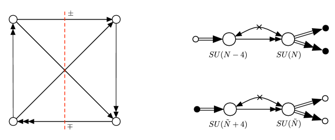
Figure 5: The left side shows the quiver gauge theory for $dP_{1}$, with the involution of interest indicated by the dashed line. The resulting quiverfold (see appendix A) theories for the two sign choices are shown on the right.

Moreover, only two choices for these signs lead to theories which can be anomaly free without the addition of noncompact “flavor” D7 branes. As we show in transitions3 using brane tiling methods, these involutions also satisfy rule II and lead to superpotentials which inherit the $SU(2)\times U(1)_{X}\times U(1)_{R}$ geometric flavor symmetries of the parent theory, as expected for a compact O7 plane.

The two possible sign choices lead to the orientifold gauge theory

$$\begin{array}[]{c|cc|ccccc}&SU(N-4)&SU(N)&SU(2)&U(1)_{X}&U(1)_{B}&U(1)_{R}\\ \hline\cr A^{i}&\leavevmode\hbox{\vtop{\offinterlineskip\openup-0.4pt\halign{&\startbox@YT{\defarg@YT}{}#\endbox@YT\cr\framebox{\vbox to5.0pt{\vss\hbox to5.0pt{\hss$$\hss}\vss}}\cr}}\kern 5.0pt}&\overline{}\leavevmode\hbox{\vtop{\offinterlineskip\openup-0.4pt\halign{&\startbox@YT{\defarg@YT}{}#\endbox@YT\cr\framebox{\vbox to5.0pt{\vss\hbox to5.0pt{\hss$$\hss}\vss}}\cr}}\kern 5.0pt}&\leavevmode\hbox{\vtop{\offinterlineskip\openup-0.4pt\halign{&\startbox@YT{\defarg@YT}{}#\endbox@YT\cr\framebox{\vbox to5.0pt{\vss\hbox to5.0pt{\hss$$\hss}\vss}}\cr}}\kern 5.0pt}&\frac{N-2}{N-4}&-\frac{2(N-1)}{N(N-4)}&-\frac{8}{N(N-4)}\\ Y&\overline{}\leavevmode\hbox{\vtop{\offinterlineskip\openup-0.4pt\halign{&\startbox@YT{\defarg@YT}{}#\endbox@YT\cr\framebox{\vbox to5.0pt{\vss\hbox to5.0pt{\hss$$\hss}\vss}}\cr}}\kern 5.0pt}&\overline{}\leavevmode\hbox{\vtop{\offinterlineskip\openup-0.4pt\halign{&\startbox@YT{\defarg@YT}{}#\endbox@YT\cr\framebox{\vbox to5.0pt{\vss\hbox to5.0pt{\hss$$\hss}\vss}}\cr}}\kern 5.0pt}&{\bf 1}&-\frac{N-2}{N-4}&\frac{(N+2)}{N(N-4)}&\frac{N^{2}-8}{N(N-4)}\\ Z&\overline{}\leavevmode\hbox{\vtop{\offinterlineskip\openup-0.4pt\halign{&\startbox@YT{\defarg@YT}{}#\endbox@YT\cr\framebox{\vbox to5.0pt{\vss\hbox to5.0pt{\hss$$\hss}\vss}}&\framebox{\vbox to5.0pt{\vss\hbox to5.0pt{\hss$$\hss}\vss}}\cr}}\kern 10.0pt}&{\bf 1}&{\bf 1}&-\frac{N}{N-4}&\frac{3}{N-4}&\frac{N}{N-4}\\ B^{i}&{\bf 1}&\leavevmode\hbox{\vtop{\offinterlineskip\openup-0.4pt\halign{&\startbox@YT{\defarg@YT}{}#\endbox@YT\cr\framebox{\vbox to5.0pt{\vss\hbox to5.0pt{\hss$$\hss}\vss}}\cr\framebox{\vbox to5.0pt{\vss\hbox to5.0pt{\hss$$\hss}\vss}}\cr}}\kern 5.0pt}&\leavevmode\hbox{\vtop{\offinterlineskip\openup-0.4pt\halign{&\startbox@YT{\defarg@YT}{}#\endbox@YT\cr\framebox{\vbox to5.0pt{\vss\hbox to5.0pt{\hss$$\hss}\vss}}\cr}}\kern 5.0pt}&0&\frac{1}{N}&\frac{N-4}{N}\\ X&{\bf 1}&\leavevmode\hbox{\vtop{\offinterlineskip\openup-0.4pt\halign{&\startbox@YT{\defarg@YT}{}#\endbox@YT\cr\framebox{\vbox to5.0pt{\vss\hbox to5.0pt{\hss$$\hss}\vss}}\cr\framebox{\vbox to5.0pt{\vss\hbox to5.0pt{\hss$$\hss}\vss}}\cr}}\kern 5.0pt}&{\bf 1}&-1&\frac{1}{N}&\frac{N-4}{N}\end{array}$$ (284)

with superpotential

$$W=\epsilon_{ij}\mathrm{Tr\,}[B^{i}A^{j}Y+XA^{i}ZA^{j}]\,,$$ (285)

as well as the theory

$$\begin{array}[]{c|cc|ccccc}&SU(\tilde{N}+4)&SU(\tilde{N})&SU(2)&U(1)_{X}&U(1)_{B}&U(1)_{R}\\ \hline\cr\tilde{A}^{i}&\leavevmode\hbox{\vtop{\offinterlineskip\openup-0.4pt\halign{&\startbox@YT{\defarg@YT}{}#\endbox@YT\cr\framebox{\vbox to5.0pt{\vss\hbox to5.0pt{\hss$$\hss}\vss}}\cr}}\kern 5.0pt}&\overline{}\leavevmode\hbox{\vtop{\offinterlineskip\openup-0.4pt\halign{&\startbox@YT{\defarg@YT}{}#\endbox@YT\cr\framebox{\vbox to5.0pt{\vss\hbox to5.0pt{\hss$$\hss}\vss}}\cr}}\kern 5.0pt}&\leavevmode\hbox{\vtop{\offinterlineskip\openup-0.4pt\halign{&\startbox@YT{\defarg@YT}{}#\endbox@YT\cr\framebox{\vbox to5.0pt{\vss\hbox to5.0pt{\hss$$\hss}\vss}}\cr}}\kern 5.0pt}&\frac{\tilde{N}+2}{\tilde{N}+4}&-\frac{2(\tilde{N}+1)}{\tilde{N}(\tilde{N}+4)}&-\frac{8}{\tilde{N}(\tilde{N}+4)}\\ \tilde{Y}&\overline{}\leavevmode\hbox{\vtop{\offinterlineskip\openup-0.4pt\halign{&\startbox@YT{\defarg@YT}{}#\endbox@YT\cr\framebox{\vbox to5.0pt{\vss\hbox to5.0pt{\hss$$\hss}\vss}}\cr}}\kern 5.0pt}&\overline{}\leavevmode\hbox{\vtop{\offinterlineskip\openup-0.4pt\halign{&\startbox@YT{\defarg@YT}{}#\endbox@YT\cr\framebox{\vbox to5.0pt{\vss\hbox to5.0pt{\hss$$\hss}\vss}}\cr}}\kern 5.0pt}&{\bf 1}&-\frac{\tilde{N}+2}{\tilde{N}+4}&\frac{(\tilde{N}-2)}{\tilde{N}(\tilde{N}+4)}&\frac{\tilde{N}^{2}-8}{\tilde{N}(\tilde{N}+4)}\\ \tilde{Z}&\overline{}\leavevmode\hbox{\vtop{\offinterlineskip\openup-0.4pt\halign{&\startbox@YT{\defarg@YT}{}#\endbox@YT\cr\framebox{\vbox to5.0pt{\vss\hbox to5.0pt{\hss$$\hss}\vss}}\cr\framebox{\vbox to5.0pt{\vss\hbox to5.0pt{\hss$$\hss}\vss}}\cr}}\kern 5.0pt}&{\bf 1}&{\bf 1}&-\frac{\tilde{N}}{\tilde{N}+4}&\frac{3}{\tilde{N}+4}&\frac{\tilde{N}}{\tilde{N}+4}\\ \tilde{B}^{i}&{\bf 1}&\leavevmode\hbox{\vtop{\offinterlineskip\openup-0.4pt\halign{&\startbox@YT{\defarg@YT}{}#\endbox@YT\cr\framebox{\vbox to5.0pt{\vss\hbox to5.0pt{\hss$$\hss}\vss}}&\framebox{\vbox to5.0pt{\vss\hbox to5.0pt{\hss$$\hss}\vss}}\cr}}\kern 10.0pt}&\leavevmode\hbox{\vtop{\offinterlineskip\openup-0.4pt\halign{&\startbox@YT{\defarg@YT}{}#\endbox@YT\cr\framebox{\vbox to5.0pt{\vss\hbox to5.0pt{\hss$$\hss}\vss}}\cr}}\kern 5.0pt}&0&\frac{1}{\tilde{N}}&\frac{\tilde{N}+4}{\tilde{N}}\\ \tilde{X}&{\bf 1}&\leavevmode\hbox{\vtop{\offinterlineskip\openup-0.4pt\halign{&\startbox@YT{\defarg@YT}{}#\endbox@YT\cr\framebox{\vbox to5.0pt{\vss\hbox to5.0pt{\hss$$\hss}\vss}}&\framebox{\vbox to5.0pt{\vss\hbox to5.0pt{\hss$$\hss}\vss}}\cr}}\kern 10.0pt}&{\bf 1}&-1&\frac{1}{\tilde{N}}&\frac{\tilde{N}+4}{\tilde{N}}\end{array}$$ (302)

with superpotential

$$W=\epsilon_{ij}\mathrm{Tr\,}[\tilde{B}^{i}\tilde{A}^{j}\tilde{Y}+\tilde{X}\tilde{A}^{i}\tilde{Z}\tilde{A}^{j}]\,,$$ (303)

where in either case the gauge indices are cyclically contracted. Henceforward, for want of a better label we refer to these theories as “Theory A” and “Theory B”, respectively. For ease of presentation we have chosen a basis for the R-symmetry which does not satisfy a-maximization, as the superconformal R-charges are irrational.

The global anomalies for both theories are shown in table 4.

$$\begin{array}[]{|c|c|c|}\lx@intercol\hfil\text{Theory A}\qquad\qquad\text{Theory B}\lx@intercol\\ \hline\cr SU(2)^{3}&(-1)^{\frac{3}{2}N(N-3)}&(-1)^{\frac{3}{2}\tilde{N}(\tilde{N}+3)}\\ \hline\cr SU(2)^{2}\,U(1)_{X}&N(N-2)&\tilde{N}(\tilde{N}+2)\\ \hline\cr SU(2)^{2}\,U(1)_{B}&-\frac{3}{2}(N-1)&-\frac{3}{2}(\tilde{N}+1)\\ \hline\cr U(1)_{X}^{2}\,U(1)_{B}&-(N-1)&-(\tilde{N}+1)\\ \hline\cr U(1)_{X}\,U(1)_{B}^{2}&2&2\\ \hline\cr SU(2)^{2}\,U(1)_{R}&-N(N-2)-6&-\tilde{N}(\tilde{N}+2)-6\\ \hline\cr U(1)_{X}^{2}\,U(1)_{R}&-2N(N-2)-4&-2\tilde{N}(\tilde{N}+2)-4\\ \hline\cr U(1)_{B}^{2}\,U(1)_{R}&-8&-8\\ \hline\cr U(1)_{X}\,U(1)_{B}\,U(1)_{R}&4(N-1)&4(\tilde{N}+1)\\ \hline\cr U(1)_{X}\,U(1)_{R}^{2}&2N(N-2)&2\tilde{N}(\tilde{N}+2)\\ \hline\cr U(1)_{B}\,U(1)_{R}^{2}&-4(N-1)&-4(\tilde{N}+1)\\ \hline\cr U(1)_{R}^{3}&-34&-34\\ \hline\cr U(1)_{R}&-10&-10\\ \hline\cr\end{array}$$

Table 4: The nonvanishing anomalies for theory A and theory B, where we use a multiplicative notation for the $SU(2)^{3}$ Witten anomaly analogous to that used for discrete symmetries in §3.1. The $U(1)_{B}^{3}$, $U(1)_{X}^{3}$, $U(1)_{B}$, and $U(1)_{X}$ anomalies vanish in both theories.

We see that the anomalies match between the two theories for $\tilde{N}=N-2$ provided that $N$ is odd. For even $N$ the $SU(2)^{3}$ Witten anomalies do not match, and the theories are not dual.

For completeness, we also present the $a$-maximizing superconformal R-charge, which is a linear combination:

$$U(1)_{R}^{\rm(sc)}=U(1)_{R}+a_{X}U(1)_{X}+a_{B}U(1)_{B}\,.$$ (304)

A-maximization in theory A gives

$$a_{B}=\frac{a_{X}^{2}-8a_{X}+4}{4(a_{X}-4)}(N-1)\,,$$ (305)

where $a_{X}$ is a solution to the quartic equation

$$0=(N-1)^{2}(a_{X}^{2}-4)[3a_{X}^{2}-16a_{X}+4]+16(2a_{X}+1)(a_{X}-4)^{2}\,,$$ (306)

in the range $a_{X}\in\left(-\frac{1}{2},\frac{2}{3}(4-\sqrt{13})\right)$, whereas exactly one solution lies in this range for any $N>1$. For example, we obtain approximately

$$\begin{array}[]{c|cccccccccccc}\!N\!&2&3&4&5&6&7&8&9&10&11&12\\ \hline\cr\!a_{X}\!&\!-0.431\!&\!-0.270\!&\!-0.113\!&0&\!0.074\!&\!0.122\!&\!0.155\!&\!0.178\!&\!0.194\!&\!0.207\!&\!0.216\!\end{array}$$ (309)

The result for $N=5$ is exact, giving $a_{X}=0$ and $a_{B}=-1$. For large $N$, $a_{X}$ asymptotically approaches $\frac{2}{3}(4-\sqrt{13})\approx 0.263$. The same considerations apply in theory B upon replacing $N-1\to\tilde{N}+1$.

In the following sections, we explore the prospective duality for odd $N$. We will also have more to say about the case of even $N$ in the next section.

6.1.1 Moduli space and Higgsing

We begin by considering the mapping between the moduli spaces of the two theories, which is equivalently expressed as a map between the holomorphic gauge invariants subject to the F-term conditions.

To obtain this map, we consider certain “minimal” operators, i.e. operators whose $U(1)$ charges cannot be obtained as the sum of the $U(1)$ charges of two or more nonvanishing operators. Operators of this type can only mix with other minimal operators under the duality, whereas generically no two minimal operators share the same $U(1)$ charges, leading to a unique matching between the minimal operators of the dual theories.

To find minimal operators, we begin by classifying irreducible “gauge-invariant” monomials in the fundamental fields, i.e. formal products of the fields (disregarding gauge-indices) which are neutral under the $\mathbb{Z}_{N-4}\times\mathbb{Z}_{N}$ or $\mathbb{Z}_{\tilde{N}+4}\times\mathbb{Z}_{\tilde{N}}$ gauge-group center, and which cannot be factored into two or more gauge-invariant pieces. The resulting finite list generates all gauge-invariant monomials, a subset of which will correspond to actual gauge-invariant operators. Using this classification, it is possible to show that certain candidate operators are minimal.

Using these methods, we obtain the following minimal operators in theory A for odd $N$:

$$\begin{array}[]{c|ccc}&U(1)_{B}&U(1)_{X}^{\prime}&U(1)_{R}^{\prime}\\ \hline\cr A^{2}(Y|AZ)^{2}(B|X)^{2}&0&[-2,2]&4\\ B^{2}X(B|X)^{N-3}&1&[-\frac{N-3}{2},\frac{N-3}{2}]&N-5\\ Z^{N-4-2k}(Y^{2}X)^{2k}&3&\frac{N-3}{2}-4k&N-3+4k\\ A^{N-4}B(B|X)^{N-3}&-1&[-\frac{N-3}{2},\frac{N-3}{2}]&N-5\\ A^{N}(Y|AZ)^{4}(B|X)^{2}&-2&[-3,3]&8\\ A^{p(N-4)}(B|X)^{N-2p}&1-2p&[-\frac{N+1-2p}{2},\frac{N-1-2p}{2}]&N-5\end{array}$$ (317)

where $2\leq p\leq\frac{N-1}{2}$, $(x|y)^{n}$ denotes a monomial of degree $n$ in $x$ and $y$, and we employ a slightly different basis for the $U(1)$ charges:

$$U(1)_{X}^{\prime}=U(1)_{X}+\frac{N-1}{2}U(1)_{B}\,,\quad U(1)_{R}^{\prime}=U(1)_{R}-U(1)_{B}\,.$$ (318)

A similar analysis in theory B for odd $\tilde{N}$ gives

$$\begin{array}[]{c|ccc}&U(1)_{B}&U(1)_{X}^{\prime}&U(1)_{R}^{\prime}\\ \hline\cr\tilde{A}^{2}(\tilde{Y}|\tilde{A}\tilde{Z})^{2}(\tilde{B}|\tilde{X})^{2}&0&[-2,2]&4\\ \tilde{Y}\tilde{Z}^{2}(\tilde{Y}|\tilde{A}\tilde{Z})^{\tilde{N}-1}&1&[-\frac{\tilde{N}-1}{2},\frac{\tilde{N}-1}{2}]&\tilde{N}-3\\ \tilde{Z}^{\tilde{N}+3-2k}(\tilde{Y}^{2}\tilde{X})^{2k+1}&3&\frac{\tilde{N}-1}{2}-4k&\tilde{N}-1+4k\\ \tilde{A}^{\tilde{N}+1}\tilde{Z}(\tilde{Y}|\tilde{A}\tilde{Z})^{\tilde{N}-1}&-1&[-\frac{\tilde{N}-1}{2},\frac{\tilde{N}-1}{2}]&\tilde{N}-3\\ \tilde{A}^{\tilde{N}+6}(\tilde{Y}|\tilde{A}\tilde{Z})^{2}(\tilde{B}|\tilde{X})^{4}&-2&[-3,3]&8\\ \tilde{A}^{p(\tilde{N}+2)-2}(\tilde{Y}|\tilde{A}\tilde{Z})^{\tilde{N}+2-2p}&1-2p&[-\frac{\tilde{N}+3-2p}{2},\frac{\tilde{N}+1-2p}{2}]&\tilde{N}-3\end{array}$$ (326)

Thus, the spectrum of minimal operators appears to match between the two theories for $\tilde{N}=N-2$, a highly nontrivial check of the proposed duality.

Several comments are in order. Firstly, while this may not comprise a complete list of minimal operators, one can show that all of the listed operators are minimal, and that no other minimal operators share the same $U(1)$ charges, so the matching is reliable. Secondly, to obtain this matching, it is necessary to carefully account for the structure of the gauge-index contraction as well as the F-term conditions. For example, consider the operator $Z^{N-4-p}(Y^{2}X)^{p}$. Each $X$ factor must appear in the combination $X^{mn}Y^{a}_{m}Y^{b}_{n}$, which is therefore antisymmetric in the $SU(N-4)$ indices. Since $Z^{ab}$ is symmetric, a gauge invariant index contraction exists if and only if an even number of $XY^{2}$ factors appear, i.e. if and only if $p$ is even. By contrast, in the operator $\tilde{Z}^{\tilde{N}+4-p}(\tilde{Y}^{2}\tilde{X})^{p}$ the symmetry properties are reversed, and an even number $\tilde{Z}$ factors must appear, i.e. $p$ must be odd (since $\tilde{N}$ is odd).

These particular operators are also interesting in that they correspond to Higgsing to the $dP_{0}$ theories studied in §3. In particular, the operator $Z^{N-4-2k}(Y^{2}X)^{2k}$ corresponds to Higgsing the A theory $SU(N-4)\times SU(N)$ to $SO(N-4-2k)\times SU(N-2k)$, whereas the operator $\tilde{Z}^{\tilde{N}+3-2k}(\tilde{Y}^{2}\tilde{X})^{2k+1}$ corresponds to Higgsing the B theory $SU(\tilde{N}+4)\times SU(\tilde{N})$ to $U\!Sp(\tilde{N}+3-2k)\times SU(\tilde{N}-2k-1)$. Consistent with the proposed operator mapping, we observe that the resulting theories are related by the duality proposed in §3. This is another nontrivial consistency check.

At this point, it is also instructive to consider the behavior of the even-$N$ theories under Higgsing. Turning on a vev for $Z^{N-4-2k}(Y^{2}X)^{2k}$ once again corresponds to Higgsing theory A to $SO(N-4-2k)\times SU(N-2k)$, where now the resulting theory is conjectured to be self-dual under S-duality, suggesting that the A theory for even $N$ is also self-dual. However, things are quite different in the even-$\tilde{N}$ B theory. Here, the simplest Higgsing, corresponding to the operator $\tilde{Z}^{(\tilde{N}+4)/2}$, breaks $SU(\tilde{N}+4)\times SU(\tilde{N})$ to $U\!Sp(\tilde{N}+4)\times SU(\tilde{N})$, where now the resulting theory is not a singlet under S-duality, inconsistent with self-duality for the parent theory, while on the other hand there is no candidate dual for the parent theory.

We hypothesize that the even-$\tilde{N}$ B theory is inconsistent in string theory, potentially due to an uncanceled K-theory (discrete) tadpole. We hope to verify this through explicit computation of the K-theory tadpoles in future work.

Having discussed some generic features of the proposed odd-$N$ duality, we next discuss a particularly tractable example with a deformed quantum moduli space.

6.1.2 Case study: the $SU(5)\longleftrightarrow SU(7)\times SU(3)$ duality

The lowest rank example of the proposed duality between the A and B theories is for $N=5$. This example turns out to be particularly tractable, and we now show that the dual theories have biholomorphic quantum-deformed moduli spaces. The $SU(7)\times SU(3)$ theory turns out to be somewhat more intuitive, so we begin by discussing this theory, after which we briefly explain how to show that the $SU(5)$ theory has the same moduli space.

Theory B

We consider the B-theory $SU(7)\times SU(3)$:

$$\begin{array}[]{c|cc|cccc}&SU(7)&SU(3)&SU(2)&U(1)_{B}&U(1)_{X}^{\prime}&U(1)_{R}^{\prime}\\ \hline\cr\tilde{A}^{i}&\overline{}\leavevmode\hbox{\vtop{\offinterlineskip\openup-0.4pt\halign{&\startbox@YT{\defarg@YT}{}#\endbox@YT\cr\framebox{\vbox to5.0pt{\vss\hbox to5.0pt{\hss$$\hss}\vss}}\cr}}\kern 5.0pt}&\leavevmode\hbox{\vtop{\offinterlineskip\openup-0.4pt\halign{&\startbox@YT{\defarg@YT}{}#\endbox@YT\cr\framebox{\vbox to5.0pt{\vss\hbox to5.0pt{\hss$$\hss}\vss}}\cr}}\kern 5.0pt}&\leavevmode\hbox{\vtop{\offinterlineskip\openup-0.4pt\halign{&\startbox@YT{\defarg@YT}{}#\endbox@YT\cr\framebox{\vbox to5.0pt{\vss\hbox to5.0pt{\hss$$\hss}\vss}}\cr}}\kern 5.0pt}&-\frac{8}{21}&-\frac{1}{21}&0\\ \tilde{Y}&\leavevmode\hbox{\vtop{\offinterlineskip\openup-0.4pt\halign{&\startbox@YT{\defarg@YT}{}#\endbox@YT\cr\framebox{\vbox to5.0pt{\vss\hbox to5.0pt{\hss$$\hss}\vss}}\cr}}\kern 5.0pt}&\leavevmode\hbox{\vtop{\offinterlineskip\openup-0.4pt\halign{&\startbox@YT{\defarg@YT}{}#\endbox@YT\cr\framebox{\vbox to5.0pt{\vss\hbox to5.0pt{\hss$$\hss}\vss}}\cr}}\kern 5.0pt}&\mathbf{1}&\frac{1}{21}&-\frac{13}{21}&0\\ \tilde{Z}&\leavevmode\hbox{\vtop{\offinterlineskip\openup-0.4pt\halign{&\startbox@YT{\defarg@YT}{}#\endbox@YT\cr\framebox{\vbox to5.0pt{\vss\hbox to5.0pt{\hss$$\hss}\vss}}\cr\framebox{\vbox to5.0pt{\vss\hbox to5.0pt{\hss$$\hss}\vss}}\cr}}\kern 5.0pt}&\mathbf{1}&\mathbf{1}&\frac{3}{7}&\frac{3}{7}&0\\ \tilde{B}^{i}&\mathbf{1}&\overline{}\leavevmode\hbox{\vtop{\offinterlineskip\openup-0.4pt\halign{&\startbox@YT{\defarg@YT}{}#\endbox@YT\cr\framebox{\vbox to5.0pt{\vss\hbox to5.0pt{\hss$$\hss}\vss}}&\framebox{\vbox to5.0pt{\vss\hbox to5.0pt{\hss$$\hss}\vss}}\cr}}\kern 10.0pt}&\leavevmode\hbox{\vtop{\offinterlineskip\openup-0.4pt\halign{&\startbox@YT{\defarg@YT}{}#\endbox@YT\cr\framebox{\vbox to5.0pt{\vss\hbox to5.0pt{\hss$$\hss}\vss}}\cr}}\kern 5.0pt}&\frac{1}{3}&\frac{2}{3}&2\\ \tilde{X}&\mathbf{1}&\overline{}\leavevmode\hbox{\vtop{\offinterlineskip\openup-0.4pt\halign{&\startbox@YT{\defarg@YT}{}#\endbox@YT\cr\framebox{\vbox to5.0pt{\vss\hbox to5.0pt{\hss$$\hss}\vss}}&\framebox{\vbox to5.0pt{\vss\hbox to5.0pt{\hss$$\hss}\vss}}\cr}}\kern 10.0pt}&\mathbf{1}&\frac{1}{3}&-\frac{1}{3}&2\end{array}$$ (343)

with the superpotential:

$$W=\tilde{\lambda}\,\epsilon_{ij}\mathrm{Tr\,}[\tilde{B}^{i}\tilde{A}^{j}\tilde{Y}]+\frac{1}{2\tilde{\mu}}\epsilon_{ij}\mathrm{Tr\,}[\tilde{X}\tilde{A}^{i}\tilde{Z}\tilde{A}^{j}]\,.$$ (344)

All possible $SU(7)$ gauge invariants are products of the following:

$$\mathcal{Y}^{Im} \equiv \tilde{A}^{I}_{a}\tilde{Y}^{a;m}\,,\quad\mathcal{Q}^{m}\equiv\frac{1}{48}\epsilon_{abcdefg}\tilde{Y}^{a;m}\tilde{Z}^{bc}\tilde{Z}^{de}\tilde{Z}^{fg}\,,$$ (345)

$$\mathcal{Z}^{IJ} \equiv \tilde{A}^{I}_{a}\tilde{A}^{J}_{b}\tilde{Z}^{ab}\,,\quad\,\Phi\equiv\frac{1}{48}\epsilon_{mnp}\epsilon_{abcdefg}\tilde{Y}^{a;m}\tilde{Y}^{b;n}\tilde{Y}^{c;p}\tilde{Z}^{de}\tilde{Z}^{fg}\,,$$

where $a,b,\ldots$ index $SU(7)$, $m,n,\ldots$ index $SU(3)$, and $I,J,\ldots$ index a fictitious $SU(6)\supset SU(3)\times SU(2)$. There is a classical constraint:

$$\frac{1}{2}\epsilon_{mnp}(\mathrm{Pcf}\mathcal{Z})_{IJ}\mathcal{Y}^{Im}\mathcal{Y}^{Jn}\mathcal{Q}^{p}=(\mathrm{Pf}\mathcal{Z})\Phi\,,$$ (346)

where we define

$$\mathrm{Pf}M \equiv \frac{1}{2^{n}n!}\epsilon_{i_{1}j_{1}\ldots i_{n}j_{n}}M^{i_{1}j_{1}}\ldots M^{i_{n}j_{n}}\,,$$ (347)

$$(\mathrm{Pcf}M)_{ij} \equiv \frac{1}{2^{n-1}(n-1)!}\epsilon_{iji_{2}j_{2}\ldots i_{n}j_{n}}M^{i_{2}j_{2}}\ldots M^{i_{n}j_{n}}\,,$$

for a $2n\times 2n$ antisymmetric matrix $M^{ij}$ and “Pcf” stands for “Pfaffian cofactor”, since for $M$ invertible it takes the form $\mathrm{Pcf}M=(\mathrm{Pf}M)[M^{-1}]^{T}$, much like $\mathrm{cof}M=(\det M)[M^{-1}]^{T}$ for an arbitrary invertible matrix $M$.

The classical constraint is quantum modified to Poppitz:1995fh

$$\frac{1}{2}\epsilon_{mnp}(\mathrm{Pcf}\mathcal{Z})_{IJ}\mathcal{Y}^{Im}\mathcal{Y}^{Jn}\mathcal{Q}^{p}-(\mathrm{Pf}\mathcal{Z})\Phi=\Lambda_{SU(7)}^{14}\,.$$ (348)

This equation describes the quantum moduli space of the $SU(7)$ gauge theory when we take the $SU(3)$ gauge coupling and superpotential couplings to zero.

We now account for the finiteness of these couplings. In particular, the superpotential couplings give a mass to certain components of $\mathcal{Y}$ and $\mathcal{Z}$, so that on the moduli space we must have

$$\mathcal{Y}^{m_{i}n}=\epsilon^{mnp}\mathcal{Y}^{i}_{p}\,,\quad\mathcal{Z}^{m_{i}n_{j}}=\epsilon^{mnp}\mathcal{Z}^{ij}_{p}\,,$$ (349)

where $m_{i}=m+3(i-1)$ indexes the fictitious $SU(6)$. Since the LHS of (348) contains only $SU(3)$ baryons built from $SU(3)$ fundamentals, $SU(3)$ is completely broken everywhere in the moduli space, leading to a confined description where the effect of gauging $SU(3)$ is to remove 8 Higgsed degrees of freedom and their superpartners.

Thus, the moduli space is parameterized by the operators:

$$\begin{array}[]{c|c|cccc}&SU(3)&SU(2)&U(1)_{B}&U(1)_{X}^{\prime}&U(1)_{R}^{\prime}\\ \hline\cr\mathcal{Y}^{{}_{i}}_{m}=(\tilde{Y}\tilde{A}^{i})&\overline{}\leavevmode\hbox{\vtop{\offinterlineskip\openup-0.4pt\halign{&\startbox@YT{\defarg@YT}{}#\endbox@YT\cr\framebox{\vbox to5.0pt{\vss\hbox to5.0pt{\hss$$\hss}\vss}}\cr}}\kern 5.0pt}&\mathbf{2}&-\frac{1}{3}&-\frac{2}{3}&0\\ \mathcal{Z}^{ij}_{m}=(\tilde{Z}\tilde{A}^{i}\tilde{A}^{j})&\overline{}\leavevmode\hbox{\vtop{\offinterlineskip\openup-0.4pt\halign{&\startbox@YT{\defarg@YT}{}#\endbox@YT\cr\framebox{\vbox to5.0pt{\vss\hbox to5.0pt{\hss$$\hss}\vss}}\cr}}\kern 5.0pt}&\mathbf{3}&-\frac{1}{3}&\frac{1}{3}&0\\ \mathcal{Q}^{m}=(\tilde{Z}^{3}\tilde{Y})&\leavevmode\hbox{\vtop{\offinterlineskip\openup-0.4pt\halign{&\startbox@YT{\defarg@YT}{}#\endbox@YT\cr\framebox{\vbox to5.0pt{\vss\hbox to5.0pt{\hss$$\hss}\vss}}\cr}}\kern 5.0pt}&\mathbf{1}&\frac{4}{3}&\frac{2}{3}&0\\ \Phi=(\tilde{Z}^{2}\tilde{Y}^{3})&\mathbf{1}&\mathbf{1}&1&-1&0\end{array}$$ (358)

subject to the gauging of $SU(3)$ and the quantum-modified constraint. Therefore, the dimension of the moduli space is:

$$\dim\mathcal{M}=19-8-1=10\,.$$ (359)

Since all operators are neutral under $U(1)_{R}^{\prime}$, there is an unbroken $U(1)_{R}^{\prime}$ everywhere in the moduli space.

A complete list of $SU(3)$ gauge invariants formed from these four fields is:

$$\begin{array}[]{c|cccc}&SU(2)&U(1)_{B}&U(1)_{X}^{\prime}&U(1)_{R}^{\prime}\\ \hline\cr\mathcal{Y}^{2}\mathcal{Z}&\mathbf{3}&-1&-1&0\\ \mathcal{Y}\mathcal{Z}^{2}&\mathbf{4}\oplus\mathbf{2}&-1&0&0\\ \mathcal{Z}^{3}&\mathbf{1}&-1&1&0\\ \mathcal{Z}\mathcal{Q}&\mathbf{3}&1&1&0\\ \mathcal{Y}\mathcal{Q}&\mathbf{2}&1&0&0\\ \Phi&\mathbf{1}&1&-1&0\end{array}$$ (367)

Since there are a total of 16 invariants, still subject to one modified constraint, we conclude that there are five further “classical” constraints relating these $SU(3)$ composites. To make these constraints explicit, we define:

$$\bar{\mathcal{Q}}^{A}_{m}\equiv\{\mathcal{Y}^{i}_{m},\mathcal{Z}^{\alpha}_{m}\}\,,$$ (368)

where $A$ indexes a fictitious $SU(5)\supset SU(2)\times SO(3)$, and $\mathcal{Z}^{\alpha}_{m}\equiv\frac{1}{2}\sigma^{\alpha}_{ij}\mathcal{Z}^{ij}_{m}$ with the $SU(2)\cong SO(3)$ conventions:

$$\sigma^{\alpha\;j}_{i}=\left\{\left(\begin{array}[]{cc}0&1\\ 1&0\end{array}\right),\left(\begin{array}[]{cc}0&-i\\ i&0\end{array}\right),\left(\begin{array}[]{cc}1&0\\ 0&-1\end{array}\right)\right\},\;\;\sigma^{ij}_{\alpha}=\epsilon^{ik}\sigma^{\alpha\;j}_{k}\,,\;\;\sigma^{\alpha}_{ij}=\sigma^{\alpha\;k}_{i}\epsilon_{kj}\,,\;\;\epsilon^{12}=\epsilon_{12}=+1\,.$$ (375)

The classical constraints then take the form:

$${}[\bar{\mathcal{Q}}^{3}]_{AB}[\mathcal{Q}\bar{\mathcal{Q}}]^{B}=0\,,\quad\epsilon^{ABCDE}[\bar{\mathcal{Q}}^{3}]_{AB}[\bar{\mathcal{Q}}^{3}]_{CD}=0\,.$$ (376)

Although both equations appear to have five components, examining small fluctuations about a background with $\bar{\mathcal{Q}}\neq 0$ satisfying these constraints gives only three independent constraints from the second equation, and a further two from the first, for a total of five constraints, as expected.

We define:

$$\Psi \equiv \det\mathcal{Z}^{\alpha}_{m}\,,\quad\Psi^{i}_{\alpha}\equiv\mathcal{Y}^{i}_{m}[\mathrm{cof}\mathcal{Z}]^{m}_{\alpha}\,,\quad\Psi^{\alpha}\equiv\frac{1}{2}\epsilon_{ij}\epsilon^{mnp}\mathcal{Y}^{i}_{m}\mathcal{Y}^{j}_{n}\mathcal{Z}^{\alpha}_{p}\,,$$ (377)

$$\Phi^{i} \equiv \mathcal{Q}^{m}\mathcal{Y}_{m}^{i}\,,\quad\,\Phi^{\alpha}\equiv\mathcal{Q}^{m}\mathcal{Z}_{m}^{\alpha}\,.$$ (378)

In terms of these gauge invariants, the classical constraints becomes:

$$\Psi\Phi^{j}-\Psi^{j}_{\alpha}\Phi^{\alpha}=0\,,\;\;\epsilon_{ij}\Psi^{i}_{\alpha}\Phi^{j}+\epsilon_{\alpha\beta\gamma}\Psi^{\beta}\Phi^{\gamma}=0\,,$$ (379)

and

$$\Psi^{i}_{\alpha}\Psi^{\alpha}=0\,,\;\;\Psi\Psi^{\alpha}-\frac{1}{2}\epsilon^{\alpha\beta\gamma}\epsilon_{ij}\Psi^{i}_{\beta}\Psi^{j}_{\gamma}=0\,.$$ (380)

After a somewhat longer computation, we find that the quantum modified constraint takes the form:

$$i\Phi^{i}\Psi^{j}_{\alpha}\sigma^{\alpha}_{ij}-\Phi_{\alpha}\Psi^{\alpha}-2i\Phi\Psi=\Lambda^{14}_{SU(7)}\,.$$ (381)

Together, (379, 380, 381) completely describe the deformed moduli space of the quantum theory.

The maximal unbroken flavor symmetry is $SU(2)\times U(1)_{B+X}^{\prime}\times U(1)_{R}^{\prime}$, which is attained when we take $\Phi$ and $\Psi$ to be nonvanishing with all other fields vanishing. We can then solve the constraints to eliminate $\Phi^{i}$, $\Psi^{\alpha}$, and $\Phi$:

$$\Phi^{i}=\frac{1}{\Psi}\Psi^{i}_{\alpha}\Phi^{\alpha}\,,\quad\Psi^{\alpha}=\frac{1}{2\Psi}\epsilon^{\alpha\beta\gamma}\epsilon_{ij}\Psi^{i}_{\beta}\Psi^{j}_{\gamma}\,,\quad\Phi=\frac{i}{2\Psi}\Lambda^{14}_{SU(7)}\,,$$ (382)

whereupon the remaining constraints are trivially satisfied. The light modes along this line are therefore:

$$\begin{array}[]{c|ccc}&SU(2)&U(1)_{B+X}^{\prime}&U(1)_{R}^{\prime}\\ \hline\cr\Psi^{i}_{\alpha}&\mathbf{4}\oplus\mathbf{2}&-1&0\\ \Psi&\mathbf{1}&0&0\\ \Phi^{\alpha}&\mathbf{3}&2&0\end{array}$$ (387)

One can check that the global $SU(2)\times U(1)_{B+X}^{\prime}\times U(1)_{R}^{\prime}$ anomalies match those of the original description, as expected.

Theory A

We now consider the dual theory:

$$\begin{array}[]{c|c|cccc}&SU(5)&SU(2)&U(1)_{B}&U(1)_{X}^{\prime}&U(1)_{R}^{\prime}\\ \hline\cr A^{i}&\overline{}\leavevmode\hbox{\vtop{\offinterlineskip\openup-0.4pt\halign{&\startbox@YT{\defarg@YT}{}#\endbox@YT\cr\framebox{\vbox to5.0pt{\vss\hbox to5.0pt{\hss$$\hss}\vss}}\cr}}\kern 5.0pt}&\leavevmode\hbox{\vtop{\offinterlineskip\openup-0.4pt\halign{&\startbox@YT{\defarg@YT}{}#\endbox@YT\cr\framebox{\vbox to5.0pt{\vss\hbox to5.0pt{\hss$$\hss}\vss}}\cr}}\kern 5.0pt}&-\frac{8}{5}&-\frac{1}{5}&0\\ Y&\overline{}\leavevmode\hbox{\vtop{\offinterlineskip\openup-0.4pt\halign{&\startbox@YT{\defarg@YT}{}#\endbox@YT\cr\framebox{\vbox to5.0pt{\vss\hbox to5.0pt{\hss$$\hss}\vss}}\cr}}\kern 5.0pt}&\mathbf{1}&\frac{7}{5}&-\frac{1}{5}&2\\ Z&\mathbf{1}&\mathbf{1}&3&1&2\\ B^{i}&\leavevmode\hbox{\vtop{\offinterlineskip\openup-0.4pt\halign{&\startbox@YT{\defarg@YT}{}#\endbox@YT\cr\framebox{\vbox to5.0pt{\vss\hbox to5.0pt{\hss$$\hss}\vss}}\cr\framebox{\vbox to5.0pt{\vss\hbox to5.0pt{\hss$$\hss}\vss}}\cr}}\kern 5.0pt}&\leavevmode\hbox{\vtop{\offinterlineskip\openup-0.4pt\halign{&\startbox@YT{\defarg@YT}{}#\endbox@YT\cr\framebox{\vbox to5.0pt{\vss\hbox to5.0pt{\hss$$\hss}\vss}}\cr}}\kern 5.0pt}&\frac{1}{5}&\frac{2}{5}&0\\ X&\leavevmode\hbox{\vtop{\offinterlineskip\openup-0.4pt\halign{&\startbox@YT{\defarg@YT}{}#\endbox@YT\cr\framebox{\vbox to5.0pt{\vss\hbox to5.0pt{\hss$$\hss}\vss}}\cr\framebox{\vbox to5.0pt{\vss\hbox to5.0pt{\hss$$\hss}\vss}}\cr}}\kern 5.0pt}&\mathbf{1}&\frac{1}{5}&-\frac{3}{5}&0\end{array}$$ (402)

with the superpotential:

$$W = \lambda\;\epsilon_{ij}Y_{m}A^{i}_{n}B^{jmn}+\frac{1}{2\mu}\epsilon_{ij}ZA^{i}_{m}A^{j}_{n}X^{mn}\,.$$ (403)

As reviewed in §3.3.2, taking $W\rightarrow 0$, the $SU$(5) gauge theory has an s-confined description:

$$\begin{array}[]{c|c|cccc}&SU(5)&SU(3)_{a}&SU(3)_{b}&U(1)^{(s)}_{B}&U(1)_{R}^{(s)}\\ \hline\cr\mathcal{A}^{I}&\overline{}\leavevmode\hbox{\vtop{\offinterlineskip\openup-0.4pt\halign{&\startbox@YT{\defarg@YT}{}#\endbox@YT\cr\framebox{\vbox to5.0pt{\vss\hbox to5.0pt{\hss$$\hss}\vss}}\cr}}\kern 5.0pt}&\leavevmode\hbox{\vtop{\offinterlineskip\openup-0.4pt\halign{&\startbox@YT{\defarg@YT}{}#\endbox@YT\cr\framebox{\vbox to5.0pt{\vss\hbox to5.0pt{\hss$$\hss}\vss}}\cr}}\kern 5.0pt}&\mathbf{1}&-\frac{3}{5}&2/3\\ \mathcal{B}^{I}&\leavevmode\hbox{\vtop{\offinterlineskip\openup-0.4pt\halign{&\startbox@YT{\defarg@YT}{}#\endbox@YT\cr\framebox{\vbox to5.0pt{\vss\hbox to5.0pt{\hss$$\hss}\vss}}\cr\framebox{\vbox to5.0pt{\vss\hbox to5.0pt{\hss$$\hss}\vss}}\cr}}\kern 5.0pt}&\mathbf{1}&\leavevmode\hbox{\vtop{\offinterlineskip\openup-0.4pt\halign{&\startbox@YT{\defarg@YT}{}#\endbox@YT\cr\framebox{\vbox to5.0pt{\vss\hbox to5.0pt{\hss$$\hss}\vss}}\cr}}\kern 5.0pt}&\frac{1}{5}&0\\ Z&\mathbf{1}&\mathbf{1}&\mathbf{1}&3&2\\ \hline\cr\hline\cr T^{I}_{J}=\mathcal{A}^{2}\mathcal{B}&&\overline{}\leavevmode\hbox{\vtop{\offinterlineskip\openup-0.4pt\halign{&\startbox@YT{\defarg@YT}{}#\endbox@YT\cr\framebox{\vbox to5.0pt{\vss\hbox to5.0pt{\hss$$\hss}\vss}}\cr}}\kern 5.0pt}&\leavevmode\hbox{\vtop{\offinterlineskip\openup-0.4pt\halign{&\startbox@YT{\defarg@YT}{}#\endbox@YT\cr\framebox{\vbox to5.0pt{\vss\hbox to5.0pt{\hss$$\hss}\vss}}\cr}}\kern 5.0pt}&-1&4/3\\ U^{I;J}_{\;\;K}=\mathcal{A}\mathcal{B}^{3}&&\leavevmode\hbox{\vtop{\offinterlineskip\openup-0.4pt\halign{&\startbox@YT{\defarg@YT}{}#\endbox@YT\cr\framebox{\vbox to5.0pt{\vss\hbox to5.0pt{\hss$$\hss}\vss}}\cr}}\kern 5.0pt}&\text{Adj}&0&2/3\\ V^{IJ}=\mathcal{B}^{5}&&\mathbf{1}&\leavevmode\hbox{\vtop{\offinterlineskip\openup-0.4pt\halign{&\startbox@YT{\defarg@YT}{}#\endbox@YT\cr\framebox{\vbox to5.0pt{\vss\hbox to5.0pt{\hss$$\hss}\vss}}&\framebox{\vbox to5.0pt{\vss\hbox to5.0pt{\hss$$\hss}\vss}}\cr}}\kern 10.0pt}&1&0\end{array}$$ (420)

with the dynamical superpotential:

$$W=\frac{1}{\Lambda^{9}}\left(\epsilon_{IJK}T^{I}_{L}U^{L;J}_{\;\;\;M}V^{MK}-\frac{1}{3}\epsilon_{IJK}U^{I;L}_{\;\;\;N}U^{J;M}_{\;\;\;L}U^{K;N}_{\;\;\;M}\right)\,,$$ (421)

where $I,J,\ldots=1,2,3$, and we omit an unimportant $U(1)$ global symmetry under which only the additional singlet $Z$ is charged.

Thus, deforming the resulting theory by the tree-level superpotential, we obtain:

$$W=\frac{1}{\Lambda^{9}}\left(\epsilon_{IJK}T^{I}_{L}U^{L;J}_{\;\;\;M}V^{MK}-\frac{1}{3}\epsilon_{IJK}U^{I;L}_{\;\;\;N}U^{J;M}_{\;\;\;L}U^{K;N}_{\;\;\;M}\right)+\lambda T^{i}_{i}+\frac{1}{\mu}Z\;T^{3}_{3}\,,$$ (422)

where $i,j,\ldots=1,2$. The superpotential partially breaks the flavor symmetries of the pure s-confining theory. In particular, $SU(3)_{a}\times SU(3)_{b}\rightarrow SU(2)\times U(1)_{a}\times U(1)_{b}$ where $U(1)_{a}$ and $U(1)_{b}$ denote the $\mathrm{diag}(1/3,1/3,-2/3)$ elements of each $SU(3)$, and the unbroken $U(1)$ linear combinations are:

$$U(1)_{R}^{\prime}=U(1)_{R}^{(s)}-2U(1)_{a}\,,\quad U(1)_{B}=U(1)_{B}^{(s)}-3U(1)_{a}\,,\quad U(1)_{X}^{\prime}=U(1)_{a}+U(1)_{b}\,.$$ (423)

The F-term conditions now read:

$$\frac{1}{\Lambda^{9}}\epsilon_{IJK}U^{L;J}_{\;\;\;M}V^{MK}+\lambda\delta_{I}^{i}\delta_{i}^{L}+\frac{1}{\mu}Z\delta^{3}_{I}\delta^{L}_{3} =0\,,\qquad T^{3}_{3}=0\,,$$

$$\epsilon_{IJK}T^{I}_{L}V^{MK}-\epsilon_{ILK}U^{I;M}_{\;\;\;N}U^{K;N}_{\;\;\;J} =0\,,\qquad\epsilon_{IJK}T^{I}_{L}U^{L;J}_{\;\;\;M}=0\,.$$ (424)

It is straightforward to show, using the Gröbner basis algorithm, that solutions to these equations must satisfy:

$$T^{I}_{J}=0\,,\quad Z=0\,,\quad U^{3;I}_{\;\;J}=0\,,\quad U^{(i;j)}_{\;\;\;\;3}=0\,,\quad U^{(i;j)}_{\;\;\;\;i}=0\,,\quad U^{i;3}_{\;\;i}=0\,.$$ (425)

We decompose the non-vanishing fields as follows:

$$U^{i;j}_{\;\;3} = \psi\epsilon^{ij}\,,\quad U^{i;3}_{\;\;j}=\sigma^{\alpha i}_{j}\psi^{\alpha}\,,\quad V^{ij}=\sigma^{ij}_{\alpha}\phi^{\alpha}\,,\quad V^{i3}=\phi^{i}\,,$$

$$V^{33} = \phi\,,\quad\quad\,U^{i;j}_{\;\;k}=\frac{1}{3}\psi_{\alpha}^{j}\sigma^{\alpha i}_{k}-\frac{1}{3}\sigma^{ij}_{\alpha}\psi^{\alpha}_{k}-\psi_{\alpha}^{i}\sigma^{\alpha j}_{k}\,,$$ (426)

where $\psi_{k}^{\alpha}\equiv\psi^{j}_{\alpha}\epsilon_{jk}$, our remaining conventions are given in (375), and the fields transform as

$$\begin{array}[]{c|cccc}&SU(2)&U(1)_{B}&U(1)_{X}^{\prime}&U(1)_{R}^{\prime}\\ \hline\cr\psi=AB^{3}&\mathbf{1}&-1&1&0\\ \psi^{i}_{\alpha}=AB^{2}X&\mathbf{4}\oplus\mathbf{2}&-1&0&0\\ \psi^{\alpha}=ABX^{2}&\mathbf{3}&-1&-1&0\\ \phi^{\alpha}=B^{4}X&\mathbf{3}&1&1&0\\ \phi^{i}=B^{3}X^{2}&\mathbf{2}&1&0&0\\ \phi=B^{2}X^{3}&\mathbf{1}&1&-1&0\end{array}$$ (434)

under the global symmetries.

The F-term conditions involving nonvanishing fields are:

$$\epsilon_{iJK}U^{l;J}_{\;\;\;M}V^{MK}+\lambda\Lambda^{9}\delta^{l}_{i}=0\,,\quad\epsilon_{jk}U^{i;j}_{\;\;\;M}V^{Mk}=0\,,\quad\epsilon_{ik}U^{i;M}_{\;\;\;N}U^{k;N}_{\;\;\;J}=0\,.$$ (435)

Applying the above decomposition and simplifying, we eventually obtain:

$$\psi\phi^{i}-2\psi_{\alpha}^{i}\phi^{\alpha} = 0\,,\quad\epsilon_{ij}\psi^{i}_{\alpha}\phi^{j}+i\epsilon_{\alpha\beta\gamma}\phi^{\beta}\psi^{\gamma}=0\,,$$

$$\psi_{\alpha}^{i}\psi^{\alpha} = 0\,,\quad\;\psi\psi^{\alpha}-i\epsilon^{\alpha\beta\gamma}\epsilon_{ij}\psi_{\beta}^{i}\psi_{\gamma}^{j}=0\,,$$

$$\sigma^{\alpha}_{ij}\psi^{i}_{\alpha}\phi^{j}+\psi\phi+\psi_{\alpha}\phi^{\alpha} = -\lambda\Lambda^{9}\,.$$ (436)

Upon replacing:

$$\psi\rightarrow\frac{2}{m^{5}}\Psi\,,\;\;\;\psi^{\alpha}\rightarrow\frac{i}{m^{3}}\Psi^{\alpha}\,,\;\;\;\psi^{i}_{\alpha}\rightarrow\frac{1}{m^{4}}\Psi^{i}_{\alpha}\,,\;\;\;\phi\rightarrow-\Phi\,,\;\phi^{i}\rightarrow\frac{1}{m}\Phi^{i}\,,\;\;\;\phi^{\alpha}\rightarrow\frac{1}{m^{2}}\Phi^{\alpha}\,,$$ (437)

for some mass scale $m$, we recover the exact constraint equations for the moduli space of theory B for $\Lambda^{14}_{SU(7)}=-i\lambda m^{5}\Lambda_{SU(5)}^{9}$. Thus, the moduli spaces are biholomorphic.

6.2 Complex cone over $\mathbb{F}^{0}$

We now consider the Calabi-Yau cone over $\mathbb{F}_{0}=\mathbb{P}^{1}\times\mathbb{P}^{1}$, a $\mathbb{Z}_{2}$ orbifold of the conifold which is the same as the real cone over $Y^{2,0}$. As shown in figure 6(a)–6(b), there are two different toric quiver gauge theories (“phases”) which describe D3 branes probing this singularity. These theories, which we denote by phase I and phase II, are related by Seiberg duality on one of the nodes.

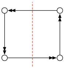
(a) Phase I

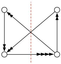
(b) Phase II

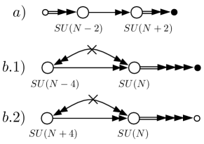
(c) The resulting quiverfolds

Figure 6: 6(a)–6(b) The two Seiberg-dual quiver gauge theories for $\mathbb{F}_{0}$. The red dashed lines indicate orientifold involutions compatible with the $SU(2)\times SU(2)$ isometry of the base. 6(c) The $SU(2)\times SU(2)$-preserving anomaly-free quiverfolds that result from orientifolding these theories.

In the $\mathbb{C}^{3}/\mathbb{Z}_{3}$ and $dP_{1}$ examples studied previously, there was only one toric phase, and we found a duality relating two different orientifolds of that phase which differed by exchanging $SO$ and $U\!Sp$ groups and symmetric and antisymmetric tensor matter, a “negative rank duality” as explained in appendix B. We argue in transitions2 that these dualities relate to the $SL(2,\mathbb{Z})$ self-duality of type IIB string theory. Interestingly, negative rank duality also partly “explains” the pattern of $\mathcal{N}=4$ dualities between $SO$ and $U\!Sp$ theories, suggesting that it may have some physical interpretation relating to Montonen-Olive duality and its $\mathcal{N}=1$ analogues.

By contrast, for the $\mathbb{F}_{0}$ orientifolds we now study, the negative rank duals are either trivially equivalent or related by Seiberg duality. Instead, we find a nontrivial duality between orientifolds of the two different phases. Although the two phases are related by Seiberg duality in the parent theory, the resulting orientifolds are not obviously related in this way, giving yet another new field theory duality.

As in our previous examples, we wish to consider orientifolds corresponding to compact O7 planes wrapping the base $\mathbb{F}_{0}$. This is equivalent to the requirement that the orientifold preserves the $SU(2)\times SU(2)$ isometry of the base. Only the involutions pictured in figure 6(a)–6(b) do so, and of the fixed-element sign choices compatible with $SU(2)\times SU(2)$ invariance, only one choice for phase I and two for phase II lead to anomaly-free theories, giving the theories pictured in figure 6(c).

Notice that the sole orientifold of phase I is its own negative rank dual, whereas the two orientifolds of phase II are related by negative rank duality. As we shall see, the latter two theories are Seiberg dual upon dualizing the left-node. We now discuss the orientifolds of each phase in turn, providing evidence for a duality between the orientifolds of the different phases.

Phase I

We obtain the orientifold theory:

$$\begin{array}[]{c|cc|ccccc}&SU(N-2)&SU(N+2)&SU(2)_{1}&SU(2)_{2}&U(1)_{B}&U(1)_{R}&\mathbb{Z}_{2}\\ \hline\cr A^{i}&\leavevmode\hbox{\vtop{\offinterlineskip\openup-0.4pt\halign{&\startbox@YT{\defarg@YT}{}#\endbox@YT\cr\framebox{\vbox to5.0pt{\vss\hbox to5.0pt{\hss$$\hss}\vss}}\cr}}\kern 5.0pt}&\overline{}\leavevmode\hbox{\vtop{\offinterlineskip\openup-0.4pt\halign{&\startbox@YT{\defarg@YT}{}#\endbox@YT\cr\framebox{\vbox to5.0pt{\vss\hbox to5.0pt{\hss$$\hss}\vss}}\cr}}\kern 5.0pt}&\leavevmode\hbox{\vtop{\offinterlineskip\openup-0.4pt\halign{&\startbox@YT{\defarg@YT}{}#\endbox@YT\cr\framebox{\vbox to5.0pt{\vss\hbox to5.0pt{\hss$$\hss}\vss}}\cr}}\kern 5.0pt}&{\bf 1}&\frac{N}{N^{2}-4}&\frac{1}{2}-\frac{6}{N^{2}-4}&\omega_{2(N-2)}\\ B^{i}&\overline{}\leavevmode\hbox{\vtop{\offinterlineskip\openup-0.4pt\halign{&\startbox@YT{\defarg@YT}{}#\endbox@YT\cr\framebox{\vbox to5.0pt{\vss\hbox to5.0pt{\hss$$\hss}\vss}}&\framebox{\vbox to5.0pt{\vss\hbox to5.0pt{\hss$$\hss}\vss}}\cr}}\kern 10.0pt}&{\bf 1}&{\bf 1}&\leavevmode\hbox{\vtop{\offinterlineskip\openup-0.4pt\halign{&\startbox@YT{\defarg@YT}{}#\endbox@YT\cr\framebox{\vbox to5.0pt{\vss\hbox to5.0pt{\hss$$\hss}\vss}}\cr}}\kern 5.0pt}&-\frac{1}{N-2}&\frac{1}{2}+\frac{3}{N-2}&\omega_{2(N-2)}^{-2}\\ C^{i}&{\bf 1}&\leavevmode\hbox{\vtop{\offinterlineskip\openup-0.4pt\halign{&\startbox@YT{\defarg@YT}{}#\endbox@YT\cr\framebox{\vbox to5.0pt{\vss\hbox to5.0pt{\hss$$\hss}\vss}}\cr\framebox{\vbox to5.0pt{\vss\hbox to5.0pt{\hss$$\hss}\vss}}\cr}}\kern 5.0pt}&{\bf 1}&\leavevmode\hbox{\vtop{\offinterlineskip\openup-0.4pt\halign{&\startbox@YT{\defarg@YT}{}#\endbox@YT\cr\framebox{\vbox to5.0pt{\vss\hbox to5.0pt{\hss$$\hss}\vss}}\cr}}\kern 5.0pt}&-\frac{1}{N+2}&\frac{1}{2}-\frac{3}{N+2}&1\end{array}$$ (450)

with superpotential given by

$$W=\epsilon_{ij}\epsilon_{kl}\mathrm{Tr\,}\left(A^{i}B^{k}A^{j}C^{l}\right)\,.$$ (451)

For odd $N$, the $\mathbb{Z}_{2}$ discrete symmetry is gauge equivalent to the $\mathbb{Z}_{2}$ center of $SU(2)_{1}$, whereas for even $N$ it is a distinct global symmetry. Thus, the global symmetry group is actually $SU(2)_{1}\times SU(2)_{2}\times U(1)_{B}\times U(1)_{R}\times\mathbb{Z}_{\operatorname{gcf}(2,N)}$.

The global anomalies for this theory are shown in table 5(a).

$\begin{array}[]{|c|c|}\hline\cr SU(2)_{1/2}^{3}&(-1)^{N}\\ \hline\cr SU(2)_{1/2}^{2}\,U(1)_{B}&\pm N\\ \hline\cr SU(2)_{1/2}^{2}\,U(1)_{R}&-\tfrac{1}{2}(N^{2}+8)\\ \hline\cr U(1)^{2}_{B}\,U(1)_{R}&-2\\ \hline\cr U(1)_{R}^{3}&\tfrac{3}{2}N^{2}-34\\ \hline\cr U(1)_{R}&-10\\ \hline\cr SU(2)_{1}^{2}\,\mathbb{Z}_{2}&(-1)^{N}\\ \hline\cr SU(2)_{2}^{2}\,\mathbb{Z}_{2}&-(-1)^{N}\\ \hline\cr\mathbb{Z}_{2}&1\\ \hline\cr\end{array}$

(a) Phase I

$\begin{array}[]{|c|c|}\hline\cr SU(2)_{1/2}^{3}&(-1)^{N}\\ \hline\cr SU(2)_{1/2}^{2}\,U(1)_{B}&\pm N\\ \hline\cr SU(2)_{1/2}^{2}\,U(1)_{R}&-\tfrac{1}{2}(N^{2}+8)\\ \hline\cr U(1)^{2}_{B}\,U(1)_{R}&-2\\ \hline\cr U(1)_{R}^{3}&\tfrac{3}{2}N^{2}-34\\ \hline\cr U(1)_{R}&-10\\ \hline\cr SU(2)_{1}^{2}\,\mathbb{Z}_{4}&-1\\ \hline\cr SU(2)_{2}^{2}\,\mathbb{Z}_{4}&-(-1)^{N}\\ \hline\cr\mathbb{Z}_{4}&1\\ \hline\cr\end{array}$

(b) Phase II

Table 5: The nonvanishing anomalies for the orientifolds of the different phases of $\mathbb{F}_{0}$, where we use a multiplicative notation for discrete and Witten anomalies as before (see §3.1). The $U(1)_{B}$, $U(1)_{B}^{3}$, and $U(1)_{B}\,U(1)_{R}^{2}$ anomalies all vanish.

Note that the anomalies are invariant under $N\rightarrow-N$ combined with a charge conjugation of $U(1)_{B}$. This invariance corresponds to taking the negative rank dual as explained in appendix B. While it led to two different gauge theories in the previous examples, one can check that in this case it maps the above theory to itself.

Phase II

We obtain the orientifold theory:

$$\begin{array}[]{c|cc|ccccc}&SU(N-4)&SU(N)&SU(2)_{1}&SU(2)_{2}&U(1)_{B}&U(1)_{R}&\mathbb{Z}_{4}\\ \hline\cr A^{i}&\leavevmode\hbox{\vtop{\offinterlineskip\openup-0.4pt\halign{&\startbox@YT{\defarg@YT}{}#\endbox@YT\cr\framebox{\vbox to5.0pt{\vss\hbox to5.0pt{\hss$$\hss}\vss}}\cr}}\kern 5.0pt}&\overline{}\leavevmode\hbox{\vtop{\offinterlineskip\openup-0.4pt\halign{&\startbox@YT{\defarg@YT}{}#\endbox@YT\cr\framebox{\vbox to5.0pt{\vss\hbox to5.0pt{\hss$$\hss}\vss}}\cr}}\kern 5.0pt}&\leavevmode\hbox{\vtop{\offinterlineskip\openup-0.4pt\halign{&\startbox@YT{\defarg@YT}{}#\endbox@YT\cr\framebox{\vbox to5.0pt{\vss\hbox to5.0pt{\hss$$\hss}\vss}}\cr}}\kern 5.0pt}&{\bf 1}&\frac{1}{N-4}&\frac{1}{2}+\frac{2}{N}&\omega_{4N}^{-1}\,\omega_{4(N-4)}^{-1}\\ B^{i}&\overline{}\leavevmode\hbox{\vtop{\offinterlineskip\openup-0.4pt\halign{&\startbox@YT{\defarg@YT}{}#\endbox@YT\cr\framebox{\vbox to5.0pt{\vss\hbox to5.0pt{\hss$$\hss}\vss}}\cr}}\kern 5.0pt}&\overline{}\leavevmode\hbox{\vtop{\offinterlineskip\openup-0.4pt\halign{&\startbox@YT{\defarg@YT}{}#\endbox@YT\cr\framebox{\vbox to5.0pt{\vss\hbox to5.0pt{\hss$$\hss}\vss}}\cr}}\kern 5.0pt}&{\bf 1}&\leavevmode\hbox{\vtop{\offinterlineskip\openup-0.4pt\halign{&\startbox@YT{\defarg@YT}{}#\endbox@YT\cr\framebox{\vbox to5.0pt{\vss\hbox to5.0pt{\hss$$\hss}\vss}}\cr}}\kern 5.0pt}&-\frac{1}{N-4}&\frac{1}{2}+\frac{2}{N}&\omega_{4N}^{-1}\,\omega_{4(N-4)}\\ C^{i;j}&{\bf 1}&\leavevmode\hbox{\vtop{\offinterlineskip\openup-0.4pt\halign{&\startbox@YT{\defarg@YT}{}#\endbox@YT\cr\framebox{\vbox to5.0pt{\vss\hbox to5.0pt{\hss$$\hss}\vss}}\cr\framebox{\vbox to5.0pt{\vss\hbox to5.0pt{\hss$$\hss}\vss}}\cr}}\kern 5.0pt}&\leavevmode\hbox{\vtop{\offinterlineskip\openup-0.4pt\halign{&\startbox@YT{\defarg@YT}{}#\endbox@YT\cr\framebox{\vbox to5.0pt{\vss\hbox to5.0pt{\hss$$\hss}\vss}}\cr}}\kern 5.0pt}&\leavevmode\hbox{\vtop{\offinterlineskip\openup-0.4pt\halign{&\startbox@YT{\defarg@YT}{}#\endbox@YT\cr\framebox{\vbox to5.0pt{\vss\hbox to5.0pt{\hss$$\hss}\vss}}\cr}}\kern 5.0pt}&0&1-\frac{4}{N}&\omega_{4N}^{2}\end{array}$$ (484)

with superpotential

$$W=\epsilon_{ij}\epsilon_{kj}\mathrm{Tr\,}\left(A^{i}C^{j;k}B^{l}\right),$$ (485)

as well as the theory

$$\begin{array}[]{c|cc|ccccc}&SU(N+4)&SU(N)&SU(2)_{1}&SU(2)_{2}&U(1)_{B}&U(1)_{R}&\mathbb{Z}_{4}\\ \hline\cr\tilde{A}^{i}&\leavevmode\hbox{\vtop{\offinterlineskip\openup-0.4pt\halign{&\startbox@YT{\defarg@YT}{}#\endbox@YT\cr\framebox{\vbox to5.0pt{\vss\hbox to5.0pt{\hss$$\hss}\vss}}\cr}}\kern 5.0pt}&\overline{}\leavevmode\hbox{\vtop{\offinterlineskip\openup-0.4pt\halign{&\startbox@YT{\defarg@YT}{}#\endbox@YT\cr\framebox{\vbox to5.0pt{\vss\hbox to5.0pt{\hss$$\hss}\vss}}\cr}}\kern 5.0pt}&\leavevmode\hbox{\vtop{\offinterlineskip\openup-0.4pt\halign{&\startbox@YT{\defarg@YT}{}#\endbox@YT\cr\framebox{\vbox to5.0pt{\vss\hbox to5.0pt{\hss$$\hss}\vss}}\cr}}\kern 5.0pt}&{\bf 1}&\frac{1}{N+4}&\frac{1}{2}-\frac{2}{N}&\omega_{4N}\,\omega_{4(N+4)}\\ \tilde{B}^{i}&\overline{}\leavevmode\hbox{\vtop{\offinterlineskip\openup-0.4pt\halign{&\startbox@YT{\defarg@YT}{}#\endbox@YT\cr\framebox{\vbox to5.0pt{\vss\hbox to5.0pt{\hss$$\hss}\vss}}\cr}}\kern 5.0pt}&\overline{}\leavevmode\hbox{\vtop{\offinterlineskip\openup-0.4pt\halign{&\startbox@YT{\defarg@YT}{}#\endbox@YT\cr\framebox{\vbox to5.0pt{\vss\hbox to5.0pt{\hss$$\hss}\vss}}\cr}}\kern 5.0pt}&{\bf 1}&\leavevmode\hbox{\vtop{\offinterlineskip\openup-0.4pt\halign{&\startbox@YT{\defarg@YT}{}#\endbox@YT\cr\framebox{\vbox to5.0pt{\vss\hbox to5.0pt{\hss$$\hss}\vss}}\cr}}\kern 5.0pt}&-\frac{1}{N+4}&\frac{1}{2}-\frac{2}{N}&\omega_{4N}\,\omega_{4(N+4)}^{-1}\\ \tilde{C}^{i;j}&{\bf 1}&\leavevmode\hbox{\vtop{\offinterlineskip\openup-0.4pt\halign{&\startbox@YT{\defarg@YT}{}#\endbox@YT\cr\framebox{\vbox to5.0pt{\vss\hbox to5.0pt{\hss$$\hss}\vss}}&\framebox{\vbox to5.0pt{\vss\hbox to5.0pt{\hss$$\hss}\vss}}\cr}}\kern 10.0pt}&\leavevmode\hbox{\vtop{\offinterlineskip\openup-0.4pt\halign{&\startbox@YT{\defarg@YT}{}#\endbox@YT\cr\framebox{\vbox to5.0pt{\vss\hbox to5.0pt{\hss$$\hss}\vss}}\cr}}\kern 5.0pt}&\leavevmode\hbox{\vtop{\offinterlineskip\openup-0.4pt\halign{&\startbox@YT{\defarg@YT}{}#\endbox@YT\cr\framebox{\vbox to5.0pt{\vss\hbox to5.0pt{\hss$$\hss}\vss}}\cr}}\kern 5.0pt}&0&1+\frac{4}{N}&\omega_{4N}^{-2}\end{array}$$ (499)

with superpotential

$$\tilde{W}=\epsilon_{ij}\epsilon_{kj}\mathrm{Tr\,}\left(\tilde{A}^{i}\tilde{C}^{j;k}\tilde{B}^{l}\right).$$ (500)

For odd $N$, the $\mathbb{Z}_{4}$ discrete symmetry is gauge-equivalent to the $\mathbb{Z}_{2}$ center of $SU(2)_{1}$, whereas for $N=4k+2$ the $\mathbb{Z}_{2}\subset\mathbb{Z}_{4}$ subgroup is gauge-equivalent to the $\mathbb{Z}_{2}$ center of $SU(2)_{1}$, and for $N=4k$ the $\mathbb{Z}_{4}$ is a distinct global symmetry. Thus, the global symmetry group is $SU(2)_{1}\times SU(2)_{2}\times U(1)_{B}\times U(1)_{R}\times\mathbb{Z}_{\operatorname{gcf}(4,N)}$.

It is straightforward to check that these two theories, which are related by negative rank duality, are also related by Seiberg dualizing the $SU(N\pm 4)$ gauge group factor and integrating out massive matter.

Relationship between the two phases

The global anomalies for these theories are shown in table 5(b), where for simplicity we do not display the anomalies of the Seiberg dual theories separately; one can verify that they match as expected. More importantly, we see that the phase I and phase II orientifolds have matching anomalies for odd $N_{\text{phase I}}=N_{\text{phase II}}$. For even $N$ the global symmetry groups do not match, and the theories are not dual.

It is interesting to understand better the nature of this prospective duality between orientifolds of the two phases. We will present evidence in transitions3 that the embeddings in string theory for the two phases are related as in realizations of ordinary Seiberg duality, so we can expect the nature of the duality relating the two phases phases to be an infrared duality closely analogous to it. However, we emphasize that this duality is not obviously derivable from known examples of Seiberg duality. In transitions3 , we also argue that the action of IIB S-duality on the D-brane configuration describing each phase reproduces the field theory dualities inside each phase that we just studied: it is a self-duality in phase I and it exchanges the two theories in phase II.

6.3 The real cone over $Y^{4,0}$

Before concluding, we present one final example of new dualities relating the world-volume gauge theories of D3 branes probing a Calabi-Yau singularity. Much like the $\mathbb{F}_{0}$ example studied above, this example exhibits interesting new patterns of dualities which appear distinct from the $\mathbb{C}_{3}/\mathbb{Z}_{3}$ and $dP_{1}$ examples discussed previously.

We consider the real cone over $Y^{4,0}$ which, like the cone over $Y^{2,0}$ considered above, is an orbifold of the conifold. There are five toric quiver gauge theories which describe D3 branes probing this singularity, all of which are Seiberg dual. We focus on the two phases pictured in figure 7 and on the involutions also pictured there.

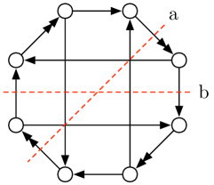
(a) Phase I

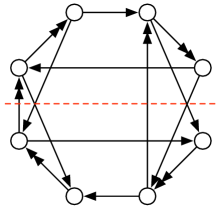
(b) Phase II

Figure 7: Two of the five Seiberg-dual toric quiver gauge theories for $Y^{4,0}$. The red dashed lines indicate the orientifold involutions we will consider.

For simplicity, we restrict our attention to the anomaly-free orientifolds pictured in figure 8. One can show that these orientifolds correspond to compact O7 planes, and preserve the full $SU(2)\times U(1)_{X}\times U(1)_{R}$ isometry group of $Y^{4,0}$. We now briefly discuss each of the three theories in turn, after which we illustrate a potential duality between them using anomaly matching.

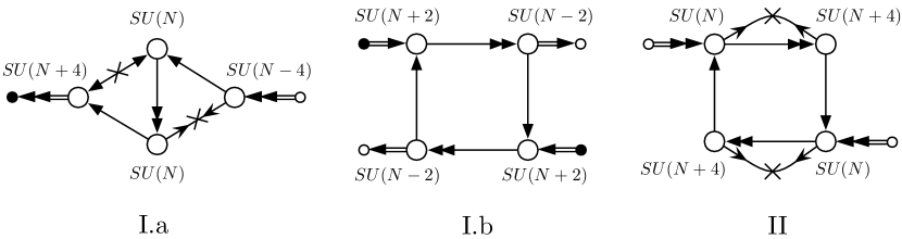
Figure 8: Quiverfolds for the anomaly-free orientifold gauge theories we will consider, arranged by the parent quiver and involution used to generate them (see figure 7). The phase II quiverfold has a negative rank dual which is not pictured, as it is manifestly Seiberg dual to the quiverfold which is shown. The phase I quiverfolds are “self-dual” under negative rank duality.

Phase I, Involution a

We obtain the orientifold theory:

$$\begin{array}[]{c|cccc|cccc}&SU(N+4)&SU(N)&SU(N)&SU(N-4)&SU(2)&U(1)_{B}&U(1)_{X}&U(1)_{R}\\ \hline\cr A^{i}&\leavevmode\hbox{\vtop{\offinterlineskip\openup-0.4pt\halign{&\startbox@YT{\defarg@YT}{}#\endbox@YT\cr\framebox{\vbox to5.0pt{\vss\hbox to5.0pt{\hss$$\hss}\vss}}\cr\framebox{\vbox to5.0pt{\vss\hbox to5.0pt{\hss$$\hss}\vss}}\cr}}\kern 5.0pt}&\mathbf{1}&\mathbf{1}&\mathbf{1}&\leavevmode\hbox{\vtop{\offinterlineskip\openup-0.4pt\halign{&\startbox@YT{\defarg@YT}{}#\endbox@YT\cr\framebox{\vbox to5.0pt{\vss\hbox to5.0pt{\hss$$\hss}\vss}}\cr}}\kern 5.0pt}&\frac{1}{N+4}&0&\frac{1}{2}-\frac{6}{N+4}\\ S^{i}&\mathbf{1}&\mathbf{1}&\mathbf{1}&\overline{}\leavevmode\hbox{\vtop{\offinterlineskip\openup-0.4pt\halign{&\startbox@YT{\defarg@YT}{}#\endbox@YT\cr\framebox{\vbox to5.0pt{\vss\hbox to5.0pt{\hss$$\hss}\vss}}&\framebox{\vbox to5.0pt{\vss\hbox to5.0pt{\hss$$\hss}\vss}}\cr}}\kern 10.0pt}&\leavevmode\hbox{\vtop{\offinterlineskip\openup-0.4pt\halign{&\startbox@YT{\defarg@YT}{}#\endbox@YT\cr\framebox{\vbox to5.0pt{\vss\hbox to5.0pt{\hss$$\hss}\vss}}\cr}}\kern 5.0pt}&\frac{1}{N-4}&0&\frac{1}{2}+\frac{6}{N-4}\\ P_{12}&\overline{}\leavevmode\hbox{\vtop{\offinterlineskip\openup-0.4pt\halign{&\startbox@YT{\defarg@YT}{}#\endbox@YT\cr\framebox{\vbox to5.0pt{\vss\hbox to5.0pt{\hss$$\hss}\vss}}\cr}}\kern 5.0pt}&\overline{}\leavevmode\hbox{\vtop{\offinterlineskip\openup-0.4pt\halign{&\startbox@YT{\defarg@YT}{}#\endbox@YT\cr\framebox{\vbox to5.0pt{\vss\hbox to5.0pt{\hss$$\hss}\vss}}\cr}}\kern 5.0pt}&\mathbf{1}&\mathbf{1}&\mathbf{1}&-\frac{N+2}{N(N+4)}&-\frac{N-4}{N}&\frac{1}{2}+\frac{3}{N+4}\\ P_{13}&\overline{}\leavevmode\hbox{\vtop{\offinterlineskip\openup-0.4pt\halign{&\startbox@YT{\defarg@YT}{}#\endbox@YT\cr\framebox{\vbox to5.0pt{\vss\hbox to5.0pt{\hss$$\hss}\vss}}\cr}}\kern 5.0pt}&\mathbf{1}&\leavevmode\hbox{\vtop{\offinterlineskip\openup-0.4pt\halign{&\startbox@YT{\defarg@YT}{}#\endbox@YT\cr\framebox{\vbox to5.0pt{\vss\hbox to5.0pt{\hss$$\hss}\vss}}\cr}}\kern 5.0pt}&\mathbf{1}&\mathbf{1}&-\frac{N+2}{N(N+4)}&\frac{N-4}{N}&\frac{1}{2}+\frac{3}{N+4}\\ P_{23}^{i}&\mathbf{1}&\leavevmode\hbox{\vtop{\offinterlineskip\openup-0.4pt\halign{&\startbox@YT{\defarg@YT}{}#\endbox@YT\cr\framebox{\vbox to5.0pt{\vss\hbox to5.0pt{\hss$$\hss}\vss}}\cr}}\kern 5.0pt}&\overline{}\leavevmode\hbox{\vtop{\offinterlineskip\openup-0.4pt\halign{&\startbox@YT{\defarg@YT}{}#\endbox@YT\cr\framebox{\vbox to5.0pt{\vss\hbox to5.0pt{\hss$$\hss}\vss}}\cr}}\kern 5.0pt}&\mathbf{1}&\leavevmode\hbox{\vtop{\offinterlineskip\openup-0.4pt\halign{&\startbox@YT{\defarg@YT}{}#\endbox@YT\cr\framebox{\vbox to5.0pt{\vss\hbox to5.0pt{\hss$$\hss}\vss}}\cr}}\kern 5.0pt}&\frac{1}{N}&0&\frac{1}{2}\\ P_{24}&\mathbf{1}&\overline{}\leavevmode\hbox{\vtop{\offinterlineskip\openup-0.4pt\halign{&\startbox@YT{\defarg@YT}{}#\endbox@YT\cr\framebox{\vbox to5.0pt{\vss\hbox to5.0pt{\hss$$\hss}\vss}}\cr}}\kern 5.0pt}&\mathbf{1}&\leavevmode\hbox{\vtop{\offinterlineskip\openup-0.4pt\halign{&\startbox@YT{\defarg@YT}{}#\endbox@YT\cr\framebox{\vbox to5.0pt{\vss\hbox to5.0pt{\hss$$\hss}\vss}}\cr}}\kern 5.0pt}&\mathbf{1}&-\frac{N-2}{N(N-4)}&\frac{N+4}{N}&\frac{1}{2}-\frac{3}{N-4}\\ P_{34}&\mathbf{1}&\mathbf{1}&\leavevmode\hbox{\vtop{\offinterlineskip\openup-0.4pt\halign{&\startbox@YT{\defarg@YT}{}#\endbox@YT\cr\framebox{\vbox to5.0pt{\vss\hbox to5.0pt{\hss$$\hss}\vss}}\cr}}\kern 5.0pt}&\leavevmode\hbox{\vtop{\offinterlineskip\openup-0.4pt\halign{&\startbox@YT{\defarg@YT}{}#\endbox@YT\cr\framebox{\vbox to5.0pt{\vss\hbox to5.0pt{\hss$$\hss}\vss}}\cr}}\kern 5.0pt}&\mathbf{1}&-\frac{N-2}{N(N-4)}&-\frac{N+4}{N}&\frac{1}{2}-\frac{3}{N-4}\end{array}$$ (525)

with superpotential

$$W=\epsilon_{ij}A^{i}P_{12}P_{23}^{j}P_{13}+\epsilon_{ij}S^{i}P_{24}P_{23}^{j}P_{34}\,,$$ (526)

where there is an additional discrete $\mathbb{Z}_{\operatorname{gcf}(4,N)}$ symmetry for even $N$, which we omit from the charge table for simplicity, as it will not play a large role in our analysis.

Phase I, Involution b

We obtain the orientifold theory:

$$\begin{array}[]{c|cccc|cccc}&SU(N+2)&SU(N-2)&SU(N+2)&SU(N-2)&SU(2)&U(1)_{B}&U(1)_{X}&U(1)_{R}\\ \hline\cr T_{1}&\overline{}\leavevmode\hbox{\vtop{\offinterlineskip\openup-0.4pt\halign{&\startbox@YT{\defarg@YT}{}#\endbox@YT\cr\framebox{\vbox to5.0pt{\vss\hbox to5.0pt{\hss$$\hss}\vss}}\cr\framebox{\vbox to5.0pt{\vss\hbox to5.0pt{\hss$$\hss}\vss}}\cr}}\kern 5.0pt}&\mathbf{1}&\mathbf{1}&\mathbf{1}&\mathbf{1}&-\frac{1}{N+2}&\frac{N+4}{N+2}&\frac{1}{2}-\frac{7}{N+2}\\ T_{2}&\mathbf{1}&\leavevmode\hbox{\vtop{\offinterlineskip\openup-0.4pt\halign{&\startbox@YT{\defarg@YT}{}#\endbox@YT\cr\framebox{\vbox to5.0pt{\vss\hbox to5.0pt{\hss$$\hss}\vss}}&\framebox{\vbox to5.0pt{\vss\hbox to5.0pt{\hss$$\hss}\vss}}\cr}}\kern 10.0pt}&\mathbf{1}&\mathbf{1}&\mathbf{1}&-\frac{1}{N-2}&-\frac{N-4}{N-2}&\frac{1}{2}+\frac{7}{N-2}\\ T_{3}&\mathbf{1}&\mathbf{1}&\overline{}\leavevmode\hbox{\vtop{\offinterlineskip\openup-0.4pt\halign{&\startbox@YT{\defarg@YT}{}#\endbox@YT\cr\framebox{\vbox to5.0pt{\vss\hbox to5.0pt{\hss$$\hss}\vss}}\cr\framebox{\vbox to5.0pt{\vss\hbox to5.0pt{\hss$$\hss}\vss}}\cr}}\kern 5.0pt}&\mathbf{1}&\mathbf{1}&-\frac{1}{N+2}&-\frac{N+4}{N+2}&\frac{1}{2}-\frac{7}{N+2}\\ T_{4}&\mathbf{1}&\mathbf{1}&\mathbf{1}&\leavevmode\hbox{\vtop{\offinterlineskip\openup-0.4pt\halign{&\startbox@YT{\defarg@YT}{}#\endbox@YT\cr\framebox{\vbox to5.0pt{\vss\hbox to5.0pt{\hss$$\hss}\vss}}&\framebox{\vbox to5.0pt{\vss\hbox to5.0pt{\hss$$\hss}\vss}}\cr}}\kern 10.0pt}&\mathbf{1}&-\frac{1}{N-2}&\frac{N-4}{N-2}&\frac{1}{2}+\frac{7}{N-2}\\ P_{12}^{i}&\leavevmode\hbox{\vtop{\offinterlineskip\openup-0.4pt\halign{&\startbox@YT{\defarg@YT}{}#\endbox@YT\cr\framebox{\vbox to5.0pt{\vss\hbox to5.0pt{\hss$$\hss}\vss}}\cr}}\kern 5.0pt}&\overline{}\leavevmode\hbox{\vtop{\offinterlineskip\openup-0.4pt\halign{&\startbox@YT{\defarg@YT}{}#\endbox@YT\cr\framebox{\vbox to5.0pt{\vss\hbox to5.0pt{\hss$$\hss}\vss}}\cr}}\kern 5.0pt}&\mathbf{1}&\mathbf{1}&\leavevmode\hbox{\vtop{\offinterlineskip\openup-0.4pt\halign{&\startbox@YT{\defarg@YT}{}#\endbox@YT\cr\framebox{\vbox to5.0pt{\vss\hbox to5.0pt{\hss$$\hss}\vss}}\cr}}\kern 5.0pt}&\frac{N}{N^{2}-4}&-\frac{2N}{N^{2}-4}&\frac{1}{2}-\frac{14}{N^{2}-4}\\ P_{23}&\mathbf{1}&\leavevmode\hbox{\vtop{\offinterlineskip\openup-0.4pt\halign{&\startbox@YT{\defarg@YT}{}#\endbox@YT\cr\framebox{\vbox to5.0pt{\vss\hbox to5.0pt{\hss$$\hss}\vss}}\cr}}\kern 5.0pt}&\overline{}\leavevmode\hbox{\vtop{\offinterlineskip\openup-0.4pt\halign{&\startbox@YT{\defarg@YT}{}#\endbox@YT\cr\framebox{\vbox to5.0pt{\vss\hbox to5.0pt{\hss$$\hss}\vss}}\cr}}\kern 5.0pt}&\mathbf{1}&\mathbf{1}&-\frac{N}{N^{2}-4}&\frac{N^{2}}{N^{2}-4}&\frac{1}{2}+\frac{14}{N^{2}-4}\\ P_{34}^{i}&\mathbf{1}&\mathbf{1}&\leavevmode\hbox{\vtop{\offinterlineskip\openup-0.4pt\halign{&\startbox@YT{\defarg@YT}{}#\endbox@YT\cr\framebox{\vbox to5.0pt{\vss\hbox to5.0pt{\hss$$\hss}\vss}}\cr}}\kern 5.0pt}&\overline{}\leavevmode\hbox{\vtop{\offinterlineskip\openup-0.4pt\halign{&\startbox@YT{\defarg@YT}{}#\endbox@YT\cr\framebox{\vbox to5.0pt{\vss\hbox to5.0pt{\hss$$\hss}\vss}}\cr}}\kern 5.0pt}&\leavevmode\hbox{\vtop{\offinterlineskip\openup-0.4pt\halign{&\startbox@YT{\defarg@YT}{}#\endbox@YT\cr\framebox{\vbox to5.0pt{\vss\hbox to5.0pt{\hss$$\hss}\vss}}\cr}}\kern 5.0pt}&\frac{N}{N^{2}-4}&\frac{2N}{N^{2}-4}&\frac{1}{2}-\frac{14}{N^{2}-4}\\ P_{41}&\overline{}\leavevmode\hbox{\vtop{\offinterlineskip\openup-0.4pt\halign{&\startbox@YT{\defarg@YT}{}#\endbox@YT\cr\framebox{\vbox to5.0pt{\vss\hbox to5.0pt{\hss$$\hss}\vss}}\cr}}\kern 5.0pt}&\mathbf{1}&\mathbf{1}&\leavevmode\hbox{\vtop{\offinterlineskip\openup-0.4pt\halign{&\startbox@YT{\defarg@YT}{}#\endbox@YT\cr\framebox{\vbox to5.0pt{\vss\hbox to5.0pt{\hss$$\hss}\vss}}\cr}}\kern 5.0pt}&\mathbf{1}&-\frac{N}{N^{2}-4}&-\frac{N^{2}}{N^{2}-4}&\frac{1}{2}+\frac{14}{N^{2}-4}\end{array}$$ (552)

with superpotential

$$W=\frac{1}{2}\epsilon_{ij}T_{1}P_{12}^{i}P_{12}^{j}T_{2}+\frac{1}{2}\epsilon_{ij}T_{3}P_{34}^{i}P_{34}^{j}T_{4}+\epsilon_{ij}P_{12}^{i}P_{23}P_{34}^{j}P_{41}\,.$$ (553)

As before, there is an additional discrete $\mathbb{Z}_{\operatorname{gcf}(4,N)}$ symmetry for even $N$.

Phase II

We obtain the orientifold theory:

$$\begin{array}[]{c|cccc|cccc}&SU(N+4)&SU(N)&SU(N+4)&SU(N)&SU(2)&U(1)_{B}&U(1)_{X}&U(1)_{R}\\ \hline\cr P_{12}&\leavevmode\hbox{\vtop{\offinterlineskip\openup-0.4pt\halign{&\startbox@YT{\defarg@YT}{}#\endbox@YT\cr\framebox{\vbox to5.0pt{\vss\hbox to5.0pt{\hss$$\hss}\vss}}\cr}}\kern 5.0pt}&\overline{}\leavevmode\hbox{\vtop{\offinterlineskip\openup-0.4pt\halign{&\startbox@YT{\defarg@YT}{}#\endbox@YT\cr\framebox{\vbox to5.0pt{\vss\hbox to5.0pt{\hss$$\hss}\vss}}\cr}}\kern 5.0pt}&\mathbf{1}&\mathbf{1}&\mathbf{1}&-\frac{1}{N+4}&-\frac{N+2}{N+4}&\frac{1}{2}+\frac{2(N+8)}{N(N+4)}\\ P_{23}&\mathbf{1}&\leavevmode\hbox{\vtop{\offinterlineskip\openup-0.4pt\halign{&\startbox@YT{\defarg@YT}{}#\endbox@YT\cr\framebox{\vbox to5.0pt{\vss\hbox to5.0pt{\hss$$\hss}\vss}}\cr}}\kern 5.0pt}&\leavevmode\hbox{\vtop{\offinterlineskip\openup-0.4pt\halign{&\startbox@YT{\defarg@YT}{}#\endbox@YT\cr\framebox{\vbox to5.0pt{\vss\hbox to5.0pt{\hss$$\hss}\vss}}\cr}}\kern 5.0pt}&\mathbf{1}&\mathbf{1}&-\frac{1}{N+4}&-\frac{N+6}{N+4}&\frac{1}{2}-\frac{2(3N+8)}{N(N+4)}\\ P_{34}&\mathbf{1}&\mathbf{1}&\leavevmode\hbox{\vtop{\offinterlineskip\openup-0.4pt\halign{&\startbox@YT{\defarg@YT}{}#\endbox@YT\cr\framebox{\vbox to5.0pt{\vss\hbox to5.0pt{\hss$$\hss}\vss}}\cr}}\kern 5.0pt}&\overline{}\leavevmode\hbox{\vtop{\offinterlineskip\openup-0.4pt\halign{&\startbox@YT{\defarg@YT}{}#\endbox@YT\cr\framebox{\vbox to5.0pt{\vss\hbox to5.0pt{\hss$$\hss}\vss}}\cr}}\kern 5.0pt}&\mathbf{1}&-\frac{1}{N+4}&\frac{N+2}{N+4}&\frac{1}{2}+\frac{2(N+8)}{N(N+4)}\\ P_{41}&\leavevmode\hbox{\vtop{\offinterlineskip\openup-0.4pt\halign{&\startbox@YT{\defarg@YT}{}#\endbox@YT\cr\framebox{\vbox to5.0pt{\vss\hbox to5.0pt{\hss$$\hss}\vss}}\cr}}\kern 5.0pt}&\mathbf{1}&\mathbf{1}&\leavevmode\hbox{\vtop{\offinterlineskip\openup-0.4pt\halign{&\startbox@YT{\defarg@YT}{}#\endbox@YT\cr\framebox{\vbox to5.0pt{\vss\hbox to5.0pt{\hss$$\hss}\vss}}\cr}}\kern 5.0pt}&\mathbf{1}&-\frac{1}{N+4}&\frac{N+6}{N+4}&\frac{1}{2}-\frac{2(3N+8)}{N(N+4)}\\ X_{2}^{i}&\mathbf{1}&\overline{}\leavevmode\hbox{\vtop{\offinterlineskip\openup-0.4pt\halign{&\startbox@YT{\defarg@YT}{}#\endbox@YT\cr\framebox{\vbox to5.0pt{\vss\hbox to5.0pt{\hss$$\hss}\vss}}&\framebox{\vbox to5.0pt{\vss\hbox to5.0pt{\hss$$\hss}\vss}}\cr}}\kern 10.0pt}&\mathbf{1}&\mathbf{1}&\leavevmode\hbox{\vtop{\offinterlineskip\openup-0.4pt\halign{&\startbox@YT{\defarg@YT}{}#\endbox@YT\cr\framebox{\vbox to5.0pt{\vss\hbox to5.0pt{\hss$$\hss}\vss}}\cr}}\kern 5.0pt}&0&1&1+\frac{8}{N}\\ X_{4}^{i}&\mathbf{1}&\mathbf{1}&\mathbf{1}&\overline{}\leavevmode\hbox{\vtop{\offinterlineskip\openup-0.4pt\halign{&\startbox@YT{\defarg@YT}{}#\endbox@YT\cr\framebox{\vbox to5.0pt{\vss\hbox to5.0pt{\hss$$\hss}\vss}}&\framebox{\vbox to5.0pt{\vss\hbox to5.0pt{\hss$$\hss}\vss}}\cr}}\kern 10.0pt}&\leavevmode\hbox{\vtop{\offinterlineskip\openup-0.4pt\halign{&\startbox@YT{\defarg@YT}{}#\endbox@YT\cr\framebox{\vbox to5.0pt{\vss\hbox to5.0pt{\hss$$\hss}\vss}}\cr}}\kern 5.0pt}&0&-1&1+\frac{8}{N}\\ T_{41}^{i}&\overline{}\leavevmode\hbox{\vtop{\offinterlineskip\openup-0.4pt\halign{&\startbox@YT{\defarg@YT}{}#\endbox@YT\cr\framebox{\vbox to5.0pt{\vss\hbox to5.0pt{\hss$$\hss}\vss}}\cr}}\kern 5.0pt}&\mathbf{1}&\mathbf{1}&\leavevmode\hbox{\vtop{\offinterlineskip\openup-0.4pt\halign{&\startbox@YT{\defarg@YT}{}#\endbox@YT\cr\framebox{\vbox to5.0pt{\vss\hbox to5.0pt{\hss$$\hss}\vss}}\cr}}\kern 5.0pt}&\leavevmode\hbox{\vtop{\offinterlineskip\openup-0.4pt\halign{&\startbox@YT{\defarg@YT}{}#\endbox@YT\cr\framebox{\vbox to5.0pt{\vss\hbox to5.0pt{\hss$$\hss}\vss}}\cr}}\kern 5.0pt}&\frac{1}{N+4}&-\frac{2}{N+4}&\frac{1}{2}-\frac{2(N+8)}{N(N+4)}\\ T_{23}^{i}&\mathbf{1}&\leavevmode\hbox{\vtop{\offinterlineskip\openup-0.4pt\halign{&\startbox@YT{\defarg@YT}{}#\endbox@YT\cr\framebox{\vbox to5.0pt{\vss\hbox to5.0pt{\hss$$\hss}\vss}}\cr}}\kern 5.0pt}&\overline{}\leavevmode\hbox{\vtop{\offinterlineskip\openup-0.4pt\halign{&\startbox@YT{\defarg@YT}{}#\endbox@YT\cr\framebox{\vbox to5.0pt{\vss\hbox to5.0pt{\hss$$\hss}\vss}}\cr}}\kern 5.0pt}&\mathbf{1}&\leavevmode\hbox{\vtop{\offinterlineskip\openup-0.4pt\halign{&\startbox@YT{\defarg@YT}{}#\endbox@YT\cr\framebox{\vbox to5.0pt{\vss\hbox to5.0pt{\hss$$\hss}\vss}}\cr}}\kern 5.0pt}&\frac{1}{N+4}&\frac{2}{N+4}&\frac{1}{2}-\frac{2(N+8)}{N(N+4)}\end{array}$$ (581)

with superpotential

$$W=\epsilon_{ij}X_{2}^{i}P_{23}T_{23}^{j}+\epsilon_{ij}X_{4}^{i}P_{41}T_{41}^{j}+\epsilon_{ij}P_{12}T_{23}^{i}P_{34}T_{41}^{j}\,.$$ (582)

In this case, there is an additional discrete $\mathbb{Z}_{\mathrm{gcf}(8,N)}$ symmetry for even $N$.

Relationship between the different orientifolds

One can show that the anomalies involving the continuous global symmetries match between all three theories considered above, where the nonvanishing anomalies (excluding discrete anomalies) are shown in table 6.

$$\begin{array}[]{|c|c|}\hline\cr SU(2)^{2}\,U(1)_{B}&2N\\ \hline\cr U(1)_{X}^{2}\,U(1)_{B}&-4N\\ \hline\cr SU(2)^{2}\,U(1)_{R}&-N^{2}-24\\ \hline\cr U(1)^{2}_{B}\,U(1)_{R}&-4\\ \hline\cr U(1)^{2}_{X}\,U(1)_{R}&-2(N^{2}+32)\\ \hline\cr U(1)_{R}^{3}&3N^{2}-164\\ \hline\cr U(1)_{R}&-20\\ \hline\cr\end{array}$$

Table 6: The nonvanishing anomalies of the three different $Y^{4,0}$ theories. We omit discrete anomalies for simplicity, as there are no discrete symmetries for odd $N$, whereas we argue that no dualities are possible for even $N$.

For odd $N$ there are no discrete symmetries and therefore all three theories have matching global symmetry groups and anomalies. For even $N$ not divisible by eight, the global symmetry groups again match between all three theories. However, by removing $k$ D3 branes we can reduce $N\to N-2k$. Thus, consistency along the Coulomb branch rules out a duality between phase I and phase II for even $N$, since $\mathbb{Z}_{\mathrm{gcf}(8,N)}\neq\mathbb{Z}_{\mathrm{gcf}(4,N)}$ for $N=8p$.

This leaves open the possibility of a duality between the two orientifolds of phase I for even $N$. However, one can show that the operator spectra do not match in this case. Specifically, we can compare the baryons of minimum R-charge in both theories:

I.a I.b Baryon $$A^{\frac{N+4}{2}} T_{1}^{\frac{N+2}{2}} T_{3}^{\frac{N+2}{2}} Q_{B} 1/2 -1/2 Q_{X} 0 \frac{N+4}{2} -\frac{N+4}{2} Q_{R} \frac{N}{4}-2 \frac{N}{4}-3$$ or or (588)

Clearly the operators do not match each other, which is inconsistent with a duality between these two theories for even $N$. Moreover, in the phase II theory only integral $Q_{B}$ is possible, so these operators have no dual there either, consistent with the mismatch in discrete symmetries explained above. Thus, we conclude that there are no dualities between the different theories for even $N$.

For odd $N$, these issues do not arise, as the above operators are no longer well-defined, and only integral $Q_{B}$ is possible in all three theories. As an additional check that a duality can occur for this case, we again consider the baryons of minimal R-charge. For theory I.a, we find the baryons $P_{24}^{N-4}P_{12}^{4}A^{2}$ and $P_{34}^{N-4}P_{13}^{4}A^{2}$, which transform as $\left(\leavevmode\hbox{\vtop{\offinterlineskip\openup-0.4pt\halign{&\startbox@YT{\defarg@YT}{}#\endbox@YT\cr\framebox{\vbox to5.0pt{\vss\hbox to5.0pt{\hss$$\hss}\vss}}&\framebox{\vbox to5.0pt{\vss\hbox to5.0pt{\hss$$\hss}\vss}}\cr}}\kern 10.0pt},-1,\pm(N-4),\frac{N-4}{2}\right)$ under $SU(2)\times U(1)_{B}\times U(1)_{X}\times U(1)_{R}$. Consistent with the proposed duality, we find that the theory I.b baryons $T_{1}^{N}(T_{3}P_{34}^{2}P_{41}^{2})^{2}$ and $T_{3}^{N}(T_{1}P_{12}^{2}P_{23}^{2})^{2}$ have the same charges under the global symmetries, as do the theory II baryons $P_{41}^{N}(P_{12}^{2}P_{23}T_{23})^{2}$ and $P_{23}^{N}(P_{34}^{2}P_{41}T_{41})^{2}$, where the F-term conditions play a nontrivial role in the latter two cases.

The duality between the two orientifolds of phase I is an intriguing new feature of this geometry which does not appear in the simpler examples we considered previously. We leave further discussion of it to a future work.

7 Conclusions

In this paper, we showed that the $\mathcal{N}=1$ gauge theories arising on D3 branes probing orientifolded Calabi-Yau singularities exhibit a rich class of gauge theory dualities not previously explored in the literature. We focused on a particular example of these dualities, corresponding to the well-known $\mathbb{C}_{3}/\mathbb{Z}_{3}$ singularity, providing extensive checks for the proposed duality, including anomaly matching, matching of discrete symmetries, moduli space matching, and matching of the superconformal indices. In some instances the matching of various quantities between the two theories follows from, or would imply, some remarkable mathematical identities, see for example appendices F and G. Together, the success of these checks presents a compelling argument for the existence of a duality.

In transitions3 , we argue that this duality originates from the $SL(2,\mathbb{Z})$ self-duality of type IIB string theory, and is therefore a close cousin of the more familiar Montonen-Olive duality of $\mathcal{N}=4$ theories. In §3.2 we show that $SL(2,\mathbb{Z})$ then acts in the usual way on a particular combination of holomorphic couplings which is constant along the RG flow and which corresponds to the axio-dilaton of type IIB string theory. We conclude that the dual descriptions we find are different weakly coupled limits of a single theory — the theory of branes at the orientifolded singularity — valid for complementary ranges of axio-dilaton vevs. These features make it clear that this $\mathcal{N}=1$ duality is of a different type than the more usually considered Seiberg (infrared) duality. Rather, it is more closely analogous to Montonen-Olive duality, differing only by the reduced supersymmetry and consequently richer dynamics.

As the axio-dilaton corresponds to a holomorphic combination of couplings which is RGE invariant, in general these theories will flow to a complex fixed line parameterized by the axio-dilaton. (We have demonstrated that this occurs in a specific example where part of the fixed line is perturbatively accessible.) The $SL(2,\mathbb{Z})$ duality group therefore acts nontrivially on the fixed line, much as in the $\mathcal{N}=1^{*}$ theories already understood in the literature Leigh:1995ep ; Argyres:1999xu , which are mass deformations of $\mathcal{N}=2$ or $\mathcal{N}=4$ theories and inherit their $SL(2,\mathbb{Z})$ duality directly from that of the parent theory. In certain special cases, however, the flows corresponding to different values of the string coupling converge to a single fixed point. In these cases, one of which we discuss in the text, the $SL(2,\mathbb{Z})$ duality gives rise to an infrared duality relating the two dual theories, both taken at weak string coupling as in ordinary Seiberg duality.

The orientifolded $\mathbb{C}_{3}/\mathbb{Z}_{3}$ singularity is but one example among many geometries that exhibit these dualities. We expect that D3 branes probing any orientifolded Calabi-Yau singularity will exhibit an $SL(2,\mathbb{Z})$ duality so long as the O7 planes are compact, though in some cases it is only a self-duality. For example, the $dP_{1}$ singularity is a closely related geometry giving rise to a dual pair of gauge theories related to the $\mathbb{C}^{3}/\mathbb{Z}_{3}$ theories by Higgsing (corresponding to blowing down a two-cycle in the $dP_{1}$ base). These theories exhibit interesting dynamics, such as a quantum-deformed moduli space for the lowest rank example which we were able to completely match between the dual theories. It would be interesting to understand the dynamics of these theories for larger $N$. In transitions2 ; transitions3 we provide infinite classes of geometries which generalize $\mathbb{C}_{3}/\mathbb{Z}_{3}$ and $dP_{1}$, all of which exhibit similar dualities.

In addition to $SL(2,\mathbb{Z})$ dualities, more complicated geometries (such as the $\mathbb{F}_{0}$ singularity) also exhibit other interesting dualities. The simplest of these appear to be closely related to Seiberg duality, at least from the perspective of string theory, as we argue in transitions3 . However, from the field theory perspective, they are new (presumably infrared) dualities not readily derivable from the Seiberg duals known in the literature. We also find indications of further dualities whose string theoretic origin is unclear, such as the duality relating the two orientifolds of phase I of $Y^{4,0}$. It would be interesting to better understand the nature and origin of these dualities.

We anticipate that further study of these dualities will lead to new insights concerning both string theory and gauge theories. In particular, on the gauge theory side, our work helps to substantially expand the universe of known dualities to cases where product gauge groups play a pivotal role, and radically broadens the contexts in which $SL(2,\mathbb{Z})$ dualities are seen to arise. The infinite variety of Calabi-Yau singularities provides plenty of room for further study, which could reveal further types of duality or further illuminate the dualities we have considered here.

Finally, given a clear understanding of when dualities are expected to occur in string theory, it might be possible to construct examples of $\mathcal{N}=0$ dualities. Indeed, this has recently been attempted for the case where supersymmetry is broken by antibranes Sugimoto:2012rt . Our work suggests a related program of dualities from anti-branes at Calabi-Yau singularities, or from branes probing SUSY-breaking singularities, such as non-supersymmetric orbifolds. While string theory seems to suggest that both cases should lead to $SL(2,\mathbb{Z})$ dualities, this seems extraordinary from the field theory perspective, making it a natural topic for further research.

Appendix A Quiverfolds

As the main focus of our paper is dualities relating gauge theories arising on the worldvolumes of D3 branes probing orientifolded Calabi-Yau singularities, it is useful to establish some general facts about these gauge theories.

While D-brane gauge theories are quiver gauge theories, the introduction of O-planes leads to a slightly more general class of theories which we refer to as “quiverfold” gauge theories. Quiverfold gauge theories admit more general gauge groups and matter content than quiver gauge theories. While quiver gauge theories allow only $SU$ gauge group factors as well as adjoint and bifundamental $(\leavevmode\hbox{\vtop{\offinterlineskip\openup-0.4pt\halign{&\startbox@YT{\defarg@YT}{}#\endbox@YT\cr\framebox{\vbox to5.0pt{\vss\hbox to5.0pt{\hss$$\hss}\vss}}\cr}}\kern 5.0pt},\overline{}\leavevmode\hbox{\vtop{\offinterlineskip\openup-0.4pt\halign{&\startbox@YT{\defarg@YT}{}#\endbox@YT\cr\framebox{\vbox to5.0pt{\vss\hbox to5.0pt{\hss$$\hss}\vss}}\cr}}\kern 5.0pt})$ or $(\overline{}\leavevmode\hbox{\vtop{\offinterlineskip\openup-0.4pt\halign{&\startbox@YT{\defarg@YT}{}#\endbox@YT\cr\framebox{\vbox to5.0pt{\vss\hbox to5.0pt{\hss$$\hss}\vss}}\cr}}\kern 5.0pt},\leavevmode\hbox{\vtop{\offinterlineskip\openup-0.4pt\halign{&\startbox@YT{\defarg@YT}{}#\endbox@YT\cr\framebox{\vbox to5.0pt{\vss\hbox to5.0pt{\hss$$\hss}\vss}}\cr}}\kern 5.0pt})$ matter, quiverfold gauge theories also allow $SO$ and $U\!Sp$ groups, as well as two-index tensor matter and bifundamental matter in the $(\leavevmode\hbox{\vtop{\offinterlineskip\openup-0.4pt\halign{&\startbox@YT{\defarg@YT}{}#\endbox@YT\cr\framebox{\vbox to5.0pt{\vss\hbox to5.0pt{\hss$$\hss}\vss}}\cr}}\kern 5.0pt},\leavevmode\hbox{\vtop{\offinterlineskip\openup-0.4pt\halign{&\startbox@YT{\defarg@YT}{}#\endbox@YT\cr\framebox{\vbox to5.0pt{\vss\hbox to5.0pt{\hss$$\hss}\vss}}\cr}}\kern 5.0pt})$ or $(\overline{}\leavevmode\hbox{\vtop{\offinterlineskip\openup-0.4pt\halign{&\startbox@YT{\defarg@YT}{}#\endbox@YT\cr\framebox{\vbox to5.0pt{\vss\hbox to5.0pt{\hss$$\hss}\vss}}\cr}}\kern 5.0pt},\overline{}\leavevmode\hbox{\vtop{\offinterlineskip\openup-0.4pt\halign{&\startbox@YT{\defarg@YT}{}#\endbox@YT\cr\framebox{\vbox to5.0pt{\vss\hbox to5.0pt{\hss$$\hss}\vss}}\cr}}\kern 5.0pt})$ representations.

Such gauge theories cannot be described by standard quiver diagrams (directed graphs), and we develop a more general diagrammatic notation in §A.3, which we call a “quiverfold diagram”. One can show that any connected quiverfold diagram which is not a strict quiver can be thought of (in a precise way which we later make clear) as the result of “folding” a quiver in half along a line of $\mathbb{Z}_{2}$ symmetry, which is the inspiration for the term “quiverfold”.

Before discussing quiverfolds in §A.3, we first motivate their introduction by “deriving” a set of rules for obtaining orientifold gauge theories from their parent (orientifold-free) quiver gauge theory in §A.1 and applying these rules to a few simple examples in §A.2. As shown in transitions3 , these rules are equivalent to well-established results in the literature on orientifolding toric Calabi-Yau singularities using brane tilings Franco:2007ii . While the brane tiling method has some computational advantages relating to the superpotential, our approach (following Wijnholt:2007vn ) is somewhat more intuitive, and we focus on it here for that reason, deferring further discussion of brane tiling methods to transitions3 .

A.1 Orientifolding a quiver gauge theory

We consider a quiver gauge theory describing a collection of D-branes probing some background. Each node in the quiver corresponds to a stack of identical D-branes, with an associated $U(N)$ gauge group. Arrows in the quiver, bifundamental matter in the quiver gauge theory, correspond to open strings stretched between the stacks of branes at their intersections.

To this picture, we now add orientifold planes (O-planes). The associated involution, $\sigma$, must map the background and the collection of branes onto itself (up to certain signs and orientations), and squares to the identity. Thus, the involution defines an order-two permutation on the nodes of the quiver. Moreover, the involution maps open strings to oppositely oriented open strings. Thus, the involution also defines an order-two permutation on the arrows of the quiver, such that for any arrow $X:A\to B$ connecting node $A$ to node $B$, the arrow’s orientifold image $X^{\prime}:B^{\prime}\to A^{\prime}$ connects $B^{\prime}$ to $A^{\prime}$, where $A^{\prime}$ and $B^{\prime}$ are the orientifold images of the nodes $A$ and $B$, respectively.

The observations of the last paragraph may be summarized as follows:

Rule I: The O-plane involution defines a $\mathbb{Z}_{2}$ automorphism of the quiver which reverses the directions of arrows.

An example of the resulting involution is shown in figure 9. Note that not every quiver has an involution, in the sense defined above. A necessary condition is that the quiver be isomorphic to its charge conjugate (the same quiver with the arrows reversed). This corresponds to the fact that not all brane configurations can be orientifolded, since the branes must then come in image pairs under the involution.

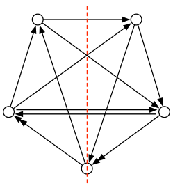
Figure 9: An example of an involution of a quiver. The quiver theory pictured here describes the toric $PdP_{2}$ singularity Feng:2004uq .

D-brane gauge theories generically come with a classical (tree-level) superpotential, which is determined by the geometry and brane configuration. Since these objects are appropriately covariant under the involution, we conclude that the superpotential must also be appropriately covariant: that is, $W\to W^{\prime}$, where $W^{\prime}$ is equivalent to $W$ up to some symmetry transformation. In the examples which follow, we shall see that the appropriate restriction is in fact:

Rule II: The superpotential of the parent theory is invariant under the involution.

Notice that if we impose the same requirement on the (generally unknown) Kähler potential, this implies that the corresponding gauge theory has a color-conjugation symmetry. The orientifold theory results from identifying the chiral and vector superfields related by the involution. This can be restated as:

Rule III: The orientifold gauge theory is derived from the parent theory by gauging the involution.

Note that the above rules should only be interpreted at the classical level. For instance, the gauge group ranks compatible with anomaly cancellation are generally different in the parent and orientifold theories, corresponding to the tadpoles (RR charge) carried by the O-planes.

We have presented a heuristic argument (following Wijnholt:2007vn ) for a set of rules relating the worldvolume theories of stacks of D-branes to the worldvolume gauge theories of their orientifolds. To the extent that these arguments hold, the above rules should be viewed as necessary (but potentially insufficient) conditions which must be satisfied by consistent orientifold involutions. We now illustrate these arguments with a pair of examples.

A.2 Examples

A.2.1 $\mathcal{N}=4$ orientifolds

We consider the worldvolume gauge theory of $N$ parallel D3 branes in flat space, which is $\mathcal{N}=4$ $SU(N)$ super-Yang-Mills. This theory has an $\mathcal{N}=1$ description with three adjoint chiral superfields $\Phi^{i}$, $i\in\{1,2,3\}$, and the superpotential:

$$W=\frac{1}{3}\,\epsilon_{ijk}\mathrm{Tr\,}\Phi^{i}\Phi^{j}\Phi^{k}\,,$$ (598)

up to a superpotential coupling which can be removed by rescaling the fields. However, in this language only an $SU(3)\times U(1)_{R}$ subgroup of the $SU(4)_{R}$ symmetry is manifest, where $\Phi^{i}$ transforms as $\leavevmode\hbox{\vtop{\offinterlineskip\openup-0.4pt\halign{&\startbox@YT{\defarg@YT}{}#\endbox@YT\cr\framebox{\vbox to5.0pt{\vss\hbox to5.0pt{\hss$$\hss}\vss}}\cr}}\kern 5.0pt}_{+2/3}$.

We consider orientifolds of this theory, imposing the rules from the previous section. We first consider the action of the involution on the gauge bosons. It is well known that only (products of) $U(N)$, $SO(N)$ and $U\!Sp(N)$ gauge groups are possible in perturbative string theory. In particular, the involution must act on the gauge bosons as follows:

$$A\to\pm MA^{T}M^{{\dagger}}\,,$$ (600)

where $M$ must be unitary to leave the gauge kinetic term invariant. Since the involution squares to the identity, we find $MM^{*}=\pm 1$ so that $M^{T}=\pm M$. In the case where $M$ is symmetric, it can be diagonalized by a gauge transformation, giving $M=\text{1}$. The remaining unbroken gauge symmetry is $SO(N)$, and we choose

$$A\to-A^{T}$$ (601)

to ensure that the invariant gauge bosons correspond to the generators of $SO(N)$. Conversely, if $M$ is antisymmetric, it can be put into the form

$$M=\Omega=\begin{pmatrix}0&1&0&0&\cdots\\ -1&0&0&0&\\ 0&0&0&1&\\ 0&0&-1&0&\\ \vdots&&&&\;\ddots\end{pmatrix}\,,$$ (602)

and the remaining unbroken gauge symmetry is $U\!Sp(N)$. We then choose the involution

$$A\to\Omega A^{T}\Omega$$ (603)

once again to ensure that the invariant gauge bosons correspond to the generators of $U\!Sp(N)$.

We now consider the action of the involution on the (adjoint) Weyl fermions $\psi^{i}$, $i\in 1\ldots 4$:

$$\psi^{i}\to\Lambda^{i}_{j}\,\mathcal{I}(\psi^{j})^{T}\mathcal{I}^{*}\,,$$ (604)

where $\mathcal{I}$ acts on the gauge indices. Invariance under the remaining $SO(N)$ or $U\!Sp(N)$ gauge symmetry requires that $\mathcal{I}=\text{1}$ or $\mathcal{I}=\Omega$, respectively, up to an overall factor which can be absorbed into $\Lambda^{i}_{j}$. Invariance of the kinetic term requires $\Lambda^{i}_{j}$ to be unitary, which can be diagonalized after an $SU(4)_{R}$ transformation, taking the form $\Lambda^{i}_{j}=\operatorname{diag}(\pm_{1}1,\pm_{2}1,\pm_{3}1,\pm_{4}1)$. For each positive (negative) eigenvalue of $\Lambda^{i}_{j}$, the corresponding Weyl fermion projects down to its invariant symmetric (antisymmetric) component. To preserve at least $\mathcal{N}=1$ supersymmetry, at least one sign must be $-1$ ($+1$) to form a vector multiplet with the $SO(N)$ ($U\!Sp(N)$) gauge bosons, which we take to be $(\pm_{4})$ WLOG. In $\mathcal{N}=1$ language, the remaining signs specify the action of the involution on the adjoint chiral superfields:

$$\Phi^{i}\to\hat{\Lambda}^{i}_{j}\,\mathcal{I}(\Phi^{j})^{T}\mathcal{I}^{*}\,,$$ (605)

where $\hat{\Lambda}^{i}_{j}=\operatorname{diag}(\pm_{1},\pm_{2},\pm_{3})$. The superpotential transforms as:

$$W\to W^{\prime} = \frac{1}{3}\epsilon_{ijk}\hat{\Lambda}^{i}_{i^{\prime}}\hat{\Lambda}^{j}_{j^{\prime}}\hat{\Lambda}^{k}_{k^{\prime}}\mathrm{Tr\,}\left[\mathcal{I}(\Phi^{i^{\prime}})^{T}\mathcal{I}^{*}\mathcal{I}(\Phi^{j^{\prime}})^{T}\mathcal{I}^{*}\mathcal{I}(\Phi^{k^{\prime}})^{T}\mathcal{I}^{*}\right]$$ (606)

$$= \frac{1}{3}\det(\hat{\Lambda})(\pm_{\rm Sp})^{3}\,\epsilon_{ijk}\mathrm{Tr\,}\Phi^{k}\Phi^{j}\Phi^{i}$$

$$= -(\pm_{\rm Sp})\det(\hat{\Lambda})\,W\,,$$

where $(\pm_{\rm Sp})$ is $+1$ ($-1$) for an $SO$ ($U\!Sp$) projection, so that $\mathcal{I}\mathcal{I}^{*}=\pm_{\rm Sp}\text{1}$. Thus, invariance of the superpotential requires that

$$(\pm_{\rm Sp})(\pm_{1})(\pm_{2})(\pm_{3})=-1\,.$$ (607)

This is our first example of a “sign rule” Franco:2007ii : a restriction on the form of the involution, and thus the spectrum of the orientifold theory, due to the requirement that $W$ is invariant.

In $\mathcal{N}=4$ language, the above sign rule amounts to the requirement $\det\Lambda=1$, since $\pm_{4}=-(\pm_{\rm Sp})$. For an $SO$ projection, the possibilities are $\Lambda=\operatorname{diag}(-,-,-,-)$ and $\Lambda=\operatorname{diag}(+,+,-,-)$, corresponding to the spectrum of an $\mathcal{N}=4$ $SO(N)$ gauge theory and an $\mathcal{N}=2$ $SO(N)$ gauge theory with a hypermultiplet in the symmetric representation, respectively. Similarly, for the $U\!Sp$ projection, the possibilities are $\Lambda=\operatorname{diag}(+,+,+,+)$ and $\Lambda=\operatorname{diag}(-,-,+,+)$, corresponding to the spectrum of an $\mathcal{N}=4$ $U\!Sp(N)$ gauge theory and an $\mathcal{N}=2$ $U\!Sp(N)$ gauge theory with a hypermultiplet in the antisymmetric representation, respectively.

By comparison, D3 branes are mutually supersymmetric with coincident O3 and O7 planes: $N$ D3 branes atop an O3^- (O3⁺) gives rise to an $\mathcal{N}=4$ $SO(N)$ ($U\!Sp(N)$) worldvolume gauge theory, whereas $N$ D3 branes atop an O7^- (O7⁺) gives rise to an $\mathcal{N}=2$ $U\!Sp(N)$ ($SO(N)$) worldvolume gauge theory, in agreement with the sign rule (607). This agreement relies on our choice of rule II as the correct restriction on the transformation of $W$ under the involution. Had we imposed $W\to-W^{\prime}$ for instance, we would have obtained spectra with only $\mathcal{N}=1$ supersymmetry, which are not realized in string theory as the worldvolume gauge theory of a stack of D3 branes coincident with an O-plane in a flat background.

In fact, the geometric involution of the O$p$ brane can be computed directly from the action of the involution on the open string fields, (605). We form gauge invariant single trace mesons:

$$Z^{i_{1}i_{2}\ldots i_{n}}\equiv\mathrm{Tr\,}\Phi^{i_{1}}\Phi^{i_{2}}\ldots\Phi^{i_{n}}\,.$$ (608)

Upon imposing the F-term conditions, we obtain $[\Phi^{i},\Phi^{j}]=0$, so that $Z^{i_{1}i_{2}\ldots i_{n}}$ is totally symmetric in its indices. Acting with the involution (605), we obtain:

$$Z^{i_{1}i_{2}\ldots i_{n}}\to\left[(\pm_{\rm Sp})\hat{\Lambda}^{i_{1}}_{\,i_{1}^{\prime}}\right]\left[(\pm_{\rm Sp})\hat{\Lambda}^{i_{2}}_{\,i_{2}^{\prime}}\right]\ldots\left[(\pm_{\rm Sp})\hat{\Lambda}^{i_{n}}_{\,i_{n}^{\prime}}\right]Z^{i_{1}^{\prime}i_{2}^{\prime}\ldots i_{n}^{\prime}}\,,$$ (609)

modulo F-terms, where the extra signs $\pm_{\rm Sp}$ come from factors of $\Omega^{2}=-1$ which appear in the trace for symplectic projections. Geometrically, $Z^{i}$ corresponds to the coordinates $z^{i}$ of the $\mathbb{C}^{3}$ in which the D3 branes are embedded. Thus, the geometric involution is simply:

$$z^{i}\to(\pm_{\rm Sp})\hat{\Lambda}^{i}_{j}z^{j}\,.$$ (610)

It is straightforward to check that this reproduces the O3 and O7 involutions for the $\mathcal{N}=4$ and $\mathcal{N}=2$ cases considered above. For example, choosing $\hat{\Lambda}=(-,+,+)$ with an $SO$ projection, we obtain $z^{1}\to-z^{1}$, $z^{2}\to z^{2}$, $z^{3}\to z^{3}$, corresponding to an O7 plane at $z^{1}=0$, whereas choosing $\hat{\Lambda}=(+,+,+)$ with an $U\!Sp$ projection, we obtain $z^{i}\to-z^{i}$, corresponding to an O3 plane at the origin.

To obtain the superpotential of the orientifold theory, we replace the fields with their projections:

$$\Phi^{i}\to\phi^{i}\mathcal{I}^{*}\,,$$ (611)

where invariance under the involution requires that

$$\phi^{i}=\hat{\Lambda}^{i}_{j}\,(\phi^{j})^{T}\,,$$ (612)

so that for $\hat{\Lambda}=\operatorname{diag}(\pm_{1},\pm_{2},\pm_{3})$, $\phi^{i}$ is symmetric (antisymmetric) when $\pm_{i}$ is positive (negative), as previously noted. Applying this replacement to the superpotential, we obtain

$$W=\frac{1}{6}\epsilon_{ijk}\mathrm{Tr\,}\phi^{i}\phi^{j}\phi^{k}\,,$$ (613)

where for $U\!Sp$ projections the trace implicitly includes factors of $\Omega$ between each pair of fields, and we include an extra factor of $1/2$ by convention, the overall normalization being arbitrary up to field redefinitions. Written out explicitly, we obtain:

$$W=\frac{1}{2}\mathrm{Tr\,}\phi^{1}\phi^{2}\phi^{3}-\frac{1}{2}\mathrm{Tr\,}\phi^{3}\phi^{2}\phi^{1}\,,$$ (614)

while $\mathrm{Tr\,}M=\mathrm{Tr\,}M^{T}$ implies that $\mathrm{Tr\,}\phi^{3}\phi^{2}\phi^{1}=(\pm_{\rm Sp})(\pm_{1})(\pm_{2})(\pm_{3})\mathrm{Tr\,}\phi^{1}\phi^{2}\phi^{3}$, where the first sign $(\pm_{\rm Sp})^{3}=(\pm_{\rm Sp})$ comes from $\Omega^{T}=-\Omega$. Thus, imposing (607), the superpotential reduces to

$$W=\mathrm{Tr\,}\phi^{1}\phi^{2}\phi^{3}\,,$$ (615)

whereas imposing $W^{\prime}=-W$ and following the same procedure, we would obtain a vanishing superpotential. Moreover, the superpotential (615) is exactly that required by the extended supersymmetry of the corresponding brane configurations.

A.2.2 Orientifolds of $\mathbb{C}^{3}/\mathbb{Z}_{3}$

Next, we consider $N$ D3 branes probing the orbifold singularity $\mathbb{C}^{3}/\mathbb{Z}_{3}$, with the orbifold action $z^{i}\to e^{2\pi i/3}z^{i}$. The resulting $\mathcal{N}=1$ quiver gauge theory, shown in figure 4 (which we reproduce in figure 10 for convenience), is well known. The corresponding superpotential is:

$$W=\epsilon_{ijk}\mathrm{Tr\,}X_{12}^{i}X_{23}^{j}X_{31}^{k}\,,$$ (616)

up to a superpotential coupling which can be removed by rescaling the fields. An $SU(3)\times U(1)_{R}$ symmetry is manifest under which the $X^{i}_{AB}$ transform as $\leavevmode\hbox{\vtop{\offinterlineskip\openup-0.4pt\halign{&\startbox@YT{\defarg@YT}{}#\endbox@YT\cr\framebox{\vbox to5.0pt{\vss\hbox to5.0pt{\hss$$\hss}\vss}}\cr}}\kern 5.0pt}_{+2/3}$.

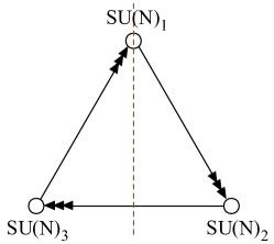
Figure 10: The quiver for $\mathbb{C}^{3}/\mathbb{Z}_{3}$, with the involution of interest indicated by the dashed line.

Applying the rules of §A.1, we search for orientifolds of this configuration. Inspecting the quiver, one can easily check that rule I implies that the involution must fix one node and exchange the other two. As the quiver has a $\mathbb{Z}_{3}$ symmetry, we take the fixed node to be node $1$ WLOG. The action of the involution on the chiral superfields is then:

$$X_{12}^{i}\to\Lambda^{i}_{\,j}\,\mathcal{I}_{1}(X_{31}^{j})^{T}\delta_{32}^{*}\,,\quad X_{23}^{i}\to\Sigma^{i}_{\,j}\,\delta_{23}(X_{23}^{j})^{T}\delta_{23}^{*}\,,\quad X_{31}^{i}\to(\Lambda^{i}_{\,j})^{{\dagger}}\,\delta_{32}(X_{12}^{j})^{T}\mathcal{I}_{1}^{*}\,,$$ (618)

where $\Lambda$ and $\Sigma$ are unitary matrices, $\delta_{23}=\delta_{32}^{T}=\text{1}$ breaks $SU(N)_{2}\times SU(N)_{3}\to SU(N)$, and $\mathcal{I}_{1}=\text{1}$ or $\Omega$, depending on whether we choose an $SO$ or $U\!Sp$ projection for the fixed node, respectively. Moreover, since the involution squares to the identity, $\Sigma^{2}=\text{1}$, so that $\Sigma$ is both unitary and Hermitian.

We compute the orientifold image of the superpotential:

$$W\to W^{\prime} = \epsilon_{ijk}\,\Lambda^{i}_{\,i^{\prime}}\Sigma^{j}_{\,j^{\prime}}(\Lambda^{k}_{\,k^{\prime}})^{{\dagger}}\,\mathrm{Tr\,}\mathcal{I}_{1}(X_{31}^{i^{\prime}})^{T}\delta_{32}^{*}\,\delta_{23}(X_{23}^{j^{\prime}})^{T}\delta_{23}^{*}\,\delta_{32}(X_{12}^{k^{\prime}})^{T}\mathcal{I}_{1}^{*}$$ (619)

$$= (\pm_{\rm Sp})\,\epsilon_{ijk}\,\Lambda^{i}_{\,i^{\prime}}\Sigma^{j}_{\,j^{\prime}}(\Lambda^{k}_{\,k^{\prime}})^{{\dagger}}\,\mathrm{Tr\,}X_{12}^{k^{\prime}}X_{23}^{j^{\prime}}X_{31}^{i^{\prime}}\,.$$

Therefore, invariance of the superpotential requires:

$$\epsilon_{ijk}\,\Lambda^{i}_{\,i^{\prime}}\Sigma^{j}_{\,j^{\prime}}(\Lambda^{k}_{\,k^{\prime}})^{{\dagger}}=-(\pm_{\rm Sp})\,\epsilon_{i^{\prime}j^{\prime}k^{\prime}}\,.$$ (620)

In fact, this is only possible if $\Lambda=e^{i\theta}\Sigma$, where the phase factor can be removed by rotating $X_{12}^{i}\to e^{i\theta/2}X_{12}^{i}$ and $X_{31}^{i}\to e^{-i\theta/2}X_{31}^{i}$ (leaving the superpotential invariant). Thus, we take $\Lambda=\Sigma$, where the invariance of the superpotential requires

$$\det\Sigma=-(\pm_{\rm Sp})\,.$$ (621)

After an $SU(3)$ transformation, we obtain $\Sigma=\operatorname{diag}(\pm_{1},\pm_{2},\pm_{3})$, and the requirement that the superpotential be invariant takes the form of a sign rule:

$$(\pm_{1})(\pm_{2})(\pm_{3})(\pm_{\rm Sp})=-1\,.$$ (622)

Thus, for an $SO$ projection, there are two possible involutions $\Sigma=\operatorname{diag}(-,-,-)$ and $\Sigma=\operatorname{diag}(-,+,+)$ up to an $SU(3)$ transformation. The spectrum of the latter theory turns out to be anomalous for any choice of gauge group ranks, so we will focus on the first possibility. Similarly, for an $U\!Sp$ projection, $\Sigma=\operatorname{diag}(+,+,+)$ and $\Sigma=\operatorname{diag}(-,-,+)$ are possible, again up to an $SU(3)$ transformation, with the latter being anomalous for any choice of ranks.

The anomalous orientifolds correspond to noncompact O7 planes, whereas the remaining possibilities correspond to compact O7 planes Franco:2010jv . We verify this by computing the geometric involution. Consider mesons of the form:

$$Z^{ijk}\equiv\mathrm{Tr\,}X_{12}^{i}X_{23}^{j}X_{31}^{k}\,.$$ (623)

Upon imposing the F-term conditions, we find that $Z^{ijk}$ is totally symmetric in its indices. Applying the involution (618), we obtain:

$$Z^{ijk}\to(\pm_{\rm Sp})\,\Sigma^{i}_{\,i^{\prime}}\Sigma^{j}_{\,j^{\prime}}\Sigma^{j}_{\,j^{\prime}}Z^{i^{\prime}j^{\prime}k^{\prime}}=[(\pm_{\rm Sp})\Sigma^{i}_{\,i^{\prime}}]\,[(\pm_{\rm Sp})\Sigma^{j}_{\,j^{\prime}}]\,[(\pm_{\rm Sp})\Sigma^{k}_{\,k^{\prime}}]\,Z^{i^{\prime}j^{\prime}k^{\prime}}\,,$$ (624)

where the sign $\pm_{\rm Sp}$ comes from the $\Omega^{2}=-1$ which appears in the trace for $U\!Sp$ projections. The mesons $Z^{ijk}$ correspond to the coordinates $z^{i}z^{j}z^{k}$ of $\mathbb{C}^{3}/\mathbb{Z}_{3}$; thus, we read off the geometric involution

$$z^{i}\to(\pm_{\rm Sp})\,\Sigma^{i}_{j}z^{j}\,.$$ (625)

From this, it is easy to check that the anomaly-free orientifolds, $(-,-,-)$ and $(+,+,+)$ for $SO$ and $U\!Sp$ respectively, correspond to compact O7 planes, with the involution $z^{i}\to-z^{i}$, whereas the anomalous orientifolds, $(-,+,+)$ and $(+,-,-)$ for $SO$ and $U\!Sp$ respectively, correspond to noncompact O7 planes, with the involution $z^{1}\to-z^{1}$, $z^{2}\to z^{2}$, $z^{3}\to z^{3}$.

To derive the superpotential of the orientifold theory, we replace:

$$X_{12}^{i} \to \Sigma^{i}_{j}\,A^{j}\,,$$

$$X_{23}^{i} \to \Sigma^{i}_{k}\,B^{j}\,\delta_{23}^{*}\,,$$

$$X_{31}^{i} \to \delta_{32}\,(A^{j})^{T}\mathcal{I}_{1}^{*}\,,$$ (626)

where invariance under the involution requires that:

$$B^{i}=\Sigma^{i}_{\,j}\,(B^{j})^{T}\,,$$ (627)

so that for $\Sigma=\operatorname{diag}(\pm_{1},\pm_{2},\pm_{2})$, $B^{i}$ is symmetric (antisymmetric) when $\pm_{i}$ is positive (negative). Applying these replacements to the superpotential, we obtain:

$$W=\frac{1}{2}(\det\Sigma)\,\epsilon_{ijk}\Sigma^{k}_{\,l}\,\mathrm{Tr\,}A^{i}B^{j}(A^{l})^{T}\,,$$ (628)

where for $U\!Sp$ projections the use of $\Omega$ in the trace is implicit. Since $\mathrm{Tr\,}M=\mathrm{Tr\,}M^{T}$, this can also be written as:

$$W=(\pm_{\rm Sp})\frac{1}{2}(\det\Sigma)\,\epsilon_{ijk}\Sigma^{k}_{\,l}\,\Sigma^{j}_{m}\,\mathrm{Tr\,}A^{l}B^{m}(A^{i})^{T}=-(\pm_{\rm Sp})(\det\Sigma)\,W\,.$$ (629)

Thus, as before, the sign rule (621) is necessary to ensure that the superpotential of the orientifold theory does not vanish.

For the cases $\Sigma=\operatorname{diag}(-,-,-)$ and $\Sigma=\operatorname{diag}(+,+,+)$ for $SO$ and $U\!Sp$ projections, respectively, the superpotential simplifies:

$$W=\frac{1}{2}\,\epsilon_{ijk}A^{i}A^{j}B^{k}\,,$$ (630)

where we leave the contractions of gauge indices implicit. The resulting theories have the same $SU(3)\times U(1)_{R}$ flavor symmetries as the parent quiver theory, and are discussed more thoroughly in §3.

A.3 General Quiverfolds

In the simple examples discussed above, we applied the rules of §A.1 in a straightforward (if tedious) fashion to rederive known results. We now discuss some general features of this program applied to arbitrary quiver gauge theories. Specifically, we show how to derive the gauge group and spectrum of the orientifold theory graphically using the quiver diagram, and define a suitable generalization of the quiver to represent these data.

For the purposes of this discussion, we mainly ignore the superpotential, though we emphasize that rule II is generally very restrictive, and not all involutions of the quiver will leave the superpotential invariant. An explicit computation to check that $W$ is invariant under the involution can be tedious, and for toric singularities the problem is well suited to brane tiling methods, as originally formulated in Franco:2007ii and reviewed in transitions3 .

Rule I implies that the quiver of the parent theory possesses a $\mathbb{Z}_{2}$ charge conjugation (arrow reversing) symmetry representing the involution in question. We embed the quiver in $\mathbb{R}^{2}$ such that this symmetry is manifest as a reflection through a fixed line, as in figure 9. In the resulting figure, fixed nodes must lie along the fixed line, and fixed edges will intersect it perpendicularly, whereas any unfixed edge which crosses the fixed line must intersect another edge (its image) at the point of crossing.

To obtain the gauge group and spectrum of the orientifold theory we cut the plane in two along the fixed line, discarding one half of it and labeling each node and perpendicular (fixed) edge along the boundary with a sign. The resulting diagram on the half-plane, which we call a “quiverfold”, specifies the gauge group and spectrum of the orientifold theory as follows: each node away from the boundary (“whole” node) corresponds to an $SU$ gauge group, whereas each $+$ ($-$) node along the boundary (“half” node) corresponds to an $SO$ ($U\!Sp$) gauge group. Each arrow away from the boundary (“uncrossed” (whole) edge) corresponds to bifundamental $(\leavevmode\hbox{\vtop{\offinterlineskip\openup-0.4pt\halign{&\startbox@YT{\defarg@YT}{}#\endbox@YT\cr\framebox{\vbox to5.0pt{\vss\hbox to5.0pt{\hss$$\hss}\vss}}\cr}}\kern 5.0pt},\bar{\leavevmode\hbox{\vtop{\offinterlineskip\openup-0.4pt\halign{&\startbox@YT{\defarg@YT}{}#\endbox@YT\cr\framebox{\vbox to5.0pt{\vss\hbox to5.0pt{\hss$$\hss}\vss}}\cr}}\kern 5.0pt}})$ matter in the usual way, while each arrow intersecting the boundary obliquely is joined to its image arrow to form an edge (“crossed” (whole) edge) with opposite orientations associated to each end, and corresponding to $(\leavevmode\hbox{\vtop{\offinterlineskip\openup-0.4pt\halign{&\startbox@YT{\defarg@YT}{}#\endbox@YT\cr\framebox{\vbox to5.0pt{\vss\hbox to5.0pt{\hss$$\hss}\vss}}\cr}}\kern 5.0pt},\leavevmode\hbox{\vtop{\offinterlineskip\openup-0.4pt\halign{&\startbox@YT{\defarg@YT}{}#\endbox@YT\cr\framebox{\vbox to5.0pt{\vss\hbox to5.0pt{\hss$$\hss}\vss}}\cr}}\kern 5.0pt})$ or $(\bar{\leavevmode\hbox{\vtop{\offinterlineskip\openup-0.4pt\halign{&\startbox@YT{\defarg@YT}{}#\endbox@YT\cr\framebox{\vbox to5.0pt{\vss\hbox to5.0pt{\hss$$\hss}\vss}}\cr}}\kern 5.0pt}},\bar{\leavevmode\hbox{\vtop{\offinterlineskip\openup-0.4pt\halign{&\startbox@YT{\defarg@YT}{}#\endbox@YT\cr\framebox{\vbox to5.0pt{\vss\hbox to5.0pt{\hss$$\hss}\vss}}\cr}}\kern 5.0pt}})$, depending on the orientation of the arrows. Finally, each $+$ ($-$) edge ending perpendicularly on the boundary (“half” edge) corresponds to symmetric (antisymmetric) matter.

An example quiverfold is shown in figure 11(a). As shown in figure 11(b – c), the quiverfold can be drawn without the boundary line by using appropriate symbols to denote the fixed elements and crossed edges. From this perspective, a quiverfold is just an “enhanced” quiver, with a few additional representations and gauge groups allowed. Just as the worldvolume gauge theory on intersecting D-branes can always be represented by a quiver gauge theory, orientifolds of these configurations can always be represented by a quiverfold (to the extent that rule I holds), which is then a very useful tool for concisely stating the gauge group and spectrum.

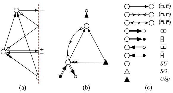
Figure 11: (a) An example of a quiverfold. The parent quiver is shown in figure 9. (b) The quiverfold can be redrawn without the fixed line using appropriate symbols, defined in (c).

Note that some apparently different quiverfolds are isomorphic. In particular, any whole node of the quiverfold can be charge conjugated, yielding a new, equivalent quiverfold with different crossed and uncrossed edges; this corresponds to swapping the positions of a node and its image in the original $\mathbb{Z}_{2}$ symmetric embedding of the quiver. In a strict quiver, there is no analogous operation: since crossed edges are not allowed, charge conjugation can only be applied to the quiver as a whole. Furthermore, not every edge of a quiverfold is directed at both ends, since arrows entering and exiting half nodes are equivalent. Thus, edges connecting a half node to a whole node have a single direction (they cannot be crossed), whereas edges connecting two half-nodes are undirected. Taking into account these isomorphisms, it is straightforward to show that different $\mathbb{R}^{2}$ embeddings of the same involution (with the same choice of fixed-element signs) lead to the same quiverfold. Moreover, given a quiverfold, it is possible to uniquely reconstruct the parent quiver and involution by embedding the quiverfold on the half-plane with fixed elements on the boundary, as above.

It should be emphasized that just as a quiver is a direct pictorial representation of a certain class of gauge theories (quiver gauge theories), a quiverfold is also a direct pictorial representation of a certain (somewhat broader) class of gauge theories, which we call quiverfold gauge theories. Just as gauge invariant (mesonic) operators are directed loops in the quiver diagram, gauge invariant (mesonic) operators are loops in the quiverfold, subject to the requirement that the loop enter and exit each whole node on oppositely directed edges. However, in some cases the mesonic operator corresponding to such a loop vanishes due to symmetry (e.g. it takes the form $\mathrm{Tr\,}M$ where $M$ is antisymmetric).

While quiverfolds are useful for computing and representing the gauge group and spectrum of a given orientifold, the set of involutions consistent with rule I is usually a superset of those involutions consistent with both rules I and II: as we saw in §A.2, the invariance of the superpotential imposes important constraints, such as the sign rules (607), (622) and (in the latter case) the alignment of the flavor rotations $\Lambda^{i}_{\,j}$ and $\Sigma^{i}_{\,j}$.

It is possible to reformulate rule II graphically by describing the parent gauge theory and the involution in terms of a brane tiling, rather than a quiver diagram. We refer the interested reader to Franco:2007ii for further details and references. As shown in transitions3 , this approach is equivalent to the one outlined here. Regardless of the method used to apply these rules, quiverfold diagrams provide an intuitive and precise representation of the gauge group and spectrum of the orientifold gauge theory, much like quiver diagrams for D-brane gauge theories.

Appendix B Negative rank duality

In this appendix we review a fact about continuing $SU(N)$, $SO(N)$ and $U\!Sp(N)$ groups to negative rank that turns out to be very useful in the anomaly matching discussion in the main text. We refer the reader to chapter 13 in Cvitanovic:2008zz for more details and further references. As we explain below, this continuation relates for example an $SU(-N)$ gauge theory to an $\widetilde{SU(N)}$ gauge theory and is often referred to as negative rank duality although the two related theories are generically not dual in the physical sense. In particular the two related gauge theories have generically different anomalies.

For an $SU(N)$ gauge theory with matter in certain representation we can exchange symmetrization and antisymmetrization (i.e. reflect the Young tableau across the diagonal) and at the same time replace $N$ with $-N$. This leads to a new gauge theory we denote $\widetilde{SU(N)}$. As was first noticed by King , for $SO(N)$ and $U\!Sp(N)$ theories we can likewise obtain a negative rank dual theory by exchanging symmetrization and antisymmetrization and replacing the $SO(N)$ symmetric bilinear invariant $\delta_{ab}$ by the $U\!Sp(N)$ antisymmetric bilinear invariant $\Omega_{ab}$ and replacing $N$ by $-N$: $SO(-N)\cong\widetilde{U\!Sp(N)}$, $U\!Sp(-N)\cong\widetilde{SO(N)}$.

In Cvitanovic:2008zz it is proven that under these dualities any scalar quantity becomes the dual scalar quantity up to potentially an overall sign. In particular, if we have a matter field transforming in the representation $r$ which has a Young tableau with $p$ boxes and $\tilde{r}$ denotes the transposed tableau obtained by a flip across the diagonal, then the dimensions of the corresponding representations are related by

$$d_{N}(r)=(-1)^{p}d_{-N}(\tilde{r})\,.$$ (637)

Thanks to the theorems of Cvitanovic:2008zz that we mentioned above, the proof is simple since we only need to determine the overall sign $(-1)^{p}$: Any representation with $p$ boxes in the Young tableau has a leading $N$ scaling that is given by $N^{p}$ so that the overall sign under changing $N\rightarrow-N$ is $(-1)^{p}$, which gives the stated result.

Below we study the anomalies of negative rank dual theories of a generic gauge theory (see Maru:1996fq for related results). For that we need the transformation properties of the Dynkin index $T(r)$ and anomaly coefficient $A(r)$ under the negative rank duality. These are again determined by the leading $N$ scaling. Contrary to the dimension the Dynkin index and anomaly coefficient of the fundamental representation are independent of $N$. However, similarly to the dimension any extra box in the Young tableau leads to an extra factor of $N$ so that one finds

$$T_{N}(r)=(-1)^{p-1}T_{-N}(\tilde{r})\,,\qquad A_{N}(r)=(-1)^{p-1}A_{-N}(\tilde{r})\,.$$ (638)

To prove this, we can again derive the leading $N$ scaling by calculating the Dynkin index and anomaly coefficient for the tensor product of $p$ fundamental representations. The Dynkin index $T(r)$ is defined by $(T^{a}_{r})^{m}_{n}(T^{b}_{r})^{n}_{m}=T(r)\delta^{ab}$, where the $T^{a}_{r}$ are the generators for the representation $r$. Taking the tensor product with another fundamental representation introduces a factor of $N$ in $T(r)$ and taking the tensor product of a fundamental with $(p-1)$ fundamental representation leads to the above result. Explicitly, for $SU(N)$ we can choose one of the generators in the fundamental representation to be $T^{1}_{\leavevmode\hbox{\vtop{\offinterlineskip\openup-0.4pt\halign{&\startbox@YT{\defarg@YT}{}#\endbox@YT\cr\framebox{\vbox to3.5pt{\vss\hbox to3.5pt{\hss$$\hss}\vss}}\cr}}\kern 3.5pt}}=\tfrac{1}{\sqrt{2((N-1)^{2}+N-1)}}\text{diag}(1,1,\ldots,1,-(N-1))$, which leads to $T(\leavevmode\hbox{\vtop{\offinterlineskip\openup-0.4pt\halign{&\startbox@YT{\defarg@YT}{}#\endbox@YT\cr\framebox{\vbox to5.0pt{\vss\hbox to5.0pt{\hss$$\hss}\vss}}\cr}}\kern 5.0pt})=\tfrac{1}{2}$. The leading $N$ scaling for any representation with $p$ boxes is the same as the leading $N$ scaling for the tensor product of $p$ fundamentals. Taking $p-1$-times the tensor product of the above generator with $\text{1}_{N}$ we obtain a generator for the representation that is given by the tensor product of $p$ fundamentals and we find the leading $N$ term $T(r)\propto N^{p-1}$, which is true for all irreducible representation of $SU(N)$ with $p$ boxes. Similarly one can explicitly work out the scaling for $SO(N)$ and $U\!Sp(N)$. For the anomaly coefficient of $SU(N)$, we us the following result from Banks:1976yg : $A(r_{1}\otimes r_{2})=d(r_{1})A(r_{2})+d(r_{2})A(r_{1})$. Together with the fact that $A(\leavevmode\hbox{\vtop{\offinterlineskip\openup-0.4pt\halign{&\startbox@YT{\defarg@YT}{}#\endbox@YT\cr\framebox{\vbox to5.0pt{\vss\hbox to5.0pt{\hss$$\hss}\vss}}\cr}}\kern 5.0pt})$ is $N$ independent this leads to the leading $N$ scaling $A(r)\propto N^{p-1}$ which completes the proof.

We now show that for any gauge theory the negative rank dual is free of gauge anomalies if all chiral matter representations have dimensions that are even under the negative rank dual i.e. whenever for every chiral field the number of all boxes in the Young tableaux of all gauge theories we are dualizing is even. Furthermore, the global anomalies of the two theories are related by replacing the rank of each gauge group factor we are dualizing with its negative and adding an overall minus sign whenever the global anomaly involves a non-abelian gauge group that is also being dualized.

We take the combined gauge and global symmetry group to be $G=U(1)_{1}\times\ldots\times U(1)_{m}\times G_{1}\times\ldots\times G_{n}$, where $G_{a}$ are $SU$, $SO$ or $U\!Sp$ groups. We denote the chiral matters fields by $\chi$, the corresponding $U(1)_{i}$ charges by $q_{i}^{\chi}$ and the matter dimension by $d(\chi)=\prod_{a=1}^{n}d(r_{\chi}^{G_{a}})$ where $r_{\chi}^{G_{a}}$ denotes the representation of $\chi$ under the group $G_{a}$. The $U(1)^{3}$ and $U(1)$ anomalies are given by

$$U(1)_{i}\,U(1)_{j}\,U(1)_{k} = \sum_{\chi}d(\chi)q_{i}^{\chi}q_{j}^{\chi}q_{k}^{\chi}\,,$$ (642)

$$U(1)_{i} = \sum_{\chi}d(\chi)q_{i}^{\chi}\,,$$ (643)

where the sums are over all chiral superfields $\chi$. Whenever all chiral matter fields satisfy $d(\chi)=d(\tilde{\chi})$, then the above anomalies are unchanged after dualizing any of the $G_{a}$. The $G^{2}\,U(1)$ and $G^{3}$ anomalies are

$$G_{a}^{2}\,U(1)_{i} = \sum_{\chi}\frac{d(\chi)}{d(r_{\chi}^{G_{a}})}T(r_{\chi}^{G_{a}}))q_{i}^{\chi}\,,$$ (644)

$$G_{a}^{3} = \sum_{\chi}\frac{d(\chi)}{d(r_{\chi}^{G_{a}})A(r_{\chi}(G_{a}))}\,.$$ (645)

If $G_{a}$ does not undergo a negative rank transition then the above anomalies are unchanged. In the case that $G_{a}$ undergoes a negative rank duality we use the fact that $T(r)/d(r)=-T(\tilde{r})/d(\tilde{r})$ and $A(r)/d(r)=-A(\tilde{r})/d(\tilde{r})$ to find that both of the anomalies above pick up an extra minus sign. In particular this means that all the gauge and mixed anomalies that do not involve the R-symmetry still vanish after the negative rank transition. In our examples the global non-abelian gauge groups will not undergo a negative rank transition so that none of the global anomalies pick up an extra minus sign. They are simply given by replacing the ranks of all the gauge groups that undergo the negative rank duality with their negative ranks.

Next we calculate the anomalies that involve the R-symmetry

$$U(1)_{R}^{3} = \sum_{\chi}d(\chi)(q_{R}^{\chi}-1)^{3}+d(G_{gauge})\,,$$ (646)

$$U(1)_{i}\,U(1)_{R}^{2} = \sum_{\chi}d(\chi)q_{i}(q_{R}^{\chi}-1)^{2}\,,$$ (647)

$$U(1)_{i}\,U(1)_{j}\,U(1)_{R} = \sum_{\chi}d(\chi)q_{i}q_{j}(q_{R}^{\chi}-1)\,,$$ (648)

$$U(1)_{R} = \sum_{\chi}d(\chi)(q_{R}^{\chi}-1)+d(G_{gauge})\,,$$ (649)

$$G_{a}^{2}\,U(1)_{R} = \sum_{\chi}\frac{d(\chi)}{d(r_{\chi}^{G_{a}})}T(r_{\chi}^{G_{a}})(q_{R}^{\chi}-1)+T(\text{Adj}_{G_{a}})\,.$$ (650)

Above $d(G_{gauge})$ denotes the dimension of the entire gauge group (excluding the global symmetry group) and $T(\text{Adj}_{G_{a}})$ denotes the Dynkin index of the adjoint of $G_{a}$, if $G_{a}$ is part of the gauge group. If $G_{a}$ is part of the global symmetry group, then there are no gauginos that contribute and we have to set $T(\text{Adj}_{G_{a}})=0$. For the $SU$, $SO$ and $U\!Sp$ groups the group dimension has always even parity under the negative rank transition. Thus $d(G_{gauge})$ is even and as mentioned above $T(\text{Adj}_{G_{a}})$ is odd, if $G_{a}$ undergoes the negative rank transition since $p=2$. This means that only the last of the anomalies above picks up an overall minus sign if $G_{a}$ undergoes the negative rank transition. We thus conclude that all gauge and mixed anomalies vanish after the transition. In the case where none of the global non-abelian symmetry groups undergo a negative rank transition we can furthermore conclude that all anomalies of the negative rank dual theory are obtained by replacing the ranks of all gauge group factors that undergo the transition with their negative.

A simple example of two negative rank dual theories has already appeared above in §3. Both theories are related by taking the negative rank dual of both gauge group factors. The $SO(N-4)\times SU(N)$ extrapolated to negative $N$ is $SO(-(N+4))\times SU(-N)$ which dualizes to $U\!Sp(N+4)\times SU(N)$. We also have to flip the Young tableaux so that the antisymmetric representation of $SU(-N)$ becomes the symmetric representation of $SU(N)$. The usefulness of this duality is that we did not have to calculate the anomalies in §3.1 for both theories, since they are related by changing the sign of $N$. Since the anomalies depend on $N(N-3)$ which becomes $N(N+3)$ we see that the two negative rank dual theories are not dual in the physical sense since they have different anomalies. In this particular case the negative rank dual is however dual to the original theory after shifting the ranks of the gauge groups.

Appendix C Exactly dimensionless couplings

Under certain assumptions, a sufficient condition for a holomorphic coupling to be constant along the RG flow is that it be neutral under all possible flavor symmetries, in particular those which are spurious and/or anomalous.

We focus first on the case where there are no nonabelian flavor symmetries. Due to various nonrenormalization theorems (see e.g. Terning:2006bq ), holomorphic couplings are not perturbatively renormalized apart from the one-loop running of holomorphic gauge couplings. Thus, in the absence of nonperturbative renormalization of these couplings, holomorphic couplings are independent of scale, provided we replace the scale-dependent holomorphic gauge couplings $\tau(\mu)$ with the holomorphic dynamical scale $\Lambda\equiv\mu e^{2\pi i\tau(\mu)/b}$, where $b=3T(\text{Adj})-T({\rm mat})$ is the one-loop beta function coefficient (if $b=0$ then $\Lambda$ is ill-defined but $\tau$ itself is independent of scale).

However, non-holomorphic couplings are not likewise protected against renormalization, and in particular chiral superfields are subject to wave-function renormalization through corrections to the Kähler potential. Rescaling the chiral superfields to restore canonical normalization leads to rescaling anomalies which alter the values of the holomorphic couplings, leading to a nontrivial running for their physical (canonically normalized) counterparts. In particular, the rescaling may be realized as a complexification of a $U(1)$ symmetry under which the chiral superfield in question is charged, whereas the corresponding $U(1)$ may be spurious and/or anomalous, leading to a rescaling of the corresponding spurions (superpotential couplings) and/or the holomorphic dynamical scale(s) of the gauge theory Terning:2006bq . However, if a certain holomorphic combination of couplings is neutral under all of these $U(1)$’s, then it is unaffected by the rescaling, and therefore the corresponding physical coupling is scale independent (has vanishing anomalous dimension). Such a coupling is exactly dimensionless if and only if it is classically dimensionless. This is readily shown to be equivalent to the requirement that the coupling is neutral under the $U(1)_{R}$ under which all chiral superfields carry charge $+2/3$.

Thus, a holomorphic coupling corresponds to an exactly dimensionless physical (canonically normalized) coupling if it is neutral under all possible $U(1)$ and $U(1)_{R}$ symmetries (since an arbitrary $U(1)_{R}$ is a linear combination of an arbitrary $U(1)$ with the “canonical” $U(1)_{R}$ considered above), assuming that none of the constituent couplings are nonperturbatively renormalized. While the converse need not be true, the existence of an exactly marginal holomorphic coupling which violates these conditions imposes a nontrivial relation on the anomalous dimensions along the flow. Since anomalous dimensions typically cannot be computed exactly away from an infrared fixed point, computable examples without extended supersymmetry must satisfy these conditions.

If the gauge group is semi-simple, a straightforward counting argument gives the number $N_{0}$ of exactly dimensionless couplings of this type for a model with $N_{G}$ (simple) gauge groups, $N_{W}$ superpotential terms (each with a corresponding coupling), $N_{\chi}$ chiral superfields, and $N_{U(1)}$ linearly independent “good” $U(1)$ or $U(1)_{R}$ symmetries (not broken by gauge anomalies or by the superpotential):

$$N_{0}=N_{U(1)}+N_{G}+N_{W}-(N_{\chi}+1)\,.$$ (651)

The argument is as follows: there are $N_{\chi}+1$ linearly independent spurious and/or anomalous $U(1)$ or $U(1)_{R}$ symmetries in general, whereas the “good” $U(1)$’s are those under which the $N_{G}+N_{W}$ holomorphic couplings are neutral, and can be represented by vectors of length $N_{\chi}+1$ which are annihilated by the $(N_{G}+N_{W})\times(N_{\chi}+1)$ matrix of $U(1)$ charges of the holomorphic couplings acting on the left. The rank of this matrix is therefore $N_{\chi}+1-N_{U(1)}$. By contrast, an exactly dimensionless coupling is a product of holomorphic couplings which is neutral under all the $U(1)$’s, and can be represented by a vector of length $N_{G}+N_{W}$ which is annihilated by the same matrix acting on the right. Since row rank and column rank are equal, the number of linearly independent vectors of this type is $N_{G}+N_{W}-(N_{\chi}+1-N_{U(1)})$, reproducing the above formula.

These arguments must be modified to include any (potentially spurious) non-abelian flavor symmetries, since chiral multiplets with the same gauge quantum numbers are subject to kinetic mixing (unless forbidden by the global symmetries). In particular, the candidate combination of couplings must also be neutral under these non-abelian symmetries in addition to the $U(1)$ and $U(1)_{R}$ symmetries as a sufficient condition for exact marginality.

Let $G_{F}$ denote the semisimple component of the spurious flavor symmetries. Since only $G_{F}$-singlet combinations of couplings can appear in our candidate exactly dimensionless couplings and the holomorphic gauge couplings are all neutral under $G_{F}$, we need only consider $G_{F}$-invariant combinations of superpotential couplings. We can then treat $G_{F}$ as if it were gauged (without the corresponding gauge coupling). Thus, the above counting argument still holds, where now $N_{\chi}$ counts the number of irreducible $G_{F}$ multiplets, $N_{W}$ the number of independent $G_{F}$ invariant combinations of superpotential couplings, and $N_{U(1)}$ counts the number of “good” $U(1)$ or $U(1)_{R}$ symmetries which commute with $G_{F}$.

C.1 On nonperturbative effects

So far we have ignored the possibility that the holomorphic couplings run due to nonperturbative effects. While it is not possible to exclude this in general, such effects are also constrained by nonrenormalization theorems, and are known to be absent in some simple cases, such as pure $\mathcal{N}=1$ super-Yang-Mills ArkaniHamed:1997mj .

In particular, for the gauge theories studied in this paper, we are interested in whether the string coupling $\tau_{\rm 10d}$ (40) — which is not perturbatively renormalized by the above criteria — can run nonperturbatively. A spurion analysis reveals that the exact (Wilsonian) beta function must take the form:

$$\mu\frac{d}{d\mu}\tau_{\rm 10d}=f(\tau_{\rm 10d})$$ (652)

where $f(\tau_{\rm 10d})$ is a holomorphic function satisfying $f(+i\infty)=0$ due to the lack of perturbative running, and $f$ cannot depend on any other holomorphic couplings due to constraints imposed by the spurious and/or anomalous $U(1)$ symmetries.

We first consider the $SO$ theory for even $N$, where $SL(2,\mathbb{Z})$ covariance requires that

$$f\left(\frac{a\tau+b}{c\tau+d}\right)=(c\tau+d)^{-2}f(\tau)$$ (653)

Hence $f(\tau)$ is a modular form of weight $-2$. However, no such holomorphic modular form exists. Instead, such a modular form is necessarily meromorphic, with poles in the upper half plane $\mathbb{H}$ where the beta function blows up at finite coupling. Such poles signal a breakdown of the Wilsonian description, and are likely inconsistent. Analogous statements hold for odd $N$ (and for the $U\!Sp$ theory) where $SL(2,\mathbb{Z})$ becomes $\Gamma_{0}(2)$ and $f$ is a level-two modular form. Hence, we conclude that $f(\tau)=0$, and $\tau_{\rm 10d}$ is not renormalized in either theory.

Appendix D Coulomb branch computation of the string coupling

In this appendix, we provide a derivation of (40) for completeness. A similar computation can be done for gauge theories arising from more complicated geometries.

To establish this result, we consider the $SO(N-4+2k)\times SU(N+2k)$ theory and switch on a mesonic vev, removing $k$ D3 branes from the orientifold plane and breaking the gauge group down to $SO(N-4)\times SU(N)\times U(k)$, where the last factor corresponds to the $\mathcal{N}=4$ gauge theory on the $k$ D3 branes. The holomorphic gauge coupling of $U(k)$ is therefore equal to the ten-dimensional axio-dilaton, and by performing scale matching at each step of the computation, we can relate it to the couplings of the $SO(N-4)\times SU(N)$ theory, giving (40).

We now sketch the details of this argument. For simplicity, we routinely drop numerical factors throughout the computation, only keeping track of the dependence on the couplings. We aim to turn on a vev which breaks

$$SO(N-4+2k)\times SU(N+2k)\longrightarrow SO(N-4)\times SU(N)\times U(k)\,,$$ (654)

corresponding to removing D3 branes from the orientifold plane. In particular, a suitable $B$ vev will break $SU(N+2k)\rightarrow SU(N)\times U\!Sp(2k)$, whereas an $A$ vev will then break $SO(N-4+2k)\times U\!Sp(2k)\rightarrow SO(N-4)\times U(k)$, since Higgsing a bifundamental breaks $SO(2k)\times U\!Sp(2k)\rightarrow U(k)$. For a suitable normalization of the $U(1)$ component, we have the decomposition

$$\leavevmode\hbox{\vtop{\offinterlineskip\openup-0.4pt\halign{&\startbox@YT{\defarg@YT}{}#\endbox@YT\cr\framebox{\vbox to5.0pt{\vss\hbox to5.0pt{\hss$$\hss}\vss}}\cr}}\kern 5.0pt}\rightarrow\leavevmode\hbox{\vtop{\offinterlineskip\openup-0.4pt\halign{&\startbox@YT{\defarg@YT}{}#\endbox@YT\cr\framebox{\vbox to5.0pt{\vss\hbox to5.0pt{\hss$$\hss}\vss}}\cr}}\kern 5.0pt}_{\,+1}\oplus\overline{\leavevmode\hbox{\vtop{\offinterlineskip\openup-0.4pt\halign{&\startbox@YT{\defarg@YT}{}#\endbox@YT\cr\framebox{\vbox to5.0pt{\vss\hbox to5.0pt{\hss$$\hss}\vss}}\cr}}\kern 5.0pt}}_{\,-1}\,,$$ (658)

for both $SO(2k)\rightarrow U(k)$ and $U\!Sp(2k)\rightarrow U(k)$. Thus, decomposing $A^{i}$ and $B^{i}$ into irreps of $SO(N-4)\times SU(N)\times U(k)$, we find

for each of the three $SU(3)$ “flavors” of each field, where $\text{Adj}_{0}$ denotes the reducible $U(k)$ adjoint representation of dimension $k^{2}$, containing both singlet and trace-free irreps.

We choose to turn on a vev for the singlet components of $A^{3}$ and $B^{3}$ only, which implies that only components of these fields can be Higgsed. We have broken $3(2N-3)k+5k^{2}$ generators, therefore

$$\frac{3(N+2k)(N+2k-3)}{2}-3(2N-3)k-5k^{2}=\frac{3N(N-3)}{2}+k^{2}$$ (685)

chiral superfields remain unHiggsed. The only way to get the correct scaling with $N$ and $k$ is if the unHiggsed fields are

$$(\leavevmode\hbox{\vtop{\offinterlineskip\openup-0.4pt\halign{&\startbox@YT{\defarg@YT}{}#\endbox@YT\cr\framebox{\vbox to5.0pt{\vss\hbox to5.0pt{\hss$$\hss}\vss}}\cr}}\kern 5.0pt},\overline{\leavevmode\hbox{\vtop{\offinterlineskip\openup-0.4pt\halign{&\startbox@YT{\defarg@YT}{}#\endbox@YT\cr\framebox{\vbox to5.0pt{\vss\hbox to5.0pt{\hss$$\hss}\vss}}\cr}}\kern 5.0pt}},1)\oplus\left(1,\leavevmode\hbox{\vtop{\offinterlineskip\openup-0.4pt\halign{&\startbox@YT{\defarg@YT}{}#\endbox@YT\cr\framebox{\vbox to5.0pt{\vss\hbox to5.0pt{\hss$$\hss}\vss}}\cr\framebox{\vbox to5.0pt{\vss\hbox to5.0pt{\hss$$\hss}\vss}}\cr}}\kern 5.0pt},1\right)\oplus(1,1,\text{Adj}_{0})\,,$$ (690)

coming from $A^{3}$, $B^{3}$, and a linear combination of the two, respectively. Thus, the matter content just below the Higgsing scale $v$ is precisely:

$$\begin{array}[]{c|ccc|ccc}\mathrm{origin}&SO(N-4)&SU(N)&U(k)&SU(2)&U(1)_{R}^{\prime}&\#\\ \hline\cr A&\leavevmode\hbox{\vtop{\offinterlineskip\openup-0.4pt\halign{&\startbox@YT{\defarg@YT}{}#\endbox@YT\cr\framebox{\vbox to5.0pt{\vss\hbox to5.0pt{\hss$$\hss}\vss}}\cr}}\kern 5.0pt}&\overline{}\leavevmode\hbox{\vtop{\offinterlineskip\openup-0.4pt\halign{&\startbox@YT{\defarg@YT}{}#\endbox@YT\cr\framebox{\vbox to5.0pt{\vss\hbox to5.0pt{\hss$$\hss}\vss}}\cr}}\kern 5.0pt}&1&\leavevmode\hbox{\vtop{\offinterlineskip\openup-0.4pt\halign{&\startbox@YT{\defarg@YT}{}#\endbox@YT\cr\framebox{\vbox to5.0pt{\vss\hbox to5.0pt{\hss$$\hss}\vss}}\cr}}\kern 5.0pt}&1+\frac{2}{N}&1\\ A&\leavevmode\hbox{\vtop{\offinterlineskip\openup-0.4pt\halign{&\startbox@YT{\defarg@YT}{}#\endbox@YT\cr\framebox{\vbox to5.0pt{\vss\hbox to5.0pt{\hss$$\hss}\vss}}\cr}}\kern 5.0pt}&\overline{}\leavevmode\hbox{\vtop{\offinterlineskip\openup-0.4pt\halign{&\startbox@YT{\defarg@YT}{}#\endbox@YT\cr\framebox{\vbox to5.0pt{\vss\hbox to5.0pt{\hss$$\hss}\vss}}\cr}}\kern 5.0pt}&1&1&\frac{2}{N}&1\\ B&1&\leavevmode\hbox{\vtop{\offinterlineskip\openup-0.4pt\halign{&\startbox@YT{\defarg@YT}{}#\endbox@YT\cr\framebox{\vbox to5.0pt{\vss\hbox to5.0pt{\hss$$\hss}\vss}}\cr\framebox{\vbox to5.0pt{\vss\hbox to5.0pt{\hss$$\hss}\vss}}\cr}}\kern 5.0pt}&1&\leavevmode\hbox{\vtop{\offinterlineskip\openup-0.4pt\halign{&\startbox@YT{\defarg@YT}{}#\endbox@YT\cr\framebox{\vbox to5.0pt{\vss\hbox to5.0pt{\hss$$\hss}\vss}}\cr}}\kern 5.0pt}&1-\frac{4}{N}&1\\ B&1&\leavevmode\hbox{\vtop{\offinterlineskip\openup-0.4pt\halign{&\startbox@YT{\defarg@YT}{}#\endbox@YT\cr\framebox{\vbox to5.0pt{\vss\hbox to5.0pt{\hss$$\hss}\vss}}\cr\framebox{\vbox to5.0pt{\vss\hbox to5.0pt{\hss$$\hss}\vss}}\cr}}\kern 5.0pt}&1&1&-\frac{4}{N}&1\\ \hline\cr A&\leavevmode\hbox{\vtop{\offinterlineskip\openup-0.4pt\halign{&\startbox@YT{\defarg@YT}{}#\endbox@YT\cr\framebox{\vbox to5.0pt{\vss\hbox to5.0pt{\hss$$\hss}\vss}}\cr}}\kern 5.0pt}&1&\leavevmode\hbox{\vtop{\offinterlineskip\openup-0.4pt\halign{&\startbox@YT{\defarg@YT}{}#\endbox@YT\cr\framebox{\vbox to5.0pt{\vss\hbox to5.0pt{\hss$$\hss}\vss}}\cr}}\kern 5.0pt}_{\,+1}\oplus\overline{\leavevmode\hbox{\vtop{\offinterlineskip\openup-0.4pt\halign{&\startbox@YT{\defarg@YT}{}#\endbox@YT\cr\framebox{\vbox to5.0pt{\vss\hbox to5.0pt{\hss$$\hss}\vss}}\cr}}\kern 5.0pt}}_{\,-1}&\leavevmode\hbox{\vtop{\offinterlineskip\openup-0.4pt\halign{&\startbox@YT{\defarg@YT}{}#\endbox@YT\cr\framebox{\vbox to5.0pt{\vss\hbox to5.0pt{\hss$$\hss}\vss}}\cr}}\kern 5.0pt}&1&1\\ A&1&\overline{}\leavevmode\hbox{\vtop{\offinterlineskip\openup-0.4pt\halign{&\startbox@YT{\defarg@YT}{}#\endbox@YT\cr\framebox{\vbox to5.0pt{\vss\hbox to5.0pt{\hss$$\hss}\vss}}\cr}}\kern 5.0pt}&\leavevmode\hbox{\vtop{\offinterlineskip\openup-0.4pt\halign{&\startbox@YT{\defarg@YT}{}#\endbox@YT\cr\framebox{\vbox to5.0pt{\vss\hbox to5.0pt{\hss$$\hss}\vss}}\cr}}\kern 5.0pt}_{\,+1}\oplus\overline{\leavevmode\hbox{\vtop{\offinterlineskip\openup-0.4pt\halign{&\startbox@YT{\defarg@YT}{}#\endbox@YT\cr\framebox{\vbox to5.0pt{\vss\hbox to5.0pt{\hss$$\hss}\vss}}\cr}}\kern 5.0pt}}_{\,-1}&\leavevmode\hbox{\vtop{\offinterlineskip\openup-0.4pt\halign{&\startbox@YT{\defarg@YT}{}#\endbox@YT\cr\framebox{\vbox to5.0pt{\vss\hbox to5.0pt{\hss$$\hss}\vss}}\cr}}\kern 5.0pt}&1&1\\ B&1&\leavevmode\hbox{\vtop{\offinterlineskip\openup-0.4pt\halign{&\startbox@YT{\defarg@YT}{}#\endbox@YT\cr\framebox{\vbox to5.0pt{\vss\hbox to5.0pt{\hss$$\hss}\vss}}\cr}}\kern 5.0pt}&\leavevmode\hbox{\vtop{\offinterlineskip\openup-0.4pt\halign{&\startbox@YT{\defarg@YT}{}#\endbox@YT\cr\framebox{\vbox to5.0pt{\vss\hbox to5.0pt{\hss$$\hss}\vss}}\cr}}\kern 5.0pt}_{\,+1}\oplus\overline{\leavevmode\hbox{\vtop{\offinterlineskip\openup-0.4pt\halign{&\startbox@YT{\defarg@YT}{}#\endbox@YT\cr\framebox{\vbox to5.0pt{\vss\hbox to5.0pt{\hss$$\hss}\vss}}\cr}}\kern 5.0pt}}_{\,-1}&\leavevmode\hbox{\vtop{\offinterlineskip\openup-0.4pt\halign{&\startbox@YT{\defarg@YT}{}#\endbox@YT\cr\framebox{\vbox to5.0pt{\vss\hbox to5.0pt{\hss$$\hss}\vss}}\cr}}\kern 5.0pt}&1&1\\ A&1&1&\leavevmode\hbox{\vtop{\offinterlineskip\openup-0.4pt\halign{&\startbox@YT{\defarg@YT}{}#\endbox@YT\cr\framebox{\vbox to5.0pt{\vss\hbox to5.0pt{\hss$$\hss}\vss}}&\framebox{\vbox to5.0pt{\vss\hbox to5.0pt{\hss$$\hss}\vss}}\cr}}\kern 10.0pt}_{\,+2}\oplus\overline{\leavevmode\hbox{\vtop{\offinterlineskip\openup-0.4pt\halign{&\startbox@YT{\defarg@YT}{}#\endbox@YT\cr\framebox{\vbox to5.0pt{\vss\hbox to5.0pt{\hss$$\hss}\vss}}&\framebox{\vbox to5.0pt{\vss\hbox to5.0pt{\hss$$\hss}\vss}}\cr}}\kern 10.0pt}}_{\,-2}&\leavevmode\hbox{\vtop{\offinterlineskip\openup-0.4pt\halign{&\startbox@YT{\defarg@YT}{}#\endbox@YT\cr\framebox{\vbox to5.0pt{\vss\hbox to5.0pt{\hss$$\hss}\vss}}\cr}}\kern 5.0pt}&1&1\\ A,B&1&1&\leavevmode\hbox{\vtop{\offinterlineskip\openup-0.4pt\halign{&\startbox@YT{\defarg@YT}{}#\endbox@YT\cr\framebox{\vbox to5.0pt{\vss\hbox to5.0pt{\hss$$\hss}\vss}}\cr\framebox{\vbox to5.0pt{\vss\hbox to5.0pt{\hss$$\hss}\vss}}\cr}}\kern 5.0pt}_{\,+2}\oplus\overline{\leavevmode\hbox{\vtop{\offinterlineskip\openup-0.4pt\halign{&\startbox@YT{\defarg@YT}{}#\endbox@YT\cr\framebox{\vbox to5.0pt{\vss\hbox to5.0pt{\hss$$\hss}\vss}}\cr\framebox{\vbox to5.0pt{\vss\hbox to5.0pt{\hss$$\hss}\vss}}\cr}}\kern 5.0pt}}_{\,-2}&\leavevmode\hbox{\vtop{\offinterlineskip\openup-0.4pt\halign{&\startbox@YT{\defarg@YT}{}#\endbox@YT\cr\framebox{\vbox to5.0pt{\vss\hbox to5.0pt{\hss$$\hss}\vss}}\cr}}\kern 5.0pt}&1&2\\ A^{\times 2},B&1&1&\text{Adj}_{0}&\leavevmode\hbox{\vtop{\offinterlineskip\openup-0.4pt\halign{&\startbox@YT{\defarg@YT}{}#\endbox@YT\cr\framebox{\vbox to5.0pt{\vss\hbox to5.0pt{\hss$$\hss}\vss}}\cr}}\kern 5.0pt}&1&3\\ A/B&1&1&\text{Adj}_{0}&1&0&1\end{array}$$ (734)

where the unbroken flavor symmetry is $SU(2)\times U(1)_{R}^{\prime}$, with

$$U(1)_{R}^{\prime}=U(1)_{R}+\mathrm{diag}_{{}_{SU(3)}}\left(\frac{1}{3},\frac{1}{3},-\frac{2}{3}\right)+\mathrm{diag}_{{}_{SU(N+2k)}}\left(\frac{2}{N+2k},\ldots,-\frac{4k}{N(N+2k)},\ldots\right)\,.$$ (735)

Note that, due to the unbroken global symmetries, the chiral superfields above and below the line cannot couple to each other at the renormalizable level.

One can check that the $U(1)\subset U(k)$ charged fields all receive masses at the scale $\lambda v$ from the superpotential which descends from $\lambda AAB$, as do two of the three $\text{Adj}_{0}$ $SU(2)$ doublets, leaving

$$\begin{array}[]{c|ccc|cc}&SO(N-4)&SU(N)&U(k)&SU(3)&U(1)_{R}\\ \hline\cr A^{i}&\leavevmode\hbox{\vtop{\offinterlineskip\openup-0.4pt\halign{&\startbox@YT{\defarg@YT}{}#\endbox@YT\cr\framebox{\vbox to5.0pt{\vss\hbox to5.0pt{\hss$$\hss}\vss}}\cr}}\kern 5.0pt}&\overline{}\leavevmode\hbox{\vtop{\offinterlineskip\openup-0.4pt\halign{&\startbox@YT{\defarg@YT}{}#\endbox@YT\cr\framebox{\vbox to5.0pt{\vss\hbox to5.0pt{\hss$$\hss}\vss}}\cr}}\kern 5.0pt}&1&\leavevmode\hbox{\vtop{\offinterlineskip\openup-0.4pt\halign{&\startbox@YT{\defarg@YT}{}#\endbox@YT\cr\framebox{\vbox to5.0pt{\vss\hbox to5.0pt{\hss$$\hss}\vss}}\cr}}\kern 5.0pt}&\frac{2}{3}+\frac{2}{N}\\ B^{i}&1&\leavevmode\hbox{\vtop{\offinterlineskip\openup-0.4pt\halign{&\startbox@YT{\defarg@YT}{}#\endbox@YT\cr\framebox{\vbox to5.0pt{\vss\hbox to5.0pt{\hss$$\hss}\vss}}\cr\framebox{\vbox to5.0pt{\vss\hbox to5.0pt{\hss$$\hss}\vss}}\cr}}\kern 5.0pt}&1&\leavevmode\hbox{\vtop{\offinterlineskip\openup-0.4pt\halign{&\startbox@YT{\defarg@YT}{}#\endbox@YT\cr\framebox{\vbox to5.0pt{\vss\hbox to5.0pt{\hss$$\hss}\vss}}\cr}}\kern 5.0pt}&\frac{2}{3}-\frac{4}{N}\\ \hline\cr\Phi^{i}&1&1&\text{Adj}_{0}&\leavevmode\hbox{\vtop{\offinterlineskip\openup-0.4pt\halign{&\startbox@YT{\defarg@YT}{}#\endbox@YT\cr\framebox{\vbox to5.0pt{\vss\hbox to5.0pt{\hss$$\hss}\vss}}\cr}}\kern 5.0pt}&\frac{2}{3}\end{array}$$ (747)

where we can now formally restore $SU(3)\times U(1)_{R}$ invariance, and the superpotential now takes the form:

$$W\sim\lambda\,\varepsilon_{ijk}\delta^{ab}A^{i}_{a;m}A^{j}_{b;n}B^{k;mn}+\lambda\,\varepsilon_{ijk}\mathrm{Tr}[\Phi^{i}\Phi^{j}\Phi^{k}]\,,$$ (748)

where the vev $\langle\Phi^{i}\rangle=v^{i}\text{1}$ breaks $SU(3)\times U(1)_{R}\rightarrow SU(2)\times U(1)_{R}^{\prime}$, but decouples from the other fields. The $U(k)$ gauge group factor decouples from the rest of the theory and flows to an $\mathcal{N}=4$ superconformal fixed point in the infrared. To make the enhanced supersymmetry manifest, we rescale $\Phi\to\lambda^{-1/3}\Phi$, setting the superpotential coupling to $1$ (up to a numerical factor) in the holomorphic basis.

To determine the gauge couplings of the low energy theory, we compute the beta function coefficients $b=3T_{\text{Adj}}-T_{\mathrm{mat}}$ above, between, and below the scales $v$ and $\lambda v$ and apply the scale matching relations. Above or below both scales, we have:

$$b_{SO}=-18\,,\quad b_{SU}=9\,,$$ (749)

whereas between the two scales we find:

$$b_{SO}^{\prime}=-18-4k\,,\quad b_{SU}^{\prime}=9-4k\,.$$ (750)

In either case, we have the scale matching relations

$$\left(\frac{\Lambda}{v}\right)^{b}=\left(\frac{\Lambda^{\prime}}{v}\right)^{b^{\prime}}\,,\quad\left(\frac{\Lambda^{\prime}}{\lambda v}\right)^{b^{\prime}}=\left(\frac{\Lambda^{\prime\prime}}{\lambda v}\right)^{b}\,,$$ (751)

so that

$$(\Lambda^{\prime\prime})^{b}=\lambda^{b-b^{\prime}}\Lambda^{b}\,.$$ (752)

Thus, in net

$$\Lambda_{SU(N)}^{9}=\lambda^{4k}\Lambda_{SU(N+2k)}^{9}\,,\quad\Lambda_{SO(N-4)}^{-18}=\lambda^{4k}\Lambda_{SO(N-4+2k)}^{-18}\,.$$ (753)

Now consider the $SU(k)\subset U(k)$ factor. We have

$$b_{SU(k)}=-(6(N-2)+10k)\,,$$ (754)

between the scales $v$ and $\lambda v$, whereas scale matching at the scale $v$ gives:

$$\left(\frac{\Lambda_{SU(k)}}{v}\right)^{-6(N-2)-10k}=\left(\frac{\Lambda_{SO(N-4+2k)}}{v}\right)^{-18}\left(\frac{\Lambda_{SU(N+2k)}}{v}\right)^{18}\,,$$ (755)

since the index of embedding Csaki:1998vv for $SU(k)\subset SO(2k)$ is $1$ whereas it is $2$ for $SU(k)\subset U\!Sp(2k)\subset SU(2k)$. Evaluating the holomorphic gauge coupling at the scale $\lambda v$, we obtain

$$\tau_{k,N} =\frac{1}{2\pi i}\ln\left(\frac{\Lambda_{SU(k)}}{\lambda v}\right)^{-(6(N-2)+10k)}$$

$$=\frac{1}{2\pi i}\ln\left[\lambda^{6(N-2)+10k}\Lambda_{SO(N-4+2k)}^{-18}\Lambda_{SU(N+2k)}^{18}\right]\,,$$ (756)

which can be rewritten as

$$\tau_{k,N}=\frac{1}{2\pi i}\ln\left[\lambda^{6(N-2)-2k}\Lambda_{SO(N-4)}^{-18}\Lambda_{SU(N)}^{18}\right]\,,$$ (757)

using (753). Due to the vanishing of the beta function coefficient, the holomorphic gauge coupling does not run below the scale $\lambda v$. However, rescaling $\Phi^{i}$ to make $\mathcal{N}=4$ supersymmetry manifest alters $\tau$ due to a rescaling anomaly. We find:

$$\hat{\tau}=\tau_{k,N}+\frac{1}{2\pi i}\ln\lambda^{2k}=\frac{1}{2\pi i}\ln\left[\lambda^{6(N-2)}\Lambda_{SO(N-4)}^{-18}\Lambda_{SU(N)}^{18}\right]\,.$$ (758)

Note that the dependence on $k$ disappears. Moreover, (758) is also independent of $N$, which can be verified by applying (753).

Since the holomorphic gauge coupling on D3 branes probing a smooth background is just $\tau_{\rm 10d}$ evaluated in that background, we interpret (758) as the ten-dimensional axio-dilaton. Note that the result is independent of $v$, as expected from the constant axio-dilaton profile of the dual geometry at large $N$.

The computation for the $U\!Sp(\tilde{N}+4)\times SU(\tilde{N})$ theory is closely analogous, and we obtain the result

$$\tau_{\rm 10d}=\frac{1}{2\pi i}\ln\left[\tilde{\lambda}^{6(\tilde{N}+2)}\tilde{\Lambda}_{U\!Sp(\tilde{N}+4)}^{18}\tilde{\Lambda}_{SU(\tilde{N})}^{-18}\right]$$ (759)

in place of (758). However, at this point an important subtlety arises, since the factor inside the log is a perfect square. This can be rewritten as

$$\tau_{\rm 10d}=\frac{1}{\pi i}\ln\left[\tilde{\lambda}^{3(\tilde{N}+2)}\tilde{\Lambda}_{U\!Sp(\tilde{N}+4)}^{9}\tilde{\Lambda}_{SU(\tilde{N})}^{-9}\right]\,,$$ (760)

but there is an ambiguity, since

$$\tau_{\rm 10d}=\frac{1}{\pi i}\ln\left[\tilde{\lambda}^{3(\tilde{N}+2)}\tilde{\Lambda}_{U\!Sp(\tilde{N}+4)}^{9}\tilde{\Lambda}_{SU(\tilde{N})}^{-9}\right]+1$$ (761)

is also consistent with (759), depending on which sign we take for the square root. The resolution to this puzzle is that the two answers correspond to different types of O-planes, much like the distinction between O3⁺ and $\widetilde{\rm O3}^{+}$ planes in the $\mathcal{N}=4$ examples discussed in §2.

Appendix E Details of the superconformal index for $N=7$

In this appendix we discuss some technical details of the computation of the superconformal index for the $SO(3)\times SU(7)\leftrightarrow U\!Sp(8)\times SU(4)$ dual pair. In §E.1 we present some technical details related to the calculation of the $SU(3)$ representation of $\left(B_{(0)}^{i}\right)^{21}$ for the $SO(3)\times SU(7)$ theory whereas in §E.2 we present the rather lengthy results related to the calculation of the superconformal index for the $U\!Sp(8)\times SU(4)$ theory (cf. §4.1).

E.1 A note on computing $\left(B_{(0)}^{i}\right)^{21}$ efficiently

In the simplest cases, the representation under the flavor group of the gauge singlets contributing to the superconformal index can be computed straightforwardly using a computer algebra program such as LiE LiE . However, the computation becomes more and more expensive as one studies larger and larger baryons, and already for $\left(B^{i}_{(0)}\right)^{21}$ direct computation becomes intractable. One can then use a different and more efficient method, which we now explain.

The first observation is that $B$ lives in a tensor product representation $E\otimes F$ of $SU(7)\times SU(3)$. The $m$-th symmetric tensor product (in our case $m=21$) representation of a tensor product decomposes as Macdonald ; Weyman :

$$\operatorname{Sym}^{m}(E\otimes F)=\sum_{|\lambda|=m}L_{\lambda}E\otimes L_{\lambda}F\,.$$ (762)

Here we are summing over all partitions $\lambda$ of $m$ (i.e. all standard Young tableaux with $m$ boxes), and $L_{\lambda}$ is the Schur functor for $\lambda$. This expression already provides an important simplification of the calculation, since $F$ is the fundamental of $SU(3)$, and thus $L_{\lambda}F$ is just the $SU(3)$ representation described by the Young tableau $\lambda$. If $\lambda$ has more than 3 rows this terms vanishes, and we can ignore it in the sum.

We are left with computing the number of singlets in $L_{\lambda}E=L_{\lambda}(\bigwedge^{2}f)$, with $f$ the fundamental representation of $SU(7)$. This can be done from general properties of plethysms. In particular, denoting by $\mu$ the $1+1$ partition of 2 corresponding to the antisymmetric $\bigwedge^{2}$, we can apply the formula JaKe :

$$L_{\lambda}L_{\mu}=\frac{1}{m!}\sum_{|\kappa|=m}C({\kappa})\,\chi^{\lambda}_{\kappa}\,\bigotimes_{i=1}^{\ell(\kappa)}\mathsf{A}_{\kappa_{i}}(\mu)\,.$$ (763)

Here $C(\kappa)$ denotes the order of the elements of cycle class $\kappa$ in the symmetric group $S_{|\lambda|}$, $\chi^{\lambda}_{\kappa}$ is the character $\chi^{\lambda}$ of elements of cycle type $\kappa$ evaluated in the representation of $S_{|\lambda|}$ associated to $\lambda$, and $\ell(\kappa)$ is the number of parts (rows) of the partition $\kappa$. This formula follows from well known facts, let us give a quick proof. It is convenient to switch to the representation in terms of symmetric polynomials Macdonald , in which the left hand side of (763) is given by $s_{\lambda}\circ s_{\mu}$, with “$\circ$” is the plethysm operator, and $s_{\lambda}$ and $s_{\mu}$ are the symmetric Schur functions indexed by the partitions $\lambda$ and $\mu$ respectively. Decomposing $s_{\lambda}$ in terms of power symmetric functions $p_{\kappa}$ indexed by the partition $\kappa$ we have Macdonald :

$$s_{\lambda}=\frac{1}{m!}\sum_{|\kappa|=m}C(\kappa)\,\chi^{\lambda}_{\kappa}\,p_{\kappa}\,.$$ (764)

Formula (763) now follows using $p_{\kappa}=\prod_{i=1}^{\ell(\kappa)}p_{\kappa_{i}}$, the fact that $(ab)\circ c=(a\circ c)(b\circ c)$, and the definition of plethysm with a fundamental power symmetric polynomial: $p_{n}\circ\mu(x)=\mu(x^{n})$.

The second simplification in the calculation now comes from observing that the tensor product of Adams operators appearing in this formula is actually independent of $\lambda$. It also happens to be the most expensive part of the computation, so it just needs to be calculated once. Making this manifest, the final formula we computed is effectively:

$$\operatorname{Sym}^{m}(E\otimes F)=\frac{1}{m!}\sum_{|\kappa|=m}C({\kappa})\,\left(\,\sum_{|\lambda|=m}\chi^{\lambda}_{\kappa}\,L_{\lambda}F\right)\left\langle\bigotimes_{i}^{\ell(\kappa)}\mathsf{A}_{\kappa_{i}}(\mu)\right\rangle\,,$$ (765)

where the brackets indicate taking the singlet part only.

E.2 Check of the superconformal index calculation for $U\!Sp(8)\times SU(4)$

In this section we present some rather lengthy results related to the calculation of the superconformal index for the $U\!Sp(8)\times SU(4)$ theory (cf.§̃4.1).

The fields that contribute to the superconformal index for the $U\!Sp(\tilde{N}+4)\times SU(\tilde{N})$ theory are shown in table 7.

Field	$U\!Sp(\tilde{N}+4)\times SU(\tilde{N})$	$SU(3)$	$t$ exponent	$SU(2)_{r}$
$\tilde{A}^{i}_{(l)}$	$(\leavevmode\hbox{\vtop{\offinterlineskip\openup-0.4pt\halign{&\startbox@YT{\defarg@YT}{}#\endbox@YT\cr\framebox{\vbox to5.0pt{\vss\hbox to5.0pt{\hss$$\hss}\vss}}\cr}}\kern 5.0pt},\overline{\leavevmode\hbox{\vtop{\offinterlineskip\openup-0.4pt\halign{&\startbox@YT{\defarg@YT}{}#\endbox@YT\cr\framebox{\vbox to5.0pt{\vss\hbox to5.0pt{\hss$$\hss}\vss}}\cr}}\kern 5.0pt}})$		$\frac{2}{3}-\frac{2}{\tilde{N}}+l$	$l+1$
$\tilde{B}^{i}_{(l)}$	$\left(1,\leavevmode\hbox{\vtop{\offinterlineskip\openup-0.4pt\halign{&\startbox@YT{\defarg@YT}{}#\endbox@YT\cr\framebox{\vbox to5.0pt{\vss\hbox to5.0pt{\hss$$\hss}\vss}}&\framebox{\vbox to5.0pt{\vss\hbox to5.0pt{\hss$$\hss}\vss}}\cr}}\kern 10.0pt}\right)$		$\frac{2}{3}+\frac{4}{\tilde{N}}+l$	$l+1$
$\bar{\psi}^{\tilde{A}}_{(l)}$	$(\leavevmode\hbox{\vtop{\offinterlineskip\openup-0.4pt\halign{&\startbox@YT{\defarg@YT}{}#\endbox@YT\cr\framebox{\vbox to5.0pt{\vss\hbox to5.0pt{\hss$$\hss}\vss}}\cr}}\kern 5.0pt},\leavevmode\hbox{\vtop{\offinterlineskip\openup-0.4pt\halign{&\startbox@YT{\defarg@YT}{}#\endbox@YT\cr\framebox{\vbox to5.0pt{\vss\hbox to5.0pt{\hss$$\hss}\vss}}\cr}}\kern 5.0pt})$	$\overline{\leavevmode\hbox{\vtop{\offinterlineskip\openup-0.4pt\halign{&\startbox@YT{\defarg@YT}{}#\endbox@YT\cr\framebox{\vbox to5.0pt{\vss\hbox to5.0pt{\hss$$\hss}\vss}}\cr}}\kern 5.0pt}}$	$\frac{4}{3}+\frac{2}{\tilde{N}}+l$	$l+1$
$\bar{\psi}^{\tilde{B}}_{(l)}$	$\left(1,\overline{}\leavevmode\hbox{\vtop{\offinterlineskip\openup-0.4pt\halign{&\startbox@YT{\defarg@YT}{}#\endbox@YT\cr\framebox{\vbox to5.0pt{\vss\hbox to5.0pt{\hss$$\hss}\vss}}&\framebox{\vbox to5.0pt{\vss\hbox to5.0pt{\hss$$\hss}\vss}}\cr}}\kern 10.0pt}\right)$	$\overline{\leavevmode\hbox{\vtop{\offinterlineskip\openup-0.4pt\halign{&\startbox@YT{\defarg@YT}{}#\endbox@YT\cr\framebox{\vbox to5.0pt{\vss\hbox to5.0pt{\hss$$\hss}\vss}}\cr}}\kern 5.0pt}}$	$\frac{4}{3}-\frac{4}{\tilde{N}}+l$	$l+1$
$\lambda_{(l)}^{U\!Sp}$	$(\leavevmode\hbox{\vtop{\offinterlineskip\openup-0.4pt\halign{&\startbox@YT{\defarg@YT}{}#\endbox@YT\cr\framebox{\vbox to5.0pt{\vss\hbox to5.0pt{\hss$$\hss}\vss}}&\framebox{\vbox to5.0pt{\vss\hbox to5.0pt{\hss$$\hss}\vss}}\cr}}\kern 10.0pt},1)$	1	$1+l$	$l\oplus(l+2)$
$F_{(l)}^{U\!Sp}$	$(\leavevmode\hbox{\vtop{\offinterlineskip\openup-0.4pt\halign{&\startbox@YT{\defarg@YT}{}#\endbox@YT\cr\framebox{\vbox to5.0pt{\vss\hbox to5.0pt{\hss$$\hss}\vss}}&\framebox{\vbox to5.0pt{\vss\hbox to5.0pt{\hss$$\hss}\vss}}\cr}}\kern 10.0pt},1)$	1	$2+l$	$(l+1)\oplus(l+1)$
$\lambda_{(l)}^{SU}$	$(1,\text{Adj})$	1	$1+l$	$l\oplus(l+2)$
$F_{(l)}^{SU}$	$(1,\text{Adj})$	1	$2+l$	$(l+1)\oplus(l+1)$

Table 7: The fields which contribute to the superconformal index for $U\!Sp(\tilde{N}+4)\times SU(\tilde{N})$, where the $SU(2)_{r}$ column denotes the representation under the $SU(2)$ group generated by $\overline{J}_{\pm},\overline{J}_{3}$.

The gauge invariant contributions for the $U\!Sp(8)\times SU(4)$ theory up to order $t^{2}$ are shown in tables 8 and 9.

operator	​$t$ ex.​	$2\bar{J}_{3}$	$SU(3)$ character
$(\tilde{A}_{(0)})^{4}$	$\frac{2}{3}$	0	$\chi_{0,2}+\chi_{4,0}$
$(\tilde{A}_{(0)})^{8}$	$\frac{4}{3}$	0	$5\chi_{0,4}+2\chi_{1,2}+5\chi_{2,0}+3\chi_{3,1}+3\chi_{4,2}+\chi_{8,0}$
$(\tilde{A}_{(0)})^{6}\psi_{(0)}^{\tilde{B}}$	$\frac{4}{3}$	0	$\chi_{0,1}+3\chi_{0,4}+4\chi_{1,2}+3\chi_{2,0}+3\chi_{3,1}+\chi_{4,2}+\chi_{5,0}$
$(\tilde{A}_{(0)})^{4}[\psi_{(0)}^{\tilde{B}}]^{2}$	$\frac{4}{3}$	0	$2\chi_{0,1}+2\chi_{1,2}+\chi_{3,1}+\chi_{5,0}$
$(\tilde{A}_{(0)})^{2}[\psi_{(0)}^{\tilde{B}}]^{3}$	$\frac{4}{3}$	0	$\chi_{0,1}$
$(\tilde{A}_{(0)})^{3}\tilde{A}_{(1)}$	$\frac{5}{3}$	$\pm 1$	$\chi_{0,2}+\chi_{1,0}+2\chi_{2,1}+\chi_{4,0}$
$\lambda_{(0)}^{U\!Sp}(\tilde{A}_{(0)})^{4}$	$\frac{5}{3}$	$\pm 1$	$\chi_{1,0}+\chi_{2,1}$
$\lambda_{(0)}^{SU}(\tilde{A}_{(0)})^{4}$	$\frac{5}{3}$	$\pm 1$	$\chi_{1,0}+2\chi_{2,1}$
$\lambda_{(0)}^{SU}\psi_{(0)}^{\tilde{B}}(\tilde{A}_{(0)})^{2}$	$\frac{5}{3}$	$\pm 1$	$\chi_{1,0}+\chi_{2,1}$

Table 8: Gauge invariant contributions to the superconformal index for $U\!Sp(8)\times SU(4)$ of order less than $t^{2}$, where $()^{*}$ denotes the symmetric tensor product and $[]^{*}$ the antisymmetric tensor product.

Taking into account the factor $(-1)^{F}$ we find perfect agreement with (4.1).

operator	​$t$ ex.​	$2\bar{J}_{3}$	$SU(3)$ character
$(\tilde{A}_{(0)})^{12}$	$2$	0	$16+8\chi_{0,3}+8\chi_{0,6}+22\chi_{1,1}+13\chi_{1,4}+42\chi_{2,2}$
			$+\chi_{2,5}+12\chi_{3,0}+19\chi_{3,3}+20\chi_{4,1}+8\chi_{4,4}$
			$+8\chi_{5,2}+15\chi_{6,0}+2\chi_{6,3}+4\chi_{7,1}+3\chi_{8,2}+\chi_{12,0}$
$(\tilde{A}_{(0)})^{10}\psi_{(0)}^{\tilde{B}}$	$2$	0	$16+28\chi_{0,3}+5\chi_{0,6}+54\chi_{1,1}+27\chi_{1,4}+68\chi_{2,2}$
			$+4\chi_{2,5}+37\chi_{3,0}+32\chi_{3,3}+41\chi_{4,1}+6\chi_{4,4}$
			$+17\chi_{5,2}+14\chi_{6,0}+\chi_{6,3}+6\chi_{7,1}+\chi_{8,2}+\chi_{9,0}$
$(\tilde{A}_{(0)})^{8}[\psi_{(0)}^{\tilde{B}}]^{2}$	$2$	0	$6+35\chi_{0,3}+52\chi_{1,1}+21\chi_{1,4}+46\chi_{2,2}+5\chi_{2,5}$
			$+43\chi_{3,0}+22\chi_{3,3}+35\chi_{4,1}+\chi_{4,4}+13\chi_{5,2}+4\chi_{6,0}$
			$+\chi_{6,3}+3\chi_{7,1}+\chi_{9,0}$
$(\tilde{A}_{(0)})^{6}[\psi_{(0)}^{\tilde{B}}]^{3}$	$2$	0	$6+18\chi_{0,3}+26\chi_{1,1}+7\chi_{1,4}+22\chi_{2,2}+2\chi_{2,5}$
			$+21\chi_{3,0}+7\chi_{3,3}+14\chi_{4,1}+3\chi_{5,2}+2\chi_{6,0}+\chi_{6,3}$
$(\tilde{A}_{(0)})^{4}[\psi_{(0)}^{\tilde{B}}]^{4}$	$2$	0	$4+3\chi_{0,3}+9\chi_{1,1}+\chi_{1,4}+9\chi_{2,2}$
			$+3\chi_{3,0}+\chi_{3,3}+2\chi_{4,1}+\chi_{6,0}$
$(\tilde{A}_{(0)})^{2}[\psi_{(0)}^{\tilde{B}}]^{5}$	$2$	0	$1+2\chi_{1,1}+2\chi_{2,2}+\chi_{3,0}$
$[\psi_{(0)}^{\tilde{B}}]^{6}$	$2$	0	$\chi_{3,0}$
$[\tilde{\lambda}^{U\!Sp}_{(0)}]^{2}$	$2$	0	1
$[\tilde{\lambda}^{SU}_{(0)}]^{2}$	$2$	0	1
$A_{(0)}\psi^{A}_{(0)}$	$2$	0	$1+\chi_{1,1}$
$B_{(0)}\psi^{B}_{(0)}$	$2$	0	$1+\chi_{1,1}$
$(A_{(0)})^{2}B_{(0)}$	$2$	0	$1+\chi_{1,1}$

Table 9: Gauge invariant contributions to the superconformal index for $U\!Sp(8)\times SU(4)$ of order $t^{2}$.

Appendix F On the decomposition of certain generalized Specht modules

One of the arguments presented in §3 for the agreement between the two dual theories relied on the matching of the flavor representation of baryons with minimal $R$-charge between the two descriptions of the theory. In particular, we could argue that for all values of $N$ the baryon $\tilde{A}^{N-3}$ in the $U\!Sp(N+1)\times SU(N-3)$ theory transforms in the $\operatorname{Sym}^{(N-3)/2}(\leavevmode\hbox{\vtop{\offinterlineskip\openup-0.4pt\halign{&\startbox@YT{\defarg@YT}{}#\endbox@YT\cr\framebox{\vbox to5.0pt{\vss\hbox to5.0pt{\hss$$\hss}\vss}}&\framebox{\vbox to5.0pt{\vss\hbox to5.0pt{\hss$$\hss}\vss}}\cr}}\kern 10.0pt})$ representation of the $SU(3)$ flavor group, where $\operatorname{Sym}^{k}(R)$ denotes the $k$-th symmetric power of the representation $R$. We also argued, and checked in a number of examples, that there is a corresponding minimal $R$-charge baryon of the form $B^{N}$ on the $SO(N-4)\times SU(N)$ side, transforming in the same representation of the flavor group. The duality conjectured in this paper then requires the group theoretical identity

$$\left\langle\operatorname{Sym}^{N}\left(\leavevmode\hbox{\vtop{\offinterlineskip\openup-0.4pt\halign{&\startbox@YT{\defarg@YT}{}#\endbox@YT\cr\framebox{\vbox to5.0pt{\vss\hbox to5.0pt{\hss$$\hss}\vss}}\cr\framebox{\vbox to5.0pt{\vss\hbox to5.0pt{\hss$$\hss}\vss}}\cr}}\kern 5.0pt}_{SU(N)}\otimes\leavevmode\hbox{\vtop{\offinterlineskip\openup-0.4pt\halign{&\startbox@YT{\defarg@YT}{}#\endbox@YT\cr\framebox{\vbox to5.0pt{\vss\hbox to5.0pt{\hss$$\hss}\vss}}\cr}}\kern 5.0pt}_{SU(3)}\right)\right\rangle\cong\operatorname{Sym}^{(N-3)/2}(\leavevmode\hbox{\vtop{\offinterlineskip\openup-0.4pt\halign{&\startbox@YT{\defarg@YT}{}#\endbox@YT\cr\framebox{\vbox to5.0pt{\vss\hbox to5.0pt{\hss$$\hss}\vss}}&\framebox{\vbox to5.0pt{\vss\hbox to5.0pt{\hss$$\hss}\vss}}\cr}}\kern 10.0pt}$$

to hold (as representations of the flavor $SU(3)$), where the angle brackets denote taking the singlet part under $SU(N)$. In this appendix we would like to demystify this expression somewhat by reformulating it as an statement about representations of the symmetric group $S_{N}$, and give some additional evidence for its validity based on this new viewpoint. The interested reader can find nice reviews of the required introductory material in James ; Macdonald ; JaKe . We will also make use of the generalized Specht modules introduced by Doran in DoranIII (see also DoranI ; DoranII ). We will show that in this context (F) follows from a conjectured decomposition of certain generalized Specht module into ordinary Specht modules.

We start by using the decomposition of the symmetric power of a tensor product into a sum of ordinary tensor products Macdonald ; Weyman :

$$\operatorname{Sym}^{N}(E\otimes F)=\sum_{|\lambda|=N}L_{\lambda}E\otimes L_{\lambda}F\,,$$ (823)

where $L_{\lambda}$ is the Schur functor for the partition $\lambda$, and the sum is over partitions of $N$. In our particular case we have $E=\leavevmode\hbox{\vtop{\offinterlineskip\openup-0.4pt\halign{&\startbox@YT{\defarg@YT}{}#\endbox@YT\cr\framebox{\vbox to5.0pt{\vss\hbox to5.0pt{\hss$$\hss}\vss}}\cr\framebox{\vbox to5.0pt{\vss\hbox to5.0pt{\hss$$\hss}\vss}}\cr}}\kern 5.0pt}_{SU(N)}$ and $F=\leavevmode\hbox{\vtop{\offinterlineskip\openup-0.4pt\halign{&\startbox@YT{\defarg@YT}{}#\endbox@YT\cr\framebox{\vbox to5.0pt{\vss\hbox to5.0pt{\hss$$\hss}\vss}}\cr}}\kern 5.0pt}_{SU(3)}$. Taking the $SU(N)$ singlet part:

$$\left\langle\operatorname{Sym}^{N}(E\otimes F)\right\rangle=\sum_{|\lambda|=N}\left\langle L_{\lambda}E\right\rangle\,L_{\lambda}F\,.$$ (827)

We thus see that we are left to enumerate the $\lambda$ for which $L_{\lambda}\,\leavevmode\hbox{\vtop{\offinterlineskip\openup-0.4pt\halign{&\startbox@YT{\defarg@YT}{}#\endbox@YT\cr\framebox{\vbox to5.0pt{\vss\hbox to5.0pt{\hss$$\hss}\vss}}\cr\framebox{\vbox to5.0pt{\vss\hbox to5.0pt{\hss$$\hss}\vss}}\cr}}\kern 5.0pt}$ contains $SU(N)$ singlets. As in appendix E, in order to do this it is convenient to work with symmetric polynomials Macdonald instead of directly representations, so we rewrite (827) as:

$$\left\langle\operatorname{Sym}^{N}(E\otimes F)\right\rangle\cong\sum_{|\lambda|=N}\left\langle s_{\lambda}\circ e_{2}\right\rangle\,s_{\lambda}\,,$$ (830)

where “$\circ$” denotes plethysm, $s_{\lambda}$ is the Schur symmetric function indexed by the partition $\lambda$, and $e_{2}$ is the elementary symmetric function or order 2 associated with the antisymmetric. Expanding $s_{\lambda}$ into power symmetric polynomials $p_{\rho}$:

$$\left\langle\operatorname{Sym}^{N}(E\otimes F)\right\rangle\cong\frac{1}{N!}\sum_{|\lambda|=N}\sum_{|\rho|=N}C(\rho)\chi^{\lambda}_{\rho}\chi\left\langle p_{\rho}\circ e_{2}\right\rangle\,s_{\lambda}\,,$$ (831)

where $\rho$ is a partition of $N$, and as in (763) we have introduced the order $C(\rho)$ of the cycle class $\rho$ in $S_{|\rho|}$, and the character $\chi^{\lambda}_{\rho}$ of elements of cycle type $\rho$ in the representation indexed by $\lambda$. We can now use GayCharacters ; DoranI ; DoranII :

$$p_{\rho}\circ e_{2}=\sum_{|\kappa|=2N}\chi^{\kappa^{\prime},N}_{\rho}s_{\kappa}\,,$$ (832)

where $\kappa$ runs over partitions of $2N$, and $\kappa^{\prime}$ denotes the transpose of $\kappa$. $\chi^{\kappa^{\prime},N}_{\rho}$ is the character of cycles of type $\rho$ in the generalized Specht module $S^{\kappa^{\prime},N}$ DoranIII , which we will describe further momentarily. (Notice that the formula given in DoranI ; DoranII acts on $h_{2}$ rather than $e_{2}$, but we can easily obtain (832) by acting with the involution $\omega$ exchanging $e_{2}$ and $h_{2}$ Macdonald , which gives the transpose of $\kappa$.) There is a single partition of $2N$ giving rise to a gauge singlet of $SU(N)$, it is the partition $2N=2+2+\ldots\equiv 2^{N}$ (in standard notation for partitions). Taking into account that the transpose partition of $2^{N}$ is just $N^{2}$, we finally get:

$$\left\langle p_{\rho}\circ e_{2}\right\rangle=\chi^{N^{2},N}_{\rho}\,.$$ (833)

Now, the generalized Specht module $S^{N^{2},N}$ is a (in general reducible) representation of the permutation group $S_{N}$, so let us write $S^{N^{2},N}\cong\bigoplus_{\mu}c_{\mu}S^{\mu}$ for its decomposition into irreducible representations of $S_{n}$, the Specht modules $S^{\mu}$, indexed by the partitions $\mu$ of $N$. Using linearity of characters, we find that

$$\left\langle p_{\rho}\circ e_{2}\right\rangle=\sum_{\mu}c_{\mu}\chi^{\mu}_{\rho}\,.$$ (834)

Plugging this back in (831), we obtain

$$\begin{split}\left\langle\operatorname{Sym}^{N}(E\otimes F)\right\rangle&\cong\sum_{|\mu|=N}c_{\mu}\sum_{|\lambda|=N}\left(\frac{1}{N!}\sum_{|\rho|=N}C(\rho)\chi^{\lambda}_{\rho}\chi^{\mu}_{\rho}\right)\,s_{\lambda}\\ &=\sum_{|\mu|=N}c_{\mu}s_{\mu}\,,\end{split}$$ (835)

where we have used orthogonality of characters to set the term in parenthesis to $\delta_{\lambda\mu}$. We thus find the remarkably simple result that the flavor representation of our baryon is just the $SU(3)$ representation associated to the generalized Specht module $S^{N^{2},N}$. Furthermore we conjecture that the following decomposition holds for all $N$:

$$S^{N^{2},N}\cong\bigoplus_{k}S^{\kappa}\,,$$ (836)

where $\kappa$ runs over the three element partitions $\kappa_{1}+\kappa_{2}+\kappa_{3}$ of $N$ such that all $\kappa_{i}$ are odd numbers. Before presenting the evidence that we have found for this conjecture, let us show that this implies (F). The right hand side is given by Macdonald ; Weyman :

$$\operatorname{Sym}^{(N-3)/2}(\leavevmode\hbox{\vtop{\offinterlineskip\openup-0.4pt\halign{&\startbox@YT{\defarg@YT}{}#\endbox@YT\cr\framebox{\vbox to5.0pt{\vss\hbox to5.0pt{\hss$$\hss}\vss}}&\framebox{\vbox to5.0pt{\vss\hbox to5.0pt{\hss$$\hss}\vss}}\cr}}\kern 10.0pt})\cong\bigoplus_{|\lambda|=N-3}S^{\lambda}\,$$

where the parts of the partition $\lambda$ are all even numbers. Using the fact that we are interested in representations of $SU(3)$, we can restrict the sum to partitions with 3 parts at most (the rest vanish as $SU(3)$ representations). We also notice that since $\kappa_{i}\in 2\mathbb{Z}+1$ and $\kappa_{i}\geq 0$, we have $\kappa_{i}\geq 1$. Removing a column of three boxes on the leftmost column of a Young tableau gives rise to $SU(3)$ isomorphic representations, so we may just as well send $\kappa_{i}\to\tilde{\kappa}_{i}=\kappa_{i}-1$, where now $\tilde{\kappa}$ is a partition of $N-3$ with all parts even. We have thus just obtained a natural isomorphism between (836) and (F) as $SU(3)$ representations, as we wanted.

Coming back to our conjecture (836), we have found various pieces of evidence for its validity. First of all, direct computation (using LiE LiE ) shows that the identity holds for all odd $N$ between 3 and 21. More conceptually, it is possible to show (by using a straightforward modification of the straightening procedure based on Garnir elements, for example) that $S^{N^{2},N}$ has a basis indexed by the semistandard tableaux of shape $N^{2}$ and weight $2^{N}$. On the other hand it is well known that any ordinary Specht module $S^{\mu}$ has a basis indexed by standard tableaux of shape $\lambda$. So in order for the dimensions of the corresponding modules to match it should hold that the number of semistandard tableaux of shape $N^{2}$ and weight $2^{N}$ should be the sum of the number of standard tableaux with shapes as in formula (836). This enumeration task is well suited to a computer (we used SAGE sage ), and by direct computation it is easy to see that the dimensions match up to $N=45$.

Appendix G A conjectured identity for elliptic hypergeometric integrals

In this appendix we will reformulate the conjecture (168), $\mathcal{I}_{U\!Sp}=\mathcal{I}_{SO}$, in terms of elliptic hypergeometric integrals, giving rise to a conjecture about elliptic hypergeometric functions that could perhaps be proven along the lines of Rains (we will not attempt to prove it in this paper). One point of mathematical interest is that, since the physical process behind our conjectured duality seems to be qualitatively different from ordinary Seiberg duality (this is particularly clear when formulated in string theory transitions2 ), one may expect that (168) is a new fundamental identity between elliptic hypergeometric functions, independent from the one proven by Rains Rains .

It is by now an standard exercise to reformulate the superconformal index in terms of elliptic hypergeometric functions (following Dolan:2008qi ) so we will be somewhat brief. Let us start on the $U\!Sp\times SU$ side, which we will parametrize as $U\!Sp(2M)\times SU(L)$ (so one has $2M\equiv N+1$, $L\equiv N-3$, assuming that the dual theory was $SO(N-4)\times SU(N)$). The index (74) factorizes into:

$$\mathcal{I}_{U\!Sp}(t,x,f)=\int_{U\!Sp}\!\!\!\![dz_{1}]\int_{SU}\!\![dz_{2}]\,\,\,\mathcal{I}_{\overline{}\scalebox{0.7}{$\leavevmode\hbox{\vtop{\offinterlineskip\openup-0.4pt\halign{&\startbox@YT{\defarg@YT}{}#\endbox@YT\cr\framebox{\vbox to3.5pt{\vss\hbox to3.5pt{\hss$$\hss}\vss}}\cr}}\kern 3.5pt}$}}(t,x,z_{1},z_{2},f)\,\mathcal{I}_{\scalebox{0.7}{$\leavevmode\hbox{\vtop{\offinterlineskip\openup-0.4pt\halign{&\startbox@YT{\defarg@YT}{}#\endbox@YT\cr\framebox{\vbox to3.5pt{\vss\hbox to3.5pt{\hss$$\hss}\vss}}&\framebox{\vbox to3.5pt{\vss\hbox to3.5pt{\hss$$\hss}\vss}}\cr}}\kern 7.0pt}$}}(t,x,z_{2},f)\,$$

As in Sudano:2011aa , we have absorbed the contribution to the index coming from vector bosons into the integration measure. Explicit expressions can be found in Sudano:2011aa , and we reproduce them here for the convenience of the reader, adapted to our notation:

$$\int_{SU(N)}\!\!\!\!\!\!\!\!\![dz] \equiv\frac{1}{N!}\oint\left(\prod_{a=1}^{N-1}\frac{dz_{a}}{2\pi iz_{a}}(tx;tx)\left(\frac{t}{x};\frac{t}{x}\right)\right)\frac{1}{\prod\limits_{1\leq b<c\leq N}\Gamma(z_{b}z_{c}^{-1},z_{b}^{-1}z_{c})}\bigg{|}_{\prod z_{a}=1}\,,$$ (840)

$$\int_{U\!Sp(2N)}\!\!\!\!\!\!\!\!\!\!\!\![dz] \equiv\frac{1}{N!}\oint\left(\prod_{a=1}^{N}\frac{dz_{a}}{4\pi iz_{a}}\frac{(tx;tx)\left(\frac{t}{x};\frac{t}{x}\right)}{\Gamma(z_{a}^{2},z_{a}^{-2})}\right)\frac{1}{\prod\limits_{1\leq b<c\leq N}\Gamma(z_{b}z_{c},z_{b}z_{c}^{-1},z_{b}^{-1}z_{c},z_{b}^{-1}z_{c}^{-1})}\,,$$ (841)

$$\int_{SO(2N+1)}\!\!\!\!\!\!\!\!\!\!\!\!\!\![dz] \equiv\oint\frac{1}{N!}\left(\prod_{a=1}^{N}\frac{dz_{a}}{4\pi iz_{a}}\frac{(tx;tx)\left(\frac{t}{x};\frac{t}{x}\right)}{\Gamma(z_{a},z_{a}^{-1})}\right)\frac{1}{\prod\limits_{1\leq b<c\leq N}\Gamma(z_{b}z_{c},z_{b}z_{c}^{-1},z_{b}^{-1}z_{c},z_{b}^{-1}z_{c}^{-1})}\,.$$ (842)

where we have introduced the following standard special functions:

$$\Gamma(u;t,x) =\prod_{a,b\geq 0}\frac{1-u^{-1}t^{a+b+2}x^{a-b}}{1-ut^{a+b}x^{a-b}}\,,$$ (843)

$$\theta(u;y) =\prod_{a\geq 0}(1-uy^{a})(1-u^{-1}y^{a+1})\,,$$ (844)

$$(u;y) =\prod_{a\geq 0}(1-uy^{a})\,.$$ (845)

Finally, we have also introduced the short-hand notation

$$\Gamma(u) \equiv\Gamma(u;t,x)\,,$$ (846)

$$\Gamma(u_{1},\ldots,u_{k}) \equiv\prod_{i=1}^{k}\Gamma(u_{i})\,.$$ (847)

The ordinary $\Gamma$ function (i.e. the generalization of the factorial) will play no role in our discussion, so by $\Gamma(u)$ we will always mean (846).

We are left to evaluate the contribution $\mathcal{I}_{\overline{}\scalebox{0.7}{$\leavevmode\hbox{\vtop{\offinterlineskip\openup-0.4pt\halign{&\startbox@YT{\defarg@YT}{}#\endbox@YT\cr\framebox{\vbox to3.5pt{\vss\hbox to3.5pt{\hss$$\hss}\vss}}\cr}}\kern 3.5pt}$}}$ from the bifundamental, and the contribution $\mathcal{I}_{\scalebox{0.7}{$\leavevmode\hbox{\vtop{\offinterlineskip\openup-0.4pt\halign{&\startbox@YT{\defarg@YT}{}#\endbox@YT\cr\framebox{\vbox to3.5pt{\vss\hbox to3.5pt{\hss$$\hss}\vss}}&\framebox{\vbox to3.5pt{\vss\hbox to3.5pt{\hss$$\hss}\vss}}\cr}}\kern 7.0pt}$}}$ from the symmetric. Let us start by $\mathcal{I}_{\overline{}\scalebox{0.7}{$\leavevmode\hbox{\vtop{\offinterlineskip\openup-0.4pt\halign{&\startbox@YT{\defarg@YT}{}#\endbox@YT\cr\framebox{\vbox to3.5pt{\vss\hbox to3.5pt{\hss$$\hss}\vss}}\cr}}\kern 3.5pt}$}}$. This fields transforms in the bifundamental of $U\!Sp(2M)\times SU(L)$, and accordingly its one-letter index is given by:

$$i_{\overline{}\scalebox{0.7}{$\leavevmode\hbox{\vtop{\offinterlineskip\openup-0.4pt\halign{&\startbox@YT{\defarg@YT}{}#\endbox@YT\cr\framebox{\vbox to3.5pt{\vss\hbox to3.5pt{\hss$$\hss}\vss}}\cr}}\kern 3.5pt}$}}(t,x,f,z_{1},z_{2})=\frac{1}{(1-tx)(1-tx^{-1})}\left[t^{r}\chi_{\overline{}\scalebox{0.7}{$\leavevmode\hbox{\vtop{\offinterlineskip\openup-0.4pt\halign{&\startbox@YT{\defarg@YT}{}#\endbox@YT\cr\framebox{\vbox to3.5pt{\vss\hbox to3.5pt{\hss$$\hss}\vss}}\cr}}\kern 3.5pt}$}}-t^{(2-r)}\chi_{\scalebox{0.7}{$\leavevmode\hbox{\vtop{\offinterlineskip\openup-0.4pt\halign{&\startbox@YT{\defarg@YT}{}#\endbox@YT\cr\framebox{\vbox to3.5pt{\vss\hbox to3.5pt{\hss$$\hss}\vss}}\cr}}\kern 3.5pt}$}}\right]\,$$

Here we have introduced the total character $\chi_{\overline{}\scalebox{0.7}{$\leavevmode\hbox{\vtop{\offinterlineskip\openup-0.4pt\halign{&\startbox@YT{\defarg@YT}{}#\endbox@YT\cr\framebox{\vbox to3.5pt{\vss\hbox to3.5pt{\hss$$\hss}\vss}}\cr}}\kern 3.5pt}$}}=\chi_{\scalebox{0.7}{$\leavevmode\hbox{\vtop{\offinterlineskip\openup-0.4pt\halign{&\startbox@YT{\defarg@YT}{}#\endbox@YT\cr\framebox{\vbox to3.5pt{\vss\hbox to3.5pt{\hss$$\hss}\vss}}\cr}}\kern 3.5pt}$}}(z_{1})\chi_{\overline{}\scalebox{0.7}{$\leavevmode\hbox{\vtop{\offinterlineskip\openup-0.4pt\halign{&\startbox@YT{\defarg@YT}{}#\endbox@YT\cr\framebox{\vbox to3.5pt{\vss\hbox to3.5pt{\hss$$\hss}\vss}}\cr}}\kern 3.5pt}$}}(z_{2})\chi_{\scalebox{0.7}{$\leavevmode\hbox{\vtop{\offinterlineskip\openup-0.4pt\halign{&\startbox@YT{\defarg@YT}{}#\endbox@YT\cr\framebox{\vbox to3.5pt{\vss\hbox to3.5pt{\hss$$\hss}\vss}}\cr}}\kern 3.5pt}$}}(f)$, and its conjugate $\chi_{\scalebox{0.7}{$\leavevmode\hbox{\vtop{\offinterlineskip\openup-0.4pt\halign{&\startbox@YT{\defarg@YT}{}#\endbox@YT\cr\framebox{\vbox to3.5pt{\vss\hbox to3.5pt{\hss$$\hss}\vss}}\cr}}\kern 3.5pt}$}}$. It is convenient to expand these characters into elementary monomials:

$$\begin{split}\chi_{\overline{}\scalebox{0.7}{$\leavevmode\hbox{\vtop{\offinterlineskip\openup-0.4pt\halign{&\startbox@YT{\defarg@YT}{}#\endbox@YT\cr\framebox{\vbox to3.5pt{\vss\hbox to3.5pt{\hss$$\hss}\vss}}\cr}}\kern 3.5pt}$}}&=\chi_{\scalebox{0.7}{$\leavevmode\hbox{\vtop{\offinterlineskip\openup-0.4pt\halign{&\startbox@YT{\defarg@YT}{}#\endbox@YT\cr\framebox{\vbox to3.5pt{\vss\hbox to3.5pt{\hss$$\hss}\vss}}\cr}}\kern 3.5pt}$}}(z_{1})\chi_{\overline{}\scalebox{0.7}{$\leavevmode\hbox{\vtop{\offinterlineskip\openup-0.4pt\halign{&\startbox@YT{\defarg@YT}{}#\endbox@YT\cr\framebox{\vbox to3.5pt{\vss\hbox to3.5pt{\hss$$\hss}\vss}}\cr}}\kern 3.5pt}$}}(z_{2})\chi_{\scalebox{0.7}{$\leavevmode\hbox{\vtop{\offinterlineskip\openup-0.4pt\halign{&\startbox@YT{\defarg@YT}{}#\endbox@YT\cr\framebox{\vbox to3.5pt{\vss\hbox to3.5pt{\hss$$\hss}\vss}}\cr}}\kern 3.5pt}$}}(f)\\ &=\left(\sum_{a=1}^{M}(z_{1,a}+z_{1,a}^{-1})\right)\left(\sum_{b=1}^{L}\frac{1}{z_{2,b}}\right)\left(\sum_{c=1}^{3}f_{c}\right)\\ &=\sum_{a,b,c}\frac{z_{1,a}f_{c}}{z_{2,b}}+\sum_{a,b,c}\frac{z_{1,a}^{-1}f_{c}}{z_{2,b}}\\ &\equiv\sum_{q}\eta_{q}\,.\end{split}$$ (859)

Where $\eta_{q}$ is a monomial in the expansion, and $q$ an unified index. The subindices denote projection of the group elements into the maximal torus, and for $SU$ characters there are constraints of the form $\prod z_{i,a}=1$, which we will not indicate explicitly in what follows. Expanding the denominator in (G), we have:

$$\begin{split}i_{\overline{}\scalebox{0.7}{$\leavevmode\hbox{\vtop{\offinterlineskip\openup-0.4pt\halign{&\startbox@YT{\defarg@YT}{}#\endbox@YT\cr\framebox{\vbox to3.5pt{\vss\hbox to3.5pt{\hss$$\hss}\vss}}\cr}}\kern 3.5pt}$}}(t,x,f,z_{1},z_{2})=\sum_{a,b\geq 0}\sum_{q}t^{a+b}x^{a-b}(t^{r}\eta_{q}-t^{(2-r)}\eta_{q}^{-1})\,.\end{split}$$ (860)

The plethystic exponent $\mathbb{E}_{\overline{}\scalebox{0.7}{$\leavevmode\hbox{\vtop{\offinterlineskip\openup-0.4pt\halign{&\startbox@YT{\defarg@YT}{}#\endbox@YT\cr\framebox{\vbox to3.5pt{\vss\hbox to3.5pt{\hss$$\hss}\vss}}\cr}}\kern 3.5pt}$}}$ in (74) then becomes:

$$\begin{split}\mathbb{E}_{\overline{}\scalebox{0.7}{$\leavevmode\hbox{\vtop{\offinterlineskip\openup-0.4pt\halign{&\startbox@YT{\defarg@YT}{}#\endbox@YT\cr\framebox{\vbox to3.5pt{\vss\hbox to3.5pt{\hss$$\hss}\vss}}\cr}}\kern 3.5pt}$}}&=\sum_{k=1}^{\infty}\frac{1}{k}i_{\overline{}\scalebox{0.7}{$\leavevmode\hbox{\vtop{\offinterlineskip\openup-0.4pt\halign{&\startbox@YT{\defarg@YT}{}#\endbox@YT\cr\framebox{\vbox to3.5pt{\vss\hbox to3.5pt{\hss$$\hss}\vss}}\cr}}\kern 3.5pt}$}}(t^{k},x^{k},z_{1}^{k},z_{2}^{k},f^{k})\\ &=\sum_{k=1}^{\infty}\frac{1}{k}\sum_{a,b\geq 0}\sum_{q}t^{k(a+b)}x^{k(a-b)}(t^{kr}\eta^{k}_{q}-t^{k(2-r)}\eta_{q}^{-k})\\ &=\sum_{a,b\geq 0}\sum_{q}\log\left(\frac{1-t^{2+a+b-r}x^{a+b}\eta_{q}^{-1}}{1-t^{a+b+r}x^{a-b}\eta_{q}}\right)\,,\end{split}$$ (862)

and the superconformal index (74)

$$\begin{split}\mathcal{I}_{\overline{}\scalebox{0.7}{$\leavevmode\hbox{\vtop{\offinterlineskip\openup-0.4pt\halign{&\startbox@YT{\defarg@YT}{}#\endbox@YT\cr\framebox{\vbox to3.5pt{\vss\hbox to3.5pt{\hss$$\hss}\vss}}\cr}}\kern 3.5pt}$}}(t,x,z_{1},z_{2},f)&=\exp(\mathbb{E}_{\overline{}\scalebox{0.7}{$\leavevmode\hbox{\vtop{\offinterlineskip\openup-0.4pt\halign{&\startbox@YT{\defarg@YT}{}#\endbox@YT\cr\framebox{\vbox to3.5pt{\vss\hbox to3.5pt{\hss$$\hss}\vss}}\cr}}\kern 3.5pt}$}})\\ &=\prod_{q}\prod_{a,b\geq 0}\left(\frac{1-t^{2+a+b-r}x^{a+b}\eta_{q}^{-1}}{1-t^{a+b+r}x^{a-b}\eta_{q}}\right)\\ &=\prod_{q}\Gamma(t^{r}\eta_{q})\,,\end{split}$$ (863)

where we have used the definition (843). Expanding $\eta_{q}$ back from its definition (859), we finally obtain:

$$\mathcal{I}_{\overline{}\scalebox{0.7}{$\leavevmode\hbox{\vtop{\offinterlineskip\openup-0.4pt\halign{&\startbox@YT{\defarg@YT}{}#\endbox@YT\cr\framebox{\vbox to3.5pt{\vss\hbox to3.5pt{\hss$$\hss}\vss}}\cr}}\kern 3.5pt}$}}(t,x,z_{1},z_{2},f)=\prod_{a=1}^{M}\prod_{b=1}^{L}\prod_{c=1}^{3}\Gamma\left(\frac{z_{1,a}f_{c}}{z_{2,b}},\frac{f_{c}}{z_{1,a}z_{2,b}}\right)\,$$

The $\mathcal{I}_{\scalebox{0.7}{$\leavevmode\hbox{\vtop{\offinterlineskip\openup-0.4pt\halign{&\startbox@YT{\defarg@YT}{}#\endbox@YT\cr\framebox{\vbox to3.5pt{\vss\hbox to3.5pt{\hss$$\hss}\vss}}&\framebox{\vbox to3.5pt{\vss\hbox to3.5pt{\hss$$\hss}\vss}}\cr}}\kern 7.0pt}$}}$ contribution can be computed similarly, one just needs the group character for the symmetric of $SU(N)$:

$$\chi_{\scalebox{0.7}{$\leavevmode\hbox{\vtop{\offinterlineskip\openup-0.4pt\halign{&\startbox@YT{\defarg@YT}{}#\endbox@YT\cr\framebox{\vbox to3.5pt{\vss\hbox to3.5pt{\hss$$\hss}\vss}}&\framebox{\vbox to3.5pt{\vss\hbox to3.5pt{\hss$$\hss}\vss}}\cr}}\kern 7.0pt}$}}(z_{2})=\sum_{1\leq i<j\leq N}z_{2,i}z_{2,j}+\sum_{i=1}^{N}z_{z,i}^{2}\,$$

Proceeding as above, we get:

$$\mathcal{I}_{\scalebox{0.7}{$\leavevmode\hbox{\vtop{\offinterlineskip\openup-0.4pt\halign{&\startbox@YT{\defarg@YT}{}#\endbox@YT\cr\framebox{\vbox to3.5pt{\vss\hbox to3.5pt{\hss$$\hss}\vss}}&\framebox{\vbox to3.5pt{\vss\hbox to3.5pt{\hss$$\hss}\vss}}\cr}}\kern 7.0pt}$}}(t,x,z_{2},f)=\prod_{c=1}^{3}\left(\prod_{1\leq i<j\leq L}\Gamma\bigl{(}t^{r}z_{2,i}z_{2,j}f_{c}\bigr{)}\right)\cdot\left(\prod_{i=1}^{L}\Gamma\bigl{(}t^{r}z_{2,i}^{2}f_{c}\bigr{)}\right)\,$$

Plugging (G) and (G) into (G) one gets an explicit integral expression for the index in this phase.

Going to the dual theory, let us parametrize the gauge groups by $SO(2M+1)\times SU(N)$ (we have $M=\frac{N-5}{2}$). The superconformal index is now given by:

$$\mathcal{I}_{SO}(t,x,f)=\int_{SO}\!\!\!\![dz_{1}]\int_{SU}\!\![dz_{2}]\,\,\,\mathcal{I}_{\overline{}\scalebox{0.7}{$\leavevmode\hbox{\vtop{\offinterlineskip\openup-0.4pt\halign{&\startbox@YT{\defarg@YT}{}#\endbox@YT\cr\framebox{\vbox to3.5pt{\vss\hbox to3.5pt{\hss$$\hss}\vss}}\cr}}\kern 3.5pt}$}}(t,x,z_{1},z_{2},f)\,\mathcal{I}_{\scalebox{0.7}{$\leavevmode\hbox{\vtop{\offinterlineskip\openup-0.4pt\halign{&\startbox@YT{\defarg@YT}{}#\endbox@YT\cr\framebox{\vbox to3.5pt{\vss\hbox to3.5pt{\hss$$\hss}\vss}}\cr\framebox{\vbox to3.5pt{\vss\hbox to3.5pt{\hss$$\hss}\vss}}\cr}}\kern 3.5pt}$}}(t,x,z_{1},z_{2},f)\,$$

In order to compute the contributions to the index from the bifundamental and the antisymmetric we need the following group characters:

(872)

(875)

Proceeding as above, one thus gets:

(877)

(880)

and plugging these expressions into (G) gives the expression for the superconformal index in terms of elliptic hypergeometric functions, as desired.

Now that we have the explicit expression in terms of elliptic hypergeometric functions, one is left to prove the identity (168). Given the physical interpretation of our duality as a strong/weak duality, a preliminary first step would be to prove the analogous index identity between $SO(2N+1)$ and $U\!Sp(2N)$ gauge groups in $\mathcal{N}=4$. To our knowledge a complete proof has not been found yet, although in Gadde:2009kb ; Spiridonov:2010qv it has been shown that the relevant superconformal indices agree in a number of simplifying limits.

References

• (1) N. Seiberg, Electric - magnetic duality in supersymmetric nonAbelian gauge theories, Nucl.Phys. B435 (1995) 129–146, [hep-th/9411149].
• (2) N. Seiberg, The Power of duality: Exact results in 4-D SUSY field theory, Int.J.Mod.Phys. A16 (2001) 4365–4376, [hep-th/9506077].
• (3) K. A. Intriligator and N. Seiberg, Duality, monopoles, dyons, confinement and oblique confinement in supersymmetric $SO(N_{c})$ gauge theories, Nucl.Phys. B444 (1995) 125–160, [hep-th/9503179].
• (4) K. A. Intriligator and P. Pouliot, Exact superpotentials, quantum vacua and duality in supersymmetric $U\!Sp(N_{c})$ gauge theories, Phys.Lett. B353 (1995) 471–476, [hep-th/9505006].
• (5) D. Kutasov, A Comment on duality in $\mathcal{N}=1$ supersymmetric nonAbelian gauge theories, Phys.Lett. B351 (1995) 230–234, [hep-th/9503086].
• (6) D. Kutasov and A. Schwimmer, On duality in supersymmetric Yang-Mills theory, Phys.Lett. B354 (1995) 315–321, [hep-th/9505004].
• (7) R. Leigh and M. Strassler, Duality of $U\!Sp(2N_{c})$ and $SO(N_{c})$ supersymmetric gauge theories with adjoint matter, Phys.Lett. B356 (1995) 492–499, [hep-th/9505088].
• (8) M. Berkooz, The Dual of supersymmetric $SU(2k)$ with an antisymmetric tensor and composite dualities, Nucl.Phys. B452 (1995) 513–525, [hep-th/9505067].
• (9) P. Pouliot, Duality in SUSY $SU(N)$ with an antisymmetric tensor, Phys.Lett. B367 (1996) 151–156, [hep-th/9510148].
• (10) C. Csaki, W. Skiba, and M. Schmaltz, Exact results and duality for $U\!Sp(2N)$ SUSY gauge theories with an antisymmetric tensor, Nucl.Phys. B487 (1997) 128–140, [hep-th/9607210].
• (11) J. Terning, Duals for $SU(N)$ SUSY gauge theories with an antisymmetric tensor: Five easy flavors, Phys.Lett. B422 (1998) 149–157, [hep-th/9712167].
• (12) C. Csaki, M. Schmaltz, W. Skiba, and J. Terning, Self-dual $\mathcal{N}=1$ SUSY gauge theories, Phys.Rev. D56 (1997) 1228–1238, [hep-th/9701191].
• (13) A. Karch, More on $\mathcal{N}=1$ self-dualities and exceptional gauge groups, Phys.Lett. B405 (1997) 280–286, [hep-th/9702179].
• (14) K. A. Intriligator, R. Leigh, and M. Strassler, New examples of duality in chiral and nonchiral supersymmetric gauge theories, Nucl.Phys. B456 (1995) 567–621, [hep-th/9506148].
• (15) J. H. Brodie and M. J. Strassler, Patterns of duality in $\mathcal{N}=1$ SUSY gauge theories, or: Seating preferences of theater going nonAbelian dualities, Nucl.Phys. B524 (1998) 224–250, [hep-th/9611197].
• (16) C. Csaki, M. Schmaltz, and W. Skiba, A Systematic approach to confinement in $\mathcal{N}=1$ supersymmetric gauge theories, Phys.Rev.Lett. 78 (1997) 799–802, [hep-th/9610139].
• (17) C. Csaki, M. Schmaltz, and W. Skiba, Confinement in $\mathcal{N}=1$ SUSY gauge theories and model building tools, Phys.Rev. D55 (1997) 7840–7858, [hep-th/9612207].
• (18) B. Grinstein and D. R. Nolte, Systematic study of theories with quantum modified moduli, Phys.Rev. D57 (1998) 6471–6482, [hep-th/9710001].
• (19) B. Grinstein and D. R. Nolte, Systematic study of theories with quantum modified moduli. 2., Phys.Rev. D58 (1998) 045012, [hep-th/9803139].
• (20) M. Bershadsky, A. Johansen, T. Pantev, V. Sadov, and C. Vafa, F theory, geometric engineering and $\mathcal{N}=1$ dualities, Nucl.Phys. B505 (1997) 153–164, [hep-th/9612052].
• (21) C. Vafa and B. Zwiebach, $\mathcal{N}=1$ dualities of $SO$ and $U\!Sp$ gauge theories and T duality of string theory, Nucl.Phys. B506 (1997) 143–156, [hep-th/9701015].
• (22) S. Elitzur, A. Giveon, and D. Kutasov, Branes and $\mathcal{N}=1$ duality in string theory, Phys.Lett. B400 (1997) 269–274, [hep-th/9702014].
• (23) A. M. Uranga, Brane configurations for branes at conifolds, JHEP 9901 (1999) 022, [hep-th/9811004].
• (24) I. R. Klebanov and A. A. Tseytlin, Gravity duals of supersymmetric $SU(N)\times SU(N+M)$ gauge theories, Nucl.Phys. B578 (2000) 123–138, [hep-th/0002159].
• (25) I. R. Klebanov and M. J. Strassler, Supergravity and a confining gauge theory: Duality cascades and chi SB resolution of naked singularities, JHEP 0008 (2000) 052, [hep-th/0007191].
• (26) M. J. Strassler, The Duality cascade, hep-th/0505153.
• (27) C. E. Beasley and M. R. Plesser, Toric duality is Seiberg duality, JHEP 0112 (2001) 001, [hep-th/0109053].
• (28) B. Feng, A. Hanany, Y.-H. He, and A. M. Uranga, Toric duality as Seiberg duality and brane diamonds, JHEP 0112 (2001) 035, [hep-th/0109063].
• (29) K. Dasgupta, K. Oh, and R. Tatar, Open / closed string dualities and Seiberg duality from geometric transitions in M theory, JHEP 0208 (2002) 026, [hep-th/0106040].
• (30) F. Cachazo, B. Fiol, K. A. Intriligator, S. Katz, and C. Vafa, A Geometric unification of dualities, Nucl.Phys. B628 (2002) 3–78, [hep-th/0110028].
• (31) P. Goddard, J. Nuyts, and D. I. Olive, Gauge Theories and Magnetic Charge, Nucl.Phys. B125 (1977) 1.
• (32) C. Montonen and D. I. Olive, Magnetic Monopoles as Gauge Particles?, Phys.Lett. B72 (1977) 117.
• (33) H. Osborn, Topological Charges for $\mathcal{N}=4$ Supersymmetric Gauge Theories and Monopoles of Spin 1, Phys.Lett. B83 (1979) 321.
• (34) P. C. Argyres, K. A. Intriligator, R. G. Leigh, and M. J. Strassler, On inherited duality in $\mathcal{N}=1$ $d=4$ supersymmetric gauge theories, JHEP 0004 (2000) 029, [hep-th/9910250].
• (35) N. Wyllard, A Note on S-duality for the $\mathcal{N}=1^{\ast}$ $U\!Sp(2n)$ and $SO(2n+1)$ super-Yang-Mills theories, JHEP 0706 (2007) 077, [hep-th/0703246].
• (36) R. G. Leigh and M. J. Strassler, Exactly marginal operators and duality in four-dimensional $\mathcal{N}=1$ supersymmetric gauge theory, Nucl.Phys. B447 (1995) 95–136, [hep-th/9503121].
• (37) D. Gaiotto, $\mathcal{N}=2$ dualities, JHEP 1208 (2012) 034, [arXiv:0904.2715].
• (38) I. Bah, C. Beem, N. Bobev, and B. Wecht, AdS/CFT Dual Pairs from M5-Branes on Riemann Surfaces, Phys.Rev. D85 (2012) 121901, [arXiv:1112.5487].
• (39) I. Bah, C. Beem, N. Bobev, and B. Wecht, Four-Dimensional SCFTs from M5-Branes, JHEP 1206 (2012) 005, [arXiv:1203.0303].
• (40) C. Beem and A. Gadde, The superconformal index of $\mathcal{N}=1$ class S fixed points, arXiv:1212.1467.
• (41) A. Gadde, K. Maruyoshi, Y. Tachikawa, and W. Yan, New $\mathcal{N}=1$ Dualities, JHEP 1306 (2013) 056, [arXiv:1303.0836].
• (42) K. Maruyoshi, Y. Tachikawa, W. Yan, and K. Yonekura, $\mathcal{N}=1$ dynamics with $T_{N}$ theory, arXiv:1305.5250.
• (43) D. Xie, M5 brane and four dimensional $\mathcal{N}=1$ theories I, arXiv:1307.5877.
• (44) K. Maruyoshi, Y. Tachikawa, W. Yan, and K. Yonekura, Dynamical Supersymmetry Breaking with $T_{N}$ Theory, arXiv:1308.0064.
• (45) A. Kapustin and E. Witten, Electric-Magnetic Duality And The Geometric Langlands Program, Commun.Num.Theor.Phys. 1 (2007) 1–236, [hep-th/0604151].
• (46) E. Witten, Baryons and branes in anti-de Sitter space, JHEP 9807 (1998) 006, [hep-th/9805112].
• (47) I. García-Etxebarria, B. Heidenreich, and T. Wrase, New $\mathcal{N}=1$ dualities from orientifold transitions — Part II: String Theory, arXiv:1307.1701.
• (48) S. Franco, A. Hanany, D. Krefl, J. Park, A. M. Uranga, et. al., Dimers and orientifolds, JHEP 0709 (2007) 075, [arXiv:0707.0298].
• (49) S. Franco and G. Torroba, Gauge theories from D7-branes over vanishing 4-cycles, JHEP 1101 (2011) 017, [arXiv:1010.4029].
• (50) S. Kachru, R. Kallosh, A. D. Linde, and S. P. Trivedi, De Sitter vacua in string theory, Phys.Rev. D68 (2003) 046005, [hep-th/0301240].
• (51) V. Balasubramanian, P. Berglund, J. P. Conlon, and F. Quevedo, Systematics of moduli stabilisation in Calabi-Yau flux compactifications, JHEP 0503 (2005) 007, [hep-th/0502058].
• (52) B. Heidenreich, L. McAllister, and G. Torroba, Dynamic SU(2) Structure from Seven-branes, JHEP 1105 (2011) 110, [arXiv:1011.3510].
• (53) I. García-Etxebarria, B. Heidenreich, and T. Wrase, “New $\mathcal{N}=1$ dualities from orientifold transitions — Part III: Non-orbifold singularities.” To appear.
• (54) J. Polchinski and M. J. Strassler, The String dual of a confining four-dimensional gauge theory, hep-th/0003136.
• (55) K. Pilch and N. P. Warner, $\mathcal{N}=2$ supersymmetric RG flows and the IIB dilaton, Nucl.Phys. B594 (2001) 209–228, [hep-th/0004063].
• (56) “NIST Digital Library of Mathematical Functions.” http://dlmf.nist.gov/23.15.
• (57) K. Hori, K. Hosomichi, D. C. Page, R. Rabadan, and J. Walcher, Non-perturbative orientifold transitions at the conifold, JHEP 0510 (2005) 026, [hep-th/0506234].
• (58) A. Hanany and B. Kol, On orientifolds, discrete torsion, branes and M theory, JHEP 0006 (2000) 013, [hep-th/0003025].
• (59) C. Angelantonj, M. Bianchi, G. Pradisi, A. Sagnotti, and Y. Stanev, Chiral asymmetry in four-dimensional open string vacua, Phys.Lett. B385 (1996) 96–102, [hep-th/9606169].
• (60) J. D. Lykken, E. Poppitz, and S. P. Trivedi, Chiral gauge theories from D-branes, Phys.Lett. B416 (1998) 286–294, [hep-th/9708134].
• (61) J. D. Lykken, E. Poppitz, and S. P. Trivedi, M(ore) on chiral gauge theories from D-branes, Nucl.Phys. B520 (1998) 51–74, [hep-th/9712193].
• (62) Z. Kakushadze, Gauge theories from orientifolds and large N limit, Nucl.Phys. B529 (1998) 157–179, [hep-th/9803214].
• (63) M. Cicoli, S. Krippendorf, C. Mayrhofer, F. Quevedo, and R. Valandro, D-Branes at del Pezzo Singularities: Global Embedding and Moduli Stabilisation, JHEP 1209 (2012) 019, [arXiv:1206.5237].
• (64) M. Bianchi and E. Kiritsis, Non-perturbative and Flux superpotentials for Type I strings on the Z(3) orbifold, Nucl.Phys. B782 (2007) 26–50, [hep-th/0702015].
• (65) M. Bianchi, F. Fucito, and J. F. Morales, D-brane instantons on the $T^{6}/\mathbb{Z}_{3}$ orientifold, JHEP 0707 (2007) 038, [arXiv:0704.0784].
• (66) M. Bianchi, F. Fucito, and J. F. Morales, Dynamical supersymmetry breaking from unoriented D-brane instantons, JHEP 0908 (2009) 040, [arXiv:0904.2156].
• (67) M. Bianchi and M. Samsonyan, Notes on unoriented D-brane instantons, Int.J.Mod.Phys. A24 (2009) 5737–5763, [arXiv:0909.2173].
• (68) M. Bianchi and G. Inverso, Unoriented D-brane instantons, Fortsch.Phys. 60 (2012) 822–834, [arXiv:1202.6508].
• (69) C. Csaki and H. Murayama, Discrete anomaly matching, Nucl.Phys. B515 (1998) 114–162, [hep-th/9710105].
• (70) T. Araki, T. Kobayashi, J. Kubo, S. Ramos-Sanchez, M. Ratz, et. al., (Non-)Abelian discrete anomalies, Nucl.Phys. B805 (2008) 124–147, [arXiv:0805.0207].
• (71) M. A. Luty and W. Taylor, Varieties of vacua in classical supersymmetric gauge theories, Phys.Rev. D53 (1996) 3399–3405, [hep-th/9506098].
• (72) M. A. A. van Leeuwen, A. M. Cohen, and B. Lisser, LiE, A Package for Lie Group Computations, Computer Algebra (1992). http://www-math.univ-poitiers.fr/~maavl/LiE.
• (73) J. Terning, Modern supersymmetry: Dynamics and duality. Oxford University Press, 2006.
• (74) J. D. Lykken, E. Poppitz, and S. P. Trivedi, Branes with GUTs and supersymmetry breaking, Nucl.Phys. B543 (1999) 105–121, [hep-th/9806080].
• (75) C. Romelsberger, Counting chiral primaries in $\mathcal{N}=1$, $d=4$ superconformal field theories, Nucl.Phys. B747 (2006) 329–353, [hep-th/0510060].
• (76) J. Kinney, J. M. Maldacena, S. Minwalla, and S. Raju, An Index for 4 dimensional super conformal theories, Commun.Math.Phys. 275 (2007) 209–254, [hep-th/0510251].
• (77) C. Romelsberger, Calculating the Superconformal Index and Seiberg Duality, arXiv:0707.3702.
• (78) F. Dolan and H. Osborn, Applications of the Superconformal Index for Protected Operators and q-Hypergeometric Identities to $\mathcal{N}=1$ Dual Theories, Nucl.Phys. B818 (2009) 137–178, [arXiv:0801.4947].
• (79) V. Spiridonov and G. Vartanov, Superconformal indices for $\mathcal{N}=1$ theories with multiple duals, Nucl.Phys. B824 (2010) 192–216, [arXiv:0811.1909].
• (80) V. Spiridonov and G. Vartanov, Elliptic Hypergeometry of Supersymmetric Dualities, Commun.Math.Phys. 304 (2011) 797–874, [arXiv:0910.5944].
• (81) V. Spiridonov and G. Vartanov, Supersymmetric dualities beyond the conformal window, Phys.Rev.Lett. 105 (2010) 061603, [arXiv:1003.6109].
• (82) V. Spiridonov and G. Vartanov, Elliptic hypergeometry of supersymmetric dualities II. Orthogonal groups, knots, and vortices, arXiv:1107.5788.
• (83) M. Sudano, The Romelsberger Index, Berkooz Deconfinement, and Infinite Families of Seiberg Duals, JHEP 1205 (2012) 051, [arXiv:1112.2996].
• (84) V. Spiridonov and G. Vartanov, Elliptic hypergeometric integrals and ’t Hooft anomaly matching conditions, JHEP 1206 (2012) 016, [arXiv:1203.5677].
• (85) M. Yamazaki, Quivers, YBE and 3-manifolds, JHEP 1205 (2012) 147, [arXiv:1203.5784].
• (86) Y. Terashima and M. Yamazaki, Emergent 3-manifold from 4d Superconformal Index, arXiv:1203.5792.
• (87) A. Gadde, E. Pomoni, L. Rastelli, and S. S. Razamat, S-duality and 2d Topological QFT, JHEP 1003 (2010) 032, [arXiv:0910.2225].
• (88) A. Gadde, L. Rastelli, S. S. Razamat, and W. Yan, The Superconformal Index of the $E_{6}$ SCFT, JHEP 1008 (2010) 107, [arXiv:1003.4244].
• (89) A. Gadde, L. Rastelli, S. S. Razamat, and W. Yan, Gauge Theories and Macdonald Polynomials, arXiv:1110.3740.
• (90) D. Gaiotto and S. S. Razamat, Exceptional Indices, JHEP 1205 (2012) 145, [arXiv:1203.5517].
• (91) V. Spiridonov and G. Vartanov, Superconformal indices of ${\mathcal{N}}=4$ SYM field theories, Lett.Math.Phys. 100 (2012) 97–118, [arXiv:1005.4196].
• (92) E. Witten, Constraints on Supersymmetry Breaking, Nucl.Phys. B202 (1982) 253.
• (93) D. Bump, Lie Groups, vol. 225 of Graduate Texts in Mathematics. Springer, 2004. http://match.stanford.edu/lie/.
• (94) W. Fulton and J. Harris, Representation Theory, vol. 129 of Graduate Texts in Mathematics. Springer, 1991.
• (95) A. Gadde, L. Rastelli, S. S. Razamat, and W. Yan, On the Superconformal Index of $\mathcal{N}=1$ IR Fixed Points: A Holographic Check, JHEP 1103 (2011) 041, [arXiv:1011.5278].
• (96) K. A. Intriligator and B. Wecht, The Exact superconformal R symmetry maximizes a, Nucl.Phys. B667 (2003) 183–200, [hep-th/0304128].
• (97) W. Stein et. al., Sage Mathematics Software (Version 5.2). The Sage Development Team, 2012. http://www.sagemath.org.
• (98) E. M. Rains, Transformations of elliptic hypergeometric integrals, Annals of Mathematics 171 (2010) 169–243, [math/0309252].
• (99) E. Barnes, K. A. Intriligator, B. Wecht, and J. Wright, Evidence for the strongest version of the 4d a-theorem, via a-maximization along RG flows, Nucl.Phys. B702 (2004) 131–162, [hep-th/0408156].
• (100) J. P. Gauntlett, D. Martelli, J. Sparks, and D. Waldram, Sasaki-Einstein metrics on $S^{2}\times S^{3}$, Adv.Theor.Math.Phys. 8 (2004) 711–734, [hep-th/0403002].
• (101) D. Martelli and J. Sparks, Toric geometry, Sasaki-Einstein manifolds and a new infinite class of AdS/CFT duals, Commun.Math.Phys. 262 (2006) 51–89, [hep-th/0411238].
• (102) M. Bertolini, F. Bigazzi, and A. Cotrone, New checks and subtleties for AdS/CFT and a-maximization, JHEP 0412 (2004) 024, [hep-th/0411249].
• (103) O. Aharony, S. S. Gubser, J. M. Maldacena, H. Ooguri, and Y. Oz, Large N field theories, string theory and gravity, Phys.Rept. 323 (2000) 183–386, [hep-th/9905111].
• (104) E. Poppitz and S. P. Trivedi, Some examples of chiral moduli spaces and dynamical supersymmetry breaking, Phys.Lett. B365 (1996) 125–131, [hep-th/9507169].
• (105) T. Lin, J. D. Mason, and A. Sajjad, Hunting for Dynamical Supersymmetry Breaking in Theories That S-confine, JHEP 1108 (2011) 145, [arXiv:1107.2658].
• (106) J. Gray, Y.-H. He, A. Ilderton, and A. Lukas, STRINGVACUA: A Mathematica Package for Studying Vacuum Configurations in String Phenomenology, Comput.Phys.Commun. 180 (2009) 107–119, [arXiv:0801.1508].
• (107) W. Decker, G.-M. Greuel, G. Pfister, and H. Schönemann, Singular 3-1-5 — A computer algebra system for polynomial computations, . http://www.singular.uni-kl.de.
• (108) S. Benvenuti, S. Franco, A. Hanany, D. Martelli, and J. Sparks, An Infinite family of superconformal quiver gauge theories with Sasaki-Einstein duals, JHEP 0506 (2005) 064, [hep-th/0411264].
• (109) S. Benvenuti, A. Hanany, and P. Kazakopoulos, The Toric phases of the $Y^{p,q}$ quivers, JHEP 0507 (2005) 021, [hep-th/0412279].
• (110) S. Sugimoto, Confinement and Dynamical Symmetry Breaking in non-SUSY Gauge Theory from S-duality in String Theory, arXiv:1207.2203.
• (111) A. Armoni, D. Israel, G. Moraitis, and V. Niarchos, Non-Supersymmetric Seiberg Duality, Orientifold QCD and Non-Critical Strings, Phys.Rev. D77 (2008) 105009, [arXiv:0801.0762].
• (112) A. Armoni, M. Shifman, and G. Veneziano, From super-Yang-Mills theory to QCD: Planar equivalence and its implications, hep-th/0403071.
• (113) M. Wijnholt, Geometry of Particle Physics, Adv.Theor.Math.Phys. 13 (2009) 947–990, [hep-th/0703047].
• (114) B. Feng, Y.-H. He, and F. Lam, On correspondences between toric singularities and $(p,q)$ webs, Nucl.Phys. B701 (2004) 334–356, [hep-th/0403133].
• (115) P. Cvitanovic, Group Theory: Birdtracks, Lie’s, and Exceptional Groups. Princeton University Press, 2008.
• (116) R. C. King, The dimensions of irreducible tensor representations of the orthogonal and symplectic groups, Can. J. Math. 23 (1971) 176–188.
• (117) N. Maru and S. Kitakado, Negative dimensional group extrapolation and a new chiral - nonchiral duality in $\mathcal{N}=1$ supersymmetric gauge theories, Mod.Phys.Lett. A12 (1997) 691–696, [hep-th/9609230].
• (118) J. Banks and H. Georgi, Comment on Gauge Theories Without Anomalies, Phys.Rev. D14 (1976) 1159–1160.
• (119) D. Green, Z. Komargodski, N. Seiberg, Y. Tachikawa, and B. Wecht, Exactly Marginal Deformations and Global Symmetries, JHEP 1006 (2010) 106, [arXiv:1005.3546].
• (120) N. Arkani-Hamed and H. Murayama, Holomorphy, rescaling anomalies and exact beta functions in supersymmetric gauge theories, JHEP 0006 (2000) 030, [hep-th/9707133].
• (121) C. Csaki and H. Murayama, Instantons in partially broken gauge groups, Nucl.Phys. B532 (1998) 498–526, [hep-th/9804061].
• (122) I. G. Macdonald, Symmetric Functions and Hall Polynomials. Oxford Science Publications, 2nd ed., 1995.
• (123) J. Weyman, Cohomology of Vector Bundles and Syzygies. Cambridge University Press, 2003.
• (124) G. James and A. Kerber, The Representation Theory of the Symmetric Group. Cambridge University Press, 2009.
• (125) W. F. Doran IV, A new plethysm formula for symmetric functions, J. Algebraic Comb. 8 (Nov., 1998) 253–272.
• (126) W. F. Doran IV, A plethysm formula for $p_{\mu}(\underline{x})\circ h_{\lambda}(\underline{x})$, The Electronic Journal of Combinatorics 4 (1997), no. 1.
• (127) W. F. Doran, On Foulkes’ conjecture, Journal of Pure and Applied Algebra 130 (1998) 85–98.
• (128) G. James, The Representation Theory of the Symmetric Group. Encyclopedia of Mathematics and Its Applications. Cambridge University Press, 2009.
• (129) D. A. Gay, Characters of Weyl group of $SU(n)$ on zero weight spaces and centralizers of permutation representations, The Rocky Mountain Journal of Mathematics 6 (1976), no. 3 449–456.
• (130) V. Spiridonov, On the elliptic beta function, Russ. Math. Surv. 56 (2001), no. 1 185–186.
• (131) V. Spiridonov, Theta hypergeometric integrals, St. Petersbg. Math. J. 15 (2004), no. 6 929–967.
• (132) V. Spiridonov, Essays on the theory of elliptic hypergeometric functions, Russ. Math. Surv. 63 (2008), no. 3 405–472.