Pressure of the $O(N)$ Model in $1+1$ Dimensions

Abstract

The $O(N)$ model in $1+1$ dimensions presents some features in common with Yang-Mills theories: asymptotic freedom, trace anomaly, non-petrurbative generation of a mass gap. An analytical approach to determine the termodynamical properties of the $O(3)$ model is presented and compared to lattice results. Here the focus is on the pressure: it is shown how to derive the pressure in the CJT formalism at the one-loop level by making use of the auxiliary field method. Then, the pressure is compared to lattice results.

1 Introduction

The $O(N)$ model, in $1+1$ dimensions and at nonzero temperature $T$, is defined by the following generating functional:

$$\ Z_{O(N)}=\mathcal{N}\int\mathcal{D}\Phi\delta\left(\Phi^{2}-\frac{N}{g^{2}}\right)\exp\left[-\overset{\ }{\int_{0}^{\beta}}d\tau\int_{-\infty}^{\ \infty}dx\mathcal{L}_{0}\right]\text{ ,}$$ (1)

whereas $g$ is the dimensionless coupling constant, $\mathcal{N}$ is a normalization constant, and $\mathcal{L}_{0}$ is a simple free (Euclidean) Lagrangian $\mathcal{L}_{0}=\dfrac{1}{2}\partial_{\mu}\Phi^{t}\partial_{\mu}\Phi$ , with $\Phi^{2}=\Phi^{t}\Phi$. $\Phi$ consists of $N$ scalar real fields, which for future convenience we denote as $\Phi^{t}=\left(\sigma,\pi_{1},\ldots,\pi_{N-1}\right)$. The fields are constrained by the condition $\Phi^{2}=N/g^{2}$ which is incorporated by the delta function in Eq. (1). This nonlinear constraint enforces the thermodynamics of the model on an $N-1$ dimensional hypersphere and induces the interactions between the fields. This model is interesting because it shares some properties with Yang-Mills theories in 4 dimensions, see the review paper Novikov (1984) and refs. therein:

(i) The coupling constant $g$ is dimensionless and the the theory is renormalizable. It turns out that it has a negative $\beta$ function, thus showing asymptotic freedom.

(ii) The model is conformal invariant at the classical level, but, just as Yang-Mills theories in four dimensions, at the quantum level an energy scale emerges due to quantum corrections and a non-perturbative mass-gap emerges (trace anomaly) Wolff (1990): although the Lagrangian $\mathcal{L}_{0}$ in Eq. (1) describes $N$ massless fields, a nonzero mass $m=\mu\exp(-2\pi/g^{2})$ is generated dynamically due to the interactions, where $\mu$ is the renormalization parameter. Since the mass is non-analytic in $g$, it would vanish in perturbation theory about $g=0$.

(iii) For $N=3$ the model has instantons and, at finite temperature, calorons Bruckmann (2008). It is then possible to study in a simplified framework what is the role of these nonperturbative field configurations in thermodynamics (for the related case in YM theories see for instance refs. Hofmann (1995); Pisarski (1981) and refs. therein).

The aim of this work is to present an analytical study of the nonlinear $O(N)$ model in $1+1$ dimensions at nonzero temperature. We compute the pressure by employing the CJT formalism Cornwall (1974) and using the auxiliary field method in the one-loop approximation (for other thermodynamical quantities and the two-loop calculation and technical details see ref. Giacosa (2011)). For the case $N=3$ we compare the pressure with the results of a “first-principles” Monte Carlo lattice calculation using the integral method. At the one-loop level, a good agreement is found for small temperature, but the analytic result for the pressure is too large when $T$ increases. When going to the two-loop approximation, a considerable improvement in the high $T$ domain is obtained, although the low-$T$ part is slightly worsened.

2 Analytic approach and results

Following ref. Seel (2012) we rewrite the partition function in Eq. (1) by using the mathematically well-defined (i.e. convergent) form of the $\delta$-function

$$\delta\left(\Phi^{2}-\dfrac{N}{g^{2}}\right)=\lim_{\varepsilon\rightarrow\text{ }0^{+}}N\int\mathcal{D}\alpha e^{\left\{-\ \overset{\ }{\int_{0}^{\beta}}d\tau\int_{-\infty}^{\ \infty}dx\left[\frac{i\alpha}{2}\left(\Phi^{2}-\frac{N}{g^{2}}\right)+\frac{\varepsilon\alpha^{2}}{2}\right]\right\}}\text{ }$$

thus obtaining $Z_{O(N)}=\lim_{\varepsilon\rightarrow\text{ }0^{+}}\mathcal{N}\int\mathcal{D}\alpha\mathcal{D}\Phi\exp[-\overset{\ }{\int_{0}^{\beta}}d\tau\int_{-\infty}^{\ \infty}dx\mathcal{L]}$, where

$$\mathcal{L}=\dfrac{1}{2}\partial_{\mu}\Phi^{t}\partial_{\mu}\Phi+U(\Phi,\alpha)\text{ with }U(\Phi,\alpha)=\dfrac{i}{2}\alpha\left(\Phi^{2}-\dfrac{N}{g^{2}}\right)+\dfrac{\varepsilon}{2}\alpha^{2}\text{ .}$$ (2)

The quantity $\alpha$ is an auxiliary field serving as a Lagrange multiplier. Upon shifting the fields $\sigma$ and $\alpha$ by their condensates, $\sigma\rightarrow\phi+\sigma$ and $\alpha\rightarrow\ \alpha_{0}+\alpha$, a bilinear mixing term of the type $-i\alpha\sigma\phi$ arises. It can be eliminated by a further shift of the $\alpha$ field, $\alpha\longrightarrow\alpha-4i\phi\sigma/N\varepsilon.$ In this way non-diagonal propagators are avoided.

Within the so-called CJT formalism Cornwall (1974) the standard expression for the effective potential is given by

$$V_{\mathrm{eff}}=U(\phi,\alpha_{0})+\sum_{i=\sigma,\overrightarrow{\pi},\alpha}\tfrac{1}{2}\int_{k}[\ln G_{i}^{-1}(k)+D_{i}^{-1}(k;\phi,\alpha_{0})G_{i}(k)-1]+V_{2}\text{ },$$

where $U(\phi,\alpha_{0})$ is the tree-level potential, $D_{i}(k;\phi,\alpha_{0})$ are the tree-level propagators, $G_{i}(k)$ are the full propagators. $V_{2}$ contains all two-particle-irreducible self-interaction terms, but at one-loop level one has $V_{2}=0$. Employing the stationary conditions for the effective potential $\delta V_{\mathrm{eff}}/\delta\phi=\ \delta V_{\mathrm{eff}}/\delta\alpha_{0}=$ $\delta V_{\mathrm{eff}}/\delta G_{i}(k)=0$ ($i=\sigma,~{}\vec{\pi},~{}\alpha$), one gets the propagators $G_{i}(k)=-k^{2}+M_{i}^{2}\ =D_{i}^{-1}(k;\phi,\alpha_{0})$ with $M_{i}^{2}=m_{i}^{2}$ and the gap equations

$$h=i\alpha_{0}\phi+\dfrac{4\phi}{N\varepsilon}\int_{k}G_{\sigma}(k)\text{ , }i\alpha_{0}=\dfrac{2}{N\varepsilon}\left[\phi^{2}-\frac{N}{g^{2}}+\int_{k}G_{\sigma}(k)+(N-1)\int_{k}G_{\pi}(k)\right]\text{ .}$$ (3)

Eliminating $i\alpha_{0}$ by the previous expressions one finds the following equations for the condensate and the masses:

$$0 =\phi\left[M_{\pi}^{2}+\dfrac{4}{N\varepsilon}\int_{k}G_{\sigma}(k)\right]~{}~{},~{}~{}~{}M_{\sigma}^{2}=M_{\pi}^{2}+\dfrac{4\phi^{2}}{N\varepsilon}\text{ },$$

$$M_{\pi}^{2} =\frac{2}{N\varepsilon}\left[\phi^{2}-\frac{N}{g^{2}}+\int_{k}G_{\sigma}(k)+(N-1)\int_{k}G_{\pi}(k)\right]\text{ }.$$ (4)

In the limit $\varepsilon\rightarrow 0^{+}$: $\lim_{\varepsilon\rightarrow 0^{+}}M_{\sigma}^{2}=\infty$ $\rightarrow$ $\lim_{\varepsilon\rightarrow 0^{+}}\int_{k}G_{\sigma}(k)/\varepsilon=0$. Thus, the gap equations read

$$0=\phi M_{\pi}^{2}~{}~{},~{}~{}~{}M_{\sigma}^{2}=M_{\pi}^{2}+\dfrac{4\phi^{2}}{N\varepsilon}~{}~{},~{}~{}~{}\phi^{2}=\frac{N}{g^{2}}-(N-1)\int_{k}G_{\pi}(k)\text{ .}$$ (5)

To satisfy the previous equation there are two possibilities:

(i) $M_{\pi}^{2}=0,$ $\phi\neq 0$ :

$$\phi^{2}=\frac{N}{g^{2}}+(N-1)\int_{k}G_{\pi}(k)~{},~{}~{}\phi^{2}-\frac{N}{g^{2}}=(N-1)\int_{-\infty}^{\infty}\dfrac{dk}{2\pi}\dfrac{1}{\sqrt{k^{2}}}\left[\exp\left(\frac{\sqrt{k^{2}}}{T}\right)-1\right]^{-1}\text{ .}$$

(ii) $\phi=0,$ $M_{\pi}^{2}\neq 0$ :

$$M_{\sigma}^{2}=M_{\pi}^{2}=M^{2}~{}~{},~{}~{}~{}\frac{N}{g^{2}}=N\int_{-\infty}^{\infty}\dfrac{dk}{2\pi}\dfrac{1}{\sqrt{k^{2}+M^{2}}}\left[\exp\left(\frac{\sqrt{k^{2}+M^{2}}}{T}\right)-1\right]^{-1}\text{ .}$$

There is no solution to the gap equations of case (i), since the integral

$$\int\frac{[\exp[(\sqrt{k^{2}}/T)-1]^{-1}}{2\pi k}dk$$

is divergent, whereas $\phi^{2}-N/g^{2}$ is finite. Therefore, contrary to the four-dimensional case Seel (2012), case (ii) is the right choice. This means that in two dimensions there is no spontaneous symmetry breaking of the global $O(N)$ symmetry of the nonlinear $O(N)$ model. This reflects the Mermin-Wagner-Coleman theorem, see ref. Mermin (1966), which forbids spontaneous breakdown of a continuous symmetry in a homogeneous system in one spatial dimension.

The model needs to be regularized and then renormalized. Here we just report the results of these steps and we refer to ref. Giacosa (2011) for a detailed treatment. The renormalized coupling constant $g_{\mathrm{ren}}$ develops a dependence on the renormalization scale $\mu$:

$$\mu\frac{dg_{\mathrm{ren}}^{2}}{d\mu}=-\frac{g_{\mathrm{ren}}^{4}}{2\pi}<0\;\;,$$

thus showing that the theory is asymptotically free. At nonzero $T$ the mass of the excitations is $M(T).$ For $T=0$ we obtain

$$M^{2}(T=0)=m^{2}=\mu^{2}\exp\left(-\frac{4\pi}{g_{\mathrm{ren}}^{2}}\right)\;\;,$$ (6)

which shows that a mass gap is generated and that the dilatation symmetry is broken by quantum fluctuations (the energy scale $m$ is dynamically generated). Then the function $M(T)$ rises linearly with $T$ when $T$ increases: this is an expected properties for a gas of quasiparticles and takes place also in the deconfined phase of Yang-Mills theories, e.g. ref. Giacosa (2011) and refs. therein.

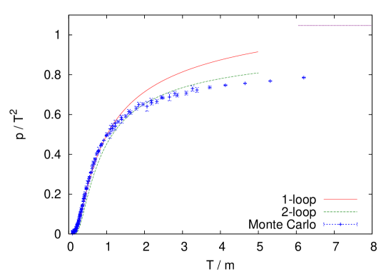
Figure 1: Comparison of the analytic expression for the pressure (the solid line is the one-loop result, the dashed line is the two-loop result) with lattice Monte-Carlo results obtained with the integral method for the case $N=3$. The upper right line marks the Stefan-Boltzmann limit $\pi/3$.

We now turn to the pressure of the system, which is, up to a sign, identical to the minimum of the effective potential: $p=-V_{\mathrm{eff}}^{\mathrm{min}}$. Its renormalized form reads

$$p(T)=N\dfrac{M(T)^{2}}{2g_{ren}^{2}}+N\int_{0}^{\infty}\dfrac{dk}{\pi}\dfrac{k^{2}}{\omega_{k}}\dfrac{1}{\exp\left\{\omega_{k}/T\right\}-1}-N\frac{M(T)^{2}}{8\pi}\left(1+\ln\frac{\mu^{2}}{M^{2}}\right)+N\frac{m^{2}}{8\pi}\text{ .}$$ (7)

Once the pressure is known one can compute the energy density $\rho$ and the trace anomaly $\theta$ using the first principle of thermodynamics: $\rho=Tdp/dT$ , $\theta=\rho-p$ .

The one-loop pressure of Eq. (7) is reported in Fig. 1 and is compared with a lattice study of this system Giacosa (2011) for the case $N=3.$ One can notice that the result is good for small temperatures, but it does not match the lattice data when the temperature increases. This result is indeed expected: the one-loop expression in Eq. (7) reduces to $T^{2}N\pi/6$ for large $T$, which corresponds to a free gas of $N$ non-interacting particles. This result cannot be correct, because the constraint expressed by the $\delta$ function in Eq. (1) eliminates one degree of freedom.

One can go beyond the one-loop results and study the pressure at the two-loop level using the formalism developed in Warringa (2004), see also ref. Giacosa (2011). A better agreement is obtained for large $T,$ although the low-$T$ domain is slightly worsened. Indeed, it is possible to show analytically that for large $T$ the two-loop pressure approaches the correct value $T^{2}(N-1)\pi/6$.

3 Conclusions

In this work we have studied the $O(N)$ model in 1+1 dimensions at nonzero $T.$ We have described how a mass gap is generated for $T=0$, thus demonstrating the occurrence of dimensional transmutation. We have then shown explicitly the analytic results for the pressure at the one-loop level and briefly commented on the results at the two-loop level. Finally, these analytic expressions for the pressure have been compared with lattice results, see Fig. 1.

More advanced analytical calculations can be performed in the future and compared to lattice data: in fact, this system represents a good tool to test nonperturbative approaches, which can then be applied to the more difficult case of Yang-Mills theories in four dimensions.

References

- Novikov (1984) V. A. Novikov, M. A. Shifman, A. I. Vainshtein and V. I. Zakharov, Phys. Rept. 116 (1984) 103 [Sov. J. Part. Nucl. 17 (1986) 204]; Fiz. Elem. Chast. Atom. Yadra 17 (1986) 472.
- Wolff (1990) U. Wolff, Nucl. Phys. B 334 (1990) 581.
- Bruckmann (2008) F. Bruckmann, Phys. Rev. Lett. 100 (2008) 051602 [arXiv:0707.0775 [hep-th]]; J. O. Andersen, D. Boer and H. J. Warringa, Phys. Rev. D 74 (2006) 045028 [hep-th/0602082]; I. Affleck, Phys. Lett. B 92 (1980) 149.
- Hofmann (1995) R. Hofmann, Int. J. Mod. Phys. A 20 (2005) 4123 [hep-th/0504064]; U. Herbst and R. Hofmann, ISRN High Energy Phys. 2012 (2012) 373121 [hep-th/0411214]; F. Giacosa and R. Hofmann, Prog. Theor. Phys. 118 (2007) 759 [hep-th/0609172].
- Pisarski (1981) D. J. Gross, R. D. Pisarski and L. G. Yaffe, Rev. Mod. Phys. 53 (1981) 43.
- Cornwall (1974) J. M. Cornwall, R. Jackiw, and E. Tomboulis, Phys. Rev. D 10 2428 (1974).
- Giacosa (2011) E. Seel, D. Smith, S. Lottini and F. Giacosa, arXiv:1209.4243 [hep-ph].
- Seel (2012) E. Seel, S. Struber, F. Giacosa and D. H. Rischke, arXiv:1108.1918 [hep-ph].
- Mermin (1966) N. D. Mermin and H. Wagner, Phys. Rev. Lett. 17 (1966) 1133; S. R. Coleman, Commun. Math. Phys. 31 (1973) 259.
- Giacosa (2011) F. Giacosa, Phys. Rev. D 83 (2011) 114002 [arXiv:1009.4588 [hep-ph]]; F. Brau and F. Buisseret, Phys. Rev. D 79 (2009) 114007 [arXiv:0902.4836 [hep-ph]]; A. Peshier, B. Kampfer, O. P. Pavlenko and G. Soff, Phys. Rev. D 54 (1996) 2399; P. Castorina and M. Mannarelli, Phys. Rev. C 75 (2007) 054901 [hep-ph/0701206 [hep-ph]].
- Warringa (2004) J. O. Andersen, D. Boer and H. J. Warringa, Phys. Rev. D 69 (2004) 076006 [hep-ph/0309091].