Influence of pions and hyperons on stellar black hole formation

Abstract

We present numerical simulations of stellar core-collapse with spherically symmetric, general relativistic hydrodynamics up to black hole formation. Using the CoCoNuT code, with a newly developed grey leakage scheme for the neutrino treatment, we investigate the effects of including pions and $\Lambda$-hyperons into the equation of state at high densities and temperatures on the black hole formation process. Results show non-negligible differences between the models with reference equation of state without any additional particles and models with the extended ones. For the latter, the maximum masses supported by the proto-neutron star are smaller and the collapse to a black hole occurs earlier. A phase transition to hyperonic matter is observed when the progenitor allows for a high enough accretion rate onto the proto-neutron star. Rough estimates of neutrino luminosity from these collapses are given, too.

I Introduction

Supernovae and hypernovae are among the most spectacular events in the observable universe with an enormous amount of energy involved. Numerous studies have been undertaken to understand their mechanisms, for recent reviews, see e.g. Kotake et al. (2006); Ott (2009); Janka (2012) and references therein. At the origin of an iron core-collapse supernovae is the gravitational collapse of the core of a massive progenitor star exceeding its Chandrasekhar mass. The induced electron captures, reducing the degeneracy pressure of the core, enable the collapse to proceed until the matter density is high enough for nuclear forces to become repulsive. This is the case when, roughly, nuclear matter saturation density has been reached. At this point, a bounce occurs, leaving a compact remnant : a proto-neutron star (PNS), or possibly a black hole (BH).

The bounce creates a shock that propagates outwards and soon stalls, having lost a lot of energy in photodissociation of iron group nuclei within the infalling material. The shock is known to stall in the semi-transparent regime, where the neutrinos are decoupled from the fluid but can still interact. In particular, they deposit energy behind the shock via charged-current interactions. While the collapse, bounce and prompt shock propagation phases seem to be well reproduced by spherically symmetric simulations, it is now widely admitted that the late phases are deeply multidimensional.

Over decades much effort has been devoted to numerical simulations in order to gain physical insight. Increasing computer power and refined models have lead, in recent years, to considerable progress in understanding, in particular, the supernova explosion mechanism using multidimensional models. Indeed, aided by convection (e.g. Murphy and Meakin (2011)) and the standing accretion shock instability (SASI) Blondin and Mezzacappa (2003); Foglizzo et al. (2007), several authors reported explosions by the neutrino heating mechanism in 2D or 3D (e.g. Marek and Janka (2009); Suwa et al. (2010); Bruenn et al. (2009); Takiwaki et al. (2012)). Although some drawbacks still exist, for instance the reported explosion energies are low ($\sim 10^{50}\ \textrm{erg}$ compared with the canonical observed value of $\sim 10^{51}\ \textrm{erg}$), reviving the shock by depositing neutrino energy in the gain layer in a multidimensional simulation seems to be a promising way to finally make the supernovae explode (e.g. Janka (2012); Kotake et al. (2012a)). However, other mechanisms like the acoustic mechanism (e.g. Burrows et al. (2006); Janka (2012)) or the QCD phase transition mechanism Sagert et al. (2009) cannot be excluded. The MHD mechanism (e.g. Obergaulinger et al. (2009); Endeve et al. (2012); Takiwaki and Kotake (2011); Winteler et al. (2012)) could also account for the explosion of rapidly rotating, highly magnetized cores and lead to luminous supernovae or hypernovae.

Black hole formation has been intensely investigated (see e.g. Sumiyoshi et al. (2007); Fischer et al. (2009); O’Connor and Ott (2011); Hempel et al. (2012)). A simulation in which the shock is not able to recover positive velocities and to break through the infalling material from the progenitor leads to the formation of a BH, which often swallows the entire progenitor Ugliano et al. (2012). This is often referred to as a failed supernova. Neutrino emission in failed supernovae simulations stops abruptly when the emission region enters the apparent horizon, as one could expect. This gives a good criterion to discriminate between BH formation and neutron star formation in an upcoming neutrino signal Kotake et al. (2012b). Due to larger accretion rates, failed supernovae simulations are also known to explore higher densities and temperatures than their exploding counterparts, which makes them a tool to explore finite temperature equations of state (EoSs) at supranuclear density.

The EoS remains one of the uncertainties in a stellar core-collapse numerical simulation. The vast majority of simulations employs either the H.Shen et al. EoS (HShen, Shen et al. (1998)) or the Lattimer and Swesty EoS (LS, Lattimer and Swesty (1991)). Both of them assume the same particle content: free nucleons, $\alpha$-particles, one (representative) heavy nucleus, electrons, positrons and photons. Concerning the nuclear interaction, the HShen EoS is based on a relativistic mean field model with a Thomas–Fermi approximation for the description of the inhomogeneous part, while the LS EoS uses a non-relativistic Skyrme-type model with a simplified momentum-independent nucleon-nucleon interaction. The latter EoS is further described in Sec. II.5. EOS dependence has been studied since many years with, in particular, studies of the effects of incompressibility in LS EoS Thompson et al. (2003), or differences between HShen and LS for BH formation Sumiyoshi et al. (2007); Fischer et al. (2009); O’Connor and Ott (2011). More recently, it has been shown Suwa et al. (2012) that differences in the nuclear properties can account for differences in the resulting hydrodynamics, specifically the predicted central density, pressure or compactness of the proto-neutron star. Suwa et al Suwa et al. (2012) have also shown that there is a difference in the gain layer where convection is triggered and the simulations behave differently, qualitatively and quantitatively. These differences can be large enough to govern the presence of an explosion.

Some other finite temperature EoSs are available, especially recent ones (e.g. Hempel et al. (2012); Shen et al. (2011)), focusing on improvements in the subsaturation regime. In this paper, we focus on a different aspect, not included in the standard EoSs, namely the presence of additional particles at high densities and temperatures. It is natural and widely accepted that additional particles should appear in matter at densities above roughly nuclear matter saturation density Lattimer and Prakash (2007). The high temperatures during core-collapse are in favor of the population of these additional states. Supernovae simulations with pions and hyperons added to the HShen EoS were reported in Ishizuka et al. Ishizuka et al. (2008), Sumiyoshi et al Sumiyoshi et al. (2009) and Nakazato et al. Nakazato et al. (2012). The results show in particular that the time from bounce to BH collapse is shortened by the presence of pions and/or hyperons. The neutrino signal is hardly, or not at all changed, except for the fact that the duration of the signal is shorter due to earlier collapse to a BH. The reason is that pions and hyperons appear only deep inside the PNS. Nakazato et al. Nakazato et al. (2012) show in addition that a variation of the coupling parameters of hyperons have only very little influence on these qualitative results. We extend this work to the other commonly used EoS, the LS EoS.

We discuss two extensions of the LS EoS: one including a free pion gas and another one including the $\Lambda$-hyperon. Unfortunately, very few constraints on the interactions of these particles exist, be it from nuclear physics experiments or astronomical observations. The most stringent one at the moment is probably the observation of an almost $2\ \textrm{M}_{\odot}$ neutron star Demorest et al. (2010), a mass measured with high precision by Shapiro delay. Many EoSs including additional particles, in particular hyperons, are in contradiction with this observation due to a too strong softening of the EoS. For instance, with the HShen EoS + $\Lambda$ Shen et al. (2011) only a maximum neutron star mass of $\sim 1.75\ \textrm{M}_{\odot}$ is obtained. With the Ishizuka et al. EoSs Ishizuka et al. (2008), the maximum masses for their EoSs with different parameterizations of hyperons, muons and pions are $1.55,1.63$ and $1.65\ \textrm{M}_{\odot}$. Our extensions of the LS EoS have been described in detail in Oertel et al. (2012), where it was shown in particular that it is possible, including hyperons in the EoS, to fulfill the constraint from the $2\ \textrm{M}_{\odot}$ neutron star measurement together with the available experimental constraints on hyperon couplings. In Sec. II.5 we shall introduce the EoSs models we are employing.

Our simple neutrino treatment does not allow to extract an energy-resolved neutrino signal, we thus only discuss some results for integrated luminosities and we will concentrate the discussion on the time between bounce and black hole collapse as well as on the properties of the different PNSs. The EoS with the $\Lambda$-hyperon shows a phase transition Gulminelli et al. (2012a) to hyperonic matter, whose imprints on the collapse shall be discussed.

This paper is organized as follows. In Sec. II, we review the equations solved by our code and describe the employed finite temperature EoSs. In Sec. III we describe the newly implemented leakage scheme, and then our results are discussed in Sec. IV.

In this paper we use a metric signature $(-,+,+,+)$ and geometrical units in which $c=G=k_{B}=1$. Greek indices run from 0 to 3, while Latin indices run from 1 to 3. We adopt the Einstein summation convention, too.

II Model and equations

We perform a series of numerical simulations using the CoCoNuT code in spherical symmetry. Note that the code can be run in 2D/3D too, but due to the very long simulation times, we restrict ourselves to 1D simulations. Nevertheless, the model and equations presented here could be in principle applied to 2D or 3D cases, without any loss of generality. Since details are already available in the literature Dimmelmeier et al. (2005, 2008); Cordero-Carrión et al. (2009), in this section we only briefly describe the equations solved by the code. The newly implemented neutrino treatment is described in detail in the next section.

II.1 General relativistic hydrodynamics

General relativity (GR) is used through the 3+1 approach (see e.g. Gourgoulhon (2012) and references therein), where the 4-metric $g_{\mu\nu}$ is described by the lapse function $\alpha$, the shift 3-vector $\beta^{i}$ and the spatial 3-metric $\gamma_{ij}$. The line element is then written as

$$\mathrm{d}s^{2}=-\alpha^{2}\mathrm{d}t^{2}+\gamma_{ij}(\mathrm{d}x^{i}+\beta^{i}\mathrm{d}t)(\mathrm{d}x^{j}+\beta^{j}\mathrm{d}t)~{}.$$ (1)

Here we use the isotropic gauge, in which the 3-metric is written as

$$\gamma_{ij}=\Phi^{4}f_{ij}~{},$$ (2)

with $f_{ij}$ denoting the flat-space 3-metric and $\Phi$ the conformal factor. Although this gauge choice is fully valid in spherical symmetry, it is denoted as conformally flat condition (CFC, see Wilson et al. (1996)) in the general case (2D or 3D). This approximation misses some aspects of GR (it does not contain gravitational waves, it cannot exactly describe a Kerr black hole or a rotating fluid configuration), but it has been proven to be a very good approximation in the case of core-collapse simulations Shibata and Sekiguchi (2004); Cerdá-Durán et al. (2005).

Assuming here a perfect fluid with 4-velocity $u^{\mu}$ and baryon number density $n_{b}$, we can define a 4-current as $n_{b}u^{\mu}$. For convenience, CoCoNuT works with the fluid density $\rho=m_{n}n_{b}$, where $m_{n}$ is the neutron mass, so that the 4-current reads

$$J^{\mu}=\rho u^{\mu}~{}.$$ (3)

The stress-energy tensor is given by

$$T^{\mu\nu}=\rho hu^{\mu}u^{\nu}+Pg^{\mu\nu},$$ (4)

with $P$ being the fluid pressure and $h=(e+P)/\rho$ the specific enthalpy; $e$ is here the energy density of the fluid. These two quantities obey local conservation equations

$$\nabla_{\mu}J^{\mu}=0\quad\mathrm{and}\quad\nabla_{\mu}T^{\mu\nu}=0~{},$$ (5)

where $\nabla_{\mu}$ denotes the covariant derivative associated to the 4-metric $g_{\mu\nu}$. The electron fraction $Y_{e}=n_{e}/n_{b}$, electron neutrino fraction $Y_{\nu_{e}}=n_{\nu_{e}}/n_{b}$ and electron antineutrino fraction $Y_{\bar{\nu}_{e}}=n_{\bar{\nu}_{e}}/n_{b}$ enter separately three advection equations, which are included hereafter in a conservative-like form.

No advection equation has been introduced for $Y_{\nu_{x}}$, with $\nu_{x}=\left\{\nu_{\mu},\nu_{\tau},\bar{\nu}_{\mu},\bar{\nu}_{\tau}\right\}$ standing for muon and tau neutrinos. Before bounce, $Y_{\nu_{x}}$ vanishes to a very good approximation, because of the absence of charged-current production processes due to the lack of heavy charged leptons. The only production channels are pair productions (see Sec. III.2.2) which start to play a role in the hot environment close to and after bounce. After bounce, we determine $Y_{\nu_{x}}$ from the integration of the Fermi-Dirac distribution with zero chemical potential for the $\nu_{x}$, thus assuming thermally equilibrated $\nu_{x}$. This simplification saves some computational time and should not have any major influence on our results, since non-electronic neutrinos are much less abundant than electronic ones. Non-electronic neutrinos have thus only little effect on the overall dynamics compared with the electronic ones (see e.g. Liebendörfer et al. (2009), where the dynamics of a full Boltzmann simulation is well reproduced by a simplified simulation with no $\nu_{x}$).

The 3+1 formalism slices the four-dimensional spacetime by three-dimensional spacelike hypersurfaces, and it is therefore particularly well adapted to describe hydrodynamics with respect to a Eulerian observer, which moves orthogonally to these spacelike hypersurfaces with a 4-velocity $n^{\mu}$. The $3+1$ decomposition of the stress-energy tensor reads

$$T^{\mu\nu}=E\,n^{\mu}n^{\nu}+n^{\mu}S^{\nu}+S^{\mu}n^{\nu}+S^{\mu\nu},$$ (6)

$E$ being the matter energy density, $S^{i}$ the matter momentum density, and $S^{ij}$ the matter stress tensor, all measured by the Eulerian observer. Note that the momentum density and the matter stress tensors are orthogonal to the Eulerian observer’s 4-velocity $n^{\mu}$, they can be therefore described as 3-tensors (i.e. using Latin indices) tangent to the spacelike hypersurfaces.

The Eulerian observer sees the fluid with a 3-velocity $v^{i}=u^{i}/(\alpha u^{0})+\beta^{i}/\alpha$. In order to simplify notations, we also introduce the velocity $\hat{v}^{i}=v^{i}-\beta^{i}/\alpha$. To write explicitely the hydrodynamic equations in flux-conservative form Banyuls et al. (1997), we define a set of “conserved” variables

$$D=\rho W,\ \ S^{i}=\rho hW^{2}v^{i},\ \ \mathcal{E}=E-D=\rho hW^{2}-P-D~{},$$ (7)

where $W=\alpha u^{0}=1/\sqrt{1-v_{i}v^{i}}$ is the Lorentz factor.

From Eqs. (5) and (7), adding the three advection equations for $Y_{e},Y_{\nu_{e}},Y_{\bar{\nu}_{e}}$, we then derive flux-conservative hyperbolic Eqs. Banyuls et al. (1997):

$$\frac{\partial\sqrt{\gamma}\bm{U}}{\partial t}+\frac{\partial\sqrt{-g}\bm{F}^{i}}{\partial x^{i}}=\sqrt{-g}\bm{\Sigma},$$ (8)

where

$$\bm{U} = [D,S_{j},\mathcal{E},DY_{e},DY_{\nu_{e}},DY_{\bar{\nu}_{e}}]~{},$$

$$\bm{F}^{i} = [D\hat{v}^{i},S_{j}\hat{v}^{i}+\delta^{i}_{j}P,\mathcal{E}\hat{v}^{i}+Pv^{i},DY_{e}\hat{v}^{i},DY_{\nu_{e}}\hat{v}^{i},DY_{\bar{\nu}_{e}}\hat{v}^{i}]~{},$$

$$\bm{\Sigma} = [0,\frac{T^{\mu\nu}}{2}\frac{\partial g_{\mu\nu}}{\partial x^{j}},T^{00}\left(K_{ij}\beta^{i}\beta^{j}-\beta^{i}\frac{\partial\alpha}{\partial x^{i}}\right)+$$

$$T^{0i}\left(2K_{ij}\beta^{j}-\frac{\partial\alpha}{\partial x^{i}}\right)+T^{ij}K_{ij},$$

$$\Sigma_{e},\Sigma_{\nu_{e}},\Sigma_{\bar{\nu}_{e}}]~{}.$$

$g$ and $\gamma$ are the determinant of $g_{\mu\nu}$ and $\gamma_{\mu\nu}$, respectively, and $K_{ij}$ is the extrinsic curvature, defined by Eq. (12). $\Sigma_{e},\Sigma_{\nu_{e}},\Sigma_{\bar{\nu}_{e}}$ are the creation-annihilation terms that shall be detailed hereafter. These general-relativistic hydrodynamic equations are solved using high-resolution shock-capturing schemes (see e.g. Font (2008) and references therein).

The creation-annihilation terms are computed as follow:

$$\Sigma_{e} = -\Sigma_{ec}+\Sigma_{pc}~{},$$ (9)

$$\Sigma_{\nu_{e}} = \Sigma_{ec}+\Sigma_{ee}+\Sigma_{pl}-\frac{Y_{\nu_{e}}}{t_{esc}}~{},$$ (10)

$$\Sigma_{\bar{\nu}_{e}} = \Sigma_{pc}+\Sigma_{ee}+\Sigma_{pl}-\frac{Y_{\bar{\nu}_{e}}}{t_{esc}}~{},$$ (11)

where $\Sigma_{ec}$ denotes the electron capture rate, $\Sigma_{pc}$ the positron capture rate, $\Sigma_{ee}$ and $\Sigma_{pl}$ the pair annihilation and plasmon decay rates, respectively (defined in Appendix B). We have introduced here the neutrino leak term $Y_{\nu}/t_{esc}$ that represents the number of neutrinos able to reach the neutrinosphere, i.e. able to escape. $t_{esc}$ is the time needed for the neutrinos present at a given radius $r$ to reach the neutrinosphere and is discussed in Sec. III.2.2, too.

Note the following modifications compared with previous work Dimmelmeier et al. (2008):

1. The neutrino pressure no longer appears in the hydrodynamic source terms, Eq. (8). It is instead taken into account together with the other neutrino source terms, see Eq. (33).

2. Two equations for $Y_{\nu_{e}}$ and $Y_{\bar{\nu}_{e}}$ are added to describe neutrino advection.

3. Three sources, $\Sigma_{e},\Sigma_{\nu_{e}}$ and $\Sigma_{\bar{\nu}_{e}}$, are added. $\Sigma_{\nu_{e}}$ and $\Sigma_{\bar{\nu}_{e}}$ track creation and annihilation of neutrinos and, via lepton number conservation, $\Sigma_{e}$ accounts for the changes in the electron fraction.

All these are further detailed in the Sec. III and explicit expressions are given in App. A and App. B. Simulations are performed on a Eulerian grid with spherical geometry. Our spherically symmetric runs have 805 ($r$) points, and a logarithmic grid spacing.

Global convergence of the different parts of the CoCoNuT code have been studied in details in Dimmelmeier et al. (2005). Our new numerical developments, namely the small changes in the hydrodynamics presented here and the leakage scheme, do not modify the convergence properties for the gravitational and hydrodynamics solvers.

II.2 Gravitational potential equations in isotropic gauge

Our treatment of the gravitational potential is similar to Dimmelmeier et al. (2005); Cordero-Carrión et al. (2009). We briefly review here the set of equations solved by lorene Gourgoulhon et al. (1997–2012), a C++ library designed to solve 3+1 GR equations by means of spectral methods Grandclément and Novak (2009). The CoCoNuT code uses this library for solving gravitational field equations through the “marriage des maillages” approach Dimmelmeier et al. (2005).

We start by defining the extrinsic curvature

$$K^{ij}=\frac{1}{2\alpha\Phi^{4}}\left(\mathcal{D}^{i}\beta^{j}+\mathcal{D}^{j}\beta^{i}-\frac{2}{3}f^{ij}\mathcal{D}_{k}\beta^{k}\right),$$ (12)

where $\mathcal{D}_{j}$ is the covariant derivative associated with the flat metric $f_{ij}$. We can then introduce the quantity

$$A^{ij}=\Phi^{10}K^{ij},$$ (13)

and the momentum constraint can be written as

$$\mathcal{D}_{j}A^{ij}=8\pi\Phi^{10}S^{i}=8\pi\Phi^{6}f^{ij}S_{j}=8\pi f^{ij}S_{j}^{*},$$ (14)

with $S_{j}^{*}=\Phi^{6}S_{j}$.

Now, we write $A^{ij}$ as

$$A^{ij}=\mathcal{D}^{i}X^{j}+\mathcal{D}^{j}X^{i}-\frac{2}{3}\mathcal{D}_{k}X^{k}f^{ij},$$ (15)

where $X^{i}$ is a 3-vector (see Cordero-Carrión et al. (2009), too). Combining Eqs. (14) and (15) we get

$$\Delta X^{i}+\frac{1}{3}\mathcal{D}^{i}\mathcal{D}_{j}X^{j}=8\pi f^{ij}S_{j}^{*},$$ (16)

which is the first equation solved by the code to obtain $X^{i}$; we can then deduce $A^{ij}$ thanks to Eq. (15) and solve the Hamiltonian constraint equation

$$\Delta\Phi=-2\pi\Phi^{-1}E^{*}-\Phi^{-7}\frac{f_{il}f_{jm}A^{lm}A^{ij}}{8},$$ (17)

where $E^{*}=\Phi^{6}E$. Knowing the conformal factor, we can solve

$$\Delta(\Phi\alpha)=2\pi\alpha\Phi^{-1}(E^{*}+2S^{*})+\alpha\Phi^{-7}\frac{7f_{il}f_{jm}A^{lm}A^{ij}}{8},$$ (18)

with $S^{*}=\Phi^{6}\gamma_{ij}S^{ij}=\Phi^{6}\left(\rho h(W^{2}-1)+3P\right)$ the conformally rescaled trace of the matter stress tensor. It is thus possible to get the lapse. Then, by solving

$$\Delta\beta^{i}+\frac{1}{3}\mathcal{D}^{i}(\mathcal{D}_{j}\beta^{j})=\mathcal{D}_{j}(2\alpha\Phi^{-6}A^{ij}),$$ (19)

we obtain the shift. Note that this approach is not bound to the spherically-symmetric case (see Cordero-Carrión et al. (2009) in the 3D and CFC case).

II.3 Apparent horizon

We use the apparent horizon (AH) finder described in details in Lin and Novak (2007). In a simulation, a PNS accretes mass and looses energy due to neutrinos at the same time. This enables the PNS to further contract, and consequently the density increases. At some point, depending on the EoS, the PNS becomes gravitationally unstable and collapses to a BH. The BH collapse is unambiguous, as density, temperature, pressure, internal energy all increase very rapidly. Since the lapse is decreasing from $\alpha\simeq 1$ in the Newtonian limit to zero at the center, some authors just take a given value $\alpha\ll 1$ of the lapse as a criterion for BH formation (see e.g. Fischer et al. (2009)). However, using an AH finder that detects a marginally trapped surface is a more rigorous way to treat BH formation. In addition, the AH finder enters a simulation only at the very end, when BH collapse begun, triggered by a chosen value for the conformal factor at the center (typically, $\Phi(r=0)\geq 2$), it is thus computationally cheap.

II.4 Initial models

We employ two different 40 $\textrm{M}_{\odot}$ (zero-age main sequence (ZAMS) mass) progenitors. As a first progenitor model, we have chosen a star with low metalicity ($10^{-4}$ solar) from Woosley, Heger, and Weaver Woosley et al. (2002) (hereafter u40). The low metalicity leads to a much higher accretion rate after bounce compared with a solar metalicity star. Therefore, even though there still are many unknowns concerning the fate of a particular progenitor (see e.g. Ugliano et al. (2012)), very massive stars with low metalicity are widely accepted as good candidates for BH formation.

The second one, from Woosley and Weaver Woosley and Weaver (1995) (hereafter WWs40), has solar metalicity. This progenitor was widely used in BH collapse studies (see e.g. O’Connor and Ott (2011); Fischer et al. (2009); Sumiyoshi et al. (2007); Hempel et al. (2012)) and we use it here mainly for comparison purposes. It is believed to collapse to a BH, as the accretion rate is too high and the iron core is too massive for the star to explode. Let us stress, however, that Ugliano et al Ugliano et al. (2012) report that the $40\ \textrm{M}_{\odot}$ progenitor with solar metalicity from Woosley, Heger, and Weaver Woosley et al. (2002), does explode and leaves a NS rather than a BH. The reason is probably that it has a smaller accretion rate than its counterpart from Woosley and Weaver (1995), a difference that may come from the different treatment of the mass loss.

II.5 Equations of state

In the central region, i.e. mainly within the hot PNS, very high densities (roughly above nuclear saturation) and temperatures (several tens of MeV) are reached. Under these conditions, the particle content of the standard nuclear EoS such as the HShen EoS or the LS EoS is possibly not sufficient. As already mentioned, the latter models the matter as a mixture of one (average) heavy nucleus, $\alpha$-particles, free nucleons, electrons, positrons and photons. Additional particles, such as thermal pions, hyperons, or nuclear resonances should appear. Even a QCD phase transition is conceivable Sagert et al. (2009). In the last years some work in this direction has begun, extending the HShen EoS to include pions or hyperons, see e.g. Sumiyoshi et al. (2009); Ishizuka et al. (2008); Shen et al. (2011), or quarks, see Sagert et al. (2009).

Table 1: Properties of cold neutron stars for the different employed EoSs. The LS180 EoS is added for comparison. The given radii are circumferential ones.

Name	LS180	LS220	LS220+$\Lambda$	LS220 + $\pi$
Maximum gravitational mass [$M_{\odot}$]	1.84	2.06	1.91	1.95
Maximum baryonic mass [$M_{\odot}$]	2.12	2.40	2.22	2.27
Radius at maximum mass [km]	10.13	10.67	9.28	9.94
Radius at $M_{g}=1.4M_{\odot}$ [km]	12.19	12.71	12.41	12.03
Central density at maximum mass [fm-3]	1.26	1.09	1.47	1.26

Here we employ EoSs which are extensions of the other widely used nuclear EoS by Lattimer and Swesty Lattimer and Swesty (1991). Electrons and positrons are treated as non-interacting relativistic gas in pair equilibrium, neglecting electron-screening effects; photons are treated as an ideal ultra-relativistic gas. Equilibrium with respect to strong and electromagnetic interactions is assumed, while $\beta$ equilibrium is not requested, which is consistent with expectations during core-collapse events. Nuclear interaction is treated using a liquid drop model and the transition between inhomogeneous and homogeneous nuclear matter is described via a Maxwell construction. Details can be found in the original paper Lattimer and Swesty (1991).

There are three different sets of parameter values available, resulting in three different values of the nuclear incompressibility, $K=180,220,$ and $375$ MeV. In this work, we restrict ourselves to the value $K=220$ MeV, which gives an EoS compatible with both nuclear data, which suggest a value around $K=240\textrm{MeV}$ (see e.g. Shlomo et al. (2006)), and the recent high mass neutron star of $M=1.97\pm 0.04\ \textrm{M}_{\odot}$ Demorest et al. (2010). The maximum mass of a cold neutron star is 2.06 $\textrm{M}_{\odot}$ (2.40 $\textrm{M}_{\odot}$ baryonic mass) with $K=220$ MeV. The EoS with $K=180$ MeV, on the lower end of possible $K$-values from nuclear data, fails to reproduce the neutron star mass constraint giving a maximum cold neutron star mass of only $1.84\ \textrm{M}_{\odot}$ and $K=375$ MeV lies well above the allowed region from nuclear data. For a thorough comparison of the three different LS EoSs in the context of core collapse simulations, see Suwa et al. (2012).

In Oertel et al. (2012) different possible extensions of the LS EoS are discussed, considering hyperonic degrees of freedom as well as pions and muons. Within this work we limit the discussion to two rather simple cases: one including pions and the other one including the $\Lambda$-hyperon. For the former one, pions have been added upon the LS EoS as a free gas. For a critical discussion of this approximation see Oertel et al. (2012).

The second one, including the $\Lambda$-hyperon can be seen as analogue to the HShen + $\Lambda$ EoS from Shen et al. (2011). The motivation is that the $\Lambda$ represents, together with the $\Sigma^{-}$-hyperon, probably the most important hyperonic degree of freedom in hot dense supernova matter. Thus, including the $\Lambda$ allows for discussing general features of the effects coming from the hyperonic degrees of freedom, without the necessity of resolving the complicated particle composition in the presence of many different hyperons. Indeed, most of them have very low abundances, see e.g. Oertel et al. (2012). The $\Lambda\Lambda$ and the $\Lambda N$ interactions are taken from the model by Balberg and Gal Balberg and Gal (1997) with the parameterization 220BG from Oertel et al. (2012). This model has the advantage of matching well with the LS EoS: in the region where no $\Lambda$-hyperons are present, the interaction is exactly the same as in the LS model.

Within the Balberg and Gal model, the $\Lambda$-hyperons appear through a first order phase transition, see Gulminelli et al. (2012b, a). A Gibbs construction is employed to describe matter in the phase coexistence region, see Gulminelli et al. (2012a) for details. The effect of the criticality of the phase transition on the simulation shall be the subject of forthcoming work.

The maximum gravitational masses of cold neutron stars are $M=1.95\ \textrm{M}_{\odot}$ for the LS220+$\pi$ EoS ($2.27\ \textrm{M}_{\odot}$ baryonic mass) and $M=1.91\ \textrm{M}_{\odot}$ for the LS220+$\Lambda$ EoS ($2.22\ \textrm{M}_{\odot}$ baryonic mass) with parameterization 220BG. The former value lies in the 1$\sigma$-range for the mass constraint from PSR J 1614-2230, the latter is only very slightly below. Properties for cold neutron stars for the different EoSs used within this work are summarized in Table. 1. The LS model with $K=180$ MeV is added for comparison. The circumferential radii at the canonical value of $M=1.4\ \textrm{M}_{\odot}$ vary only very little for the four EoSs, whereas the radii at maximum mass are lower for the EoSs with additional particles, as expected from the softer character of these EoSs.

III Leakage scheme

III.1 Introduction

Neutrino transport is one of the most challenging aspects of modern supernovae simulations. Because the shock stalls in the semi-transparent regime, an accurate neutrino treatment should rely, in principle, on solving the Boltzmann equation. Several authors report on supernovae simulations with neutrino transport, either Newtonian (e.g. Buras et al. (2006); Ott et al. (2008)), or general relativistic (e.g. Liebendörfer et al. (2004); Müller et al. (2010)), but this remains computationally challenging : a simulation with 3D GR hydrodynamics and a (6D) Boltzmann solver is not done yet (see also Kotake et al. (2012b)). The use of simplified models is therefore fairly common. They are used to tackle 3D hydrodynamics simulations Nordhaus et al. (2010), or for parametric studies of black hole collapse, which is known not to require a fully detailed neutrino transport O’Connor and Ott (2011); Ugliano et al. (2012). In this section, we provide details concerning the implementation of our leakage scheme, mostly inspired by Ruffert et al. (1996); Rosswog and Liebendörfer (2003); O’Connor and Ott (2010); Sekiguchi (2010).

The main idea of the leakage scheme is to treat the neutrinos as a fluid component inside the neutrinosphere. Above the latter, neutrinos are considered as free streaming, and only the energy taken away from the fluid needs to be considered. This is achieved by adding terms to the sources of hydrodynamic equations, Eqs. (8). These additional source terms are explicitly given in Appendix A. It is a grey scheme, that defines and works with a mean energy for every neutrino species. The leakage scheme is, by construction, not sufficient to treat the semi-transparent regime nor to revive the shock. On the other hand, it is a simplified model that comes from physical arguments and enables us to run core-collapse simulations within a reasonable amount of time.

III.2 Implementation

III.2.1 Neutrinosphere

The neutrinosphere is the limit where neutrinos decouple from the fluid. This is characterized by an optical depth $\tau$ of the order of unity. We choose to define it as the region where $\tau=2/3$, consistently with the literature (see e.g. Bruenn (1985); O’Connor and Ott (2010)). In order to find the exact position of the neutrinosphere during a simulation, at each time step the opacity is evaluated, using the mean energy of the neutrinos, Eq. (37).

Following Ruffert et al. (1996); Rosswog and Liebendörfer (2003); O’Connor and Ott (2010); Burrows et al. (2006), the neutrino reactions we consider for calculating the opacity are the following (see also App. B for the details of the implementation) :

1. Elastic scattering off a nucleon,

   $$\nu_{i}+N\rightarrow\nu_{i}+N~{},$$ (20)

   where $N=n,p$, and $\nu_{i}$ represents one of the three neutrino species implemented : electron neutrino $\nu_{e}$, electron antineutrino $\bar{\nu}_{e}$ or other species $\nu_{x}$.

2. Elastic scattering off a nucleus,

   $$\nu_{i}+(A,Z)\rightarrow\nu_{i}+(A,Z),$$ (21)

   where $(A,Z)$ is the mean nucleus.

3. Absorption of a $\nu_{e}$ by a neutron

   $$\nu_{e}+n\rightarrow p+e^{-}$$ (22)

   and absorption of a $\bar{\nu}_{e}$ by a proton

   $$\bar{\nu}_{e}+p\rightarrow n+e^{+},$$ (23)

   are taken into account, when no $\beta$-equilibrium is assumed.

4. Elastic scattering off a $\Lambda$

   $$\nu_{i}+\Lambda\rightarrow\nu_{i}+\Lambda~{}.$$ (24)

   We implement the coherent scattering off $\Lambda$-hyperons and take it into account in the opacity calculation, because the hyperon fraction can become quite large at the end of a simulation (see Sec. IV for the hyperon fraction and App. B for the implementation). We study the impact of this newly implemented reaction on our simulations in Sec. IV.3.3

The optical depth is obtained from the total opacity, $\kappa$, by integrating over $r$,

$$\tau=\int_{r}^{\infty}\kappa\ \mathrm{d}r~{}.$$ (25)

Note that this expression implicitly assumes that neutrinos only move along radial rays. In our code, the upper bound of the integral is taken to be the last cell, where we start the integration, then we move inwards. The first cell reaching $\tau\geq 2/3$ is taken to be the neutrinosphere.

As a refinement of this basic leakage scheme, an effective neutrino chemical potential $\mu_{\nu,\mathit{eff}}$ is introduced in the calculation of the different cross sections following Ruffert et al. (1996),

$$\mu_{\nu,\mathit{eff}}=\mu_{\nu,eq}(1-\exp(-\tau))~{},$$ (26)

with $\mu_{\nu,eq}$ being the neutrino chemical potential in $\beta$-equilibrium given by the EoS as $\mu_{\nu,eq}=\mu_{e}+\mu_{p}-\mu_{n}$. For matter completely transparent to neutrinos with a vanishing optical depth, the effective chemical potential goes to zero. In the other extreme case of a very large optical depth, corresponding to matter opaque to neutrinos, the equilibrium value is reached. Thus, it allows partly to correct for deviations from equilibrium in the semi-transparent regime, although the neutrino distribution function is still represented by a Fermi-Dirac distribution.

From a practical point of view, Eq. (26) usually needs very few iterations to converge (no more than 3), given the neutrino effective chemical potential from the previous time step as a first guess. At the beginning of a simulation, $\mu_{\nu,\mathit{eff}}$ is taken to vanish everywhere.

III.2.2 Neutrino creation and advection

Neutrinos are created by electron capture on free protons (see App. B for the details of the implementation)

$$p+e^{-}\rightarrow\nu_{e}+n,$$ (27)

electron capture on nuclei

$$(A,Z)+e^{-}\rightarrow(A,Z-1)+\nu_{e},$$ (28)

positron capture on free neutrons

$$n+e^{+}\rightarrow\bar{\nu}_{e}+p,$$ (29)

electron-positron pair annihilation

$$e^{-}+e^{+}\rightarrow\nu_{i}+\bar{\nu}_{i},$$ (30)

and plasmon decay

$$\tilde{\gamma}\rightarrow\nu_{i}+\bar{\nu}_{i}.$$ (31)

Since they appear only in the very dense regions close to the center, where $\beta$-equilibrium is assumed, no charged-current reactions on $\Lambda$-hyperons are considered.

Let us stress several approximations applied in the treatment of electron and positron captures. We can justify these approximations by the fact that the leakage by itself is a rather crude approximation, and going into further details without a better neutrino treatment may not be relevant or possible.

Following the rates given in Bruenn Bruenn (1985), electron capture on nuclei is cut off due to the assumption of shell closure for a neutron number $N\geq 40$. It has been shown Langanke et al. (2003) that temperature effects smear out the shell structure and that the capture rate on nuclei with $N\geq 40$ is therefore nonzero.

Electron and positron capture are only relevant out of $\beta$-equilibrium, since in equilibrium the creation and absorption terms cancel each other. Within the leakage scheme, however, the equilibration cannot be described as the balance between both would require the knowledge of the distribution function. We therefore take only the creation part into account below a given critical density where $\beta$-equilibrium is assumed. We choose this density to be $1.17\times 10^{12}\mathrm{g}/\mathrm{cm}^{3}$ (see Sec. III.4), which is in agreement with the general finding that $\beta$-equilibrium sets in at a density of the order $\rho\sim 10^{12}\mathrm{g}/\mathrm{cm}^{3}$, see Sec. III.2.3, too.

In the region behind the prompt shock, matter is strongly neutronized, giving very low values of $Y_{e}$. This effect is in general overestimated by leakage schemes (see Fig. 2, or e.g. O’Connor and Ott (2010)), among others due to the fact that the absorption term is absent, which is slowing down electron capture in this region close to $\beta$-equilibrium. In order to avoid the leakage scheme giving (unrealistic) values of $Y_{e}$ below the lowest one available in the EoS, electron capture is blocked below $Y_{e}=0.045$. This allows to follow a simulation during and after the prompt shock propagation

The reaction rates for neutrino creation and absorption enter the sources of the new advection equations related to electron and neutrino number in Eqs. (9)-(11). They are detailed in App. B. We give here the expression for the neutrino escape time $t_{esc}$, defined as in Ruffert et al. (1996):

$$t_{esc}=a_{1}(R_{\nu}-r)\tau~{}.$$ (32)

$R_{\nu}$ is here the radius of the neutrinosphere. Ruffert et al. Ruffert et al. (1996) have set the free parameter $a_{1}$ to $a_{1}=3$, in order to reproduce well data from transport calculations. We keep this value in our implementation (see Sec. III.4).

Since we determine the position of the neutrinosphere at each time step, some neutrinos may be no longer trapped at a given time step. We separately account for these freed neutrinos due to the inward movement of the neutrinosphere. The treatment of energy losses due to escaping neutrinos will be presented in Sec. III.3.

Finally, note that Eq. (32) as well as Eq. (25) do not have GR corrections. Neutrinos follow a straight line (on the grid) while in principle they should follow a null geodesic. This introduces a small numerical error, compared with the overall approximations induced by the usage of a leakage scheme. In particular, the ad hoc factor of $a_{1}=3$ in Eq. (32) is already larger than the GR corrections in Eqs. (32,25) during our simulations. The biggest underestimation of opacities occurs during BH formation, because the neutrinospheres move closer to the center (or to the newly formed apparent horizon). But we note that we are able to reproduce the collapse of the PNS, which is essentially a free fall.

III.2.3 Deviation from thermal equilibrium

During a core collapse event, neutrinos are in general not in thermal equilibrium, which results in a distribution function different from the Fermi-Dirac one, when using a realistic neutrino transport scheme. Only in some very small regions it can be approximated by the latter. The simplicity of the leakage does not allow for determining the correct distribution function, implying that the neutrino number given by integrating the Fermi-Dirac distribution function is not the same as that given by advection and creation-absorption. Within some leakage schemes the neutrino number is chosen to be given by integration of the Fermi-Dirac distribution function, assuming thus thermal equilibrium at all times. We have chosen to compute instead the neutrino fractions from source terms and advection equations. Therefore, the current neutrino number is not necessarily the same as the value at thermal equilibrium, which is taken only as a maximal value, similarly to Sekiguchi (2010).

This choice allows to perform simulations through the collapse and bounce phases, where otherwise the neutrino number would be strongly overestimated. To illustrate this, in Fig. 1 we display the $Y_{e}$-profile at bounce, a few milliseconds before the launch of the shock. The result obtained with our leakage scheme is compared with that employing the so-called Liebendörfer deleptonization (see Liebendörfer (2005)). The latter is a parameterization of full Boltzmann simulations and reproduces thus well a realistic profile. We can see that the result of the leakage is in good agreement with the predicted deleptonization. The deviation is at most around 5%, excepted at the very center where electron captures in the Liebendörfer scheme are slowed down and finally stopped due to the approaching and onset of $\beta$-equilibrium. $Y_{e}$ becomes constant at a value around $0.28$. The leakage scheme, which neglects the absorption term for electron capture cannot reproduce this trend. $Y_{e}$ continues to decrease until the critical density for the onset of $\beta$-equilibrium is reached. Since this density value is adjusted to reproduce the $Y_{e}$-profile as well as possible during neutronization after bounce (see Fig. 2 and discussion below), $Y_{e}$ at the center at bounce is a little low ($Y_{e}\approx 0.22$), but this should not have a significant impact on the overall dynamics (see O’Connor and Ott (2012), too).

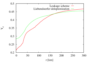
Figure 1: $Y_{e}$ as a function of radius at bounce, using the leakage scheme (plain, red) compared to the Liebendörfer deleptonization prescription (dashed, green)

Fig. 2 shows a comparison of the $Y_{e}$-profile in the leakage scheme with that from the code Agile/Boltztran (from Liebendörfer et al. Liebendörfer et al. (2005)) with a Boltzmann neutrino solver at 10 ms after bounce. This corresponds to the period where matter behind the propagating prompt shock is strongly neutronized. Note that, in order to have the same setting as Liebendörfer et al. (2005), we show here a spherically symmetric simulation with a $15\ \textrm{M}_{\odot}$ progenitor from Woosley and Weaver Woosley and Weaver (1995) with solar metalicity. Moreover, in contrast to all other runs we have performed, the EoS used here is the LS EoS with an incompressibility of $K=180$ MeV, to match the setup of the run with Agile/Boltztran from Liebendörfer et al. (2005).

We observe that, as mentioned above, one of the drawbacks of the leakage scheme is to overestimate the neutronization. The main reason is that the equilibration of electron capture is not correctly described. Otherwise, the leakage scheme is in qualitative agreement with Agile/Boltztran. Note that the irregularities in $Y_{e}$ are due to the different simplifications of the leakage scheme.

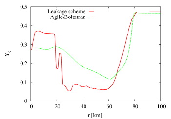
Figure 2: $Y_{e}$-profile during neutronization at $t=10\ \textrm{ms}$ post-bounce using the leakage scheme (plain, red) compared with Agile/Boltztran (dashed, green).

III.3 Treatment of energy losses

In this section, we describe how the energy lost by the fluid, because of neutrino emission, is taken into account. No heating is implemented, as the leakage is not a transport scheme, and therefore no self-consistent derivation of heating sources exist. Moreover, heating does not play a major role in our simulations, given that we expect a collapse to a BH (see discussion in Sec. II.4).

Neutrinos enter the fluid momentum and energy equations as a source term in the equation $\nabla_{\beta}T^{\alpha\beta}=0$,

$$\nabla_{\beta}T^{\alpha\beta}=q^{\alpha},$$ (33)

where we define the source 4-vector $q^{\alpha}$ as

$$q^{\alpha}_{LF}=\left(\begin{array}[]{c}Q_{E}\\ Q_{(M)}^{r}\\ Q_{(M)}^{\theta}\\ Q_{(M)}^{\varphi}\end{array}\right).$$ (34)

If the full neutrino distribution function were known as the solution of the Boltzmann equation, the latter could be employed to build a consistent neutrino stress-energy tensor from which the hydrodynamic sources $q^{\alpha}$ could be derived relying on the condition that the total stress-energy tensor is divergence-free. This has been done in GR by several authors (see e.g. Liebendörfer et al. (2004); Shibata et al. (2011); Müller et al. (2010)), incorporating the energy losses in a coherent way. This is, however, not possible in a leakage scheme, where the energy losses can only be implemented in an approximate way. We follow the choice of O’Connor and Ott (2010) for the vector $q^{\alpha}$, which is detailed below. The quantities in Eq. (34) are defined in the fluid rest frame (or Lagrangian frame, hence the subscript LF), we further need to transform them to the Eulerian frame where the hydrodynamic equations, Eqs. (8), are solved. This transformations are detailed in Appendix A, where the explicit expressions for the source terms used in the code are given as well.

III.3.1 Free streaming regime

In the free streaming regime all neutrinos that are produced leave the simulation, and take away their energy from the fluid. Knowing the neutrino creation rates, $R_{i}$, from each considered reaction, and the mean neutrino energy in each reaction, $\langle\epsilon_{i}\rangle$, (following again Ruffert et al. (1996)), we can write the total rate of energy loss by the fluid in the free streaming regime as follows:

$$Q_{E}=\Sigma_{ec}\langle\epsilon_{ec}\rangle+\Sigma_{pc}\langle\epsilon_{pc}\rangle+\Sigma_{ee}\langle\epsilon_{ee}\rangle+\Sigma_{pl}\langle\epsilon_{pl}\rangle+Q_{freed}~{}.$$ (35)

We have added here to the energy loss by neutrino creation in electron/positron capture, pair annihilation and plasmon decay, the energy loss rate, $Q_{freed}$, due to the freed neutrinos (if any) when the neutrinosphere moves inwards. This term is new and comes from our implementation of advection equations for neutrino fractions. See App. B for further details on the implementation. Note that no momentum is removed from the fluid in the free streaming regime.

III.3.2 Trapped regime

In the trapped regime only those neutrinos reaching the neutrinosphere take away energy. The total energy per unit time lost by the fluid in the trapped regime thus reads

$$Q_{E}=-a_{2}\langle\epsilon_{\nu}\rangle\frac{Y_{\nu}}{t_{esc}}~{},$$ (36)

with the mean energy per particle of escaping neutrinos, $\langle\epsilon_{\nu}\rangle$. In our grey scheme, this mean energy per particle can be evaluated as follows,

$$\langle\epsilon_{\nu}\rangle=\frac{\int_{0}^{\infty}Ef_{FD}(\eta)\mathrm{d}^{3}p}{\int_{0}^{\infty}f_{FD}(\eta)\mathrm{d}^{3}p}=T\frac{F_{3}(\eta)}{F_{2}(\eta)},$$ (37)

where $f_{FD}$ is the Fermi-Dirac distribution function and $F_{k}$ is the Fermi integral of order $k$,

$$F_{k}(\eta)=\int_{0}^{\infty}\mathrm{d}x\ \frac{x^{k}}{1+\exp(x-\eta)}~{}.$$ (38)

$T$ is the temperature and $\eta$ is the degeneracy parameter ($\eta_{\nu}=\mu_{\nu}/T$). Note that since $\langle\epsilon_{\nu}\rangle$ depends on $\eta_{\nu}$, its value is sensitive to the use of the effective chemical potential introduced in Eq. (26).

The energy loss rate, Eq. (36), is calculated separately for each neutrino species considered ($\nu_{e}$, $\bar{\nu}_{e}$, $\nu_{x}$), each one having its own mean energy and its own fraction.

In order to correct partly for the fact that the leakage scheme describes the energy loss only in an approximate way, we choose to vary $a_{2}$ as a free parameter of order unity. It is adjusted to have a mass of the PNS at BH formation comparable with the literature Fischer et al. (2009); O’Connor and Ott (2011). In this paper, we fix $a_{2}$ to the value $a_{2}=1.1$, see Sec. III.4.

In the trapped part, the momentum removed from the fluid is approximated as the gradient of the neutrino pressure, $P_{\nu}$  Müller et al. (2010); O’Connor and Ott (2010). To compute it, neutrinos are assumed to be an ideal Fermi gas of massless particles up to the neutrinosphere. The neutrino pressure then reads

$$P_{\nu}=\frac{4\pi T^{4}}{3(hc)^{3}}(F_{3}(\eta_{\nu})+F_{3}(-\eta_{\nu})).$$ (39)

The term proportional to $F_{3}(\eta_{\nu})$ in Eq. (39) takes into account the $\nu_{e}$ pressure, while the one proportional to $F_{3}(-\eta_{\nu})$ takes into account the $\bar{\nu}_{e}$ pressure. The pressure of $\nu_{x}$ is negligible and therefore not considered.

The momentum taken away from the fluid is then obtained by computing the gradient of $P_{\nu}$ via Dimmelmeier et al. (2008); O’Connor and Ott (2010):

$$Q_{(M)i}=-\frac{\partial P_{\nu}}{\partial x^{i}};$$ (40)

This expression shall be used to derive the neutrino energy-momentum source terms for the hydrodynamic equations in Appendix A.

Note that the components $Q_{(M)i}$ are exactly zero in the free streaming regime.

III.4 Summary of parameter values

Our leakage scheme has three different parameters.

• The $\beta-$equilibrium density is taken to be $1.17\times 10^{12}\ \textrm{g.cm}^{-3}$ throughout this paper. Different authors report $\beta-$equilibrium to set in between $6\times 10^{11}$ and $2\times 10^{12}\ \textrm{g.cm}^{-3}$ Liebendörfer (2005); Janka et al. (2007). Our value is in agreement with this range.

• $a_{1}$, defined by Eq. (32), has the numerical value $a_{1}=3$. We keep the value reported in Ruffert et al. (1996).

• $a_{2}$, defined by Eq. (36), has the numerical value $a_{2}=1.1$. Since this parameter corrects for the incompleteness of the leakage scheme, it has to be close to unity. It is adjusted to have a mass of the PNS at BH formation comparable with the literature Fischer et al. (2009); O’Connor and Ott (2011).

The quantitative values found in our simulations are quite sensitive to these parameters. Namely, a difference of $\pm 10\%$ in the parameter $a_{2}$ leads to a difference in the PNS maximum mass of $\sim 2\%$, which can lead to significantly more time spent in the accreting phase. A difference of $\pm 10\%$ in the $\beta-$equilibrium density does not change the AH detection time, but the maximum density at bounce changes by about $\pm 10\%$. These tests were done with the lsu40 model (see Sec. IV.1).

We note that the overall behavior described in the results (Sec. IV) is robust. We keep in mind that our neutrino treatment is simplified and that a complete Boltzmann solver may give different quantitative values.

IV Results

We use either progenitor u40 or WWs40 (see Sec. II.4), and we employ the LS220 EoS, the LS220+$\pi$ EoS or the LS220+$\Lambda$ EoS (see Sec. II.5). We name our simulations with the name of the EoS (ls, $\pi$, $\Lambda$), followed by that of the progenitor (u40 or WW40). Names and results are summarized in Tab. 2. Simulations are stopped after the AH is formed.

IV.1 Fiducial model

We start by describing the simulation lsu40, using the LS220 EoS with no extra particles and the u40 progenitor from Woosley et al. (2002). This simulation shall serve as a reference run in order to compare with simulations using other EoSs and/or the other progenitor.

Both the collapse and bounce phases are followed using the leakage scheme, which is possible because we solve advection equations for $Y_{\nu_{e}}$ and $Y_{\bar{\nu}_{e}}$ as described in Sec. III.2.3. The bounce is detected at the moment of the shock formation, but, as there is no switch between the different schemes before and after bounce, the exact moment of bounce detection has very little influence on the dynamics (see Scheidegger et al. (2010) for an example of an implementation using a switch at bounce).

After the bounce, the shock is launched and it reaches a distance of about $98$ km from the center before it stalls. Then, the cooling of the material makes the shock slowly recede. At the end of the simulation, before the BH collapse is triggered, the shock remains about $57$ km away from the center and its velocity has increased to $0.35$c. The PNS radius, defined somewhat arbitrarily at the density of $10^{11}\ \textrm{g.cm}^{-3}$ following Müller et al. (2012a), recedes, too: At bounce, it is about $75$ km, then it shrinks slowly to about $45$ km at the onset of the BH collapse.

As depicted in Fig. 3, the PNS collapses at $415$ ms post-bounce, within about 2 ms. The central density increases from $4.6\times 10^{14}\ \textrm{g.cm}^{-3}$ to $1.5\times 10^{15}\ \textrm{g.cm}^{-3}$ and the temperature raises from $4.3\times 10^{11}$ K to $1.3\times 10^{12}$ K. At 416.8 ms post bounce, the apparent horizon is found and the black hole is formed.

The enclosed mass at the onset of BH collapse, measured by evaluating the baryonic mass up to the position of the shock, is $2.55\ \textrm{M}_{\odot}$ (all masses given in this section are baryonic masses). It is a measure (slightly overestimated, because the shock is not exactly at the PNS radius) of the PNS maximum mass, above which it collapses to a BH. This result is consistent with O’Connor and Ott (2011) within $3\%$ (their reported PNS mass is $2.469\ \textrm{M}_{\odot}$).

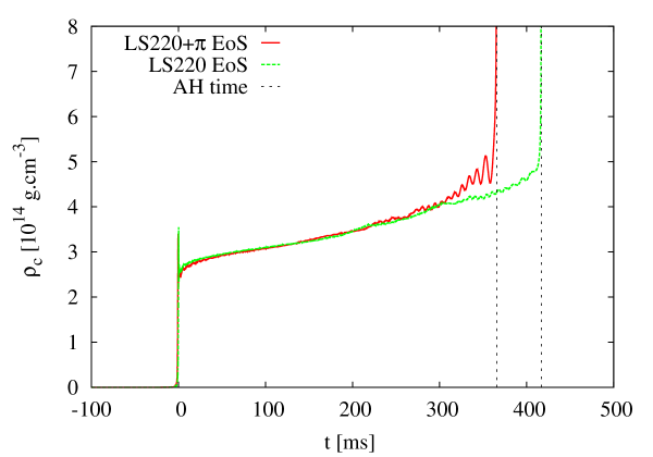
Figure 3: Central density as a function of time post-bounce, for models lsu40 and $\pi$u40. The time corresponding to the first detection of the AH is marked by a vertical line.

IV.2 Model with pions and the u40 progenitor

Adding pions to the EoS slightly softens it, so that we expect the PNS maximum mass and the PNS radius to be slightly smaller.

During the entire simulation, $\pi^{-}$ are the most abundant pions. This is to be expected since negatively charged particles are favored within the neutron rich hot and dense matter encountered during core-collapse. At bounce the maximum of $Y_{\pi^{-}}$ is $Y_{\pi^{-}}=0.0032$. The influence of pions at this moment becomes non-negligible.

In Fig. 3, we can see a consequence of the presence of pions on the collapse phase, namely, the central density at bounce is slightly lower in model $\pi$u40 than in model lsu40. Indeed, collapse and deleptonization are slightly different, and it results in an homologous core and a nascent PNS larger in model $\pi$u40. More precisely, the central temperature is $\sim 2\%$ higher at bounce and the difference stays relatively constant during the first few tens of milliseconds, and this results in a $\sim 3\%$ lower central density for model $\pi$u40 compared to model lsu40.

As can be seen in Fig. 3, the PNS for $\pi$u40 is slightly more compressible and the central density increases more rapidly. At $\sim 200$ ms post-bounce, there is a crossing point where the central densities of both models are the same, then the model with pions predicts a higher density until the collapse to the BH. The addition of pions only slightly changes the behavior after bounce.

The central density in Fig. 3 shows oscillations as it approaches the BH collapse time. We note that these oscillations are more pronounced in model $\pi$u40 than in model lsu40. This might be linked to the higher compressibility of the EoS due to the presence of pions. These oscillations can be damped by medium effects or by multidimensional effects (turbulence, …), and they do not change the qualitative behavior of our simulations, as can be inferred from Fig. 3. So, we think they are not very important for our study.

Fig. 4 shows the pion fraction just before the collapse to the BH at $t=356$ ms post-bounce. As mentioned above, we observe that $\pi^{-}$ are the most abundant, followed by $\pi^{0}$ and then $\pi^{+}$.

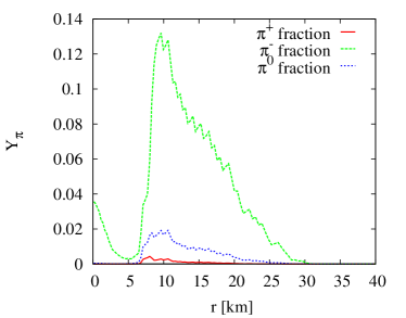
Figure 4: Pion fractions as functions of radius at the onset of BH collapse ($t=356\ \textrm{ms}$ post-bounce, model $\pi$u40). The shape of the profile, in particular the decrease in the central region, is directly correlated with the temperature profile.

We note that $\pi^{-}$ is the only species with a fraction greater than $2\%$, and all species are present only in the very center of the PNS, up to $\sim 30$ km. The shape of the profile, i.e. the fact that near the center the pion fractions are smaller, can be explained by the lower temperature near the center, too. Pions are mainly thermally excited, so that their fractions naturally follow closely the temperature profile. The pion fractions are of the same order as those reported by Nakazato et al. (2012) using an extended HShen EoS. The most abundant species, $\pi^{-}$, has a maximum of $Y_{\pi^{-}}\simeq 0.13$ at the onset of the BH collapse. During a simulation, all pion fractions increase, from 0 to their maximum value at the BH collapse, following the increase of the temperature and the density inside the PNS.

We find that the apparent horizon is detected at 366.3 ms post bounce for a PNS maximum mass of $2.49\ \textrm{M}_{\odot}$ with a PNS radius of 43 km. We note that even though pion fractions are not very large ($Y_{\pi^{-}}$ is the only one over $0.10$, and only in the last tens of milliseconds before BH collapse), this small change in the EoS results in non-negligible changes in the dynamics, especially the time before BH collapse.

IV.3 Model with $\Lambda$-hyperons and the u40 progenitor

IV.3.1 Contraction of the PNS

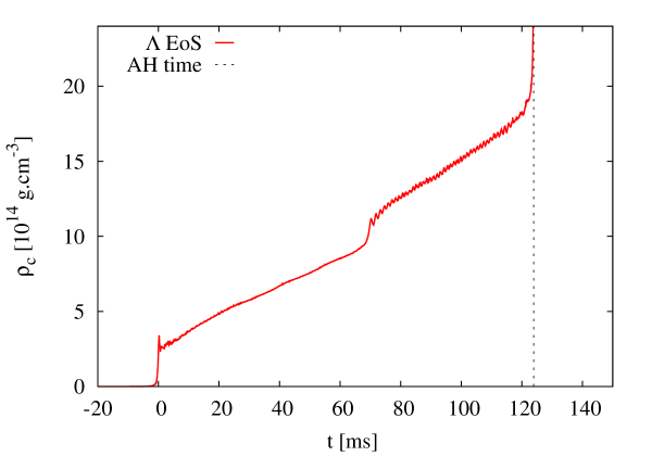
Figure 5: Central density as a function of time post-bounce, for model $\Lambda$u40. The time corresponding to the first detection of the AH is marked by a vertical line.

Adding $\Lambda$-hyperons to the EoS results in a more compact PNS, and the effect is much more pronounced than with pions.

Indeed, in model $\Lambda$u40, the onset of collapse to BH occurs at $122.8$ ms post-bounce and the AH is detected at $123.9$ ms post-bounce, for a maximum mass of the PNS of only $2.00\ \textrm{M}_{\odot}$. Note that this value is significantly lower than its cold EoS counterpart (LS220+$\Lambda$ allows for cold neutron stars with a maximum baryonic mass of $2.22\ \textrm{M}_{\odot}$). This difference might be attributed to dynamical effects. In addition, the hot proto-neutron star is not entirely in $\beta$-equilibrium, such that the $Y_{e}$ profile is given dynamically. Since the EoS depends considerably on $Y_{e}$, this might explain the lower supported mass, too.

Fig. 5 shows that the central density increases much more rapidly than in the fiducial model lsu40. The shock propagates only up to $36$ km away from the center before receding. The newly formed PNS extends to $31$ km a few milliseconds after bounce and contracts to a radius of $17$ km very rapidly. Contraction continues slowly all along the simulation up to the phase transition (described in the next subsection), where the PNS radius suddenly decreases from $15$ km to $13$ km. It further contracts to about $10$ km at the onset of BH collapse. This radius is very small for a hot PNS (see e.g. Müller et al. (2012b) for reported PNS radii with another progenitor and the LS180 EoS. Radii typically lie between $20$ and $70$ km).

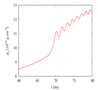
Figure 6: Central density as a function of time post-bounce, model $\Lambda$u40, zoomed on the phase transition.

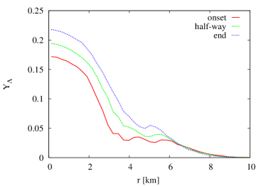
Figure 7: $Y_{\Lambda}$ evolution during phase transition (model $\Lambda$u40). Snapshots are taken at the onset ($t=68.7\ \textrm{ms}$ post-bounce), half-way through ($t=69.5\ \textrm{ms}$ post-bounce) and at the end of the phase transition ($t=70.2\ \textrm{ms}$ post-bounce).

IV.3.2 Phase transition

The LS220+$\Lambda$ EoS contains a first order phase transition to hyperonic matter, as discussed in Sec. II.5, which we expect to find in a core-collapse simulation. Indeed, Fig. 6 is a detailed view of Fig. 5, where a phase transition occurs. The density raises from $9.4\times 10^{14}\ \textrm{g.cm}^{-3}$ to $11.2\times 10^{14}\ \textrm{g.cm}^{-3}$ within less than $2$ ms (around 68-70 ms post-bounce).

This phase transition leads to a sudden contraction of the PNS on a dynamical time scale, as discussed in Sec. IV.3.1. Further contraction of the PNS is very similar to the contraction of the iron core during the initial collapse.

Fig. 7 shows the $\Lambda$-hyperon fraction $Y_{\Lambda}$ as a function of radius during the phase transition. At finite temperature, $\Lambda$-hyperons already appear at bounce, and $Y_{\Lambda}$ keeps increasing to reach $\sim 0.17$ at the center at $68$ ms post-bounce. Then, the phase transition occurs, and we can see in Fig. 7 that $Y_{\Lambda}$ increases from $\sim 0.17$ to $\sim 0.22$ at the center. This happens within less than $2$ ms. After the phase transition, $Y_{\Lambda}$ oscillates with the density and increases again at BH collapse.

Fig. 8 shows $Y_{\Lambda}$ at the onset of BH collapse. We see that $Y_{\Lambda}$ is quite large and can go up to $0.41$ at the very center of the PNS. Note that the phase transition is a consequence of the very large accretion rate of the progenitor, and other progenitors can give a PNS that collapses directly to BH before reaching the region of phase transition (see Sec. IV.4).

Moreover, Fig. 6 shows oscillations of the PNS excited by the collapse at phase transition. These could be fundamental mode radial oscillations of the PNS (see Kokkotas and Ruoff (2001) for a study in cold neutron stars, with different EoSs). It is not possible to directly compare the oscillation frequency of our simulations, which we estimate to be $\sim 800\ \textrm{Hz}$, to the data presented in Kokkotas and Ruoff (2001), because i) the authors discuss only cold neutron stars, ii) our system accretes matter continuously and iii) we use none of the EoSs listed in their tables. Nevertheless, the order of magnitude is correct and given the uncertainties on our estimations of mass and radius of our PNS, we might interpret these oscillations to be the fundamental radial mode of the PNS. In addition, we performed several simulations with increased resolution to rule out a numerical artifact, and we found these oscillations to be robust.

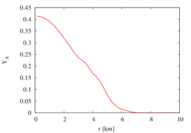
Figure 8: $Y_{\Lambda}$-profile (model $\Lambda$u40) at the onset of BH collapse ($t=121\ \textrm{ms}$ post-bounce).

Table 2: Properties at BH collapse.

Name	lsu40	$\pi$u40	$\Lambda$u40	lsWW40	$\pi$WW40	$\Lambda$WW40
Initial model	u40	u40	u40	WWs40	WWs40	WWs40
EoS	LS220	LS220+$\pi$	LS220+$\Lambda$	LS220	LS220+$\pi$	LS220+$\Lambda$
AH (ms post-bounce)	416.8	366.3	123.9	1025.8	607.2	274.5
PNS mass ($\textrm{M}_{\odot}$)	2.55	2.49	2.00	2.73	2.40	2.00
PNS radius (km)	45	43	10	51	38	18

IV.3.3 Influence of the $\Lambda$-scattering

To test the influence of our newly implemented isoenergetic scattering off $\Lambda$ (see Sec. III.2.1 and App. B), another simulation is conducted using the same parameters and the same EoS, but switching off the $\Lambda$-scattering, and we compare it to the simulation with $\Lambda$-scattering.

Differences are negligible up to the phase transition. Then, without scattering off $\Lambda$, the phase transition occurs $6$ ms later, and the PNS maximum mass becomes $1.96\ \textrm{M}_{\odot}$. This is a reduction of $0.04\ \textrm{M}_{\odot}$ compared with the case including $\Lambda$-scattering. This reduction of the maximum mass suggests that cooling is more important when we reduce the opacity by neglecting scattering off $\Lambda$-hyperons, as expected. However, the reduction is within the error bars of the code, so this conclusion should be taken with some care. We note that although $\Lambda$-hyperons are abundant, they appear in a medium that is already optically thick. This could explain why the $\Lambda$-scattering is not very important.

IV.3.4 Neutrino luminosity

As a complementary tool, we compute the total luminosity $L_{\nu}$. In spherical symmetry, we approximate it by

$$L_{\nu}=4\pi\int_{0}^{\infty}W\left(1+\frac{v_{r}}{\Phi^{2}}\right)\left[\frac{1}{\alpha}-\frac{\beta^{r}}{\alpha}\right]Q_{E}\,\sqrt{-g}\,\mathrm{d}r.$$ (41)

$Q_{E}$ being defined in the fluid rest frame, we have to transform it to the Eulerian frame with a Lorentz boost (with a Eulerian velocity $v_{r}/\Phi^{2}$, see Appendix A), and then to the coordinate frame, which is done by multiplying by the terms in brackets. The generalization to 3D would involve a Lorentz boost in an arbitrary direction and the complete shift vector.

The neutrino luminosity can be found by integrating the energy rate on an invariant volume element at constant time, which justifies the $\sqrt{-g}$ term. This formula agrees with O’Connor and Ott (2010); Kuroda et al. (2012). Note that the integration at constant time is an approximation, since a time delay between the different emitting regions should exist. But because the overall emitting region is narrow ($\sim 100$ km at most), this approximation should be well justified.

As already reported by different authors (e.g., Kuroda et al. (2012); Nakazato et al. (2012)), the total neutrino luminosity peaks at the neutrino burst, a few milliseconds after the bounce, and decreases very rapidly afterwards. We observe the same behavior (see also Fig. 10 and the discussion for the WWs40 progenitor in Sec. IV.4), and the luminosity for models lsu40 and $\pi$u40 are very similar. Only $\Lambda$u40 shows a different trend.

The neutrino burst peak luminosity is higher, and because the PNS shrinks very rapidly, high neutrino emission after bounce is more sustained with the model $\Lambda$u40. As a result, the luminosity decrease after the neutrino burst is slower in this model.

Moreover, after the phase transition the luminosity follows the PNS behavior (illustrated by the central density plot in Fig. 5), and oscillates, which makes the PNS loose a lot of energy. The differences in luminosity between LS220 EoS and $\Lambda$EoS have to be checked with a better neutrino treatment to infer the detectability of the LS220 + $\Lambda$ EoS peculiarities. In addition, the detection of PNS modes could be linked to a physical process different from the phase transition, and it would be hard to disentangle on a neutrino light curve.

Finally, at BH formation, the emitting region enters the horizon and the luminosity drops down abruptly.

IV.4 Results with a WWs40 progenitor

Within this section we discuss simulations performed using a $40\ \textrm{M}_{\odot}$, solar metalicity progenitor from Woosley and Weaver (1995), varying between EoSs LS220, LS220+$\pi$ and LS220+$\Lambda$. This progenitor has often been used to study BH collapse O’Connor and Ott (2011); Fischer et al. (2009); Sumiyoshi et al. (2007); Hempel et al. (2012), as its iron core is reported to be very large. The main difference with the u40 progenitor from Woosley et al. (2002) is that the accretion rate is significantly higher in the latter.

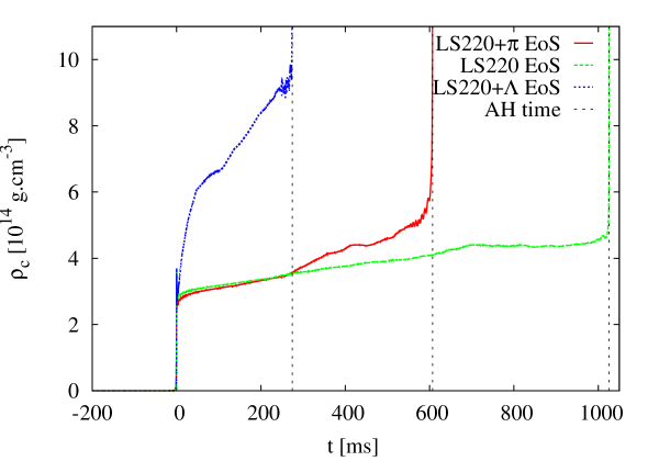
Figure 9: Central density as a function of time for model lsWW40 (dashed, green), $\pi$WW40 (plain, red) and $\Lambda$WW40 (dotted, blue).

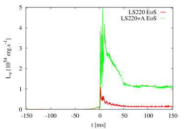
Figure 10: Neutrino luminosity as a function of post-bounce time for model $\Lambda$WW40 (dashed, green), compared to reference model lsWW40 (plain, red). Model $\Lambda$WW40 shows a very high peak luminosity and a more sustained neutrino burst.

In Fig. 9, we observe the same trend as for progenitor u40. With the model $\pi$WW40, the bounce occurs at lower density than with the model lsWW40, and after $275$ ms the curves cross, due to the fact that LS220+$\pi$ EoS allows the PNS to contract faster. For model lsWWs40 we find a maximum PNS mass of $2.73\ \textrm{M}_{\odot}$. Compared with previous work O’Connor and Ott (2011), this value agrees within about $12\%$, and may be slightly overestimated. Other authors Sumiyoshi et al. (2007); Fischer et al. (2009) often use a lower value of the coefficient of nuclear incompressibility, namely $K=180\ \textrm{MeV}$, while we use $K=220\ \textrm{MeV}$. This significantly changes the maximum mass that the PNS can hold and thus, comparisons are more difficult.

The model lsWW40 forms an AH at $1025.8$ ms post-bounce, while the model $\pi$WW40 collapses earlier, and an AH is detected at $607.2$ ms, for a maximum PNS mass of $2.40\ \textrm{M}_{\odot}$. We note that the addition of pions leads to larger changes in the properties at BH collapse for WWs40 than for u40 (see Tab. 2). We may interpret this as follows: because the PNS contracts more when using LS220+$\pi$ EoS, the neutrinosphere is closer to the center and so, cooling is more effective. Because accretion rate is lower with the WWs40 progenitor, more time is needed to reach the PNS maximum mass. Hence, the more effective cooling lasts longer and differences between models using LS220+$\pi$ EoS and LS220 EoS are more pronounced.

Fig. 9 has been translated with the respective bounce time of each model. Note that the bounce happens $\sim 12$ ms earlier for model $\Lambda$WW40, as a small fraction of $\Lambda$ begins to appear ($Y_{\Lambda}\sim 0.0005$ at the center at bounce) before bounce. For this model BH collapse is triggered before the phase transition density is reached. Indeed, with progenitor u40 we reach a central density of $10^{15}\ \textrm{g.cm}^{-3}$ at $\sim 69$ ms post-bounce, which triggers the onset of the phase transition. Here, as can be seen in Fig. 9, the collapse to the BH has already started when we reach a density of $10^{15}\ \textrm{g.cm}^{-3}$. This is due to the higher accretion rate of progenitor u40, which allows for higher central densities of the PNS. Hence, the LS220+$\Lambda$ EoS does not induce a phase transition for every progenitor that collapses to a BH. Note that, even without phase transition, we find a non-negligible fraction of $\Lambda$-hyperons ($Y_{\Lambda}\sim 0.15$ at the center at the onset of BH collapse, at $t=271\ \textrm{ms}$ post-bounce. See Fig. 7, too, which shows $Y_{\Lambda}\sim 0.17$ at the center in model $\Lambda$u40 before the phase transition). This is, as noted in Sec. IV.3.2, due to the fact that $\Lambda$-hyperons begin to appear before the phase transition at finite temperature, and their fraction increases with increasing temperature.

Finally, Fig. 10 shows the total neutrino luminosity $L_{\nu}$ (summed over all neutrino species) around the time of neutrino burst. Model $\Lambda$WW40 shows a high peak luminosity of $5.10^{54}\ \textrm{erg.s}^{-1}$, compared to the reference model lsWW40 that shows a maximum of $1.10^{54}\ \textrm{erg.s}^{-1}$. In the model $\Lambda$WW40, the neutrino burst is also longer in time due to the rapid shrinking of the PNS, and the post-bounce luminosity stays higher until BH formation.

V Conclusion

We have presented simulations of stellar core-collapses to BH, comparing different finite-temperature EoSs with additional particles, namely pions and $\Lambda$-hyperons. As expected, additional degrees of freedom modify the EoS properties, in such a way that the collapse to a black hole occurs sooner after the bounce.

Our new EoSs are based on the Lattimer and Swesty EoS. Pions are added as a free gas, and $\Lambda$-hyperons are incorporated with the interactions adapted from Balberg and Gal Balberg and Gal (1997). This EoS is subject to a first-order phase transition driven by $\Lambda$-hyperons Gulminelli et al. (2012b, a) which is described by a Gibbs construction. The LS220+$\pi$ EoS fulfills the gravitational mass constraint from the $M=1.97\pm 0.04\ \textrm{M}_{\odot}$ neutron star, and the LS220+$\Lambda$ EoS is very slightly below with a maximum mass of $1.91\ \textrm{M}_{\odot}$. Compared to previous works, H.Shen et al. Shen et al. (2011) reported a maximum mass of $1.75\ \textrm{M}_{\odot}$ for their EoS including $\Lambda$-hyperons, and Ishizuka et al. Ishizuka et al. (2008) reported a maximum mass of $1.55,1.63$ and $1.65\ \textrm{M}_{\odot}$ for their EoSs that include different parameterizations of hyperons, muons and pions. So, the EoSs presented in this paper are in better agreement with observational mass constraints.

We have implemented a new leakage scheme. Compared with previous works, we keep track of the neutrino fractions more accurately with advection equations, and take into account neutrinos that are not trapped anymore because of the neutrinosphere moving inwards. Although our fluid rest frame source terms are approximated, we consistently transform them to the Eulerian frame, where the hydrodynamic equations are solved. With these refinements, it is possible to follow a simulation during the collapse, bounce and post-bounce phases without changing the approach.

When using the LS220+$\Lambda$ EoS, we have implemented for the first time the isoenergetic scattering off a $\Lambda$-hyperon. It is done in a simplified manner consistent with our other opacity sources, and we find that it shifts the occurrence of the phase transition by $6$ ms and the PNS maximum baryonic mass is $0.04\ \textrm{M}_{\odot}$ smaller with this opacity taken into account. This contribution is still very subdominant compared with scattering off nucleons.

Our use of the leakage scheme during the collapse phase enabled us to see differences in the deleptonization, which resulted in a smaller density at bounce for model $\pi$u40 and $\pi$WW40, compared to lsu40 and lsWW40, respectively. With both progenitors, we find, as expected, that the compression of the PNS is faster when using the LS220+$\pi$ EoS. The reduction of the PNS maximum baryonic mass is $0.06\ \textrm{M}_{\odot}$ for model $\pi$u40 compared to model lsu40. A larger difference of $0.33\ \textrm{M}_{\odot}$ is found when comparing models $\pi$WW40 and lsWW40. We interpret the larger difference as a result of the larger amount of time spent in the post-bounce cooling regime. Small differences between EoSs have thus more time to develop.

With the u40 progenitor and the LS220+$\Lambda$ EoS, a phase transition clearly appears. Contrary to the cold $\Lambda$ EoS, at finite temperature $\Lambda$-hyperons begin to appear before the phase transition, and the fraction of thermally populated $\Lambda$-hyperons is significant ($\sim 0.17$ at the center before the phase transition). The phase transition results in a sudden increase in density, comparable to the free fall during the initial collapse.

In contrast to model $\Lambda$u40, with model $\Lambda$WW40 we do not observe the phase transition. We find that up to the onset of BH collapse, the density stays too low to trigger the phase transition. Consequently, the appearance of $\Lambda$-hyperons is entirely due to thermal effects. We conclude that our models with LS220+$\Lambda$ EoS do not predict a phase transition for every progenitor. Indeed, only the progenitors with the highest accretion rates are able to reach the phase transition density before the onset of BH collapse.

Apart from the lack of the phase transition, the WWs40 progenitor has the same qualitative behavior as u40. Our results with model lsWW40 are in agreement with previous work with the same progenitor and the same EoS O’Connor and Ott (2011). The LS220+$\pi$ EoS collapses to BH earlier than the LS220 EoS, admitting a lower PNS maximum mass. LS220+$\Lambda$ EoS also leads to a more compressible PNS, and the effect is much more pronounced. The PNS maximum mass is found to be $2.00\ \textrm{M}_{\odot}$.

Thus, we addressed the question of additional particles in hot EoSs. It seems that adding pions or $\Lambda$-hyperons can significantly change the conditions of a core-collapse supernova, while still being in agreement with the $M=1.97\pm 0.04\ \textrm{M}_{\odot}$ neutron star. Because we see differences already at bounce, and because the neutrino luminosity is higher when adding $\Lambda$-hyperons, one could infer that additional particles may make a difference in the explosion phase. This will have to be investigated with a more detailed neutrino treatment.

The present EoS with $\Lambda$-hyperons is only marginally compatible with the mass of PSR J 1614-2230 and the question arises to which extent our results would be modified by taking another EoS giving a higher maximum neutron star mass. As far as the same model is used, e.g. with one of the parameter sets from Ref. Oertel et al. (2012), no qualitative changes are to be expected. Indeed, as can be seen from Ref. Oertel et al. (2012), the behavior of the hyperonic EoS with different parameterizations are very similar. More pronounced modifications are of course to be expected if a future observation gives an even higher neutron star mass and another model has to be used (remind that LS220 EoS without additional particles has a maximum mass of only 2.06 M_⊙). The general effect of reduced time to black hole collapse in presence of additional particles seems, however, very robust, since we confirm the results from Ishizuka et al. (2008); Sumiyoshi et al. (2009); Nakazato et al. (2012) which have been obtained using an extended version of the HShen EoS, thus a different model for dense matter.

Further studies on observational consequences of the appearance of hyperons or pions are yet to be done. In particular, the phase transition should produce copious amount of gravitational waves, as it has been shown by previous studies on “mini-collapses” Lin et al. (2006); Dimmelmeier et al. (2009). A future study shall use simulations of rotating stellar core collapse with pion and hyperon EoS, in order to infer the gravitational wave signal. On the other hand, our estimation of neutrino luminosity suggests that the PNS radial modes might be detectable, although it would be hard to unambiguously associate it to a phase transition to hyperonic matter, also because other phase transitions (e.g. to quark matter Sagert et al. (2009)) are possible. So, it seems possible to detect evidences of the phase transition in an ideal case, combining observations of neutrinos and gravitational waves from core-collapse to a BH, even without constraining the nature of the phase transition from these data.

Our work on modern EoSs including pions and $\Lambda$-hyperons raises the question of the impact of the other additional particles that we did not consider. In the long run, it will be desirable to build an EoS with $\pi$, $\Lambda$ but also other hyperons ($\Sigma$, $\Xi$), and muons. This EoS would have to fulfill the mass constraint and consistently take into account interactions between particles. Coupling it to an accurate neutrino transport scheme, taking into account neutrino reactions with the new particles is the only way to have accurate quantitative results on the influence of additional particles. In the mean time, modern nuclear and astrophysical data should restrict more and more the set of compatible parameters, which will help building a realistic EoS.

Appendix A Explicit derivation of the hydrodynamic sources

Neutrinos enter the fluid momentum and energy equations as a source term in the hydrodynamic Eqs. $\nabla_{\beta}T^{\alpha\beta}=q^{\alpha}$, see Eqs. (33, 34). The quantities in Eq. (34) being defined in the Lagrangian frame (LF), we further need to transform them in the Eulerian frame (EF), where the hydrodynamic equations, Eqs. (8), are solved.

We adopt the same conventions as Gourgoulhon (2012) and Müller et al. (2010) for the definitions of frames : The coordinate frame (that can be associated with the grid) is fixed, and its tetrad $\partial_{\mu}$ is used to define the metric $g_{\mu\nu}$ as (see Gourgoulhon (2012))

$$g_{\mu\nu}=\bm{g}(\partial_{\mu},\partial_{\nu}).$$ (42)

Note also that the coordinate frame is not associated with a physical observer. The Eulerian frame is then defined as in Sec. II.1 (the Eulerian observer moves orthogonally to spacelike hypersurfaces). It is an inertial frame, in which the basis vectors span the Minkowski metric $\eta_{\alpha\beta}=\textrm{diag}(-1,1,1,1)$, so that it is only in the Newtonian limit that the Eulerian frame becomes the same as the coordinate frame.

This justifies that the transformation from the LF to the EF is a Lorentz boost and contains no metric terms. Note, however, that our velocity $v_{i}$ defined in Sec. II.1 is written in the coordinate frame, and we need to transform it into the EF.

To do so, we define the matrix of a general Lorentz transformation (tetrad transformation) $P_{\mu}\,^{\nu}$ as

$$g_{\mu\nu}P_{\alpha}\,^{\mu}P_{\beta}\,^{\nu}=\eta_{\alpha\beta}.$$ (43)

Going from the coordinate frame velocity to the EF velocity is done by applying this transformation matrix $P$ to the 4-vector $v^{\mu}=(0,v^{i})$. In the CFC, this simply results in multiplying $v_{i}$ by $\textrm{diag}(1/\Phi^{2},1/(\Phi^{2}r),1/(\Phi^{2}r\sin\theta))$.

Writing the boost for an arbitrary Eulerian velocity $v_{i,EF}=\left(v_{r},v_{\theta},v_{\phi}\right)$ leads to

$$q^{\alpha}_{EF}=\Lambda^{\alpha}\,_{\beta}(v^{i,EF})q^{\beta}_{LF}$$ (44)

and explicitly, the covariant components are

$$q_{0,EF}=W(Q_{E}+v^{i,EF}Q_{(M)i})$$ (45)

$$q_{1,EF}=v_{r}WQ_{E} + \left[1+(W-1)\frac{v_{r}v^{r}}{v_{i}v^{i}}\right]Q_{(M)1}$$ (46)

$$+ \left[(W-1)\frac{v_{r}v^{\theta}}{v_{i}v^{i}}\right]Q_{(M)2}$$

$$+ \left[(W-1)\frac{v_{r}v^{\phi}}{v_{i}v^{i}}\right]Q_{(M)3}$$

$$q_{2}=v_{\theta}WQ_{E} + \left[(W-1)\frac{v_{\theta}v^{r}}{v_{i}v^{i}}\right]Q_{(M)1}$$ (47)

$$+ \left[1+(W-1)\frac{v_{\theta}v^{\theta}}{v_{i}v^{i}}\right]Q_{(M)2}$$

$$+ \left[(W-1)\frac{v_{\theta}v^{\phi}}{v_{i}v^{i}}\right]Q_{(M)3}$$

$$q_{3,EF}=v_{\phi}WQ_{E} + \left[(W-1)\frac{v_{\phi}v^{r}}{v_{i}v^{i}}\right]Q_{(M)1}$$ (48)

$$+ \left[(W-1)\frac{v_{\phi}v^{\theta}}{v_{i}v^{i}}\right]Q_{(M)2}$$

$$+ \left[1+(W-1)\frac{v_{\phi}v^{\phi}}{v_{i}v^{i}}\right]Q_{(M)3}$$

It can easily be seen that Eqs. (45), (46), (47), (48) reduce to the usual spherically symmetric boost by imposing $v_{\theta}=v_{\phi}=0$. Terms arising from the deviation from spherical symmetry, while usually small, can become non-negligible, for instance in the case of a rapidly rotating core Müller et al. (2010).

Finally, in Eq. (8), $q_{0,EF}$ enters as such in the source term of the conserved quantity $\mathcal{E}$ corresponding to the conservation of energy, and $q_{j,EF}$ enters as such in the source term of the conserved quantity $S_{j}$ corresponding to the conservation of momentum. Note that because of the definition of Eq. (8), we recover there a multiplicative metric term, $\sqrt{-g}$.

Appendix B Neutrino reactions formulae

In this appendix, we do not use $c=1$ for clarity. The temperature $T$ is in units of energy.

B.1 Opacities

B.1.1 Elastic scattering off a proton

The opacity $\tau_{s}(\nu p)$ is defined following Ruffert et al. Ruffert et al. (1996), with the cross section corresponding to the transport cross section from Burrows et al. Burrows et al. (2006).

$$\tau_{s}(\nu p)=C_{sp}n_{p}\sigma_{0}\left(\frac{T}{m_{e}c^{2}}\right)^{2}Y_{NN}\frac{F_{5}(\eta_{\nu})}{F_{3}(\eta_{\nu})}~{},$$ (49)

where $n_{p}$ is the proton number density, $T$ is the temperature, $\eta_{\nu}$ is the degeneracy parameter, and $\sigma_{0}$ is the weak interaction cross section, defined by

$$\sigma_{0}=\frac{4(m_{e}c^{2}G_{F})^{2}}{\pi(\hbar c)^{4}}~{},$$ (50)

with $G_{F}$ being the Fermi constant, $m_{e}$ the electron mass, and $F_{p}$ the Fermi integral of order $p$ defined by Eq. (38). The $F_{5}/F_{3}$ term comes from phase space integration and corresponds to the energy opacities in Ruffert et al. (1996), which are the ones we find in better agreement with more detailed calculations. We also include the following approximation for the nucleon-nucleon degeneracy factor $Y_{NN}$,

$$Y_{NN}=\frac{Y_{N}}{1+\frac{2}{3}\max(\frac{\mu_{N}}{T},0)}~{},$$ (51)

where $Y_{N}$ is the nucleon fraction, $\mu_{N}$ is the nucleon chemical potential and $T$ is the temperature. Finally, the constant term $C_{sp}$ takes the value

$$C_{sp}=\frac{1}{24}\left[4(C_{V}-1)^{2}+5\left(\frac{g_{A}}{g_{V}}\right)^{2}\right]~{},$$ (52)

where $g_{V}$ and $g_{A}$ are the vector and axial coupling constants of the weak interaction, and $C_{V}=\frac{1}{2}+2\sin^{2}\theta_{W}$ with $\theta_{W}$ the Weinberg angle.

B.1.2 Elastic scattering off a neutron

Following Ruffert et al. Ruffert et al. (1996), the opacity $\tau_{s}(\nu n)$ for the elastic scattering off a neutron is

$$\tau_{s}(\nu n)=C_{sn}n_{n}\sigma_{0}\left(\frac{T}{m_{e}c^{2}}\right)^{2}Y_{NN}\frac{F_{5}(\eta_{\nu})}{F_{3}(\eta_{\nu})}~{},$$ (53)

where $n_{n}$ is the neutron number density. The constant $C_{sn}$ takes the value

$$C_{sn}=\frac{1}{24}\left[1+5\left(\frac{g_{A}}{g_{V}}\right)^{2}\right]~{}.$$ (54)

B.1.3 Elastic scattering off a nucleus

We follow Rampp and Janka Rampp and Janka (2002) here, and define the opacity $\tau_{s}(\nu A)$ as

$$\tau_{s}(\nu A) = \frac{\sigma_{0}A^{2}T^{2}}{16m_{e}c^{2}}n_{A}\frac{F_{5}(\eta_{\nu})}{F_{3}(\eta_{\nu})}$$ (55)

$$\times \left((C_{A}-C_{V})+(2-C_{A}-C_{V})\frac{2Z-A}{A}\right)^{2}$$

$$\times \frac{y_{b}-1+(1+y_{b})\textrm{e}^{-2y_{b}}}{y_{b}^{2}}\langle S(\epsilon)\rangle_{ion}~{},$$

where $n_{A}$ is the heavy nuclei number density, and $C_{A}=\frac{1}{2}$. The ion screening term $\langle S(\epsilon)\rangle_{ion}$ is taken into account as in Horowitz Horowitz (1997) and $y_{b}$ is defined as in Bruenn and Mezzacappa Bruenn and Mezzacappa (1997) and Rampp and Janka Rampp and Janka (2002), explicitely

$$y_{b}=\frac{2}{5(\hbar c)^{2}}(1.07A)^{2/3}\langle\epsilon_{\nu}\rangle^{2}~{},$$ (56)

with $A$ the mass number of the average heavy nucleus, and $\langle\epsilon_{\nu}\rangle$ the mean neutrino energy, defined by Eq. 37.

B.1.4 Absorption of a $\nu_{e}$ by a neutron

The opacity $\tau_{a}(\nu_{e}n)$, from Ruffert et al. (1996), for this reaction is

$$\tau_{a}(\nu_{e}n) = \frac{n_{n}}{4}\left[1+3\left(\frac{g_{A}}{g_{V}}\right)^{2}\right]\sigma_{0}|V_{ud}|^{2}\left(\frac{T}{m_{e}c^{2}}\right)^{2}$$ (57)

$$\times \frac{F_{5}(\eta_{\nu_{e}})}{F_{3}(\eta_{\nu_{e}})}\left[1+\exp\left(\eta_{e}-\frac{F_{5}(\eta_{\nu_{e}})}{F_{4}(\eta_{\nu_{e}})}\right)\right]^{-1}$$

with $\eta_{e}$ the degeneracy parameter of the electrons and $|V_{ud}|$ the CKM matrix element.

B.1.5 Absorption of a $\bar{\nu}_{e}$ by a proton

The opacity $\tau_{a}(\bar{\nu}_{e}p)$, from Ruffert et al. (1996), for this reaction is

$$\tau_{a}(\bar{\nu}_{e}p) = \frac{n_{p}}{4}\left[1+3\left(\frac{g_{A}}{g_{V}}\right)^{2}\right]\sigma_{0}|V_{ud}|^{2}\left(\frac{T}{m_{e}c^{2}}\right)^{2}$$ (58)

$$\times \frac{F_{5}(\eta_{\bar{\nu}_{e}})}{F_{3}(\eta_{\bar{\nu}_{e}})}\left[1+\exp\left(-\eta_{e}-\frac{F_{5}(\eta_{\bar{\nu}_{e}})}{F_{4}(\eta_{\bar{\nu}_{e}})}\right)\right]^{-1}$$

B.1.6 Elastic scattering off a $\Lambda$-hyperon

Following the same approximations as for the transport cross section for coherent scattering off neutrons in Bruenn (1985); Ruffert et al. (1996); Burrows et al. (2006) we obtain,

$$\sigma_{\Lambda}=\frac{\sigma_{0}}{4}\left(\frac{1+5c_{A_{\Lambda}}^{2}}{6}\right)~{}.$$ (59)

The constant $c_{A_{\Lambda}}$ is the $\Lambda$ axial coupling constant to the neutral current and is assumed to take its value given by flavor $SU(3)$ symmetry, $c_{A_{\Lambda}}=-0.73$ Savage and Walden (1997); Reddy et al. (1998).

Explicitely, the opacity $\tau_{s}(\nu\Lambda)$ for this reaction is

$$\tau_{s}(\nu\Lambda)=n_{\Lambda}\sigma_{\Lambda}\left(\frac{T}{m_{e}c^{2}}\right)^{2}\frac{F_{5}(\eta_{\nu})}{F_{3}(\eta_{\nu})}~{},$$ (60)

where $n_{\Lambda}$ is the $\Lambda$-hyperon number density. Note that we do not take into account a degeneracy factor in this case.

B.2 Neutrino creation terms

B.2.1 Electron and positron captures

To take into account electron and positron captures, we integrate the following expression (see Bruenn (1985))

$$\Sigma=\frac{c}{n_{b}}\frac{4\pi}{(hc)^{3}}\int_{0}^{\infty}E^{2}j(1-f)\mathrm{d}E~{},$$ (61)

where $\Sigma=\Sigma_{ec},\Sigma_{pc}$; $f$ is the neutrino distribution function, which we assume is a Fermi-Dirac, because no deviation from equilibrium is computed in the leakage scheme. Note that we do not take into account the absorption term, and rather set $\beta$-equilibrium at a given density.

These integrated rates are computationally expensive, and only require the knowledge of the EoS to be computed. Therefore, they can be tabulated as a function of $\rho,T,Y_{e}$ (at each point of the EoS), and the effective neutrino chemical potential $\mu_{\nu,\mathit{eff}}$. Access to the tables is done by a quadrilinear interpolation.

$j$ is the creation term, also taken from Bruenn Bruenn (1985).

B.2.2 Electron capture on free protons

The total electron capture rate is the sum of the electron capture rate on free protons and the electron capture rate on nuclei. For electron capture on free protons, $j_{ec,p}$ takes the value

$$j_{ec,p} = \frac{G_{F}^{2}}{\pi(\hbar c)^{4}}|V_{ud}|^{2}\eta_{pn}(g_{V}^{2}+3g_{A}^{2})f_{e}(E+Q)$$ (62)

$$\times (E+Q)^{2}\left[1-\left(\frac{m_{e}c^{2}}{E+Q}\right)^{2}\right]^{1/2}~{},$$

where $Q$ is the mass difference between neutrons and protons, and $\eta_{pn}$ is such that

$$\eta_{pn}=\int 2\frac{\mathrm{d}^{3}p}{(2\pi)^{3}}f_{n}(E)(1-f_{p}(E))~{},$$ (63)

with $f_{e}$, $f_{n}$ and $f_{p}$ the distribution functions of the electrons, neutrons and protons, respectively, all taken to be Fermi-Dirac distribution functions.

B.2.3 Electron capture on nuclei

For electron capture on nuclei, $j_{ec,n}$ takes the value

$$j_{ec,n} = \frac{G_{F}^{2}}{\pi(\hbar c)^{4}}n_{A}|V_{ud}|^{2}g_{A}^{2}N_{p}(Z)N_{h}(N)f_{e}(E+Q^{\prime})$$ (64)

$$\times (E+Q^{\prime})^{2}\left[1-\left(\frac{m_{e}c^{2}}{E+Q^{\prime}}\right)^{2}\right]^{1/2}~{},$$

with the approximation $Q^{\prime}=\mu_{n}-\mu_{p}+\Delta$, $\mu_{n}$ and $\mu_{p}$ being the neutron and proton chemical potential, respectively, and taking the constant value $\Delta=3\ \textrm{MeV}$.

$N_{p}(Z)$ and $N_{h}(N)$ are also taken following Bruenn Bruenn (1985),

$$N_{p}(Z)=\left\{\begin{array}[]{cc}0,&Z<20\\ Z-20,&20<Z<28\\ 8,&Z>28\end{array}\right.$$ (65)

$$N_{h}(N)=\left\{\begin{array}[]{cc}6,&N<34\\ 40-N,&34<N<40\\ 0,&N>40\end{array}\right.$$ (66)

We start the integration Eq. (61) at the threshold $E=m_{e}c^{2}-Q^{\prime}$ if this value is positive.

B.2.4 Positron capture on free neutrons

For positron capture on free neutrons, $j_{pc}$ takes the value

$$j_{pc} = \frac{G_{F}^{2}}{\pi(\hbar c)^{4}}|V_{ud}|^{2}\eta_{np}(g_{V}^{2}+3g_{A}^{2})f_{e^{+}}(E-Q)$$ (67)

$$\times (E-Q)^{2}\left[1-\left(\frac{m_{e}c^{2}}{E-Q}\right)^{2}\right]^{1/2}~{},$$

where $f_{e^{+}}$ is again a Fermi-Dirac distribution function. $\eta_{np}$ can be inferred from the definition of $\eta_{pn}$ by interchanging $n$ and $p$. We start the integration Eq. (61) at the threshold $E=Q+m_{e}c^{2}$.

B.2.5 Electron positron pair annihilation

Following Ruffert et al. Ruffert et al. (1996),

$$\Sigma_{ee}=C_{ee}\frac{\sigma_{0}c}{(m_{e}c^{2})^{2}}\epsilon_{e^{-}}\epsilon_{e^{+}}\langle 1-f_{\nu_{i}}\rangle_{ee}\langle 1-f_{\bar{\nu}_{i}}\rangle_{ee}~{},$$ (68)

with the definition

$$\epsilon_{e^{\mp}}=\frac{8\pi}{(hc)^{3}}T^{4}F_{3}(\pm\eta_{e})~{},$$ (69)

and the average Fermi distributions

$$\langle 1-f_{\nu_{i}}\rangle_{ee}=\left(1+\exp\left[-\left(\frac{F_{4}(\eta_{e})}{2F_{3}(\eta_{e})}+\frac{F_{4}(-\eta_{e})}{2F_{3}(-\eta_{e})}-\eta_{\nu_{i}}\right)\right]\right)^{-1}$$ (70)

The constant $C_{ee}$ takes the value $C_{ee}=((C_{V}-C_{A})^{2}+(C_{V}+C_{A})^{2})/36$ for $\nu_{e}$ and $\bar{\nu}_{e}$, and $C_{ee}=((C_{V}-C_{A})^{2}+(C_{V}+C_{A}-2)^{2})/9$ for $\nu_{x}$.

B.2.6 Plasmon decay

Following Ruffert et al. Ruffert et al. (1996),

$$\Sigma_{pl} = \frac{\pi^{2}}{3\alpha_{em}}C_{pl}^{2}\frac{\sigma_{0}c}{(m_{e}c^{2})^{2}}\frac{T^{8}}{(hc)^{6}}$$ (71)

$$\times \gamma^{6}\mathrm{e}^{-\gamma}(1+\gamma)\langle 1-f_{\nu_{i}}\rangle_{\gamma}\langle 1-f_{\bar{\nu}_{i}}\rangle_{\gamma}~{},$$

where $\alpha_{em}$ is the fine structure constant, $\gamma$ is defined by

$$\gamma=2\left(\sqrt{\frac{\alpha_{em}}{3\pi}}\right)^{-1}\sqrt{\frac{1}{3}(\pi^{2}+3\eta_{e}^{2})}~{},$$ (72)

and the average Fermi distributions are

$$\langle 1-f_{\nu_{i}}\rangle_{\gamma}=\left(1+\exp\left[-\left(1+\frac{\gamma^{2}}{2(1+\gamma)}-\eta_{\nu_{i}}\right)\right]\right)^{-1}$$ (73)

Note here that $\nu_{x}$ are taken into account with a degeneracy of 4 and a vanishing chemical potential. The constant $C_{pl}$ takes the value $C_{pl}=C_{V}$ for $\nu_{e}$ and $\bar{\nu}_{e}$, and $C_{pl}=C_{V}-1$ for $\nu_{x}$.

References

- Kotake et al. (2006) K. Kotake, K. Sato, and K. Takahashi, Rep. Prog. Phys. 69, 971 (2006).
- Ott (2009) C. D. Ott, Class. Quantum Grav. 26, 204015 (2009).
- Janka (2012) H.-T. Janka, Ann. Rev. Nucl. Part. Sci. (2012), accepted for publication, arXiv:1206.2503.
- Murphy and Meakin (2011) J. W. Murphy and C. Meakin, Astrophys. J. 742, 74 (2011).
- Blondin and Mezzacappa (2003) J. M. Blondin and A. Mezzacappa, Astrophys. J. 584, 971 (2003).
- Foglizzo et al. (2007) T. Foglizzo, P. Galletti, L. Scheck, and H.-T. Janka, Astrophys. J. 654, 1006 (2007).
- Marek and Janka (2009) A. Marek and H.-T. Janka, Astrophys. J. 694, 664 (2009).
- Suwa et al. (2010) Y. Suwa, K. Kotake, T. Takiwaki, S. C. Whitehouse, M. Liebendörfer, and K. Sato, Proc. Astron. Soc. Jap. 62, L49 (2010).
- Bruenn et al. (2009) S. W. Bruenn, A. Mezzacappa, W. R. Hix, J. M. Blondin, P. Marronetti, O. E. B. Messer, C. J. Dirk, and S. Yoshida, J. Phys. Conf. Ser. 180, 012018 (2009).
- Takiwaki et al. (2012) T. Takiwaki, K. Kotake, and Y. Suwa, Astrophys. J. 749, 98 (2012).
- Kotake et al. (2012a) K. Kotake, T. Takiwaki, Y. Suwa, W. Iwakami Nakano, S. Kawagoe, Y. Masada, and S.-i. Fujimoto, Adv. Astron. (2012a), accepted for publication, arXiv:12042330.
- Burrows et al. (2006) A. Burrows, E. Livne, L. Dessart, C. D. Ott, and J. Murphy, New Astron. Rev. 50, 487 (2006).
- Sagert et al. (2009) I. Sagert, T. Fischer, M. Hempel, G. Pagliara, J. Schaffner-Bielich, A. Mezzacappa, F.-K. Thielemann, and M. Liebendörfer, Phys. Rev. Lett. 102, 081101 (2009).
- Obergaulinger et al. (2009) M. Obergaulinger, P. Cerdá-Durán, E. Müller, and M. A. Aloy, Astron. Astrophys. 498, 241 (2009).
- Endeve et al. (2012) E. Endeve, C. Y. Cardall, R. D. Budiardja, S. W. Beck, A. Bejnood, R. J. Toedte, A. Mezzacappa, and J. M. Blondin, Astrophys. J. 751, 26 (2012).
- Takiwaki and Kotake (2011) T. Takiwaki and K. Kotake, Astrophys. J. 743, 30 (2011).
- Winteler et al. (2012) C. Winteler, R. Käppeli, A. Perego, A. Arcones, N. Vasset, N. Nishimura, M. Liebendörfer, and F.-K. Thielemann, Astrophys. J. Lett. 750, L22 (2012).
- Sumiyoshi et al. (2007) K. Sumiyoshi, S. Yamada, and H. Suzuki, Astrophys. J. 667, 382 (2007).
- Fischer et al. (2009) T. Fischer, S. C. Whitehouse, A. Mezzacappa, F.-K. Thielemann, and M. Liebendörfer, Astron. Astrophys. 499, 1 (2009).
- O’Connor and Ott (2011) E. O’Connor and C. D. Ott, Astrophys. J. 730, 70 (2011).
- Hempel et al. (2012) M. Hempel, T. Fischer, J. Schaffner-Bielich, and M. Liebendörfer, Astrophys. J. 748, 70 (2012).
- Ugliano et al. (2012) M. Ugliano, H.-T. Janka, A. Marek, and A. Arcones, Astrophys. J. (2012), accepted for publication, arXiv:1205.3657.
- Kotake et al. (2012b) K. Kotake, K. Sumiyoshi, S. Yamada, T. Takiwaki, T. Kuroda, Y. Suwa, and H. Nagakura, Prog. Theor. Phys. (2012b), accepted for publication, arXiv:1205.6284.
- Shen et al. (1998) H. Shen, H. Toki, K. Oyamatsu, and K. Sumiyoshi, Nucl. Phys. A 637, 435 (1998).
- Lattimer and Swesty (1991) J. M. Lattimer and F. D. Swesty, Nucl. Phys. A 535, 331 (1991).
- Thompson et al. (2003) T. A. Thompson, A. Burrows, and P. A. Pinto, Astrophys. J. 592, 434 (2003).
- Suwa et al. (2012) Y. Suwa, T. Takiwaki, K. Kotake, T. Fischer, M. Liebendörfer, and K. Sato (2012), arXiv:1206.6101.
- Shen et al. (2011) G. Shen, C. J. Horowitz, and S. Teige, Phys. Rev. C 83, 035802 (2011).
- Lattimer and Prakash (2007) J. M. Lattimer and M. Prakash, Phys. Rep. 442, 109 (2007).
- Ishizuka et al. (2008) C. Ishizuka, A. Ohnishi, K. Tsubakihara, K. Sumiyoshi, and S. Yamada, J. Phys. G 35, 085201 (2008).
- Sumiyoshi et al. (2009) K. Sumiyoshi, C. Ishizuka, A. Ohnishi, S. Yamada, and H. Suzuki, Astrophys. J. Lett. 690, L43 (2009).
- Nakazato et al. (2012) K. Nakazato, S. Furusawa, K. Sumiyoshi, A. Ohnishi, S. Yamada, and H. Suzuki, Astrophys. J. 745, 197 (2012).
- Demorest et al. (2010) P. Demorest, T. Pennucci, S. Ransom, M. Roberts, and J. Hessels, Nature 467, 1081 (2010).
- Shen et al. (2011) H. Shen, H. Toki, K. Oyamatsu, and K. Sumiyoshi, Astrophys. J. Suppl. 197, 20 (2011).
- Oertel et al. (2012) M. Oertel, A. F. Fantina, and J. Novak, Phys. Rev. C 85, 055806 (2012).
- Gulminelli et al. (2012a) F. Gulminelli, A. Raduta, M. Oertel, and J. Margueron (2012a), eprint in preparation.
- Dimmelmeier et al. (2005) H. Dimmelmeier, J. Novak, J. A. Font, J. M. Ibáñez, and E. Müller, Phys. Rev. D 71, 064023 (2005).
- Dimmelmeier et al. (2008) H. Dimmelmeier, C. D. Ott, A. Marek, and H.-T. Janka, Phys. Rev. D 78, 064056 (2008).
- Cordero-Carrión et al. (2009) I. Cordero-Carrión, P. Cerdá-Durán, H. Dimmelmeier, J. L. Jaramillo, J. Novak, and E. Gourgoulhon, Phys. Rev. D 79, 024017 (2009).
- Gourgoulhon (2012) E. Gourgoulhon, 3+1 Formalism in General Relativity: Bases of Numerical Relativity, vol. 846 of Lecture Notes in Physics (Springer, Berlin; New York, 2012).
- Wilson et al. (1996) J. R. Wilson, G. J. Mathews, and P. Marronetti, Phys. Rev. D 54, 1317 (1996).
- Shibata and Sekiguchi (2004) M. Shibata and Y. Sekiguchi, Phys. Rev. D 69, 084024 (2004).
- Cerdá-Durán et al. (2005) P. Cerdá-Durán, G. Faye, H. Dimmelmeier, J. A. Font, J. M. Ibáñez, E. Müller, and G. Schäfer, Astron. Astrophys. 439, 1033 (2005).
- Liebendörfer et al. (2009) M. Liebendörfer, S. C. Whitehouse, and T. Fischer, Astrophys. J. 698, 1174 (2009).
- Banyuls et al. (1997) F. Banyuls, J. A. Font, J. M. Ibáñez, J. M. Martí, and J. A. Miralles, Astrophys. J. 476, 221 (1997).
- Font (2008) J. A. Font, Living Rev. Relat. 11, 7 (2008).
- Gourgoulhon et al. (1997–2012) E. Gourgoulhon, P. Grandclément, J.-A. Marck, and J. Novak, LORENE: Langage Objet pour la RElativité NumériquE, http://www.lorene.obspm.fr (1997–2012).
- Grandclément and Novak (2009) P. Grandclément and J. Novak, Living Rev. Relat. 12, 1 (2009).
- Lin and Novak (2007) L.-M. Lin and J. Novak, Class. Quantum Grav. 24, 2665 (2007).
- Woosley et al. (2002) S. E. Woosley, A. Heger, and T. A. Weaver, Rev. Mod. Phys. 74, 1015 (2002).
- Woosley and Weaver (1995) S. E. Woosley and T. A. Weaver, Astrophys. J. Suppl. 101, 181 (1995).
- Shlomo et al. (2006) S. Shlomo, V. M. Kolomietz, and G. Colò, Eur. Phys. J. A 30, 23 (2006).
- Balberg and Gal (1997) S. Balberg and A. Gal, Nucl. Phys. A625, 435 (1997).
- Gulminelli et al. (2012b) F. Gulminelli, A. Raduta, and M. Oertel, Phys. Rev. C 86, 025805 (2012b).
- Buras et al. (2006) R. Buras, M. Rampp, H.-T. Janka, and K. Kifonidis, Astron. Astrophys. 447, 1049 (2006).
- Ott et al. (2008) C. D. Ott, A. Burrows, L. Dessart, and E. Livine, Astrophys. J. 685, 1069 (2008).
- Liebendörfer et al. (2004) M. Liebendörfer, O. E. B. Messer, A. Mezzacappa, S. W. Bruenn, C. Y. Cardall, and F.-K. Thielemann, Astrophys. J. Suppl. 150, 263 (2004).
- Müller et al. (2010) B. Müller, H.-T. Janka, and H. Dimmelmeier, Astrophys. J. Suppl. 189, 104 (2010).
- Nordhaus et al. (2010) J. Nordhaus, A. Burrows, A. Almgren, and J. Bell, Astrophys. J. 720, 694 (2010).
- Ruffert et al. (1996) M. Ruffert, H.-T. Janka, and G. Schäfer, Astron. Astrophys. 311, 532 (1996).
- Rosswog and Liebendörfer (2003) S. Rosswog and M. Liebendörfer, Mon. Not. R. Astron. Soc. 342, 673 (2003).
- O’Connor and Ott (2010) E. O’Connor and C. D. Ott, Class. Quantum Grav. 27 (2010).
- Sekiguchi (2010) Y. Sekiguchi, Class. Quantum Grav. 27, 114107 (2010).
- Bruenn (1985) S. W. Bruenn, Astrophys. J. Suppl. 58, 771 (1985).
- Langanke et al. (2003) K. Langanke, G. Martínez-Pinedo, J. M. Sampaio, D. J. Dean, W. R. Hix, O. E. Messer, A. Mezzacappa, M. Liebendörfer, H.-T. Janka, and M. Rampp, Phys. Rev. Lett. 90, 241102 (2003).
- Liebendörfer (2005) M. Liebendörfer, Astrophys. J. 633, 1042 (2005).
- O’Connor and Ott (2012) E. O’Connor and C. D. Ott (2012), submitted to Astrophys. J., arXiv:1207.1100.
- Liebendörfer et al. (2005) M. Liebendörfer, M. Rampp, H.-T. Janka, and A. Mezzacappa, Astrophys. J. 620, 840 (2005).
- Shibata et al. (2011) M. Shibata, K. Kiuchi, Y. Sekiguchi, and Y. Suwa, Prog. Theor. Phys. 125, 1255 (2011).
- Janka et al. (2007) H.-T. Janka, K. Langanke, A. Marek, G. Martínez-Pinedo, and B. Müller, Phys. Rep. 442, 38 (2007).
- Scheidegger et al. (2010) S. Scheidegger, R. Käppeli, S. C. Whitehouse, T. Fischer, and M. Liebendörfer, Astron. Astrophys. 514, A51 (2010).
- Müller et al. (2012a) B. Müller, H.-T. Janka, and A. Marek, Astrophys. J. 756, 84 (2012a).
- Müller et al. (2012b) E. Müller, H.-T. Janka, and A. Wongwathanarat, Astron. Astrophys. 537, A63 (2012b).
- Kokkotas and Ruoff (2001) K. D. Kokkotas and J. Ruoff, Astron. Astrophys. 366, 565 (2001).
- Kuroda et al. (2012) T. Kuroda, K. Kotake, and T. Takiwaki, Astrophys. J. 755, 11 (2012).
- Lin et al. (2006) L.-M. Lin, K. S. Cheng, M.-C. Chu, and W.-M. Suen, Astrophys. J. 639, 382 (2006).
- Dimmelmeier et al. (2009) H. Dimmelmeier, M. Bejger, P. Haensel, and J. L. Zdunik, Mon. Not. R. Astron. Soc. 396, 2269 (2009).
- Rampp and Janka (2002) M. Rampp and H.-T. Janka, Astron. Astrophys. 396, 361 (2002).
- Horowitz (1997) C. J. Horowitz, Phys. Rev. D 55, 4577 (1997).
- Bruenn and Mezzacappa (1997) S. W. Bruenn and A. Mezzacappa, Phys. Rev. D 56, 7529 (1997).
- Savage and Walden (1997) M. J. Savage and J. Walden, Phys. Rev. D 55, 5376 (1997).
- Reddy et al. (1998) S. Reddy, M. Prakash, and J. M. Lattimer, Phys. Rev. D 58, 013009 (1998).