Long-Time Asymptotics for the Korteweg–de Vries Equation with Steplike Initial Data

Abstract.

We apply the method of nonlinear steepest descent to compute the long-time asymptotics of the Korteweg–de Vries equation with steplike initial data.

1. Introduction

We study the long-time asymptotic behavior of solutions of the Korteweg–de Vries (KdV) equation

(1.1) $$q_{t}(x,t)=6q(x,t)q_{x}(x,t)-q_{xxx}(x,t),\quad(x,t)\in\mathbb{R}\times\mathbb{R},$$

with steplike initial data $q(x,0)=q(x)\in C^{11}(\mathbb{R})$ such that

(1.2) $$\left\{\begin{array}[]{ll}q(x)\to 0,&\ \ \mbox{as}\ \ x\to+\infty,\\ q(x)\to-c^{2},&\ \ \mbox{as}\ \ x\to-\infty,\end{array}\right.$$

moreover,

(1.3) $$\int_{0}^{+\infty}\mathrm{e}^{C_{0}x}(|q(x)|+|q(-x)+c^{2}|dx<\infty,\ \ \ C_{0}>c>0,$$

(1.4) $$\int_{\mathbb{R}}(x^{6}+1)|q^{(i)}(x)|dx<\infty,\quad i=1,...,11.$$

It is known (cf. [15], [16]), that this Cauchy problem has a unique solution satisfying $q(\cdot,t)\in C^{3}(\mathbb{R})$ and

(1.5) $$\int_{0}^{+\infty}|x|(|q(x,t)|+|q(-x,t)+c^{2}|)dx<\infty,\qquad t\in\mathbb{R}.$$

In fact, by [30] it will be even real analytic, but we will not use this fact. From several results ([3]–[8], [19], [20], [17], [29]), obtained on a physical level of rigor, it is known that the asymptotic behavior of $q(x,t)$ as $t\to\infty$ can be split into three main regions:

• In the region $x<-6c^{2}t$ the solution is asymptotically close to the background $-c^{2}$ up to a decaying dispersive tail.

• In the region $-6c^{2}t<x<4c^{2}t$ the solution can asymptotically be described by an elliptic wave.

• In the region $4c^{2}t<x$ the solution is asymptotically given by a sum of solitons.

This is illustrated in Figure 1.

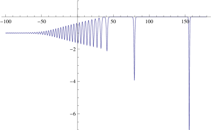
Figure 1. Numerically computed solution $q(x,t)$ of the KdV equation at time $t=10$, with initial condition $q(x,0)=\frac{1}{2}(\mathrm{erf}(x)-1)-5\mathop{\mathrm{sech}}(x-1)$.

In fact, the long-time asymptotics for this problem were first studied by Gurevich and Pitaevskii [19], [20]. These authors have used the Whitham multi-phase averaging method and obtained the main term of the asymptotics of the solution in terms the Jacobi elliptic function. Moreover, they gave a qualitative picture of the splitting of an initial step into solitons. Since the Schrödinger operator with the Heaviside step function as potential has no discrete spectrum, this picture refuted the general idea that solitons arise only from the discrete spectrum. This phenomenon was explained by Khruslov [21], [22] with the help of the inverse scattering transform (IST) in the form of the Marchenko equation. The IST not only made it possible to obtain an explicit form of these asymptotic solitons but also to give a rigorous proof that the solitons are generated by a small vicinity of the edge of the continuous spectrum. Further developments of this method can be found in [32] and [23]. The first finite-gap description of the asymptotics for the steplike initial problem of the KdV equation was given by Bikbaev and Novokshenov [6] only in 1987 (see also [3]–[5], [8], [7], and the review [29]). The results are based on an analysis of the Whitham equations and the theory of analytic functions on a hyperelliptic surface. Our aim here is to use the nonlinear steepest decent method for oscillatory Riemann–Hilbert problem (see [18] for an introduction to this method in the case $c=0$ as well as for further references) and apply it to rigorously establish the above mentioned asymptotics. Related results for an expansive step ($-c^{2}>0$) can be found in [27].

The paper is organized as follows: Section 2 provides some necessary information about the inverse scattering transform on steplike backgrounds. Then we establish the asymptotics in the soliton region $4c^{2}t<x$ in Section 3. In Section 4 the initial RH problem is reduced to a ”model” problem in the domain $-6c^{2}t<x<4c^{2}t$, and in Section 5 we solve this model problem. Section 6 contains the solution of the model problem in the domain $x<-6c^{2}t$.

Finally, we should remark that our results do not cover the two transitional regions: $4c^{2}t\approx x$ near the leading wave front, and $x\approx-6c^{2}t$ near the back wave front. It can be observed numerically that in the first transitional region the modulated elliptic wave develops into a train of asymptotic solitons. As pointed out before, these asymptotic solitons have already been rigorously studied by Khruslov [22]. As for the second region, the matching of the leading asymptotics behind the back front and in the elliptic region for the modified KdV equation is briefly discussed in [24, Rem. 4.3]. However, since the error bounds obtained from the RHP method break down near the edges, a rigorous justification is beyond the scope of the present paper.

2. Statement of the RH problem and the first conjugation step

Let $q(x,t)$ be the solution of the Cauchy problem (1.1)–(1.4). Associated with $q(x,t)$ is a self-adjoint Schrödinger operator

(2.1) $$H(t)=-\frac{d^{2}}{dx^{2}}+q(.,t),\qquad\mathfrak{D}(H)=H^{2}(\mathbb{R})\subset L^{2}(\mathbb{R}).$$

Here $L^{2}(\mathbb{R})$ denotes the Hilbert space of square integrable (complex-valued) functions over $\mathbb{R}$ and $H^{k}(\mathbb{R})$ the corresponding Sobolev spaces.

The spectrum of $H$ consists of an absolutely continuous part $[-c^{2},\infty)$ plus a finite number of eigenvalues $-\kappa_{j}^{2}\in(-\infty,-c^{2})$, $1\leq j\leq N$, where $c<\kappa_{1}<...<\kappa_{N}$. In turn, the absolutely continuous part of the spectrum consists of the part $[0,\infty)$ of multiplicity two and the part $[-c^{2},0]$ of multiplicity one. In addition, there exist two Jost solutions $\phi(k,x,t)$ and $\phi_{1}(k,x,t)$ which solve the differential equation

(2.2) $$H(t)\psi(k,x,t)=k^{2}\psi(k,x,t),\qquad\mathop{\mathrm{Im}}(k)>0,$$

and asymptotically look like the free solutions of the background equations

(2.3) $$\lim_{x\to+\infty}\mathrm{e}^{-\mathrm{i}kx}\phi(k,x,t)=1,\quad\lim_{x\to-\infty}\mathrm{e}^{\mathrm{i}k_{1}x}\phi_{1}(k,x,t)=1.$$

Here $k_{1}=\sqrt{k^{2}+c^{2}}$, and $k_{1}>0$ for $k\in[0,\mathrm{i}c)_{r}$. The last notation means the right side of the cut along the interval $[0,\mathrm{i}c]$. Accordingly, $k_{1}<0$ for $k\in[0,\mathrm{i}c)_{l}$, i.e. from the left. As a function of $k$ the function $\phi(k,x,t)$ (resp., $\phi_{1}$) is analytic in the domain $\mathbb{C}^{U}=\{k:\ \mathop{\mathrm{Im}}(k)>0\}$ (resp. $\mathbb{C}^{U}_{c}:=\mathbb{C}^{U}\setminus(0,\mathrm{i}c]$) and continuous up to the boundary of this domain. Here subscript $U$ corresponds to the upper half plane.

The Jost solutions admit the usual representation via the transformation operators

(2.4) $$\phi(k,x,t)=\mathrm{e}^{\mathrm{i}kx}+ \int_{x}^{+\infty}K(x,y,t)\mathrm{e}^{\mathrm{i}ky}dy,$$

$$\phi_{1}(k,x,t)=\mathrm{e}^{-\mathrm{i}k_{1}x}+ \int^{x}_{-\infty}K_{1}(x,y,t)\mathrm{e}^{-\mathrm{i}k_{1}y}dy,$$

where $K(x,y,t)$ and $K_{1}(x,y,t)$ are real valued functions, and

(2.5) $$K(x,x,t)=\frac{1}{2}\int_{x}^{+\infty}q(y,t)dy,\quad K_{1}(x,x,t)=\frac{1}{2}\int^{x}_{-\infty}(q(y,t)+c^{2})dy.$$

Furthermore, one has the scattering relations

(2.6) $$T(k,t)\phi_{1}(k,x,t)= \overline{\phi(k,x,t)}+R(k,t)\phi(k,x,t),\qquad k\in\mathbb{R},$$

$$T_{1}(k,t)\phi(k,x,t)= \overline{\phi_{1}(k,x,t)}+R_{1}(k,t)\phi_{1}(k,x,t),\qquad k_{1}\in\mathbb{R},$$

where $T(k,t)$, $R(k,t)$ (resp. $T_{1}(k,t)$, $R_{1}(k,t)$) are the right (resp. left) transmission and reflection coefficients. They constitute the entries of the scattering matrix. Denote by

(2.7) $$W(k,t)=\phi_{1}(k,x,t)\phi^{\prime}(k,x,t)-\phi_{1}^{\prime}(k,x,t)\phi(k,x,t)$$

the Wronskian of the Jost solutions, where $f^{\prime}=\frac{\partial}{\partial x}f$. In what follows we assume that the initial data (1.2) belong to the generic class of nonresonant potentials for which

(2.8) $$W(\mathrm{i}c,0)\neq 0.$$

Lemma 2.1 ([10], [15]).

The entries of the scattering matrix have the following properties:

1. The transmission coefficients $T(k,t)$, $T_{1}(k,t)$ are meromorphic in the domain $\mathbb{C}^{U}_{c}:=\mathbb{C}^{U}\setminus(0,\mathrm{i}c]$, continuous up to the boundary and have simple poles at $\mathrm{i}\kappa_{1},\dots,\mathrm{i}\kappa_{N}$. The residues of $T(k,t)$ are given by

   (2.9) $$\operatorname{Res}_{\mathrm{i}\kappa_{j}}T(k,t)=\mathrm{i}\mu_{j}(t)\gamma_{j}(t)^{2},\ \mbox{where}\ \gamma_{j}(t)^{-1}=\lVert\phi(\mathrm{i}\kappa_{j},.,t)\rVert_{2},$$

   and $\phi(\mathrm{i}\kappa_{j},x,t)=\mu_{j}(t)\phi_{1}(\mathrm{i}\kappa_{j},x,t)$.

2. Everywhere in the domain $\mathbb{C}^{U}_{c}$

   (2.10) $$T(k,t)=2\mathrm{i}kW^{-1}(k,t),\ \ T_{1}(k,t)=2\mathrm{i}k_{1}W^{-1}(k,t).$$

3. The reflection coefficient has the symmetry property $R(-k,t)=\overline{R(k,t)}$ as $k\in\mathbb{R}$ and

   (2.11) $$\overline{T_{1}(k,t)}T(k,t)=1-|R(k,t)|^{2},\ \overline{R(k,t)}T(k,t)+R_{1}(k,t)\overline{T(k,t)}=0,\ \ k\in\mathbb{R};$$

4. The functions $R_{1},T_{1}$ and $T$ also possess the symmetry property with respect to $k_{1}\in\mathbb{R}$, in particular, $T_{1}(k(-k_{1}),t)=\overline{T_{1}(k(k_{1}),t)}$. Moreover,

   (2.12) $$-T(k,t)\overline{T^{-1}(k,t)}=T_{1}(k,t)\overline{T_{1}^{-1}(k,t)}=R_{1}(k,t),\quad k_{1}\in[-c,c].$$

5. The time evolutions of the quantities $\gamma_{j}(t)$, $R(k,t)$ and $|T(k,t)|^{2}$ are given by $R(k,t)=R(k)\mathrm{e}^{8\mathrm{i}k^{3}t}$ for $k\in\mathbb{R}$, $|T(k,t)|^{2}=|T(k)|^{2}\mathrm{e}^{8\mathrm{i}k^{3}t}$ for $k\in[-\mathrm{i}c,\mathrm{i}c]$, and $\gamma_{j}(t)=\gamma_{j}\mathrm{e}^{4\kappa_{j}^{3}t},$ where $\gamma_{j}=\gamma_{j}(0)$, $R(k)=R(k,0)$ and $T(k)=T(k,0)$.

6. Under the assumption (1.3) the function $R(k)$ admits an analytic continuation to the domain $\{k:\ 0<\mathop{\mathrm{Im}}k<C_{0}\}\setminus(0,\mathrm{i}c]$ preserving the symmetry property $R(k(-k_{1}))=\overline{R(k(k_{1}))}$ for $k_{1}\in(-c,c)$.

The properties, cited in this lemma, belong to the list of necessary and sufficient properties of the scattering data for the step-like potential with prescribed behavior of the perturbations. All of them, except of the last one, are valid for much wider class of perturbations than the class (1.3), for example, for the class of potentials with a finite first moment of perturbations.

Consider a vector-function $m(k,x,t)$ as a function of spectral parameter $k$, $k\in\mathbb{C}\setminus(\mathbb{R}\cup[-\mathrm{i}c,\mathrm{i}c])$, where $x,t$ are fixed parameters. We define this vector-function as follows

(2.13) $$m(k,x,t)=\left\{\begin{array}[]{c@{\quad}l}\begin{pmatrix}T(k,t)\phi_{1}(k,x,t)\mathrm{e}^{\mathrm{i}kx},&\phi(k,x,t)\mathrm{e}^{-\mathrm{i}kx}\end{pmatrix},&k\in\mathbb{C}^{U}_{c},\\ \begin{pmatrix}\phi(-k,x,t)\mathrm{e}^{\mathrm{i}kx},&T(-k,t)\phi_{1}(-k,x,t)\mathrm{e}^{-\mathrm{i}kx}\end{pmatrix},&k\in\mathbb{C}^{L}_{c},\end{array}\right.$$

where $\mathbb{C}^{U}_{c}:=\{k:\ \mathop{\mathrm{Im}}k>0\}\setminus(0,\mathrm{i}c]$, $\mathbb{C}^{L}_{c}:=\{k:\ \mathop{\mathrm{Im}}k<0\}\setminus(0,-\mathrm{i}c]$.

Lemma 2.2.

The function $m(k)=m(k,x,t)$, defined by formula (2.13), has the following asymptotical behavior

(2.14) $$m(k,x,t)=(1,1)-\frac{1}{2\mathrm{i}k}\left(\int_{x}^{+\infty}q(y,t)dy\right)(-1,1)+O\left(\frac{1}{k^{2}}\right).$$

Proof.

Will be given in Appendix A. ∎

Next we introduce

(2.15) $$\chi(k):=-\lim_{\varepsilon\to+0}\overline{T(k+\varepsilon,0)}T_{1}(k+\varepsilon,0),\qquad\mbox{for}\quad k\in[0,\mathrm{i}c],$$

and continue this function on the interval $[-\mathrm{i}c,0]$ by

(2.16) $$\chi(-k)=-\chi(k),\qquad k\in[-\mathrm{i}c,0].$$

Equation (2.10) then implies

(2.17) $$\frac{\chi(k)}{k}>0\quad\mbox{for}\quad k\in[-\mathrm{i}c,\mathrm{i}c].$$

We are interested in the jump condition of $m(k,x,t)$ on the contours $\Sigma\cup\Sigma_{c}$, where $\Sigma=\mathbb{R}$, oriented LTR (left-to-right), and $\Sigma_{c}=[\mathrm{i}c,-\mathrm{i}c]$, oriented top-down.

In general, for an oriented contour $\Sigma$, the value $m_{+}(k)$ (resp. $m_{-}(k)$) will denote the nontangential limit of $m(\kappa)$ as $\kappa\to k$ from the positive (resp. negative) side of $\Sigma$. Here the positive (resp. negative) side is the one which lies to the left (resp. right) as one traverses the contour in the direction of its orientation. In order to not mix up limit values of functions from the different sides of contours with another meaning of signs $+$ and $-$, in what follows we denote the upper (resp. lower) half plane as $\mathbb{C}^{U}$ (resp. $\mathbb{C}^{L}$). Any notation, which is connected with upper or lower half plane, will be also marked by subscript $U$ or $L$. For example, $\Sigma_{c}^{U}=[\mathrm{i}c,0]$. Moreover, by subscripts $l$ and $r$ we will mark, when necessary, the values of functions from the left and right of the cut $[-\mathrm{i}c,\mathrm{i}c]$. In particular, as the definition (see (2.15)) of the function $\chi$ we could write $\chi=-[\overline{T}T_{1}]_{+}$ or $\chi=-[\overline{T}T_{1}]_{r}$. Note also, that the reflection coefficient $R(k)$, $k\in\mathbb{R}$, the function $\chi(k)$, $k\in[-\mathrm{i}c,\mathrm{i}c]$ and the discrete spectrum together with right normalizing constants $(\kappa_{j},\gamma_{j}),$ $1\leq j\leq N$, completely define the kernel of the right Marchenko equation, and, therefore, the potential $q(x)$ (cf.[10], [15]). That is why we refer to them as the minimal scattering data of operator $H(0)$.

Theorem 2.3.

Let $\{R(k),\;k\in\mathbb{R};\chi(k),\ k\in[-\mathrm{i}c,\mathrm{i}c];\ (\kappa_{j},\gamma_{j}),\>1\leq j\leq N\}$ be the minimal scattering data of the operator $H(0)$. Then $m(k)=m(k,x,t)$ defined in (2.13) is a solution of the following vector Riemann–Hilbert problem.

Find a vector-valued function $m(k)$ which is meromorphic away from $\Sigma\cup\Sigma_{c}$ with simple poles at $\pm\mathrm{i}\kappa_{j}$ and satisfies:

1. The jump condition $m_{+}(k)=m_{-}(k)v(k)$

   (2.18) $$v(k)=\left\{\begin{array}[]{cc}\begin{pmatrix}1-|R(k)|^{2}&-\overline{R(k)}\mathrm{e}^{-t\Phi(k)}\\ R(k)\mathrm{e}^{t\Phi(k)}&1\end{pmatrix},&k\in\Sigma,\\ &\\ \begin{pmatrix}1&0\\ \chi(k)\mathrm{e}^{t\Phi(k)}&1\end{pmatrix},&k\in\Sigma_{c}^{U},\\ &\\ \begin{pmatrix}1&\chi(k)\mathrm{e}^{-t\Phi(k)}\\ 0&1\end{pmatrix},&k\in\Sigma_{c}^{L},\\ \end{array}\right.$$

2. the pole conditions

   (2.19) $$\operatorname{Res}_{\mathrm{i}\kappa_{j}}m(k) =\lim_{k\to\mathrm{i}\kappa_{j}}m(k)\begin{pmatrix}0&0\\ \mathrm{i}\gamma_{j}^{2}\mathrm{e}^{t\Phi(\mathrm{i}\kappa_{j})}&0\end{pmatrix},$$

   $$\operatorname{Res}_{-\mathrm{i}\kappa_{j}}m(k) =\lim_{k\to-\mathrm{i}\kappa_{j}}m(k)\begin{pmatrix}0&-\mathrm{i}\gamma_{j}^{2}\mathrm{e}^{t\Phi(\mathrm{i}\kappa_{j})}\\ 0&0\end{pmatrix},$$

3. the symmetry condition

   (2.20) $$m(-k)=m(k)\begin{pmatrix}0&1\\ 1&0\end{pmatrix},$$

4. the normalization condition

   (2.21) $$\lim_{\kappa\to\infty}m(\mathrm{i}\kappa)=(1\quad 1).$$

Here the phase $\Phi(k)=\Phi(k,x,t)$ is given by

(2.22) $$\Phi(k)=8\mathrm{i}k^{3}+2\mathrm{i}k\frac{x}{t},$$

Proof.

Will be given in Appendix A. ∎

We note that $m(z)$ defined in (2.13) is the only solution of the above Riemann–Hilbert problem. This can by seen after rewriting the pole conditions as jump conditions (see below) from [18, Thm. 3.2] (or alternatively from [28, Thm. 4.3]). Since all conjugation and deformation steps applied below are reversible, the solutions of all further Riemann–Hilbert problems will be unique as well. In this respect note that our jump matrix satisfies

(2.23) $$v(-k)=\begin{pmatrix}0&1\\ 1&0\end{pmatrix}v(k)^{-1}\begin{pmatrix}0&1\\ 1&0\end{pmatrix},\quad k\in\hat{\Sigma};$$

and $\det(v(k))=1$.

For our further analysis we rewrite the pole condition as a jump condition and hence turn our meromorphic Riemann–Hilbert problem into a holomorphic Riemann–Hilbert problem following literally [18]. Choose $\varepsilon>0$ so small that the discs $\left|k-\mathrm{i}\kappa_{j}\right|<\varepsilon$ lie inside the the domain $\mathbb{C}^{U}_{c}$ and do not intersect any of the other contours. Denote the circle boundaries of these small discs as $\mathbb{T}_{j}^{U}$. Redefine $m(k)$ in a neighborhood of $\mathrm{i}\kappa_{j}$ respectively $-\mathrm{i}\kappa_{j}$ according to

(2.24) $$m(k)=\begin{cases}m(k)\begin{pmatrix}1&0\\ -\frac{\mathrm{i}\gamma_{j}^{2}\mathrm{e}^{t\Phi(\mathrm{i}\kappa_{j})}}{k-\mathrm{i}\kappa_{j}}&1\end{pmatrix},&|k-\mathrm{i}\kappa_{j}|<\varepsilon,\\ m(k)\begin{pmatrix}1&\frac{\mathrm{i}\gamma_{j}^{2}\mathrm{e}^{t\Phi(\mathrm{i}\kappa_{j})}}{k+\mathrm{i}\kappa_{j}}\\ 0&1\end{pmatrix},&|k+\mathrm{i}\kappa_{j}|<\varepsilon,\\ m(k),&\text{else}.\end{cases}$$

Note that in $\mathbb{C}^{L}_{c}$ we redefined $m(k)$ such that it respects our symmetry (2.20). Then a straightforward calculation using $\operatorname{Res}_{\mathrm{i}\kappa}m(k)=\lim_{k\to\mathrm{i}\kappa}(k-\mathrm{i}\kappa)m(k)$ shows the following well-known result:

Lemma 2.4 ([18]).

Suppose $m(k)$ is redefined as in (2.24). Then $m(k)$ is holomorphic in $\mathbb{C}\setminus\left(\Sigma\cup\Sigma_{c}\cup\cup_{j=1}^{N}(\mathbb{T}_{j}^{U}\cup\mathbb{T}_{j}^{L})\right)$. Furthermore it satisfies (2.18), (2.20), (2.21) and

(2.25) $$m_{+}(k) =m_{-}(k)\begin{pmatrix}1&0\\ -\frac{\mathrm{i}\gamma_{j}^{2}\mathrm{e}^{t\Phi(\mathrm{i}\kappa_{j})}}{k-\mathrm{i}\kappa_{j}}&1\end{pmatrix},\quad k\in\mathbb{T}_{j}^{U},$$

$$m_{+}(k) =m_{-}(k)\begin{pmatrix}1&-\frac{\mathrm{i}\gamma_{j}^{2}\mathrm{e}^{t\Phi(\mathrm{i}\kappa_{j})}}{k+\mathrm{i}\kappa_{j}}\\ 0&1\end{pmatrix},\quad k\in\mathbb{T}_{j}^{L},$$

where the small circle around $\mathrm{i}\kappa_{j}$ is oriented counterclockwise and the one around $-\mathrm{i}\kappa_{j}$ is oriented clockwise.

3. Asymptotics in the domain $4c^{2}t<x$

To reduce our RH problem to a model problem, that can be solved explicitly, we will use the well-known conjugation and deformation techniques.

Lemma 3.1 (Conjugation).

Let $m$ be the solution of the RH problem $m_{+}(k)=m_{-}(k)v(k)$, $k\in\Sigma$. Assume that $\widetilde{\Sigma}\subseteq\Sigma$. Let $D$ be a matrix of the form

(3.1) $$D(k)=\begin{pmatrix}d(k)^{-1}&0\\ 0&d(k)\end{pmatrix},$$

where $d:\mathbb{C}\backslash\widetilde{\Sigma}\to\mathbb{C}$ is a sectionally analytic function. Set

(3.2) $$\tilde{m}(k)=m(k)D(k),$$

then the jump matrix transforms according to

(3.3) $$\tilde{v}(k)=D_{-}(k)^{-1}v(k)D_{+}(k).$$

If $d$ satisfies $d(k)\neq 0$, $d(-k)=d(k)^{-1}$ for $k\in\mathbb{C}\setminus\widetilde{\Sigma}$ and $\lim_{\kappa\to\infty}d(\mathrm{i}\kappa)=1$, then the transformation $\tilde{m}(k)=m(k)D(k)$ respects the symmetry and normalization conditions (2.20) and (2.21), respectively.

In particular, we obtain

(3.4) $$\tilde{v}=\begin{pmatrix}v_{11}&v_{12}d^{2}\\ v_{21}d^{-2}&v_{22}\end{pmatrix},\qquad k\in\hat{\Sigma}\backslash\widetilde{\Sigma},$$

respectively

(3.5) $$\tilde{v}=\begin{pmatrix}\frac{d_{-}}{d_{+}}v_{11}&v_{12}d_{+}d_{-}\\ v_{21}d_{+}^{-1}d_{-}^{-1}&\frac{d_{+}}{d_{-}}v_{22}\end{pmatrix},\qquad k\in\widetilde{\Sigma}.$$

Now we make the first conjugation step, which allows us to take into account the influence of the discrete spectrum. To this end we will need the value $\kappa_{0}$ defined via $\mathop{\mathrm{Re}}(\Phi(\mathrm{i}\kappa_{0}))=0$, that is,

$$\kappa_{0}=\sqrt{\frac{x}{4t}}>0.$$

We will set $\kappa_{0}=0$ if $\frac{x}{t}<0$ for notational convenience. Then we have $\mathop{\mathrm{Re}}(\Phi(\mathrm{i}\kappa_{j}))>0$ for all $\kappa_{j}>\kappa_{0}$ and $\mathop{\mathrm{Re}}(\Phi(\mathrm{i}\kappa_{j}))<0$ for all $\kappa_{j}<\kappa_{0}$. Hence, in the first case the off-diagonal entries of our jump matrices are exponentially growing and we need to turn them into exponentially decaying ones. Therefore we set

$$\Lambda(k):=\prod_{\kappa_{j}>\kappa_{0}}\frac{k+\mathrm{i}\kappa_{j}}{k-\mathrm{i}\kappa_{j}},$$

and introduce the matrix

(3.6) $$D(k)=\left\{\begin{array}[]{lll}\begin{pmatrix}1&-\frac{k-\mathrm{i}\kappa_{j}}{\mathrm{i}\gamma_{j}^{2}\mathrm{e}^{t\Phi(\mathrm{i}\kappa_{j})}}\\ \frac{\mathrm{i}\gamma_{j}^{2}\mathrm{e}^{t\Phi(\mathrm{i}\kappa_{j})}}{k-\mathrm{i}\kappa_{j}}&0\end{pmatrix}D_{0}(k),&|k-\mathrm{i}\kappa_{j}|<\varepsilon,&j=1,...,N,\\ \begin{pmatrix}0&-\frac{\mathrm{i}\gamma_{j}^{2}\mathrm{e}^{t\Phi(\mathrm{i}\kappa_{j})}}{k+\mathrm{i}\kappa_{j}}\\ \frac{k+\mathrm{i}\kappa_{j}}{\mathrm{i}\gamma_{j}^{2}\mathrm{e}^{t\Phi(\mathrm{i}\kappa_{j})}}&1\end{pmatrix}D_{0}(k),&|k+\mathrm{i}\kappa_{j}|<\varepsilon,&j=1,...,N,\\ &&\\ D_{0}(k),&\text{else},&\end{array}\right.$$

where

$$D_{0}(k)=\begin{pmatrix}\Lambda(k)^{-1}&0\\ 0&\Lambda(k)\end{pmatrix}.$$

Observe that by $\Lambda(-k)=\Lambda^{-1}(k)$ we have

(3.7) $$D(-k)=\begin{pmatrix}0&1\\ 1&0\end{pmatrix}D(k)\begin{pmatrix}0&1\\ 1&0\end{pmatrix}.$$

Now we set

(3.8) $$\tilde{m}(k)=m(k)D(k).$$

Note that by (3.7) this conjugation preserve properties (2.20) and (2.21).

Then (for details see Lemma 4.2 of [18]) the jump corresponding to $\kappa_{0}<\kappa_{j}$ is given by

(3.9) $$\tilde{v}(k) =\begin{pmatrix}1&-\frac{(k-\mathrm{i}\kappa_{j})\Lambda^{2}(k)}{\mathrm{i}\gamma_{j}^{2}\mathrm{e}^{t\Phi(\mathrm{i}\kappa_{j})}}\\ 0&1\end{pmatrix},\qquad k\in\mathbb{T}_{j}^{U},$$

$$\tilde{v}(k) =\begin{pmatrix}1&0\\ -\frac{k+\mathrm{i}\kappa_{j}}{\mathrm{i}\gamma_{j}^{2}\mathrm{e}^{t\Phi(\mathrm{i}\kappa_{j})}\Lambda^{2}(k)}&1\end{pmatrix},\qquad k\in\mathbb{T}_{j}^{L},$$

and the jumps corresponding to $\kappa_{0}>\kappa_{j}$ (if any) by

(3.10) $$\tilde{v}(k) =\begin{pmatrix}1&0\\ -\frac{\mathrm{i}\gamma_{j}^{2}\mathrm{e}^{t\Phi(\mathrm{i}\kappa_{j})}\Lambda(k)^{-2}}{k-\mathrm{i}\kappa_{j}}&1\end{pmatrix},\qquad k\in\mathbb{T}_{j}^{U},$$

$$\tilde{v}(k) =\begin{pmatrix}1&-\frac{\mathrm{i}\gamma_{j}^{2}\mathrm{e}^{t\Phi(\mathrm{i}\kappa_{j})}\Lambda(k)^{2}}{k+\mathrm{i}\kappa_{j}}\\ 0&1\end{pmatrix},\qquad k\in\mathbb{T}_{j}^{L}.$$

In particular, all jumps corresponding to poles, except for possibly one if $\kappa_{j}=\kappa_{0}$, are exponentially close to the identity for $t\to\infty$. In the latter case we will keep the pole condition for $\kappa_{j}=\kappa_{0}$ which now reads

(3.11) $$\operatorname{Res}_{\mathrm{i}\kappa_{j}}\tilde{m}(k) =\lim_{k\to\mathrm{i}\kappa_{j}}\tilde{m}(k)\begin{pmatrix}0&0\\ \mathrm{i}\gamma_{j}^{2}\mathrm{e}^{t\Phi(\mathrm{i}\kappa_{j})}\Lambda(\mathrm{i}\kappa_{j})^{-2}&0\end{pmatrix},$$

$$\operatorname{Res}_{-\mathrm{i}\kappa_{j}}\tilde{m}(k) =\lim_{k\to-\mathrm{i}\kappa_{j}}\tilde{m}(k)\begin{pmatrix}0&-\mathrm{i}\gamma_{j}^{2}\mathrm{e}^{t\Phi(\mathrm{i}\kappa_{j})}\Lambda(\mathrm{i}\kappa_{j})^{-2}\\ 0&0\end{pmatrix}.$$

Furthermore, the jump along $\Sigma\cup\Sigma_{c}$ now reads

(3.12) $$\tilde{v}(k)=\left\{\begin{array}[]{cc}\begin{pmatrix}1-|R(k)|^{2}&-\Lambda^{2}(k)\overline{R(k)}\mathrm{e}^{-t\Phi(k)}\\ \Lambda^{-2}(k)R(k)\mathrm{e}^{t\Phi(k)}&1\end{pmatrix},&k\in\Sigma,\\ &\\ \begin{pmatrix}1&0\\ \Lambda^{-2}(k)\chi(k)\mathrm{e}^{t\Phi(k)}&1\end{pmatrix},&k\in\Sigma_{c}^{U},\\ &\\ \begin{pmatrix}1&\Lambda^{2}(k)\chi(k)\mathrm{e}^{-t\Phi(k)}\\ 0&1\end{pmatrix},&k\in\Sigma_{c}^{L}.\\ \end{array}\right.$$

The new Riemann–Hilbert problem

(3.13) $$\tilde{m}_{+}(k)=\tilde{m}_{-}(k)\tilde{v}(k)$$

for the vector $\tilde{m}$ preserves its asymptotics (2.21) as well as the symmetry condition (2.20). In particular, after conjugation all jumps corresponding to poles are now exponentially close to the identity as $t\to\infty$. To turn the remaining jumps along $\Sigma\cup\Sigma_{c}$ into this form as well, we chose two contours $\Sigma^{U}$ and $\Sigma^{L}$, which are symmetric with respect to map $k\mapsto-k$, enclose $\Sigma_{c}$ and do not enclose points of discrete spectrum between them, and are sufficiently close to the original contour $\Sigma=\mathbb{R}$, such that $\Sigma^{U}\cup\Sigma^{L}\subset\{k:\,|\mathop{\mathrm{Im}}k|<C_{0}\}.$ Lemma 2.1, item 6, guarantees that function $R(k)$ is analytic in the region $\Omega^{U}$ between $\Sigma^{U}$ and $\mathbb{R}\cup\Sigma^{U}_{c}$ (cf. Figure 2). Continue function $R(k)$ in the domain $\{k:\,-C_{0}<\mathop{\mathrm{Im}}k<0\}\setminus(-\mathrm{i}c,0]$ by formula

(3.14) $$R(k)=\overline{R(-k)}.$$

Then the function $\overline{R}$ is analytic in the domain $\Omega^{L}$ (cf. Figure 2).

Figure 2. Contour deformation in the soliton region.

Now we factorize the jump matrix along $\Sigma$ according to

(3.15) $$\hat{v}=b_{L}^{-1}b_{U}=\begin{pmatrix}1&-\Lambda^{2}(k)\overline{R(k)}\\ 0&1\end{pmatrix}\begin{pmatrix}1&0\\ \Lambda^{-2}(k)R(k)&1\end{pmatrix}$$

and set

(3.16) $$\hat{m}(k)=\left\{\begin{array}[]{ll}\hat{m}(k)b_{U}^{-1}(k),&k\in\Omega^{U},\\ \tilde{m}(k)b_{L}^{-1}(k),&k\in\Omega^{L},\\ \tilde{m}(k),&\text{else},\end{array}\right.$$

such that the jump along $\Sigma$ is moved to $\Sigma^{U}\cup\Sigma^{L}$ and given by

(3.17) $$\hat{v}(k)=\left\{\begin{array}[]{ll}\begin{pmatrix}1&0\\ \Lambda^{-2}(k)R(k)&1\end{pmatrix},&k\in\Sigma^{U},\\ &\\ \begin{pmatrix}1&-\Lambda^{2}(k)\overline{R(k)}\\ 0&1\end{pmatrix},&k\in\Sigma^{L}.\end{array}\right.$$

The jumps along the circles $\mathbb{T}_{j}^{U}\cup\mathbb{T}_{j}^{L}$ are unchanged and the jump along $\Sigma_{c}$ now reads

(3.18) $$\hat{v}(k)=\left\{\begin{array}[]{ll}\begin{pmatrix}1&0\\ (R_{-}-R_{+}+\chi)\Lambda^{-2}&1\end{pmatrix},&k\in\Sigma_{c}^{U},\\ &\\ \begin{pmatrix}1&(\overline{R}_{-}-\overline{R}_{+}+\chi)\Lambda^{2}\\ 0&1\end{pmatrix},&k\in\Sigma_{c}^{L}.\end{array}\right.$$

The following lemma shows that this jump in fact also disappears.

Lemma 3.2.

The following identities are valid:

$$R_{-}(k)-R_{+}(k)+\chi(k)=0,\qquad k\in\Sigma^{U}_{c},$$

$$\overline{R}_{-}(k)-\overline{R}_{+}(k)+\chi(k)=0,\qquad k\in\Sigma^{L}_{c}.$$

Proof.

With the help of the Plücker identity (cf. [31]) and by use of (3.14) and (2.16). ∎

Hence, all jumps $\hat{v}$ are exponentially close to the identity as $t\to\infty$ and one can use Theorem A.6 from [25] to obtain (repeating literally the proof of Theorem 4.4 in [18]) the following result:

Theorem 3.3.

Assume (1.3)–(1.4) and abbreviate by $c_{j}=4\kappa_{j}^{2}$ the velocity of the $j$’th soliton determined by $\mathop{\mathrm{Re}}(\Phi(\mathrm{i}\kappa_{j}))=0$. Then the asymptotics in the soliton region, $x/t-4c^{2}\geq\epsilon$ for some small $\epsilon>0$, are as follows:

Let $\varepsilon>0$ be sufficiently small such that the intervals $[c_{j}-\varepsilon,c_{j}+\varepsilon]$, $1\leq j\leq N$, are disjoint and lie inside $(4c^{2},\infty)$.

If $|\frac{x}{t}-c_{j}|<\varepsilon$ for some $j$, one has

(3.19) $$q(x,t) =\frac{-4\kappa_{j}\gamma_{j}^{2}(x,t)}{(1+(2\kappa_{j})^{-1}\gamma_{j}^{2}(x,t))^{2}}+O(t^{-l})$$

for any $l\in\mathbb{N}$, where

(3.20) $$\gamma_{j}^{2}(x,t)=\gamma_{j}^{2}\mathrm{e}^{-2\kappa_{j}x+8\kappa_{j}^{3}t}\prod_{i=j+1}^{N}\left(\frac{\kappa_{i}-\kappa_{j}}{\kappa_{i}+\kappa_{j}}\right)^{2}.$$

If $|\frac{x}{t}-c_{j}|\geq\varepsilon$, for all $j$, one has

(3.21) $$q(x,t) =O(t^{-l})$$

for any $l\in\mathbb{N}$.

4. Reduction to the model problem in the domain $-6c^{2}t<x<4c^{2}t$

Now we turn to the elliptic region $-6c^{2}t<x<4c^{2}t$ we first proceed as in the previous section to obtain $\tilde{v}$ where we now use

(4.1) $$\Lambda(k):=\prod_{j=1}^{N}\frac{k+\mathrm{i}\kappa_{j}}{k-\mathrm{i}\kappa_{j}}$$

since clearly $\kappa_{j}>c>\kappa_{0}$ for all $j$. For the conjugation step we will use a $g$-function as first outlined in [13]. Our approach here is similar to [9] and [24].

Set $\xi=\frac{x}{12t}$, then $\Phi(k)=\Phi(k,\xi)=8\mathrm{i}k^{3}+24\mathrm{i}k\xi$. Following [24] in the domain $\mathbb{C}\setminus\Sigma_{c}$ introduce the function

(4.2) $${g(k):=g(k,x,t)=12\int_{\mathrm{i}c}^{k}(k^{2}+\mu^{2})\sqrt{\frac{k^{2}+a^{2}}{k^{2}+c^{2}}}}dk$$

where the parameters $a=a(\xi)$, $0<a<c$ and $\mu=\mu(\xi)$, $0<\mu<a<c$,

(4.3) $$\mu^{2}=\xi+\frac{c^{2}-a^{2}}{2}$$

are chosen to satisfy conditions

(4.4) $$\int_{0}^{\mathrm{i}a}(k^{2}+\mu^{2})\left[\sqrt{\frac{k^{2}+a^{2}}{k^{2}+c^{2}}}\ \right]_{r}dk=0$$

and

(4.5) $$g(k)-4k^{3}-12k\xi\to 0,\qquad k\to\infty.$$

As is shown in [24], these conditions can be satisfied for all values of parameter $\xi$ in the domain $-\frac{c^{2}}{2}<\xi<\frac{c^{2}}{3}$. Set $\Sigma_{a}=[\mathrm{i}a,-\mathrm{i}a]$ with the orientation top-down.

Lemma 4.1 ([24]).

The function $g(k)$ possess the following properties

1. Function $g$ is an odd function in the domain $\mathbb{C}\setminus\Sigma_{c}$, $g(k)=-g(-k)$;

2. $g_{-}(k)+g_{+}(k)=0$ as $k\in\Sigma_{c}\setminus\Sigma_{a}$;

3. $g_{-}(k)-g_{+}(k)=B$ as $k\in\Sigma_{a}$, where $B:=B(\xi)=2g_{+}(\mathrm{i}a)>0$;

4. the asymptotical behavior holds as $k\to\infty$:

   (4.6) $$\frac{1}{2}\Phi(k,\xi)-\mathrm{i}g(k,\xi)=\frac{12\xi(c^{2}-a(\xi)^{2})+3c^{4}+9a(\xi)^{4}-6a(\xi)^{2}c^{2}}{2k\mathrm{i}}+O\left(\frac{1}{k^{3}}\right).$$

Proof.

The last property follows immediately from (4.2)–(4.5) and property (a). ∎

The signature table for the function $\mathop{\mathrm{Im}}g(k)$ is depicted in Figure 3.

Figure 3. Sign of $\mathop{\mathrm{Im}}(g)$

Introduce the function

(4.7) $$d(k,t)=\exp(t\Phi(k)/2-\mathrm{i}tg(k)).$$

According to (4.6) we have

(4.8) $$d(k,t)=1+t\frac{z(\xi)}{k\mathrm{i}}+O\left(\frac{1}{k^{3}}\right),\quad z(\xi)=\frac{12\xi(c^{2}-a(\xi)^{2})+3c^{4}+9a(\xi)^{4}-6a(\xi)^{2}c^{2}}{2}.$$

Since the functions $\Phi(k)$ and $g(k)$ are both odd functions of $k$, the function $d(\cdot,t)$ is analytic in $\mathbb{C}\setminus\Sigma_{c}$ and satisfies $d(-k,t)=d^{-1}(k,t)$ plus $d(k,t)\to 1$ as $k\to\infty$. Let $\tilde{m}(k)$ be the solution of the problem (3.9)–(3.13). Set $\hat{m}(k)=\tilde{m}(k)D(k,t)$, where the diagonal matrix $D(k,t)$ is defined by (3.1) with $d(k,t)$, defined by (4.7). Applying Lemma 3.1 we arrive at the following Riemann–Hilbert problem:

(4.9) $$\hat{m}_{+}(k)=\hat{m}_{-}(k)\hat{v}(k),\qquad\hat{m}(k)\to(1,1),\ \ k\to\infty,$$

where

(4.10) $$\hat{v}(k)=\left\{\begin{array}[]{ll}\begin{pmatrix}1&h_{j}^{U}(k,\xi,t)\\ 0&1\end{pmatrix},\qquad k\in\mathbb{T}_{j}^{U},&j=1,...,N,\\ &\\ \begin{pmatrix}1&0\\ h_{j}^{L}(k,\xi,t)&1\end{pmatrix},\qquad k\in\mathbb{T}_{j}^{L},&j=1,...,N,\\ &\\ \begin{pmatrix}1-|R(k)|^{2}&-\Lambda^{2}(k)\overline{R(k)}\mathrm{e}^{-2\mathrm{i}tg(k)}\\ \Lambda^{-2}(k)R(k)\mathrm{e}^{2\mathrm{i}tg(k)}&1\end{pmatrix},&k\in\Sigma,\\ &\\ \begin{pmatrix}\mathrm{e}^{\mathrm{i}t(g_{+}-g_{-})}&0\\ \Lambda^{-2}(k)\chi(k)\mathrm{e}^{\mathrm{i}t(g_{+}+g_{-})}&\mathrm{e}^{-\mathrm{i}t(g_{+}-g_{-})}\end{pmatrix},&k\in\Sigma_{c}^{U},\\ &\\ \begin{pmatrix}\mathrm{e}^{\mathrm{i}t(g_{+}-g_{-})}&\Lambda^{2}(k)\chi(k)\mathrm{e}^{-\mathrm{i}t(g_{+}+g_{-})}\\ 0&\mathrm{e}^{-\mathrm{i}t(g_{+}-g_{-})}\end{pmatrix},&k\in\Sigma_{c}^{L},\end{array}\right.$$

where the entries

(4.11) $$h_{j}^{U}(k,\xi,t)=\mathrm{i}\gamma_{j}^{-2}(k-\mathrm{i}\kappa_{j})\Lambda^{2}(k)\mathrm{e}^{t(\Phi(k)-\Phi(\mathrm{i}\kappa_{j})-2\mathrm{i}g(k))},$$

(4.12) $$h_{j}^{L}(k,\xi,t)=\mathrm{i}\gamma_{j}^{-2}(k+\mathrm{i}\kappa_{j})\Lambda^{-2}(k)\mathrm{e}^{-t(\Phi(k)-\Phi(-\mathrm{i}\kappa_{j})-2\mathrm{i}g(k))},$$

of the conjugation matrices on the circles decay exponentially with respect to $t$.

Introduce two domains $\Omega^{U}$ and $\Omega^{L}$, bounded by $\Sigma$ and contours $\Sigma^{U}$ and $\Sigma^{L}$ respectively, where the contours $\Sigma^{U}$ and $\Sigma^{L}$ are symmetric with respect to map $k\mapsto-k$ and oriented LTR (cf. Figure 4). Moreover, $\Omega^{U}$ and $\Omega^{L}$ must remain in the region where $\mathop{\mathrm{Im}}(g)>0$ and $\mathop{\mathrm{Im}}(g)<0$, respectively.

Figure 4. The first deformation step

Following the standard procedure (see, for example, [12], [18], [24]) we factorize the matrix $\hat{v}(k)$ on the real axis according to

(4.13) $$\hat{v}=b_{L}^{-1}b_{U}=\begin{pmatrix}1&-\Lambda^{2}(k)\overline{R(k)}\mathrm{e}^{-2\mathrm{i}tg(k)}\\ 0&1\end{pmatrix}\begin{pmatrix}1&0\\ \Lambda^{-2}(k)R(k)\mathrm{e}^{2\mathrm{i}tg(k)}&1\end{pmatrix}.$$

Set

(4.14) $$m^{(1)}=\left\{\begin{array}[]{ll}\hat{m}b_{U}^{-1},&k\in\Omega^{U},\\ \hat{m}b_{L}^{-1},&k\in\Omega^{L},\\ \hat{m},&\text{else}.\end{array}\right.$$

Note, that this deformation respects our symmetry condition (2.20). Evidently, the matrices $b_{L}$ and $b_{U}$ have jumps on $\Sigma_{a}$. The new jump matrices $v^{(1)}(k)$, that correspond to $m^{(1)}(k)$ on this contour, are

(4.15) $$v^{(1)}(k)=\left\{\begin{array}[]{ll}\begin{pmatrix}\mathrm{e}^{\mathrm{i}t(g_{+}-g_{-})}&0\\ (R_{-}-R_{+}+\chi)\Lambda^{-2}\mathrm{e}^{t(g_{+}+g_{-})}&\mathrm{e}^{-\mathrm{i}t(g_{+}-g_{-})}\end{pmatrix},&k\in\Sigma_{a}^{U},\\ &\\ \begin{pmatrix}\mathrm{e}^{\mathrm{i}t(g_{+}-g_{-})}&(\overline{R}_{-}-\overline{R}_{+}+\chi)\Lambda^{2}\mathrm{e}^{t(g_{+}+g_{-})}\\ 0&\mathrm{e}^{-\mathrm{i}t(g_{+}-g_{-})}\end{pmatrix},&k\in\Sigma_{a}^{L},\end{array}\right.$$

Again Lemma 3.2 shows that the off-diagonal entries vanish.

Now set $\Sigma_{ac}=\Sigma_{c}\setminus\Sigma_{a}$, that is

$$\Sigma_{ac}=\Sigma_{ac}^{U}\cup\Sigma_{ac}^{L}=[\mathrm{i}c,\mathrm{i}a]\cup[-\mathrm{i}a,-\mathrm{i}c].$$

After the deformation (4.14) the jump along the real axis disappears. Taking into account property (c) of Lemma 4.1 we obtain a new Riemann–Hilbert problem

(4.16) $$m_{+}^{(1)}(k)=m_{-}^{(1)}(k)v^{(1)}(k),\qquad m^{(1)}(k)\to(1,1),\ \ k\to\infty,$$

where

(4.17) $$v^{(1)}(k)=\left\{\begin{array}[]{ll}\hat{v}(k),\qquad k\in\mathbb{T}_{j}^{U}\cup\mathbb{T}_{j}^{L},&j=1,...,N,\\ &\\ \begin{pmatrix}\mathrm{e}^{\mathrm{i}t(g_{+}-g_{-})}&0\\ \Lambda^{-2}(k)\chi(k)&\mathrm{e}^{-\mathrm{i}t(g_{+}-g_{-})}\end{pmatrix},&k\in\Sigma_{ac}^{U},\\ &\\ \begin{pmatrix}\mathrm{e}^{\mathrm{i}t(g_{+}-g_{-})}&\Lambda^{2}(k)\chi(k)\\ 0&\mathrm{e}^{-\mathrm{i}t(g_{+}-g_{-})}\end{pmatrix},&k\in\Sigma_{ac}^{L},\\ \begin{pmatrix}\mathrm{e}^{-\mathrm{i}tB}&0\\ 0&\mathrm{e}^{\mathrm{i}tB}\end{pmatrix},&k\in\Sigma_{a},\\ &\\ \begin{pmatrix}1&0\\ \Lambda^{-2}(k)R(k)\mathrm{e}^{2\mathrm{i}tg(k)}&1\end{pmatrix},&k\in\Sigma^{U},\\ &\\ \begin{pmatrix}1&-\Lambda^{2}(k)\overline{R(k)}\mathrm{e}^{-2\mathrm{i}tg(k)}\\ 0&1\end{pmatrix},&k\in\Sigma^{L}.\end{array}\right.$$

Note that $\mathop{\mathrm{Im}}g(k)>0$ (resp., $\mathop{\mathrm{Im}}g(k)<0$) on the contour $\Sigma^{U}\setminus\{\mathrm{i}a\}$ (resp., $\Sigma^{L}\setminus\{-\mathrm{i}a\}$), and the corresponding matrices are exponentially close to the identity matrix except for small vicinities of the points $\pm\mathrm{i}a$.

Our next step of conjugation deals with a factorization of the jump matrices on the set $\Sigma_{ac}.$ To this end consider an auxiliary scalar Riemann–Hilbert problem (cf. [24]): Find a function $F(k)=F(k,\xi)$ analytic in the domain $\mathbb{C}\setminus\Sigma_{c}$ and a constant $\hat{h}(\xi)$ such that the following properties hold

• $F_{+}(k)F_{-}(k)=|\chi(k)|$ for $k\in\Sigma_{ac}^{U}=[\mathrm{i}c,\mathrm{i}a]$,

• $F_{+}(k)F_{-}(k)=|\chi(k)|^{-1}$ for $k\in\Sigma_{ac}^{L}=[-\mathrm{i}a,-\mathrm{i}c]$,

• $F_{+}(k)=F_{-}(k)\hat{h}$ for $k\in\Sigma_{a}=[\mathrm{i}a,-\mathrm{i}a]$,

• $F(k)\to 1$ as $k\to\infty$ and $F(-k)=F^{-1}(k)$ for $k\in\mathbb{C}\setminus\Sigma_{c}$.

Note, that the last property allows us to use the function $F$ as an entry of the diagonal matrix for a conjugation step.

We construct the function $F$ using the Plemelj formulas. In the domain $\mathbb{C}\setminus\Sigma_{ac}$, introduce the function

(4.18) $$w(k)=\sqrt{(k^{2}+c^{2})(k^{2}+a^{2})},\quad w(0)>0,$$

and for $k\in\Sigma_{c}$ set $p(k):=w(k)_{+}=w(k)_{r}$. Then

(4.19) $$p(-k)=-p(k)\ \mbox{for}\ k\in\Sigma_{ac},\ \ \ p(k)=p(-k),\ \ \mbox{ as}\ k\in\Sigma_{a}.$$

Set also

(4.20) $$f(k):=\frac{\log|\chi(k)|}{p(k)}.$$

Taking logarithms of the jump conditions and dividing them by $p(k)$ we get

(4.21) $$F(k)=\exp\left\{\frac{w(k)}{2\pi\mathrm{i}}\left(\int_{\mathrm{i}c}^{\mathrm{i}a}\frac{f(s)}{s-k}ds+\int_{-\mathrm{i}c}^{-\mathrm{i}a}\frac{f(s)}{s-k}ds-\log\hat{h}\int_{-\mathrm{i}a}^{\mathrm{i}a}\frac{ds}{w(s)(s-k)}\right)\right\}.$$

Properties (2.16) and (4.19) imply $F(-k)=F^{-1}(k)$. From this property, decomposing the function in exponent with respect to $k$ at infinity we conclude that

(4.22) $$F(k)=1+\frac{y(\xi)}{\mathrm{i}k}+O\left(\frac{1}{k^{3}}\right),\$$

(4.23) $$y(\xi)=\frac{1}{2\pi}\left\{-2\int_{\mathrm{i}c}^{\mathrm{i}a}\frac{s^{2}\log|\chi(s)|}{w_{+}(s)}ds+\mathrm{i}\Delta\int_{\mathrm{i}a}^{-\mathrm{i}a}\frac{s^{2}ds}{w(s)}\right\}\in\mathbb{R},$$

where $w(k)=\sqrt{(k^{2}+c^{2})(k^{2}+a^{2})},$

(4.24) $$\Delta(\xi)=2\mathrm{i}\ \frac{\int_{\mathrm{i}a}^{\mathrm{i}c}\frac{\log|\chi(s)|}{w_{+}(s)}ds}{\int_{-\mathrm{i}a}^{\mathrm{i}a}\frac{ds}{w(s)}}\in\mathbb{R},\ \mbox{and}\ \hat{h}(\xi)=\mathrm{e}^{\mathrm{i}\Delta(\xi)}.$$

Now we are ready to perform the next deformation-conjugation step. Introducing $\tilde{F}(k)=F(k)\Lambda^{-1}(k)$ we get again a function satisfying $\tilde{F}(-k)=\tilde{F}^{-1}(k)$ and hence the symmetry conditions of Lemma 3.1. Moreover, observe $\chi/\mathrm{i}=|\chi|$ on $\Sigma_{ac}^{U}$ $\chi/\mathrm{i}=-|\chi|$ on $\Sigma_{ac}^{L}$ by (2.17). Using also condition (b) of Lemma 4.1 one can check, that on the contour $\Sigma_{ac}^{U}$ the jump matrix $v^{(1)}(k)$ can be factorized as

$$v^{(1)}(k)=D_{2,-}\begin{pmatrix}1&\frac{\tilde{F}_{-}^{2}\Lambda^{2}\mathrm{e}^{-2\mathrm{i}tg_{-}}}{\chi}\\ 0&1\end{pmatrix}\begin{pmatrix}0&\mathrm{i}\\ \mathrm{i}&0\end{pmatrix}\begin{pmatrix}1&\frac{\tilde{F}_{+}^{2}\Lambda^{2}\mathrm{e}^{-2\mathrm{i}tg_{+}}}{\chi}\\ 0&1\end{pmatrix}D_{2,+}^{-1},$$

and on the contour $\Sigma_{ac}^{L}$

$$v^{(1)}(k)=D_{2,-}\begin{pmatrix}1&0\\ \frac{\mathrm{e}^{2\mathrm{i}tg_{-}}}{\chi\Lambda^{2}\tilde{F}_{-}^{2}}&1\end{pmatrix}\begin{pmatrix}0&-\mathrm{i}\\ -\mathrm{i}&0\end{pmatrix}\begin{pmatrix}1&0\\ \frac{\mathrm{e}^{2\mathrm{i}tg_{+}}}{\chi\Lambda^{2}\tilde{F}_{+}^{2}}&1\end{pmatrix}D_{2,+}^{-1}.$$

where

(4.25) $$D_{2}(k)=\begin{pmatrix}\tilde{F}^{-1}(k)&0\\ 0&\tilde{F}(k)\end{pmatrix}.$$

From (2.15) we conclude, that

$$v^{(1)}(k)=\left\{\begin{array}[]{ll}D_{2,-}G_{-}^{U}(k)\begin{pmatrix}0&\mathrm{i}\\ \mathrm{i}&0\end{pmatrix}G_{+}^{U}(k)^{-1}D_{2,+}^{-1},&\ k\in\Sigma^{U}_{ac},\\ &\\ D_{2,-}G_{-}^{L}(k)\begin{pmatrix}0&-\mathrm{i}\\ -\mathrm{i}&0\end{pmatrix}G_{+}^{L}(k)^{-1}D_{2,+}^{-1},&k\in\Sigma^{L}_{ac},\end{array}\right.$$

where

(4.26) $$G^{U}(k)=\begin{pmatrix}1&\frac{\tilde{F}^{2}\Lambda^{2}\mathrm{e}^{-2\mathrm{i}tg}}{V}\\ 0&1\end{pmatrix},\quad G^{L}(k)=\begin{pmatrix}1&0\\ \frac{\mathrm{e}^{2\mathrm{i}tg}}{V\tilde{F}^{2}\Lambda^{2}}&1\end{pmatrix}$$

with $V(k):=\overline{T(k)}T_{1}(k)=\frac{-4k_{1}k}{|W(k)|^{2}}$ for $k\in\mathbb{C}_{c}^{U}$ and $V(k)=V(-k)$ for $k\in\mathbb{C}_{c}^{L}$.

Introduce the symmetric domains $\Omega^{U}_{1}$ and $\Omega^{L}_{1}$ as depicted in Figure 5. Their boundary contours are oriented top-down.

Figure 5. The second deformation step

Introduce the new function

(4.27) $$m^{(2)}(k)=m^{(1)}(k)G(k),\quad G(k)=\left\{\begin{array}[]{ll}D_{2}(k)G^{U}(k),&k\in\Omega^{U}_{1},\\ D_{2}(k)G^{L}(k),&k\in\Omega^{L}_{1},\\ D_{2}(k),&\text{else}.\end{array}\right.$$

Applying again Lemma 3.1 we arrive at a new RH problem:

(4.28) $$m_{+}^{(2)}(k)=m_{-}^{(2)}(k)v^{(2)}(k),\quad m^{(2)}(k)\to(1,1),\ \ k\to\infty,$$

where $m^{(2)}(-k)=m^{(2)}(k)\begin{pmatrix}0&1\\ 1&0\end{pmatrix}$ and

(4.29) $$v^{(2)}(k)=\left\{\begin{array}[]{ll}\begin{pmatrix}0&\mathrm{i}\\ \mathrm{i}&0\end{pmatrix},&k\in\Sigma_{ac}^{U},\\ \begin{pmatrix}0&-\mathrm{i}\\ -\mathrm{i}&0\end{pmatrix},&k\in\Sigma_{ac}^{L},\\ \begin{pmatrix}\mathrm{e}^{-\mathrm{i}t\hat{B}}&0\\ 0&\mathrm{e}^{\mathrm{i}t\hat{B}}\end{pmatrix},&k\in\Sigma_{a},\\ G^{U}(k)^{-1},&k\in\Sigma^{U}_{1},\\ G^{L}(k)^{-1},&k\in\Sigma^{L}_{1},\\ D_{2}^{-1}(k)v^{(1)}(k)D_{2}(k),&k\in\cup_{j=1}^{N}(\mathbb{T}_{j}^{U}\cup\mathbb{T}_{j}^{L})\cup\Sigma^{U}\cup\Sigma^{L}\end{array}\right.$$

Here $\hat{B}=B+\frac{\Delta}{t}$ (recall that $\tilde{F}_{+}\tilde{F}_{-}^{-1}=\mathrm{e}^{\mathrm{i}\Delta}$ on $\Sigma_{a}$, where $\Delta$ is defined by (4.24)).

Note that due to (2.8), (2.15) and the definition of $F$ we get

$$\lim_{k\to\mathrm{i}c}G^{U}_{12}\neq 0\ \ \mbox{and}\ \ \lim_{k\to-\mathrm{i}c}G^{L}_{21}\neq 0,$$

and, therefore

(4.30) $$m^{(2)}(k)=(c_{1},c_{2})(k\mp\mathrm{i}c)^{-1/4}(1+0(1)),\ \mbox{as}\ \ k\to\pm\mathrm{i}c,\ \ \mbox{where}\ \ c_{1}c_{2}\neq 0.$$

Now observe that on the contour

$$\hat{\Sigma}:=\cup_{j=1}^{N}(\mathbb{T}_{j}^{U}\cup\mathbb{T}_{j}^{L})\cup\Sigma^{U}_{1}\cup\Sigma^{L}_{1}\cup\Sigma^{U}\cup\Sigma^{L},$$

all jumps are exponentially close to the identity except for small vicinities of the points $\pm\mathrm{i}a$ as $t\to\infty$. To remove those parts one needs to solve the corresponding RH problem corresponding to the jumps on $\Sigma^{U}_{1}\cup\Sigma^{U}$ restricted to a small neighborhood of $+\mathrm{i}a$ (as well $\Sigma^{L}_{1}\cup\Sigma^{L}$ restricted to a small neighborhood of $-\mathrm{i}a$ which however follows from the first by symmetry). Following the arguments from [11] one can show that the contributions of these neighborhoods are negligible, that is,

$$q(x,t)=q_{0}(x,t)+o(1),$$

where $q_{0}(x,t)$ is obtained from a ”model” RH problem, where all jumps on $\hat{\Sigma}$ are discarded. We will solve this model RH problem in the next section.

5. Solution of the model RH problem

Consider the two-sheeted Riemann surface $X$ associated with the function $w(k)$, defined by (4.18), where we choose the standard branch of $\sqrt{\cdot}$ with the cut along the negative axis. The sheets of $X$ are glued along the cuts $[\mathrm{i}c,\mathrm{i}a]$ and $[-\mathrm{i}a,-\mathrm{i}c]$. Points on this surface are denoted by $p=(k,\pm)$. The canonical homology basis of cycles $\{\bf a,\bf b\}$ is chosen as follows: The $\bf a$-cycle surrounds the points $-\mathrm{i}a,\mathrm{i}a$ starting on the upper sheet from the left side of the cut $[\mathrm{i}c,\mathrm{i}a]$ and continues on the upper sheet to the left part of $[-\mathrm{i}a,-\mathrm{i}c]$ and returns after changing sheets. The cycle $\bf b$ surrounds the points $\mathrm{i}a,\mathrm{i}c$ counterclockwise on the upper sheet. Moreover, consider the normalized holomorphic differential

(5.1) $$d\omega=2\pi\mathrm{i}\frac{dk}{w(k)}\left(\int_{\bf a}\frac{dk}{w(k)}\right)^{-1},$$

then $\int_{\bf a}d\omega=2\pi\mathrm{i},$ $\tau=\tau(\xi)=\int_{\bf b}d\omega<0$. Let

$$\theta(z)=\sum_{m\in\mathbb{Z}}\exp\left\{\frac{1}{2}\tau m^{2}+mz\right\},\quad z\in\mathbb{C}$$

be the theta function and recall that $\theta$ is an even function, $\theta(-z)=\theta(z)$, satisfying

$$\theta(z+2\pi\mathrm{i}n+\tau(\xi)\ell)=\theta(z)\exp\left\{-\frac{1}{2}\tau(\xi)\ell^{2}-\ell z\right\}.$$

Furthermore, let $A(p)=\int_{\mathrm{i}c}^{p}d\omega$ be the Abel map on $X$. Note that on the upper sheet, where $p=(k,+)$, it has the following properties:

• $A_{+}(p)=-A_{-}(p)(\mod 2\pi\mathrm{i})$ for $p\in\Sigma_{ac}$;

• $A_{+}(p)-A_{-}(p)=-\tau$ as $p\in\Sigma_{a}$;

• $A(-p)=-A(p)+\pi\mathrm{i}(\mod 2\pi\mathrm{i})$ as $k\in\mathbb{C}\setminus\Sigma_{c}$, $p=(k,+)$;

• $\ A(\mathrm{i}a)=-\frac{\tau}{2}(\mod\tau)$, $A(-\mathrm{i}a)=-\frac{\tau}{2}-\pi\mathrm{i}(\mod\tau,\mod 2\pi\mathrm{i});$

• $A((\infty,+))=\frac{\pi\mathrm{i}}{2}.$

Finally, denote by $K=\frac{\tau}{2}+\pi\mathrm{i}$ the Riemann constant associated with $X$.

Identifying the upper sheet of $X$ with the complex plane we introduce two functions

(5.2) $$\alpha^{b}(k)=\theta\left(A(k)+\frac{\tau}{2}-K-\frac{\mathrm{i}tb}{2}\right)\theta\left(A(k)+\frac{\tau}{2}+\pi\mathrm{i}-K-\frac{\mathrm{i}tb}{2}\right),$$

(5.3) $$\beta^{b}(k)=\theta\left(-A(k)+\frac{\tau}{2}-K-\frac{\mathrm{i}tb}{2}\right)\theta\left(-A(k)+\frac{\tau}{2}+\pi\mathrm{i}-K-\frac{\mathrm{i}tb}{2}\right),$$

where $b\in\mathbb{R}$ will be determined later and $A(k)=A((k,+))$ for $k\in\mathbb{C}$.

Evidently, both functions $\alpha^{0}$ and $\beta^{0}$ have zeros of order one (on $X$) at the points $\pm\mathrm{i}a$. Moreover,

(5.4) $$\lim_{k\to\infty}\alpha^{b}(k)=\lim_{k\to\infty}\beta^{b}(k)=\theta\left(\frac{\pi\mathrm{i}}{2}+\frac{\mathrm{i}tb}{2}\right)\theta\left(-\frac{\pi\mathrm{i}}{2}+\frac{\mathrm{i}tb}{2}\right).$$

Due to the first three properties of the Abel map we get

(5.5) $$\alpha^{b}_{+}(k)=\beta^{b}_{-}(k)\ \mbox{and}\ \beta^{b}_{+}(k)=\alpha_{-}^{b}(k)\ \mbox{for}\ k\in\Sigma_{ac}=(\Sigma_{ac}^{U}\cup\Sigma_{ac}^{L}).$$

(5.6) $$\frac{\alpha^{b}_{+}(k)}{\alpha^{0}_{+}(k)}=\mathrm{e}^{-\mathrm{i}bt}\frac{\alpha^{b}_{-}(k)}{\alpha^{0}_{-}(k)}\ \mbox{and}\ \frac{\beta^{b}_{+}(k)}{\beta^{0}_{+}(k)}=\mathrm{e}^{\mathrm{i}bt}\frac{\beta^{b}_{-}(k)}{\beta^{0}_{-}(k)}\ \mbox{for}\ k\in\Sigma_{a},$$

(5.7) $$\alpha^{b}(-k)=\beta^{b}(k)\ \mbox{for}\ k\in\mathbb{C}\setminus\Sigma_{c}.$$

Now introduce the function

(5.8) $$\gamma(k)=\sqrt[4]{\frac{k^{2}+a^{2}}{k^{2}+c^{2}}},$$

defined uniquely on the set $\mathbb{C}\setminus\Sigma_{ac}$ by the condition $\arg\gamma(0)=0$. This function satisfy the jump conditions

(5.9) $$\begin{array}[]{ll}\gamma_{+}(k)=\mathrm{i}\gamma_{-}(k),&k\in\Sigma_{ac}^{U}\\ \gamma_{+}(k)=-\mathrm{i}\gamma_{-}(k),&k\in\Sigma_{ac}^{L}.\end{array}$$

Combining (5.4)–(5.9) we conclude that the vector

(5.10) $$m^{(3)}(k)=\left(\gamma(k)\frac{\alpha^{\hat{B}}(k)\alpha^{0}(\infty)}{\alpha^{0}(k)\alpha^{\hat{B}}(\infty)},\ \gamma(k)\frac{\beta^{\hat{B}}(k)\beta^{0}(\infty)}{\beta^{0}(k)\beta^{\hat{B}}(\infty)}\right)$$

solves our model problem

(5.11) $$m_{+}^{(3)}(k)=m_{-}^{(3)}(k)v^{(3)}(k),\quad m^{(3)}(k)\to(1,1),\ \ k\to\infty,$$

where

(5.12) $$v^{(3)}(k)=\left\{\begin{array}[]{ll}\begin{pmatrix}0&\mathrm{i}\\ \mathrm{i}&0\end{pmatrix},&k\in\Sigma_{ac}^{U},\\ \begin{pmatrix}0&-\mathrm{i}\\ -\mathrm{i}&0\end{pmatrix},&k\in\Sigma_{ac}^{L},\\ \begin{pmatrix}\mathrm{e}^{-\mathrm{i}t\hat{B}}&0\\ 0&\mathrm{e}^{\mathrm{i}t\hat{B}}\end{pmatrix},&k\in\Sigma_{a},\\ \end{array}\right..$$

The symmetry condition

(5.13) $$m^{(3)}(-k)=\begin{pmatrix}0&1\\ 1&0\end{pmatrix}m^{(3)}(k),\quad k\in\mathbb{C}\setminus\Sigma_{c}$$

is also fulfilled due to (5.7).

Moreover, both components of the vector-valued function $m^{(3)}(k)$ are bounded everywhere except for small vicinities of the points $\pm\mathrm{i}a$, $\pm\mathrm{i}c$, where they have singularities of the type $(k-\zeta)^{-1/4}$, $\zeta\in\{\mathrm{i}c,\mathrm{i}a,-\mathrm{i}c,-\mathrm{i}a\}$.

In summary we get

(5.14) $$m_{1}^{(3)}(k) =\sqrt[4]{\frac{k^{2}+a^{2}}{k^{2}+c^{2}}}\frac{\theta\left(A(k)-\mathrm{i}\pi-\frac{\mathrm{i}t\hat{B}}{2}\right)\theta\left(A(k)-\frac{\mathrm{i}t\hat{B}}{2}\right)\theta^{2}\left(\frac{\pi\mathrm{i}}{2}\right)}{{\theta\left(A(k)-\mathrm{i}\pi\right)\theta\left(A(k)\right)\theta\left(\frac{\pi\mathrm{i}}{2}-\frac{\mathrm{i}t\hat{B}}{2}\right)\theta\left(\frac{\pi\mathrm{i}}{2}+\frac{\mathrm{i}t\hat{B}}{2}\right)}},$$

(5.15) $$m_{2}^{(3)}(k) =\sqrt[4]{\frac{k^{2}+a^{2}}{k^{2}+c^{2}}}\frac{\theta\left(-A(k)-\mathrm{i}\pi-\frac{\mathrm{i}t\hat{B}}{2}\right)\theta\left(-A(k)-\frac{\mathrm{i}t\hat{B}}{2}\right)\theta^{2}\left(\frac{\pi\mathrm{i}}{2}\right)}{{\theta\left(-A(k)-\mathrm{i}\pi\right)\theta\left(-A(k)\right)\theta\left(\frac{\pi\mathrm{i}}{2}-\frac{\mathrm{i}t\hat{B}}{2}\right)\theta\left(\frac{\pi\mathrm{i}}{2}+\frac{\mathrm{i}t\hat{B}}{2}\right)}}.$$

We are interested in the terms of order $\frac{1}{k}$ as $k\to+\mathrm{i}\infty$. To this end let

(5.16) $$\Gamma=\Gamma(\xi)=-\pi\left(\int_{-a}^{a}\frac{ds}{\sqrt{(c^{2}-s^{2})(a^{2}-s^{2})}}\right)^{-1}<0$$

be the normalizing constant from the Abel integral. Since $w(k)=k^{2}(1+o(1))$ as $k\to+\mathrm{i}\infty$, we infer

$$A(k)-A(+\infty)=A(k)-\frac{\pi\mathrm{i}}{2}=-\frac{\Gamma}{k}+O\left(\frac{1}{k^{2}}\right)$$

and

$$\frac{\theta\left(\frac{\pi\mathrm{i}}{2}\right)}{\theta(A(k))}=1+\frac{\Gamma}{k}\frac{d}{du}\log\theta(u)\mid_{u=\frac{\pi\mathrm{i}}{2}}+O\left(\frac{1}{k^{2}}\right).$$

Proceeding in the same way with the other theta functions and taking into account that $\gamma(k)=1+O(k^{-2})$ for large $k$, we get

$$m_{1}^{(3)}(k)=1+\frac{\left(\hat{E}\left(\frac{\pi\mathrm{i}}{2}\right)-\hat{E}\left(\frac{\pi\mathrm{i}}{2}-\frac{\mathrm{i}t\hat{B}}{2}\right)\right)}{k}+O\left(\frac{1}{k^{2}}\right),$$

$$m_{2}^{(3)}(k)=1-\frac{\left(\hat{E}\left(\frac{\pi\mathrm{i}}{2}\right)-\hat{E}\left(\frac{\pi\mathrm{i}}{2}-\frac{\mathrm{i}t\hat{B}}{2}\right)\right)}{k}+O\left(\frac{1}{k^{2}}\right),$$

where

$$\hat{E}(u)=\hat{E}(u,\xi)=\Gamma\frac{d}{du}\log\left(\theta(u)\theta(u-\mathrm{i}\pi)\right).$$

To check that these asymptotics are real-valued on the imaginary axis, recall that $\theta(u)=\theta_{3}\left(\frac{u}{2\pi\mathrm{i}}\right)$, where (cf. [2])

$$\theta_{3}(v)=\theta_{3}(v\mid\tau_{1})=\sum_{m\in\mathbb{Z}}\exp\{(m^{2}\tau_{1}+2mv)\pi\mathrm{i}\},\quad\tau_{1}=\tau_{1}(\xi)=\frac{\tau(\xi)}{2\pi\mathrm{i}}\in\mathrm{i}\mathbb{R}_{+}.$$

Then $\frac{d}{du}\theta(u)=\frac{1}{2\pi\mathrm{i}}\frac{d}{dv}\theta_{3}(v)\mid_{v=\frac{u}{2\pi\mathrm{i}}}$ and

$$m^{(3)}(k)=(1,1)+\frac{E\left(\frac{1}{4}\right)-E\left(\frac{1}{4}-\frac{tB+\Delta}{4\pi}\right)}{\mathrm{i}k}(1,-1)+O\left(\frac{1}{k^{2}}\right),$$

where

(5.17) $$E(v)=E(v,\xi)=\frac{\Gamma}{2\pi}\frac{d}{dv}\log\left(\theta_{3}(v)\theta_{3}(v-\frac{1}{2})\right)$$

is a real-valued function for $v\in\mathbb{R}$.

Since outside small vicinities of the points $\pm\mathrm{i}c,\pm\mathrm{i}a$ the solution of the model problem $m^{(3)}(k)$ approximates the solution $m^{(2)}(k)$ of the problem (4.28)–(4.29) it remains to trace back our deformation and conjugation steps:

$$m(k)\begin{pmatrix}\Lambda^{-1}(k)&0\\ 0&\Lambda(k)\end{pmatrix}\begin{pmatrix}d^{-1}(k,t)&0\\ 0&d(k,t)\end{pmatrix}\begin{pmatrix}\Lambda(k)F^{-1}(k)&0\\ 0&\Lambda^{-1}(k)F(k)\end{pmatrix}=m^{(2)}(k),$$

where the asymptotic behavior of $d(k,t)$ and $F(k)$ are given by (4.8) and (4.22)–(4.24). Therefore, with $\frac{x}{12t}=\xi$, we have

(5.18) $$m(k,x,t)=(1,1)+\left(\frac{tz(\xi)-E\left(\frac{1}{4}-\frac{tB+\Delta}{4\pi}\right)}{\mathrm{i}k}+\frac{E\left(\frac{1}{4}\right)+y(\xi)}{\mathrm{i}k}\right)(1,-1)+O\left(\frac{1}{k^{2}}\right).$$

This formula together with (2.14) gives us the asymptotic behavior of $\int_{x}^{\infty}q(s,t)ds$. To get the asymptotic behavior of $q(x,t)$ we differentiate (5.18) with respect to $x$, taking into account that for any smooth function $p(\xi)$ one has $\frac{d}{dx}p(\xi)=O\left(\frac{1}{t}\right)$. Thus we obtain

(5.19) $$q(x,t)=-\frac{1}{24\pi}E^{\prime}\left(\frac{1}{4}-\frac{tB(\xi)+\Delta(\xi)}{4\pi}\right)B^{\prime}(\xi)+\frac{1}{6}z^{\prime}(\xi)+O\left(\frac{1}{t}\right),$$

where

(5.20) $$E^{\prime}(v)=-\tilde{\Gamma}(\xi)\frac{d^{2}}{dv^{2}}\log\left(\theta_{3}\left(v\mid\tau_{1}(\xi)\right)\theta_{3}\left((v-\frac{1}{2})\mid\tau_{1}(\xi)\right)\right)$$

and

(5.21) $$\tilde{\Gamma}(\xi)=\frac{1}{2}\left(\int_{-a(\xi)}^{a(\xi)}\left((c^{2}-s^{2})(a^{2}(\xi)-s^{2})\right)^{-1/2}ds\right)^{-1}.$$

Formula (5.19) can be simplified using the following formula for summing theta-functions ([14] formula (1.4.3))

$$\theta_{3}(z+w\mid\frac{\tau}{2})\theta_{3}(z-w\mid\frac{\tau}{2})=\theta_{3}(2z\mid\tau)\theta_{3}(2w\mid\tau)+\theta_{2}(2z\mid\tau)\theta_{2}(2w\mid\tau),$$

where

$$\theta_{2}(z\mid\tau)=\sum_{m\in\mathbb{Z}}\exp\{\pi\mathrm{i}(m+\frac{1}{2})^{2}\tau+2\pi\mathrm{i}(m+\frac{1}{2})z\}.$$

Since $\theta_{2}(\frac{1}{2}\mid\tau)=0$, we see

$$\theta_{3}(u\mid\frac{\tau}{2})\theta_{3}(u-\frac{1}{2}\mid\frac{\tau}{2})=\theta_{3}(2u-\frac{1}{2}\mid\tau)\theta_{3}(\frac{1}{2}\mid\tau)$$

and the last formula implies that

$$\log\left(\theta_{3}\left(v\mid\tau_{1}(\xi)\right)\theta_{3}\left((v-\frac{1}{2})\mid\tau_{1}(\xi)\right)\right)=\log\theta_{3}(2v-\frac{1}{2}\mid 2\tau_{1}(\xi))+f(\xi).$$

Substituting $v=\frac{1}{4}-\frac{tB(\xi)+\Delta(\xi)}{4\pi}$ and taking into account (5.19) as well as the estimate $\frac{d}{dx}f(\xi)=O(\frac{1}{t})$ we get

Theorem 5.1.

Assume (1.3)–(1.4). Then in the domain $-6c^{2}+\varepsilon<\frac{x}{t}<4c^{2}-\varepsilon_{1}$ the following asymptotical formula is valid

$$q(x,t)= \frac{\tilde{\Gamma}(\xi)}{6\pi}\frac{d^{2}}{dv^{2}}\log\theta_{3}\left(\frac{tB(\xi)+\Delta(\xi)}{2\pi}+v\right)\mid_{v=0}\frac{d}{d\xi}B(\xi)+$$

(5.22) $$+\frac{1}{6}\frac{d}{d\xi}z(\xi)+o(1).$$

Here $\theta_{3}(v)=\theta_{3}(v\mid\tau(\xi))$ with $\tau(\xi)=\frac{1}{\pi\mathrm{i}}\int_{\bf b}d\omega$, where $d\omega$ is the normalized holomorphic differential (5.1). The function $\tilde{\Gamma}(\xi)>0$ is defined by (5.21) and

$$B(\xi) =12\int_{a(\xi)}^{c}\left(\xi+\frac{c^{2}-a^{2}(\xi)}{2}-s^{2}\right)\sqrt{\frac{s^{2}-a^{2}(\xi)}{c^{2}-s^{2}}}ds,$$

$$z(\xi) =\frac{12\xi(c^{2}-a(\xi)^{2})+3c^{4}+9a(\xi)^{4}-6a(\xi)^{2}c^{2}}{2},$$

$$\Delta(\xi) =2\int_{a(\xi)}^{c}\frac{\log|(\overline{T}(\mathrm{i}s)T_{1}(\mathrm{i}s)|}{\sqrt{(c^{2}-s^{2})(s^{2}-a(\xi)^{2})}}ds\left(\int_{-a(\xi)}^{a(\xi)}\frac{ds}{\sqrt{(c^{2}-s^{2})(a^{2}(\xi)-s^{2})}}\right)^{-1}$$

are real-valued functions. In all formulas for $\tilde{\Gamma}$, $B$, $z$ and $\Delta$ the positive values of the square roots are taken.

6. Asymptotics in the domain $x<-6c^{2}t$.

To study the asymptotical behavior of $q(x,t)$ in the domain we use the RH problem, associated with the left half axis. Namely, we consider the spectral data and the Jost solutions as the functions of the parameter $k_{1}=\sqrt{k^{2}+c^{2}}$. Then the continuous spectrum of the operator $H(0)$ coincides with the set $\mathop{\mathrm{Im}}(k_{1})=0$ and the discrete spectrum is located at the points $\mathrm{i}\kappa_{1,j}=\mathrm{i}\sqrt{\kappa_{j}^{2}-c^{2}}$ (recall that $\kappa_{j}^{2}>c^{2}$). Introduce the vector-valued function

(6.1) $$m(k_{1},x,t)=\left\{\begin{array}[]{c@{\quad}l}\begin{pmatrix}T_{1}(k_{1},t)\phi(k_{1},x,t)\mathrm{e}^{-\mathrm{i}k_{1}x}&\phi_{1}(k_{1},x,t)\mathrm{e}^{\mathrm{i}k_{1}x}\end{pmatrix},&k_{1}\in\mathbb{C}^{U},\\ \begin{pmatrix}\phi_{1}(-k_{1},x,t)\mathrm{e}^{-\mathrm{i}k_{1}x}&T_{1}(-k_{1},t)\phi(-k_{1},x,t)\mathrm{e}^{\mathrm{i}k_{1}x}\end{pmatrix},&k_{1}\in\mathbb{C}^{L},\end{array}\right.$$

where $\mathbb{C}^{U}:=\{k_{1}:\ \mathop{\mathrm{Im}}(k_{1})>0\}$, $\mathbb{C}^{L}:=\{k_{1}:\ \mathop{\mathrm{Im}}(k_{1})<0\}$.

This function has the following asymptotical behavior

(6.2) $$m(k_{1},x,t)=(1,1)+\frac{1}{2\mathrm{i}k_{1}}\left(\int^{x}_{-\infty}(q(y,t)+c^{2})dy\right)(1,-1)+O\left(\frac{1}{k_{1}^{2}}\right).$$

Theorem 6.1.

Let $\{R_{1}(k_{1}),\;k_{1}\in\mathbb{R};\ (\kappa_{1,j},\gamma_{1,j}),\>1\leq j\leq N\}$ be the left scattering data of the operator $H(0)$. Let $\mathbb{T}_{j}^{U}$ (resp., $\mathbb{T}_{j}^{L}$) be circles with centers in $\mathrm{i}\kappa_{1,j}$ (resp., $-\mathrm{i}\kappa_{1,j}$) and radiuses $0<\varepsilon<\frac{1}{4}\min_{j=1}^{N}|\kappa_{1,j}-\kappa_{1,j-1}|,$ $\kappa_{1,0}=0$. Then $m(k_{1})=m(k_{1},x,t)$ defined in (6.1) is a solution of the following vector Riemann–Hilbert problem.

Find a function $m(k_{1})$ which is holomorphic away from the contour $\cup_{j=1}^{N}(\mathbb{T}_{j}^{U}\cup\mathbb{T}_{j}^{L})\cup\mathbb{R}$ and satisfies:

1. The jump condition $m_{+}(k_{1})=m_{-}(k_{1})v(k_{1})$

   (6.3) $$v(k_{1})=\left\{\begin{array}[]{cc}\begin{pmatrix}1-|R_{1}(k_{1})|^{2}&-\overline{R_{1}(k_{1})}\mathrm{e}^{-t\Phi_{1}(k_{1})}\\ R_{1}(k_{1})\mathrm{e}^{t\Phi_{1}(k_{1})}&1\end{pmatrix},&k_{1}\in\mathbb{R}\setminus[-c,c]\\ &\\ \begin{pmatrix}0&-\overline{R_{1}(k_{1})}\mathrm{e}^{-t\Phi_{1}(k_{1})}\\ R_{1}(k_{1})\mathrm{e}^{t\Phi_{1}(k_{1})}&1\end{pmatrix},&k_{1}\in[-c,c]\\ &\\ \begin{pmatrix}1&0\\ -\frac{\mathrm{i}\gamma_{1,j}^{2}\mathrm{e}^{t\Phi_{1}(\mathrm{i}\kappa_{1,j})}}{k_{1}-\mathrm{i}\kappa_{1,j}}&1\end{pmatrix},&k_{1}\in\mathbb{T}_{j}^{U},\\ &\\ \begin{pmatrix}1&-\frac{\mathrm{i}\gamma_{1,j}^{2}\mathrm{e}^{-t\Phi_{1}(-\mathrm{i}\kappa_{1,j})}}{k_{1}+\mathrm{i}\kappa_{1,j}}\\ 0&1\end{pmatrix},&k_{1}\in\mathbb{T}_{j}^{L},\end{array}\right.$$

2. the symmetry condition $m(-k_{1})=m(k_{1})\begin{pmatrix}0&1\\ 1&0\end{pmatrix},$

3. the normalization condition $\lim_{\kappa\to\infty}m(\mathrm{i}\kappa)=(1\quad 1).$

Here the phase $\Phi_{1}(k)=\Phi_{1}(k_{1},x,t)$ is given by

(6.4) $$\Phi_{1}(k_{1})=-8\mathrm{i}k_{1}^{3}+12\mathrm{i}c^{2}k_{1}-24\mathrm{i}\xi k_{1},\quad\xi=\frac{x}{12t}.$$

Proof.

The proof of this theorem is similar to the proofs of Theorem 2.3 and Lemma 2.4. It is based on formulas (2.12), (2.11), (2.10), the formula $\phi(-k_{1},x,t)=\phi(k_{1},x,t)\in\mathbb{R}$ for $k_{1}\in[-c,c]$ and the relations (cf. [15])

$$R_{1}(k_{1},t)=R_{1}(k_{1},0)\mathrm{e}^{-4\mathrm{i}t(-c^{2}+2k^{2})k_{1}},\qquad\gamma_{1,j}^{2}(t)=\gamma_{1,j}^{2}(0)\mathrm{e}^{-8\kappa_{j}^{2}\kappa_{1,j}t-4c^{2}\kappa_{1,j}t}.$$

∎

Denote by $\pm k_{1,0}=\pm\sqrt{\frac{c^{2}}{2}-\xi}$ the stationary phase points of $\Phi_{1}$, that is, the zeros of the equation $\Phi_{1}^{\prime}(k_{1})=0$. In the present domain $\xi<-\frac{c^{2}}{2}$ we have $k_{1,0}>c$ and the signature table for $\mathop{\mathrm{Re}}\Phi_{1}$ is shown in Figure 6.

Figure 6. Sign of $\mathop{\mathrm{Re}}(\Phi_{1}(k_{1}))$

First of all we observe, that the jump matrices corresponding to the discrete spectrum are exponentially close to the identity matrices as $t\to\infty$. Therefore, unlike in the previous cases we do not need a conjugation step for them. Moreover, since the parameter $k$ will not appear in the remainder of this section, we will write $k$ in place of $k_{1}$ to simplify notations.

From (2.12) it follows that $1-|R_{1}(k)|^{2}=0$ for $k\in[-c,c]$ and hence

$$v(k)=\begin{pmatrix}1-|R_{1}(k)|^{2}&-\overline{R_{1}(k)}\mathrm{e}^{-t\Phi_{1}(k)}\\ R_{1}(k)\mathrm{e}^{t\Phi_{1}(k)}&1\end{pmatrix},\qquad k\in\mathbb{R}.$$

Now following the usual procedure [12], [18] we let $d(k)$ be an analytic function in the domain $\mathbb{C}\setminus\left(\mathbb{R}\setminus[-k_{1,0},k_{1,0}]\right)$ satisfying

$$d_{+}(k)=d_{-}(k)(1-|R_{1}(k)|^{2})\ \mbox{for}\ k\in\mathbb{R}\setminus[-k_{1,0},k_{1,0}]\ \mbox{ and}\ d(k)\to 1,\ k\to\infty.$$

Then by the Plemelj formulas

(6.5) $$d(k)=\exp\left(\frac{1}{2\pi\mathrm{i}}\int_{\mathbb{R}\setminus[-k_{1,0},k_{1,0}]}\frac{\log(1-|R_{1}(s)|^{2})}{s-k}ds\right).$$

For the smooth steplike initial data $q(x,0)\in C^{n}(\mathbb{R})$ the reflection coefficient satisfies $R_{1}(k)=O(k^{n+1})$ (cf. [15]). Moreover, in the domain $\mathbb{R}\setminus[-k_{1,0},k_{1,0}]$ we have $|R_{1}(k)|<1$. Therefore, the integral under the exponent is well defined. Since the domain of integration here is even and the function $\log(1-|R_{1}|^{2})$ is also even, we obtain $d(-k)=d^{-1}(k)$ and the matrix

(6.6) $$D(k)=\begin{pmatrix}d^{-1}(k)&0\\ 0&d(k)\end{pmatrix}$$

satisfies the symmetry conditions of Lemma 3.1. Now set $\tilde{m}(k)=m(k)D(k)$ and the new RH problem will read $\tilde{m}_{+}(k)=\tilde{m}_{-}(k)\tilde{v}(k)$, where $\tilde{m}(k)\to(1,1)$ as $k\to\infty$, $\tilde{m}(-k)=\tilde{m}(k)\left(\begin{smallmatrix}0&1\\ 1&0\end{smallmatrix}\right)$ and

(6.7) $$\tilde{v}(k)=\left\{\begin{array}[]{ll}A^{L}_{-}(k)A^{U}_{+}(k),&k\in\mathbb{R}\setminus[-k_{1,0},k_{1,0}]\\ &\\ B^{L}(k)B^{U}(k),&k\in[-k_{1,0},k_{1,0}]\\ &\\ D^{-1}(k)v(k)D(k),&k\in\cup_{j}(\mathbb{T}_{j}^{U}\cup\mathbb{T}_{j}^{L}),\end{array}\right.$$

where

(6.8) $$A^{L}(k)=\begin{pmatrix}1&0\\ \frac{R_{1}(k)\mathrm{e}^{t\Phi_{1}(k)}}{(1-|R_{1}(k)|^{2})d^{2}(k)}&1\end{pmatrix},\quad k\in\Omega_{l}^{L}\cup\Omega_{r}^{L},$$

(6.9) $$A^{U}(k)=\begin{pmatrix}1&-\frac{d^{2}(k)\overline{R_{1}(k)}\mathrm{e}^{-t\Phi_{1}(k)}}{(1-|R_{1}(k)|^{2})}\\ 0&1\end{pmatrix},\quad k\in\Omega_{l}^{U}\cup\Omega_{r}^{U},$$

(6.10) $$B^{L}(k)=\begin{pmatrix}1&-d^{2}(k)\overline{R_{1}(k)}\mathrm{e}^{-t\Phi_{1}(k)}\\ 0&1\end{pmatrix},\quad k\in\Omega_{c}^{L},$$

(6.11) $$B^{U}(k)=\begin{pmatrix}1&0\\ d^{-2}(k)R_{1}(k)\mathrm{e}^{t\Phi_{1}(k)}&1\end{pmatrix},\quad k\in\Omega_{c}^{U}.$$

Here the domains $\Omega_{l}^{L}$, $\Omega_{l}^{U}$, $\Omega_{c}^{L}$, $\Omega_{c}^{U}$, $\Omega_{r}^{L}$, $\Omega_{r}^{U}$, are bounded by the contours $\Sigma_{l}^{L}$, $\Sigma_{l}^{U}$, $\Sigma_{c}^{L}$, $\Sigma_{c}^{U}$, $\Sigma_{r}^{L}$, $\Sigma_{r}^{U}$, as shown in Figure 7.

Figure 7. Contour deformation in the dispersive region

All contours are oriented from left to right. They are chosen to respect the symmetry $k\mapsto-k$ and are inside the strip $|\mathop{\mathrm{Im}}k|<\min\{\frac{C_{0}}{2},\frac{\kappa_{1,1}}{4}\}$ below the discrete spectrum and inside the domain, where $R_{1}(k)$ has an analytic continuation. We also set $\overline{R_{1}(k)}=R_{1}(-k)$ in these domains.

Now redefine $\tilde{m}(k)$ according to

(6.12) $$\hat{m}(k)=\left\{\begin{array}[]{ll}\tilde{m}(k)A^{L}(k),&k\in\Omega_{l}^{L}\cup\Omega_{r}^{L},\\ \tilde{m}(k)A^{U}(k)^{-1},&k\in\Omega_{l}^{U}\cup\Omega_{r}^{U},\\ \tilde{m}(k)B^{L}(k),&k\in\Omega_{c}^{L},\\ \tilde{m}(k)B^{U}(k)^{-1},&k\in\Omega_{c}^{U},\\ \tilde{m}(k),&\mbox{else.}\end{array}\right.$$

Now the function $\hat{m}(k)$ has no jump as$k\in\mathbb{R}$ and all evidently defined jumps on contours $\Sigma_{l}^{L}$, $\Sigma_{l}^{U}$, $\Sigma_{c}^{L}$, $\Sigma_{c}^{U}$, $\Sigma_{r}^{L}$, $\Sigma_{r}^{U}$, $\cup_{j=1}^{N}(\mathbb{T}_{j}^{U}\cup\mathbb{T}_{j}^{L})$ are exponentially small with respect to $t$ outside of small vicinities of the stationary phase points $k_{1,0}$ and $-k_{1,0}$. Thus, the model problem here has the trivial solution $\hat{m}(k)=(1,1)$. For large imaginary $k$ with $|k|>\kappa_{1,N}+1$ we have $\tilde{m}(k)=\hat{m}(k)$ and consequently

$$m(k)=\tilde{m}(k)D^{-1}(k)=(d(k),d^{-1}(k))$$

for sufficiently large $k$. By (6.5)

$$d(k_{1})=1+\frac{1}{2\mathrm{i}k_{1}}\left(-\frac{1}{\pi}\int_{\mathbb{R}\setminus[-k_{1,0},k_{1,0}]}\log(1-|R_{1}(s)|^{2})ds\right)+O\left(\frac{1}{k_{1}^{2}}\right).$$

Comparing this formula with formula (6.2) we now can derive the asymptotics using Theorem A.1 from [26] following literally the argument in Section 5 of [18]:

Theorem 6.2.

Assume (1.3) and (1.4). Then the asymptotics in the similarity region, $\frac{x}{t}+6c^{2}<-\varepsilon$ for some $\varepsilon>0$, are given by

(6.13) $$q(x,t)=-c^{2}+\sqrt{\frac{4\nu(k_{1,0})k_{1,0}}{3t}}\sin(16tk_{1,0}^{3}-\nu(k_{1,0})\log(192tk_{1,0}^{3})+\delta(k_{1,0}))+O(t^{-\alpha})$$

for any $1/2<\alpha<1$. Here $k_{1,0}=\sqrt{\frac{c^{2}}{2}-\frac{x}{12t}}$ and

(6.14) $$\nu(k_{1,0})= -\frac{1}{2\pi}\log(1-|R_{1}(k_{1,0})|^{2}),$$

$$\delta(k_{1,0})= \frac{\pi}{4}-\arg(R_{1}(k_{1,0}))+\arg(\Gamma(\mathrm{i}\nu(k_{1,0})))$$

(6.15) $$-\frac{1}{\pi}\int_{\mathbb{R}\setminus[-k_{1,0},k_{1,0}]}\log\left(\frac{1-|R_{1}(\zeta)|^{2}}{1-|R_{1}(k_{1,0})|^{2}}\right)\frac{1}{\zeta-k_{1,0}}d\zeta.$$

Appendix A Inverse scattering transform on steplike backgrounds

The purpose of this Appendix is to prove some facts from scattering theory used in this paper. Most of the properties listed here are valid for a much wider class of potentials then those satisfying (1.3), namely, for continuous potentials with a finite second moment:

(A.1) $$\int_{0}^{+\infty}(1+x^{2})(|q(x,t)|+|q(-x,t)+c^{2}|)dx<\infty.$$

We start with

Proof of Lemma 2.2.

We will omit the dependence on $t$ for notational simplicity. Let $\phi(k,x)$ and $\phi_{1}(k,x)$ be the Jost solutions (2.4) of equation (2.2), normalized by (2.3). According to (2.6) the right transmission coefficient $T(k)$ is defined by formula (2.10). Our first step is to compute its asymptotics as $k\to\infty$ up to a term $o\left(\frac{1}{k}\right)$. Since the Wronskian (2.7) does not depend on $x$, we evaluate it at $x=0$. Under condition (A.1) the integrals in (2.4) can be integrated by parts one time and then differentiated with respect to $x$. We get

$$\phi_{1}(k,0) =1-\frac{K_{1}(0,0)}{\mathrm{i}k_{1}}+o\left(\frac{1}{k}\right);\quad\phi_{1}^{\prime}(k,0)=-\mathrm{i}k_{1}+K_{1}(0,0)+o(1),$$

$$\phi(k,0) =1-\frac{K(0,0)}{\mathrm{i}k}+o\left(\frac{1}{k}\right);\quad\phi^{\prime}(k,0,t)=\mathrm{i}k-K(0,0)+o(1).$$

Since $\frac{k_{1}}{k}=1+O\left(\frac{1}{k^{2}}\right)$ we further infer

$$W(k,t) =\mathrm{i}k-\frac{k}{k_{1}}K_{1}(0,0,t)-K(0,0)+\mathrm{i}k_{1}-\frac{k_{1}}{k}K(0,0)$$

$$-K_{1}(0,0)+o(1)=2\mathrm{i}k-2(K+K_{1})(0,0)+o(1).$$

Thus,

(A.2) $$T(k)=1+\frac{K(0,0)+K_{1}(0,0)}{\mathrm{i}k}+o\left(\frac{1}{k}\right).$$

Next, since $k_{1}=k+\frac{c^{2}}{2k}+O\left(\frac{1}{k^{2}}\right)$,

(A.3) $$\phi_{1}(k,x)\mathrm{e}^{\mathrm{i}kx}= \mathrm{e}^{\mathrm{i}(k-k_{1})x}\left(1-\frac{K_{1}(x,x)}{\mathrm{i}k_{1}})+o\left(\frac{1}{k}\right)\right)=$$

$$= \mathrm{e}^{-\frac{2c^{2}}{2k}(1+o(1))x}\left(1-\frac{K_{1}(x,x)}{\mathrm{i}k}\right)+o\left(\frac{1}{k}\right)=\left(1+\frac{c^{2}x}{2\mathrm{i}k}\right)\times$$

$$\times\left(1-\frac{K_{1}(x,x)}{\mathrm{i}k}\right)+o\left(\frac{1}{k}\right)=1+\frac{\frac{c^{2}}{2}x-K_{1}(x,x)}{\mathrm{i}k}+o\left(\frac{1}{k}\right).$$

From formulas (2.5) it follows, that

$$\frac{d}{dx}(K_{1}(x,x)+K(x,x))=\frac{c^{2}}{2}$$

and therefore

(A.4) $$K_{1}(x,x)+K(x,x)=\frac{c^{2}x}{2}+K_{1}(0,0)+K(0,0).$$

Combining (A.2)–(A.4) we get

$$T(k)\phi_{1}(k,x)\mathrm{e}^{\mathrm{i}kx}=1+\frac{K(x,x)}{\mathrm{i}k}+o\left(\frac{1}{k}\right).$$

On the other side,

$$\phi(k,x)\mathrm{e}^{-\mathrm{i}kx}=1-\frac{K(x,x)}{\mathrm{i}k}+o\left(\frac{1}{k}\right),$$

which finishes the proof. ∎

Proof of Theorem 2.3.

We begin by checking that the jump condition for the vector $m(k,x,t)$ defined in (2.13) has the form (2.18). Since our further considerations are mostly algebraically, we omit the variables $x,t$ and sometimes also $k$ in notations whenever possible.

Consider $k\in\Sigma=\mathbb{R}$. Let $\left(\begin{smallmatrix}\alpha&\beta\\ \gamma&\delta\end{smallmatrix}\right)$ be the unknown jump matrix. Since $T(-k)=\overline{T(k)}$, $\phi_{1}(-k)=\overline{\phi_{1}(k)}$ for $k\in\Sigma$, the entries of $m$ satisfy

$$T\phi_{1}\mathrm{e}^{\mathrm{i}kx}=\overline{\phi}\,\mathrm{e}^{\mathrm{i}kx}\alpha+\overline{T\phi_{1}}\mathrm{e}^{-\mathrm{i}kx}\gamma,\qquad\phi\,\mathrm{e}^{-\mathrm{i}kx}=\overline{\phi}\,\mathrm{e}^{\mathrm{i}kx}\beta+\overline{T\phi_{1}}\mathrm{e}^{-\mathrm{i}kx}\delta.$$

Multiply the first equality by $\mathrm{e}^{-\mathrm{i}kx}$, the second one by $\mathrm{e}^{\mathrm{i}kx}$, and then conjugate both of them. Abbreviating

(A.5) $$\gamma^{\prime}=\gamma\mathrm{e}^{-2\mathrm{i}kx}\ \mbox{ and}\ \beta^{\prime}=\beta\mathrm{e}^{2\mathrm{i}kx},$$

we finally get

$$\overline{\alpha}\phi=\overline{T\phi_{1}}-T\overline{\gamma^{\prime}}\phi_{1},\qquad T\overline{\delta}\phi_{1}=\overline{\phi}-\overline{\beta^{\prime}}\phi.$$

Now divide the first by $\overline{T}$ and compare both with (2.6). This shows $\delta=1$, $-\overline{\beta^{\prime}}=R(k,t)$, $\overline{\alpha}=T_{1}\overline{T}$, and $-\overline{\gamma^{\prime}}\frac{T}{\overline{T}}=R_{1}$. Applying (A.5), (2.11) and the evolution formula for $R(k,t)$ from Lemma 2.1, 5., we get $v(k)$ for $k\in\Sigma$.

Now let $k\in\Sigma_{c}^{U}\subset\mathbb{C}^{+}$ implying that we have to work with the upper case in (2.13). Since the function $\phi(k)$ is real-valued and has no jump on this set, the equations for the entries of the jump matrix read as follows (assuming $k\in[0,\mathrm{i}c]_{+}$)

$$T\phi_{1}\mathrm{e}^{\mathrm{i}kx}=\overline{T\phi_{1}}\mathrm{e}^{\mathrm{i}kx}\alpha+\phi\mathrm{e}^{-\mathrm{i}kx}\gamma,\qquad\phi\mathrm{e}^{-\mathrm{i}kx}\gamma=\overline{T\phi_{1}}\mathrm{e}^{\mathrm{i}kx}\beta+\phi\mathrm{e}^{-\mathrm{i}kx}.$$

From the last equality $\beta=0$, $\delta=1$. Abbreviating $\gamma\mathrm{e}^{-2\mathrm{i}kx}=:\gamma^{\prime}$ and divide this equality by $-\overline{T}$. By virtue of (2.12) we get

$$R_{1}\phi_{1}+\overline{\phi_{1}}\alpha=\frac{-\gamma^{\prime}}{\overline{T}}\phi.$$

Comparing this equality with the first of the scattering relations (2.6) we obtain $\alpha=1$ and $\gamma=-T_{1}(k,t)\overline{T(k,t)}\mathrm{e}^{2\mathrm{i}kx}$. Since $-T_{1}\overline{T}=-\frac{k}{k_{1}}|T_{1}|^{2}$ for $k\in\Sigma_{c}$, the corresponding formula from item 4. of Lemma 2.1 establishes the formula for $v(k)$, $k\in\Sigma^{U}_{c}$. For $k\in\Sigma^{L}_{c}$ we use property (2.16) and formula $R(k)=\overline{R(-k)}$ valid for $-C_{0}\mathop{\mathrm{Im}}k<0$. ∎

Acknowledgments. We thank Alexander Minakov for useful discussions and Aelxei Rybkin for pointing out several misprints in an earlier version.

References

[1] M.J. Ablowitz and H. Segur, Asymptotic solutions of the Korteweg–de Vries
equation, Stud. Appl. Math 57, 13–44 (1977).
[2] N.I. Akhiezer, Elements of the theory of elliptic functions, Translation of mathematical monographs, 79, AMS, 1990.
[3] R.F. Bikbaev, Structure of a shock wave in the theory of the Korteweg-de Vries equation, Phys. Lett. A 141:5-6,
289–293 (1989).
[4] R.F. Bikbaev, Whitham restructuring and time asymptotics of the solution of a nonlinear Schrödinger equation with finite-gap behavior as . Leningrad Math. J. 2:3, 577–588 (1991).
[5] R.F. Bikbaev, Hyperbolic Whitham systems and integrable equations, J. Math. Sci. 68:2, 177–185 (1994).
[6] R.F. Bikbaev and V.Yu. Novokshenov, Self-similar solutions of the Whitham equations and KdV equation with finite-gap boundary conditions,
Proc. of the III Intern. Workshop. Kiev 1987, V.1. 1988, p.32–35.
[7] R.F. Bikbaev and V.Yu. Novokshenov,
Existence and uniqueness of the solution of the Whitham equation, Asymptotic methods for solving problems in mathematical physics, 81–95, Akad. Nauk SSSR Ural. Otdel., Bashkir. Nauchn. Tsentr, Ufa, 1989. (Russian)
[8] R.F. Bikbaev and R.A. Sharipov, The asymptotic
behavior as of the solution of the Cauchy problem for the
Korteweg-de Vries equation in a class of potentials with finite-gap
behavior as , Theoret. and Math. Phys. 78:3, 244-252 (1989).
[9] A. Boutet-de Monvel, A.R. Its, and V.P. Kotlyarov, Long-time asymptotics for the focusing NLS equation with time-periodic boundary condition on the half-line, Comm. Math. Phys. 290, 479–522 (2009).
[10] V.S. Buslaev and V.N. Fomin, An inverse scattering problem for the
one-dimensional Schrödinger equation on the entire axis, Vestnik
Leningrad. Univ. 17:1, 56–64 (1962). (Russian)
[11] P. Deift, T. Kriecherbauer, K. T.-R. McLaughlin, S. Venakides, and X. Zhou,
Uniform asymptotics for polynomials orthogonal
with respect to varying exponential weights and applications to universality
questions in random matrix theory Comm. Pure Appl. Math. 52, 1335—1425 (1999).
[12] P. Deift and X. Zhou, A steepest descent method for oscillatory
Riemann–Hilbert problems, Ann. of Math. (2) 137, 295–368 (1993).
[13] P. Deift, S. Venakides, and X. Zhou, The collisionless shock region
for the long-time behavior of solutions of the KdV equation, Comm. in Pure and
Applied Math. 47, 199–206 (1994).
[15] I. Egorova, K. Grunert, and G. Teschl, On the Cauchy problem for the Korteweg-de Vries equation with steplike finite-gap initial data. I. Schwartz-type perturbations, Nonlinearity, 22, 1431–1457 (2009).
[16] I. Egorova and G. Teschl, On the Cauchy problem for the Korteweg-de Vries equation with steplike finite-gap initial data II. Perturbations with finite moments, J. d’Analyse Math. 115, 71–101 (2011).
[17] B. Fornberg and G. B. Whitham, A numerical and theoretical study of certain nonlinear wave phenomena,
Phil. Trans. R. Soc. Lond. 289, 373–404 (1978).
[18] K. Grunert and G. Teschl, Long-time asymptotics for the Korteweg-de Vries equation via nonlinear steepest descent Math. Phys. Anal. Geom. 12, 287–324 (2009).
[19] A.V. Gurevich and L.P. Pitaevskii, Decay of initial discontinuity in the Korteweg–de Vries equation, JETP Letters 17:5, 193–195 (1973).
[20] A. V. Gurevich, L.P. Pitaevskii, Nonstationary structure of a collisionless shock wave, Soviet Phys. JETP 38:2, 291–297 (1974).
[21]E.Ya. Khruslov, Decay of initial steplike perturbation in the Korteweg-de Vries equation, JETP Letters 21:8, 217–218 (1975).
[22] E.Ja. Khruslov, Asymptotics of the solution of the Cauchy problem for the Korteweg–de Vries equation with initial data of step type, Math. USSR Sb. 28, 229–248 (1976).
[23] E.Ya. Khruslov, V.P. Kotlyarov
Soliton asymptotics of nondecreasing solutions of nonlinear completely integrable evolution equations, Spectral operator theory and related topics, Adv. Soviet Math. 19, 129–180, Amer. Math. Soc., Providence, RI, 1994.
[24] V.P. Kotlyarov, A.M. Minakov, Riemann–Hilbert problem to the modified Korteveg–de Vries equation: Long-time dynamics of the step-like initial data, J. Math. Phys. 51, 093506 (2010).
[25] H. Krüger and G. Teschl, Long-time asymptotics for the Toda lattice in the soliton region, Math. Z. 262, 585–602 (2009).
[26] H. Krüger and G. Teschl, Long-time asymptotics of the Toda lattice for decaying initial data revisited, Rev. Math. Phys. 21, 61–109 (2009).
[27] J. A. Leach and D. J. Needham, The large-time development of the solution to an initial-value problem for the Korteweg–de Vries equation:
I. Initial data has a discontinuous expansive step, Nonlinearity 21, 2391–2408 (2008).
[28] A. Mikikits-Leitner and G. Teschl, Long-time asymptotics of perturbed finite-gap Korteweg-de Vries solutions,
J. d’Analyse Math. 116, 163–218 (2012).
[29] V. Yu. Novokshenov, Time asymptotics for soliton equations in problems with step initial conditions,
J. Math. Sci. 125:5, 717–749 (2005).
[30] A. Rybkin, Spatial analyticity of solutions to integrable systems. I. The KdV case, Comm. PDE 38, 802–822 (2013).
[31] G. Teschl, Mathematical Methods in Quantum Mechanics; With Applications to Schrödinger Operators, Graduate Studies in Mathematics, Amer. Math. Soc., Vol. 99, RI, 2009.
[32] S. Venakides, Long time asymptotics of the Korteweg–de Vries equation, Trans. Amer. Math. Soc. 293, 411–419 (1986).