Nonequilibrium quench dynamics in quantum quasicrystals

Abstract

We study the nonequilibrium dynamics of a quasiperiodic quantum Ising chain after a sudden change in the strength of the transverse field at zero temperature. In particular we consider the dynamics of the entanglement entropy and the relaxation of the magnetization. The entanglement entropy increases with time as a power-law, and the magnetization is found to exhibit stretched-exponential relaxation. These behaviors are explained in terms of anomalously diffusing quasiparticles, which are studied in a wave packet approach. The nonequilibrium magnetization is shown to have a dynamical phase transition.

1 Introduction

Recent experimental progress in ultracold atomic gases in optical lattices [1, 2, 3, 6, 5, 4, 7, 8, 9, 10] has opened up fascinating new perspectives on research in the field of isolated quantum systems, both in equilibrium and out of equilibrium. In experiments the form of atomic interactions can be suddenly changed by tuning an applied magnetic field near a Feshbach resonance, which is known as a global quantum quench. On the theoretical side, one is interested in the time-evolution of different observables, such as the order parameter or some correlation function, after a quench. Fundamental questions concerning quantum quenches include (i) the functional form of the relaxation process in early times, and (ii) the properties of the stationary state of the system after a sufficiently long time.

Many results for quantum quenches have been obtained for homogeneous systems [11, 12, 13, 14, 15, 16, 17, 18, 19, 20, 21, 22, 23, 24, 25, 26, 27, 28, 29, 30, 31, 32]; for example, the relaxation of correlation functions in space and in time is generally in an exponential form, which defines a quench-dependent correlation length and a relaxation (or decoherence) time. Many basic features of the relaxation process can be successfully explained by a quasiparticle picture [33, 14, 34]: after a global quench quasiparticles are created homogeneously in the sample and move ballistically with momentum dependent velocities. The behavior of observables in the stationary state is generally different in integrable and in non-integrable systems. For non-integrable models, thermalization is expected [12, 13, 14, 15, 16, 17, 18, 19, 20, 21, 22] and the distribution of an observable is given by a thermal Gibbs ensemble; however, in some specific examples this issue has turned out to be more complex [23, 24, 25, 31]. By contrast, it was conjectured that stationary state averages for integrable models are described by a generalized Gibbs ensemble [12], in which each integral of motion is separately associated with an effective temperature.

Concerning quantum quenches in inhomogeneous systems, there have been only a few studies in specific cases; for example, entanglement entropy dynamics in random quantum chains [35, 36, 37] and in models of many-body localization [38, 39]. In some of these cases the eigenstates are localized, which prevents the system from reaching a thermal stationary state.

A special type of inhomogeneity, interpolating between homogeneous and disordered systems, is a quasicrystal [40, 41] or an aperiodic tiling [42]. Quasicrystals are known to have anomalous transport properties [43, 44], which is due to the fact that in these systems the long-time motion of electrons is not ballistic, but an anomalous diffusion described by a power law. One may expect that the quasiparticles created during the quench have a similar dynamical behavior, which in turn affects the relaxation properties of quasicrystals.

Quasicrystals of ultracold atomic gases have been experimentally realized in optical lattices by superimposing two periodic optical waves with different incommensurate wavelengths. An optical lattice produced in this way realizes a Harper’s quasiperiodic potential [47, 48], for which the eigenstates are known to be either extended or localized depending on the strength of the potential. Different phases of Bose-Hubbard model with such a potential have been experimentally investigated [45, 46]. There have also been theoretical studies concerning the relaxation process in the Harper potential [49, 50].

In this paper we consider the nonequilibrium quench dynamics of the quantum Ising chain in one-dimensional quasicrystals. The quantum Ising chain in its homogeneous version is perhaps the most studied model for nonequilibrium relaxation [51, 52, 53, 54, 55, 56, 57, 58, 60, 59, 34, 61, 62, 63, 64, 65, 66]. Our study extends previous investigations in several respects and seeks to obtain new insights into quench dynamics in inhomogeneous systems. We focus on the Fibonacci lattice, for which many equilibrium properties of the quantum Ising model are known [67, 68, 69, 70, 71, 72, 73]; to our knowledge this is the first study of quantum quenches in such a lattice. Using free-fermionic techniques [75], we numerically calculate the time-dependence of the entanglement entropy as well as the relaxation of the local magnetization for large lattices. The numerical results are interpreted by a modified quasiparticle picture, in which the quasiparticles are represented by wave packets; we also obtain diffusive properties of the wave packets.

The structure of the paper is as follows. The quasiperiodic quantum Ising model and its equilibrium properties are described in section 2. The global quench process and some known results for homogeneous and random chains are presented in section 3. Our numerical results for the quasiperiodic chain are presented and interpreted in section 4. This paper is concluded with a discussion; some details of the free-fermionic calculation of the local magnetization are presented in the appendix.

2 The Model and its equilibrium properties

We consider the quantum (or transverse) Ising model defined by the Hamiltonian:

$${\cal H}=-\frac{1}{2}\left[\sum_{i}{J}_{i}\sigma_{i}^{x}\sigma_{i+1}^{x}+h\sum_{i}\sigma_{i}^{z}\right]\;,$$ (1)

where $\sigma_{i}^{x}$ and $\sigma_{i}^{z}$ are Pauli matrices at site $i$. The interactions, $J_{i}$, are generally site dependent, which are parameterized as:

$$J_{i}=Jr^{f_{i}}\;,$$ (2)

where $r>0$ is the amplitude of the inhomogeneity, and the integers $f_{i}$ are taken from a quasiperiodic sequence.

Quasiperiodic lattices can be generated in different ways, such as by the cut-and-project method. Here we use the following algebraic definition for a one-dimensional quasiperiodic sequence:

$$f_{i}=1+\left[\frac{i}{\omega}\right]-\left[\frac{i+1}{\omega}\right]\;,$$ (3)

where $[x]$ denotes the integer part of $x$, and $\omega>1$ is an irrational number. The Fibonacci sequence generated by the substitution rule: $0\to 01$ and $1\to 0$ starting with $0$ corresponds to the formula in (3) with the golden mean $\omega=(\sqrt{5}+1)/2$. The parameter $J$ in (2) is fixed with $J=r^{-\rho}$, where

$$\rho=\lim_{L\to\infty}\frac{\sum_{i=1}^{L}f_{i}}{L}=1-\frac{1}{\omega}\;,$$ (4)

is the fraction of units $1$ in the infinite sequence. Note that $r=1$ represents the homogeneous lattice.

The essential technique in the solution of ${\cal H}$ is the mapping to spinless free fermions [75, 76]. First we express the spin operators $\sigma_{i}^{x,y,z}$ in terms of fermion creation (annihilation) operators $c_{i}^{\dagger}$ ($c_{i}$) by using the Jordan-Wigner transformation [74]: $c^{\dagger}_{i}=a_{i}^{+}\exp\left[\pi\imath\sum_{j}^{i-1}a_{j}^{+}a_{j}^{-}\right]$ and $c_{i}=\exp\left[\pi\imath\sum_{j}^{i-1}a_{j}^{+}a_{j}^{-}\right]a_{i}^{-}$, where $a_{j}^{\pm}=(\sigma_{j}^{x}\pm\imath\sigma_{j}^{y})/2$. Here and throughout the paper we denote the imaginary unit $\sqrt{-1}$ by $\imath$ to avoid confusion with the integer index $i$. The Ising Hamiltonian in (1) can then be written in a quadratic form in fermion operators.

$${\cal H} = -\sum_{i=1}^{L}h\left(c^{\dagger}_{i}c_{i}-\frac{1}{2}\right)-\frac{1}{2}\sum_{i=1}^{L-1}J_{i}(c^{\dagger}_{i}-c_{i})(c^{\dagger}_{i+1}+c_{i+1})$$ (5)

$$+ \frac{1}{2}J_{L}(c^{\dagger}_{L}-c_{L})(c^{\dagger}_{1}+c_{1})\exp(\imath\pi\mathcal{N}),$$ (6)

where $\mathcal{N}=\sum_{i=1}^{L}c_{i}^{\dagger}c_{i}$ is the number of fermions. The Hamiltonian (6) can be diagonalized through a canonical transformation [75], in which a new set of fermion operator $\eta_{k}$ is introduced by

$$\eta_{k}=\sum_{i=1}^{L}\left[\frac{1}{2}\left(\Phi_{k}(i)+\Psi_{k}(i)\right)c_{i}+\frac{1}{2}\left(\Phi_{k}(i)-\Psi_{k}(i)\right)c_{i}^{\dagger}\right]$$ (7)

where the $\Phi_{k}(i)$ and $\Psi_{k}(i)$ are real, and normalized by

$$\sum_{k=1}^{L}\Phi_{k}(i)\Phi_{k}(j)=\sum_{k=1}^{L}\Psi_{k}(i)\Psi_{k}(j)=\delta_{ij}\;.$$ (8)

We then obtain the diagonal form of ${\cal H}$:

$${\cal H}=\sum_{k=1}^{L}\epsilon_{k}\left(\eta_{k}^{{\dagger}}\eta_{k}-\frac{1}{2}\right)\;,$$ (9)

in terms of the new fermion creation (annihilation) operators $\eta_{k}^{\dagger}$ ($\eta_{k}$). The energies of free fermionic modes, $\epsilon_{k}$, and the components, $\Phi_{k}(i)$ and $\Psi_{k}(i)$, can be obtained from the solutions of the eigenvalue problem:

$$\epsilon_{k}\Psi_{k}(i) = -h\Phi_{k}(i)-J_{k}\Phi_{k}(i+1)\;,$$

$$\epsilon_{k}\Phi_{k}(i) = -J_{k-1}\Psi_{k}(i-1)-h\Psi_{k}(i)\;.$$ (10)

The spectrum of free-fermionic excitations, $\epsilon_{k}$ in (9), plays a key role in equilibrium and non-equilibrium properties of the system. In equilibrium and in the thermodynamic limit the model has a quantum critical point at $h=h_{c}$, the properties of which are controlled by the low-energy excitations. The value of $h_{c}$ is determined by the equation [76] $\ln h_{c}=\overline{\ln J}$, where the overbar denotes an average over all sites. With the parameterization given above, the critical point is given by $h_{c}=1$, independently of $r$. The lowest gap, $\Delta E=\epsilon_{1}$, is zero for $h<h_{c}$, and vanishes as $\Delta E\sim(h_{c}-h)^{\nu}$, as $h$ approaches $h_{c}$. The singularity of the gap, measured by the gap-exponent $\nu=1$, does not depend on $r$; the same is true for the singularity of the specific heat: $C_{v}\sim\ln|h-h_{c}|$. Thus the transition belongs to the Onsager universality class [77], irrespectively of $r$. This means that the quasiperiodic modulation of the couplings represents an irrelevant perturbation at the critical point of the homogeneous model [78]. For $h<h_{c}$ the system is in the ordered phase, so that the local magnetization at site $l$ is $m_{l}>0$. Upon approaching the critical point, the local magnetization goes to zero following a power law: the bulk magnetization $m_{\mathrm{b}}$ decays as $m_{\mathrm{b}}(h)\sim(h_{c}-h)^{1/8}$, which defines the critical exponent $\beta_{\mathrm{b}}=1/8$, while the surface magnetization $m_{1}$ vanishes as $m_{1}(h)\sim(h_{c}-h)^{\beta_{\mathrm{s}}}$ with $\beta_{\mathrm{s}}=1/2$. For $h>h_{c}$ the system is in the disordered phase and the local magnetization vanishes in the thermodynamic limit.

While in equilibrium only the low-energy excitations are of importance, the complete energy spectrum contributes to nonequilibrium properties, which are investigated in this paper.

3 Nonequilibrium properties of homogeneous and random chains

We consider a quench process in which at time $t=0$ the strength of the transverse field is changed suddenly from $h_{0}$ to another value, say $h$. The initial Hamiltonian with $h_{0}$ for $t<0$ is denoted by ${\cal H}_{0}$, and its ground state is $\left|\mathit{\Psi}^{(0)}_{0}\right\rangle$. For $t>0$ the new Hamiltonian ${\cal H}$ with $h$ governs the coherent time-evolution of the system; for example an observable, represented by the operator $\hat{A}$, has the time-evolution in the Heisenberg picture as: $\hat{A}(t)=\exp(\imath t{\cal H})\hat{A}\exp(-\imath t{\cal H})$, and its expectation value for $t>0$ is given by $A(t)=\left\langle\mathit{\Psi}^{(0)}_{0}\right|\hat{A}(t)\left|\mathit{\Psi}^{(0)}_{0}\right\rangle$. Dynamics of the system out of equilibrium is governed by the complete spectrum of ${\cal H}$ and not only by the lowest excitations. Therefore, Hamiltonians with different spectral properties will have completely different nonequilibrium properties.

The form of the inhomogeneity in the couplings is generally crucial to the spectrum of a Hamiltonian. For example the spectrum of the homogeneous quantum Ising chain is absolutely continuous, thus all the eigenstates are extended. By contrast, the random chain has a singular point spectrum and the eigenstates are localized. The spectrum of quasiperiodic chains lies between the above mentioned two limiting cases [79, 80]; for example, the spectrum of the Fibonacci chain defined in (1) is given by a Cantor set of zero Lebesgue measure, signaling that the spectrum is of a multifractal type, and it is called purely singular continuous [81] in the mathematical denotation. See [79] for precise mathematical definitions of different spectra.

Below we first briefly review nonequilibrium properties of the entanglement entropy and local magnetization after a quench in the homogeneous chain and in random chains.

3.1 Entanglement entropy

The entanglement entropy, ${\cal S}_{\ell}(t)$, of a block of the first $\ell$ sites in the chain is defined as ${\cal S}_{\ell}(t)={\rm Tr}_{\ell}[\rho_{\ell}(t)\ln\rho_{\ell}(t)]$ in terms of the reduced density matrix: ${\bf\rho}_{\ell}(t)={\rm Tr}_{i>\ell}|\mathit{\Psi}_{0}(t)\rangle\langle\mathit{\Psi}_{0}(t)|$. Here $|\mathit{\Psi}_{0}(t)\rangle$ denotes the ground state of the complete system at time $t>0$. The details of the calculation of $S_{\ell}\left(t\right)$ in the free-fermion representation can be found in the appendix of [82].

For the homogeneous chain (corresponding to the case with $r=1$ in (2)) in the limit $L\to\infty$ and for $\ell\gg 1$ the results can be summarized as follows [33, 36]:

$$S_{\ell}\left(t\right)=\left\{\begin{array}[]{ll}\alpha t,&t<\ell/v_{\mathrm{max}}\\ \beta\ell,&t\gg\ell/v_{\mathrm{max}}\;,\end{array}\right.$$ (11)

where $v_{\mathrm{max}}$ is a maximum velocity. For a quench to a quantum critical point, the result in (11) is a consequence of conformal invariance [33]; for other cases, this behavior can be explained in the frame of a semiclassical (SC) theory [33, 34]: entanglement between the subsystem and its environment arises when two quantum entangled quasiparticles, which are emitted at $t=0$ and move ballistically with opposite velocities, arrive in the subsystem and in the environment simultaneously. The prefactors $\alpha=\alpha(h_{0},h)$ and $\beta=\beta(h_{0},h)$ have been exactly calculated [83] and these agree with the results obtained from the SC theory [34]. In [84] $\alpha(h_{0}=0,h)$ has been evaluated in a closed formula, which is a continuous function of $h$ but at the critical point $h=1$, its second derivative is logarithmically divergent.

In the random chain the excitations are localized and therefore the dynamical entanglement entropy approaches a finite limiting value. When the quench is performed to the random quantum critical point, the average entropy increases ultra-slowly as $\log[\log(t)]$ [36]. This behavior can be explained in terms of the strong disorder renormalization group [85, 86, 36, 39].

3.2 Local magnetization

Another quantity we consider is the local magnetization, $m_{l}(t)$, at a position, $l$, of an open chain. Following Yang [87] this is defined for large $L$ as the off-diagonal matrix-element:

$$m_{l}\left(t\right)=\left\langle\mathit{\Psi}^{(0)}_{0}\left|\sigma_{l}^{x}(t)\right|\mathit{\Psi}^{(0)}_{1}\right\rangle\;,$$ (12)

where $\left|\mathit{\Psi}^{(0)}_{1}\right\rangle$ is the first excited state of the initial Hamiltonian. Calculation of the magnetization in terms of free fermions is outlined in the appendix.

For the homogeneous chain the time-dependence of the local magnetization has been numerically calculated in [34, 58]. For the quench performed within the ordered phases, $h_{0}<1$ and $h<1$, the results in the limit $L\to\infty$ and $l\gg 1$ are given by:

$$m_{l}\left(t\right)\sim\left\{\begin{array}[]{ll}\exp(-t/\tau),&t<l/v_{\mathrm{max}}\\ \exp(-l/\xi),&t\gg l/v_{\mathrm{max}}\;,\end{array}\right.$$ (13)

where the relaxation (decoherence) time $\tau$ and the correlation length $\xi$ depend on the quench parameters $h_{0}$ and $h$. Exact expressions of these quantities have been derived recently [61, 63, 64]. In the small $h_{0}$ and $h$ limit, accurate results can also been obtained from the SC theory [34, 88]. In this framework the quasiparticles in terms of the $\sigma$ operators are represented by ballistically moving kinks. Each time when a kink passes site $l$, the $\sigma_{l}^{z}$ operator changes sign; thus kinks that pass a site an even number of times have no effect on the local magnetization. Summing up contributions of all kinks, we obtain the functional form in (13). If the quench is performed close to the critical point, the kinks have a finite width; this effect can be taken into account in a modified SC theory [34, 65], which provides exact results.

For quenches involving the disordered phase with $h_{0}>1$ and/or $h>1$, the results obtained numerically [34, 58] or analytically by the form-factor approach [61, 63, 64] indicate that for bulk spins in large systems the first equation of (13) is modified as:

$$m_{l}\left(t\right)\simeq A(t)\exp(-t/\tau)\;,$$ (14)

where the prefactor, $A(t)$ changes sign during the relaxation process, say $A(t)>0$ for $t_{i}<t<t_{i+1}$, $A(t)<0$ for $t_{i+1}<t<t_{i+2}$, etc. The period of these oscillations: $t_{\rm per}(h)\simeq(t_{i+1}-t_{i})$ defines a characteristic time-scale, which increases and becomes divergent as $h\to 1^{+}$. This is a signal of a dynamical phase transition in the system. The order parameter can be defined as:

$${\cal O}=\lim_{t\to\infty}\frac{1}{t}\int_{0}^{t}\left[|A(t^{\prime})|-A(t^{\prime})\right]{\rm d}t^{\prime}\;,$$ (15)

which is positive (${\cal O}>0$) in the oscillatory phase and ${\cal O}=0$ in the non-oscillatory phase.

In a disordered chain away from the random quantum critical point the bulk magnetization approaches a finite limiting value, which reflects the localized nature of the excitations. After a quench performed to the critical point, the average bulk magnetization has been found to vanish asymptotically in a very slow way [89], $m_{\mathrm{b}}(t)\sim[\ln(t)]^{-A}$, where $A>0$ is a disorder dependent constant.

4 Results for quasiperiodic chains

In this section we present our results for the quasiperiodic quantum Ising chain after a global quench, obtained by numerical calculations based on the free-fermion representation of the model. We concentrate on the Fibonacci chain with the parameter $\omega$ defined in (3) being the golden mean. We consider finite chains with a length fixed at a Fibonacci number $F_{n}$. We have calculated the entanglement entropy and the local magnetization for system sizes up to $L=F_{17}=1597$. For the numerical calculation we solved hermitien and anti-hermitien eigenvalue problems, and calculated complex determinants using the LAPACK routine. For a given set of parameters ($h_{0},h$ and $r$) the time-dependence of the entropy or the magnetization of a chain with $L=1597$ was obtained in about one day of CPU time on a $2.5$ GHz processor.

Below we present results for these two quantities separately.

4.1 Entanglement entropy

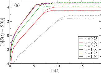
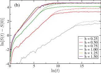
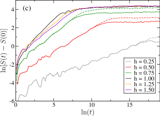
Figure 1: Dynamical entropy after a quench from $h_{0}=0$ to various values of $h$ at the aperiodicity parameters (a) $r=0.75$, (b) $r=0.5$ and (c) $r=0.25$. The solid lines are the results for $L=F_{16}=987$, and the dashed lines (only at $h=0.25$, $h=0.5$ and $h=0.75$) correspond to the data for $L=F_{17}=1597$. The ”noise” (irregular variation) present on the curves in the small $t$ regime is due to such low-energy excitations, which are related to local properties of the quasiperiodic chain and are independent of the chain lengths.

For a chain of total length $F_{n}$ with periodic boundary conditions, we have calculated the entanglement entropy $S_{\ell}$ between a block of length $\ell=F_{n-2}$ and its environment which has a length of $F_{n-1}$. Various values of $0<r<1$ for the inhomogeneity amplitude were considered. We start our numerical calculations from the fully ordered state with $h_{0}=0$ to a state with $h>0$ both in the ordered and in the disordered phases, as well as at the critical point. The numerical results for ${\cal S}_{\ell}(t)-{\cal S}_{\ell}(0)$ are shown in figure 1. For all cases considered, $S_{\ell}(t)$ exhibits two time-regimes: in the late-time regime, the entropy is saturated to an $L$ dependent value, similar to the behavior for the homogeneous chain; in the early-time regime, it increases with time as a power-law form:

$${\cal S}(t)\sim t^{\sigma}\;,$$ (16)

with some exponent $\sigma<1$. Our numerical results show that the exponent $\sigma$ depends on the value of the transverse field in the final state, while it does not vary (significantly) with the initial $h_{0}$. The values of $\sigma$ for $r=0.25$, $0.5$ and $0.75$ are plotted in figure 6; for all cases considered, $\sigma$ reaches its maximum at the critical point $h=1$, and the increase with $h$ in the ordered phase ($h<1$) is much faster than the decrease in the disordered phase ($h>1$). Furthermore, we have found that the exponent $\sigma$ decreases with stronger inhomogeneity, that is with smaller value of $r$.

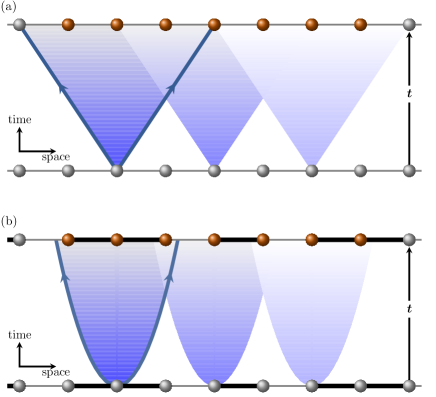
Figure 2: Schematic illustration of the light cones of quasiparticles for a homogeneous quantum Ising chain (a) and for a chain with an aperiodic modulation of the couplings (the thin/thick lines between sites represent weak/strong couplings according to a Fibonacci sequence) (b). The quasiparticle excitations emitted at time $t=0$ move ballistically in the homogeneous lattice, while their motion is anomalous diffusive with $x\sim t^{D}$ ($D<1$) in the quasiperiodic lattice. Pairs of quasiparticles moving to the left or right from a given point are entangled; they will contribute to the entanglement entropy between a region $A$ (the region with orange sites) and the rest of the chain, region $B$, if they arrive simultaneously in $A$ and $B$.

The power-law time-dependence of the entanglement entropy in (16) is a new feature of the quasiperiodic system: the increase in entropy is slower than in the homogeneous chain, but faster than in a random chain. This behavior can be explained in terms of quasiparticles that are emitted at time $t=0$, and subsequently move classically by anomalous diffusion which has a power-law relationship between displacement and time, $x\sim t^{D}$, with a diffusion exponent $0<D<1$. We note that in a homogeneous chain pairs of quasiparticles that contribute to the entanglement entropy move ballistically (i.e. $x\sim t$) rather than moving by diffusion, which results in the linear growth of the entanglement entropy with time [33] (figure 2). The dynamics of the quasiparticles in our quasiperiodic lattice will be studied in more detail in section 4.3.

4.2 Local magnetization

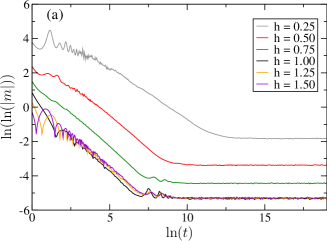
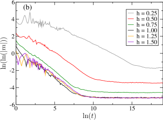
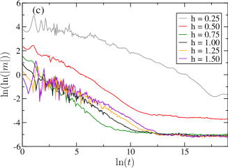
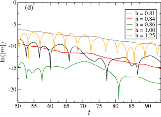
Figure 3: Double logarithm of the bulk magnetization as a function of the logarithm of the time. During the quench the transverse field is changed from $h_{0}=0$ to different values of $h$ at the aperiodicity parameter $r=0.75$ (panel (a)), $r=0.5$ (panel (b)), $r=0.25$ (panel (c)). The length of the chain is $L=F_{17}=1597$ and the magnetization is considered at site $l=F_{16}=987$. In panel (d) $\ln|m_{\mathrm{b}}(t)|$ is shown as a function of $t$ in the window $50<t<100$ for different values of $h$ at $r=0.5$. The oscillations in $\ln|m_{\mathrm{b}}(t)|$ (i.e. in the prefactor $A(t)$) occur when $h$ is larger than a certain value $h^{*}$ (here $h^{*}\approx 0.85$), and the oscillations disappear for $h<h^{*}$; the dynamical phase transition described in the main text occurs at $h^{*}$.

The local magnetization, $m_{l}(t)$, is calculated for open chains of length $L=F_{n}$. Generally $m_{l}(t)$ has a monotonic position dependence: $m_{l_{1}}(t)>m_{l_{2}}(t)$ for $l_{1}<l_{2}<L/2$. We measured the magnetization at site $l=F_{n-1}$, which is considered as the bulk magnetization and denoted by $m_{\mathrm{b}}(t)$. We have also studied the behavior of the surface magnetization, $m_{1}(t)$, for which some exact results are obtained.

We study the asymptotic behavior of the surface magnetization (given in (61)) for large $t$ after a quench. If the quench is performed to the ordered phase, $h<1$, the lowest excitation energy is $\epsilon_{1}=0$ (i.e. $\cos(\epsilon_{1}t)=1$); consequently $P_{1,2k-1}(t)$ in (35) has a time independent part. This results in a non-oscillating contribution to the surface magnetization: $\overline{m_{1}}=\lim_{t\to\infty}\int_{0}^{t}m_{1}(t^{\prime}){\rm d}t^{\prime}$ which is given by:

$$\overline{m_{1}}=\Phi_{1}(1)\sum_{j=1}^{L}\Phi_{1}(j)\Phi_{1}^{(0)}(j)\;,$$ (17)

and defines its stationary value. Recall that $\Phi_{1}(1)=m_{1}(h,t=0)$, i.e. it is equal to the equilibrium surface magnetization [90, 91], which is finite for $h<1$, and zero in the disordered phase. Similarly, $\Phi_{1}^{(0)}(1)>0$ for $h_{0}<1$ and zero otherwise. From this it follows that the stationary nonequilibrium surface magnetization is $\overline{m_{1}}>0$, if both $h<1$ and $h_{0}<1$. Otherwise the stationary surface magnetization vanishes. If the quench starts from the fully ordered initial state $h_{0}=0$, then $\Phi^{(0)}_{1}(j)=\delta_{1,j}$ and $\overline{m_{1}}=\Phi_{1}^{2}(1)$; thus we obtain the simple relation:

$$\overline{m_{1}}(h)=[m_{1}(h,t=0)]^{2}\;,$$ (18)

which is generally valid between the stationary value of the nonequilibrium surface magnetization and its equilibrium value. From (18) it follows that the critical exponent $\beta_{\mathrm{s}}^{\mathrm{ne}}$ for the nonequilibrium surface magnetization and the critical exponent $\beta_{\mathrm{s}}$ for the equilibrium surface magnetization are related as: $\beta_{\mathrm{s}}^{\mathrm{ne}}=2\beta_{\mathrm{s}}$. According to (18) and [92], for the Fibonacci chain close to the critical point $h\to h_{c}=1$, we have $\overline{m_{1}}(h)\sim 1-h^{2}=(h_{c}-h)(h_{c}+h)\sim h_{c}-h$, thus $\beta_{s}^{\mathrm{ne}}=1$.

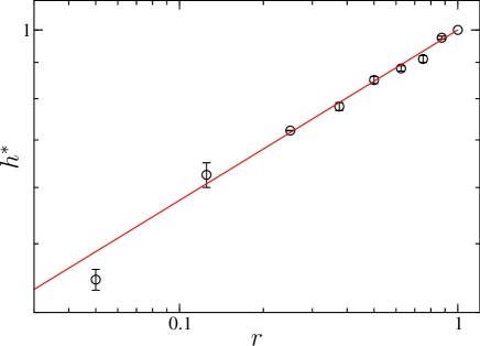
Figure 4: Position of the dynamical critical point for different values of the aperiodicity parameter in a double-logarithmic plot. The straight line has a slope $\alpha=0.24$.

We numerically calculated the time-dependence of the bulk magnetization after a quench from the fully ordered initial state, $h_{0}=0$, to different values of $h$. For fixed values of the inhomogeneity $r=0.25,\,0.5,\,0.75$, the results for the double logarithm of $|m_{\mathrm{b}}(t)|$ are shown in figure 3(a-c) as functions of $\ln t$. In each case one can observe a linear dependence, which implies that the magnetization has asymptotically a stretched exponential time dependence:

$$m_{\mathrm{b}}(t)\sim A(t)\exp\left(-Ct^{\mu}\right)\;.$$ (19)

which corresponds to equation (14) for a homogeneous system, with $\mu=1$. Before analyzing the decay exponent $\mu$, we first study the behavior of the prefactor $A(t)$. Like in a homogeneous chain as discussed in section 3.2, there is a dynamical phase transition between a non-oscillating phase for $h<h^{*}(r)$, where the order-parameter ${\cal O}$ defined in (15) is zero, and an oscillating phase for $h>h^{*}(r)$, where ${\cal O}>0$. In the oscillating phase, the characteristic time-scale defined as the period time, $t_{\rm per}(h,r)$, becomes divergent as $h\to h^{*}(r)^{+}$. An example for this behavior is illustrated in figure 3, panel (d), in which $\ln|m_{\mathrm{b}}(t)|$ as a function of $t$ is shown in the window $50<t<100$ for different values of $h$ at $r=0.5$; as seen in this figure, the curves for $h=0.86,1.0$ and $1.25$ oscillate, whereas the oscillations vanish for $h=0.81$ and $h=0.84$. We identify the dynamical phase transition point as $h^{*}=0.850(5)$. In this quasiperiodic model the dynamical phase transition does not coincide with the equilibrium phase transition, since $h^{*}(r)<1$ for $r<1$. Estimates of $h^{*}(r)$ versus $r$ are shown in figure 4; the data are well approximated by a power-law $h^{*}(r)\sim r^{\alpha}$ with $\alpha=0.24(3)$ [93].

The exponent $\mu$ describing the decay of the local magnetization dependents both on $h$ and $r$; by contrast, it does not vary significantly with $h_{0}$, at least for $h_{0}<h$. Our results for the critical exponents $\mu=\mu(h,r)$ are plotted in figure 6 for $r=0.75,~{}0.5$ and $0.25$ as functions of $h$. The exponent $\mu$ reaches its maximum at the dynamical phase transition point $h^{*}(r)$.

4.3 Interpretation by wave packet dynamics

As is known from previous studies on the homogeneous chain, dynamical features of the entanglement entropy and the local magnetization can be well described by the dynamics of quasiparticles. To understand the dynamical properties of the quasiparticles emitted after a quantum quench in the quasiperiodic lattice, we regard the quasiparticles as wave packets and study their dynamics using a method that has been applied to studies of transport properties of quasicrystals [44, 94].

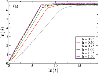
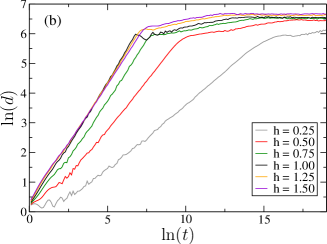
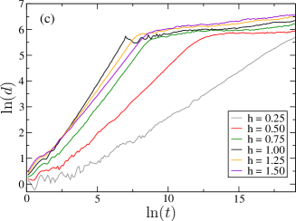
Figure 5: Time-dependent width of the wave-packet at different values of $h$ for $r=0.75$ (panel (a)), $r=0.5$ (panel (b)), $r=0.25$ (panel (c)).

We construct a wave packet connecting sites $k$ and $l$ at time $t$ in the form:

$$W_{l,k}(t)= \frac{1}{2} \sum_{q}\biggl{\{}\cos(\epsilon_{q}t)\bigl{[}\Phi_{q}(l)\Phi_{q}(k)+\Psi_{q}(l)\Psi_{q}(k)\bigr{]}\biggr{.}$$ (20)

$$- \biggl{.}\imath\sin(\epsilon_{q}t)\bigl{[}\Phi_{q}(l)\Psi_{q}(k)+\Phi_{q}(k)\Psi_{q}(l)\bigr{]}\biggr{\}},$$

which is localized at $t=0$ since $W_{l,k}(0)=\delta_{l,k}$ (cf. equation (8)). For a Hamiltonian with eigenfunctions $\phi_{q}(l)$ and eigenvalues $\epsilon_{q}$, a wave packet can be obtained by: $W_{l,k}(t)=\sum_{q}\cos(\epsilon_{q}t)\phi_{q}(l)\phi_{q}(k)$, which corresponds to the first term in (20). We note that (20) is just a linear combination of the four time-dependent factors in (35), which describe the time dependence of the fermion operators. The width of the wave packet starting from site $k$ after time $t$ is given by:

$$d(k,t)=\left[\sum_{l}(k-l)^{2}|W_{l,k}(t)|^{2}\right]^{\frac{1}{2}}\;.$$ (21)

The spreading of a wave packet in a perfect crystal with absolutely continuous energy spectrum is known to be ballistic, i.e. the width increases linearly in time. A heuristic argument is the following [95]: the energy scale $\Delta\epsilon$ defined by the typical variation of the energy levels is proportional to the inverse of the time that a wave packet needs to spread over the chain. In the case of the absolutely continuous spectrum, we have $\Delta\epsilon\sim L^{-1}$, which gives $d\sim L\sim t$. In case of a singular continuous spectrum as for our quasiperiodic lattice, there are many energy scales $\Delta\epsilon\sim L^{-1/\alpha}$ with a number of exponents $\alpha$. One then expects that for large $t$ the wave packet in the infinite quasiperiodic lattice shows anomalous diffusion in the form $d(k,t)\sim t^{D(k)}$ with a diffusion exponent $D(k)$, which may depend on the starting position. Here we determine the value of $D(k)$ numerically.

After a global quench, quasiparticles are emitted everywhere in lattices, therefore $d(k,t)$ should be averaged over different initial positions,

$$d(t)=\overline{d(k,t)}\sim t^{D}\;.$$ (22)

In our numerical calculations chains of length $L=F_{17}=1597$ with periodic boundary conditions were considered. First we have confirmed that the wave packet constructed in our method moves ballistically in the homogeneous chain (with $r=1$), corresponding to $D=1$. In the quasiperiodic chains the motion is indeed anomalous diffusive with $D<1$, which is seen in figure 5 where the average widths of the wave packet are presented as functions of time in a log-log plot for various values of $h$ and $r=0.75,~{}0.5$ and $0.25$. The diffusion exponent $D$ for given $h$ and $r$ corresponds to the slope of the linear part of the function.

The variation of $D$ with $h$ at a fixed $r$ is shown in figure 6, compared with the exponent $\sigma$ for the entanglement entropy and the exponent $\mu$ for the local magnetization. Here one can observe that the agreement between these three exponents is very good for $h<h^{*}(r)$, i.e. in the non-oscillating phase, but the exponent for the magnetization deviates in the oscillating phase ($h>h^{*}(r)$). The discrepancy in the oscillating phase implies that the semiclassical picture breaks down in the oscillating phase, where the quasiparticles cannot be well described by the moving kinks in the magnetization.

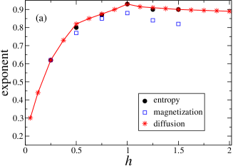
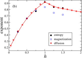
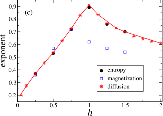
Figure 6: Scaling exponents calculated from the time-dependence of the width of the wave-packet, from the entanglement entropy and from the magnetization at different values of $h$ for $r=0.75$ (panel (a)), $r=0.5$ (panel (b)), $r=0.25$ (panel (c)). The full lines connecting the diffusion exponents are guides for the eye.

5 Discussion

In this paper we have studied the nonequilibrium dynamics of quasiperiodic quantum Ising chains after a global quench. In a quench process, the complete spectrum of the Hamiltonian is relevant for the the time evolution of various observables. For the quasiperiodic quantum Ising chain the spectrum is in a very special form, which is given by a Cantor set of zero Lebesgue measure, i.e. purely singular continuous. We have calculated numerically two quantities: the dynamical entanglement entropy and the relaxation of the local magnetization. The entanglement entropy is found to increase in time as a power-law (see (16)), whereas the bulk magnetization decays in a stretched exponential way (see (19)). Both behaviors can be explained in a quasiparticle picture, in which the quasiparticles move by anomalous diffusion in the quasiperiodic lattice. The diffusion exponent has been calculated by a wave packet approach, and good agreement has been found with the exponents that we obtained for the entropy and for the magnetization. We note that the anomalous dynamics found in the global quench process is similar to the transport properties of quasicrystals.

Relaxation of the bulk magnetization is found to present a nonequilibrium dynamical phase transition. The non-oscillating phase, in which the magnetization is always positive, and the oscillating phase, in which the sign of the magnetization varies periodically in time, is separated by a dynamical phase transition point, at which the time-scale of oscillations diverges. This singularity point, due to collective dynamical effects, is different from the equilibrium critical point.

A similar nonequilibrium dynamical behavior is expected to hold for other quasiperiodic or aperiodic quantum models as long as the spectrum of the Hamiltonian is also purely singular continuous; there is a large class of such models, for example the Thue-Morse quantum Ising chain. If, however the spectrum of the Hamiltonian of the model is in a different type, such as the Harper potential which has extended or localized states, the nonequilibrium dynamics is expected to be different than the case we consider in this paper.

Appendix A Free-fermionic calculation of the time-dependent local magnetization

To calculate the local magnetization in (12), we need to first calculate the time dependence of the spin operator $\sigma_{l}^{x}(t)$ at site $l$ in the Heisenberg picture. We introduce at each site two Majorana fermion operators, $\check{a}_{2l-1}$ and $\check{a}_{2l}$, defined in terms of the free fermion operators $\eta_{k}^{\dagger}$ and $\eta_{k}$ (given in (7)) as

$$\check{a}_{2l-1} = \sum_{k=1}^{L}\Phi_{k}(l)(\eta_{k}^{\dagger}+\eta_{k})\;,$$

$$\check{a}_{2l} = -\imath\sum_{k=1}^{L}\Psi_{k}(l)(\eta_{k}^{\dagger}-\eta_{k})\;.$$ (23)

These satisfy the commutation relations:

$$\check{a}_{l}^{{\dagger}}=\check{a}_{l},\quad\{\check{a}_{l},\check{a}_{k}\}=2\delta_{l,k}\;.$$ (24)

The spin operators are then expressed in terms of the Majorana operators as:

$$\sigma_{l}^{x} = \;\imath^{l-1}\prod_{j=1}^{2l-1}\check{a}_{j}\;,$$ (25)

and the local magnetization in (12) is then given as the expectation value of product of fermion operators with respect to the ground state:

$$m_{l}(t)=(\imath)^{l-1}\langle\mathit{\Psi}^{(0)}_{0}|\prod_{j=1}^{2l-1}\check{a}_{j}(t)\eta_{1}|\mathit{\Psi}^{(0)}_{0}\rangle\;,$$ (26)

where we have used: $|\mathit{\Psi}^{(0)}_{1}\rangle=\eta_{1}|\mathit{\Psi}^{(0)}_{0}\rangle$. The expression in (26) - according to Wick’s theorem - can be expressed as a sum of products of two-operator expectation values. This can be written in a compact form of a Pfaffian, which in turn can be evaluated as the square root of the determinant of an antisymmetric matrix:

$$m_{l}(t)=(-\imath)^{l-1}\left|\begin{array}[]{cccc}\langle\check{a}_{1}(t)\check{a}_{2}(t)\rangle&\langle\check{a}_{1}(t)\check{a}_{3}(t)\rangle&\cdots\quad\langle\check{a}_{1}(t)\check{a}_{2l-1}(t_{1})\rangle&\langle\check{a}_{1}(t)\eta_{1}\rangle\\ &\langle\check{a}_{2}(t)\check{a}_{3}(t)\rangle&\cdots\quad\langle\check{a}_{2}(t)\check{a}_{2l-1}(t)\rangle&\langle\check{a}_{2}(t)\eta_{1}\rangle\\ &\ddots&&\vdots\cr&&\langle\check{a}_{2l-2}(t)\check{a}_{2l-1}(t)\rangle&\langle\check{a}_{2l-2}(t)\eta_{1}\rangle\\ &&&\langle\check{a}_{2l-1}(t)\eta_{1}\rangle\end{array}\right|$$ (32)

$$=\pm\left[{\rm det}\,C_{ij}\right]^{1/2}\;,$$ (33)

where $C_{ij}$ is the antisymmetric matrix $C_{ij}=-C_{ji}$, with the elements of the Pfaffian (33) above the diagonal. (Here and in the following we use the short-hand notation: $\langle\dots\rangle=\langle\mathit{\Psi}^{(0)}_{0}|\dots|\mathit{\Psi}^{(0)}_{0}\rangle$.)

Below we describe how the time evolution of the spin operator $\sigma_{l}^{x}$ follows from the time dependence of the Majorana fermion operators. Inserting $\eta_{k}^{\dagger}(t)=e^{\imath t\epsilon_{k}}\eta_{k}^{\dagger}$ and $\eta_{k}(t)=e^{-\imath t\epsilon_{k}}\eta_{k}$ into (23) one obtains

$$\check{a}_{m}(t)=\sum_{n=1}^{2L}P_{m,n}(t)\check{a}_{n}\;,$$ (34)

with

$$P_{2l-1,2k-1} = \sum_{q}\cos(\epsilon_{q}t)\Phi_{q}(l)\Phi_{q}(k),$$

$$P_{2l-1,2k} = -\sum_{q}\sin(\epsilon_{q}t)\Phi_{q}(l)\Psi_{q}(k)\;,$$

$$P_{2l,2k-1} = \sum_{q}\sin(\epsilon_{q}t)\Phi_{q}(k)\Psi_{q}(l)\;,$$

$$P_{2l,2k} = \sum_{q}\cos(\epsilon_{q}t)\Psi_{q}(l)\Psi_{q}(k)\;.$$ (35)

The two-operator expectation values are given by:

$$\langle\check{a}_{m}(t)\check{a}_{n}(t)\rangle=\sum_{k_{1},k_{2}}P_{m,k_{1}}(t)P_{n,k_{2}}(t)\langle\check{a}_{k_{1}}\check{a}_{k_{2}}\rangle\;.$$ (36)

The equilibrium correlations in the initial state with a transverse field $h_{0}$ are:

$$\langle\check{a}_{2m-1}\check{a}_{2n-1}\rangle=\langle\check{a}_{2m}\check{a}_{2n}\rangle = \delta_{m,n},$$ (37)

$$\langle\check{a}_{2m-1}\check{a}_{2n}\rangle=-\langle\check{a}_{2m}\check{a}_{2n-1}\rangle = \imath G^{(0)}_{n,m}\;,$$ (38)

where the static correlation matrix $G^{(0)}_{m,n}$ is given by:

$$G^{(0)}_{m,n}=-\sum_{q}\Psi_{q}^{(0)}(m)\Phi_{q}^{(0)}(n)\;,$$ (39)

where $\Psi_{q}^{(0)}(m)$ and $\Phi_{q}^{(0)}(n)$ are the components of the eigenvectors in (10), calculated for the initial Hamiltonian. Then (36) can be written in the form:

$$\langle\check{a}_{m}(t)\check{a}_{n}(t)\rangle=\delta_{m,n}+\imath\Gamma_{m,n}(t)\;,$$ (40)

with

$$\Gamma_{2l-1,2m-1} = \sum_{k_{1},k_{2}}\left[G^{(0)}_{k_{2},k_{1}}P_{2l-1,2k_{1}-1}P_{2m-1,2k_{2}}\right.$$ (41)

$$- \left.G^{(0)}_{k_{1},k_{2}}P_{2l-1,2k_{1}}P_{2m-1,2k_{2}-1}\right]$$ (42)

$$\Gamma_{2l-1,2m} = \sum_{k_{1},k_{2}}\left[G^{(0)}_{k_{2},k_{1}}P_{2l-1,2k_{1}-1}P_{2m,2k_{2}}\right.$$ (43)

$$- \left.G^{(0)}_{k_{1},k_{2}}P_{2l-1,2k_{1}}P_{2m,2k_{2}-1}\right]$$ (44)

$$\Gamma_{2l,2m-1} = -\sum_{k_{1},k_{2}}\left[G^{(0)}_{k_{2},k_{1}}P_{2l,2k_{2}}P_{2m-1,2k_{1}-1}\right.$$ (45)

$$- \left.G^{(0)}_{k_{1},k_{2}}P_{2l,2k_{2}-1}P_{2m-1,2k_{1}}\right]$$ (46)

$$\Gamma_{2l,2m} = \sum_{k_{1},k_{2}}\left[G^{(0)}_{k_{2},k_{1}}P_{2l,2k_{1}-1}P_{2m,2k_{2}}\right.$$ (47)

$$- \left.G^{(0)}_{k_{1},k_{2}}P_{2l,2k_{1}}P_{2m,2k_{2}-1}\right]\,.$$ (48)

In (33) there are also the contractions:

$$\Pi_{m} = \langle\mathit{\Psi}^{(0)}_{0}|\check{a}_{m}(t)\eta_{1}|\mathit{\Psi}^{(0)}_{0}\rangle$$ (49)

$$= \sum_{n}P_{m,n}\langle\mathit{\Psi}^{(0)}_{0}|\check{a}_{n}\eta_{1}|\mathit{\Psi}^{(0)}_{0}\rangle$$ (50)

where

$$\langle\mathit{\Psi}^{(0)}_{0}|\check{a}_{2l-1}\eta_{1}|\mathit{\Psi}^{(0)}_{0}\rangle = \Phi_{1}^{(0)}(l)$$ (51)

$$\langle\mathit{\Psi}^{(0)}_{0}|\check{a}_{2l}\eta_{1}|\mathit{\Psi}^{(0)}_{0}\rangle = \imath\Psi_{1}^{(0)}(l)\;.$$ (52)

Thus finally the square of the local magnetization is given by the determinant:

$$m_{l}^{2}(t)=\left|\begin{array}[]{cccccc}0&\Gamma_{1,2}&\Gamma_{1,3}&\cdots\quad\Gamma_{1,2l-1}&\Pi_{1}\cr-\Gamma_{1,2}&0&\Gamma_{2,3}&\cdots\quad\Gamma_{2,2l-1}&\Pi_{2}\cr-\Gamma_{1,3}&-\Gamma_{2,3}&0&\cdots\quad\Gamma_{3,2l-1}&\Pi_{3}\cr&&&\ddots&\vdots\cr-\Gamma_{1,2l-1}&\cdots&&0&\Pi_{2l-1}\cr-\Pi_{1}&\cdots&&-\Pi_{2l-1}&0\end{array}\right|$$ (59)

As a special case, the surface magnetization is expressed as:

$$m_{1}(t)=\Pi_{1} = \sum_{j=1}^{L}P_{1,2j-1}(t)\Phi_{1}^{(0)}(j)$$ (60)

$$- \imath\sum_{j=1}^{L}P_{1,2j}(t)\Psi_{1}^{(0)}(j)\;.$$ (61)

References

References

- [1] Greiner M, Mandel O, Hänsch T W, and Bloch I 2002 Nature 419 51
- [2] Paredes B et al. 2004 Nature 429 277
- [3] Kinoshita T, Wenger T and Weiss D S 2004 Science 305 1125
- [4] Sadler L E, Higbie J M, Leslie S R, Vengalattore M, and Stamper-Kurn D M 2006 Nature 443 312
- [5] Lamacraf A 2006 Phys. Rev. Lett. 98 160404
- [6] Kinoshita T, Wenger T and Weiss D S 2006 Nature 440 900
- [7] Hofferberth S, Lesanovsky I, Fischer B, Schumm T, and Schmiedmayer J 2007 Nature 449 324
- [8] Trotzky S, Chen Y-A, Flesch A, McCulloch I P, Schollwöck U Eisert J, and Bloch I 2012 Nature Phys. 8 325
- [9] Cheneau M, Barmettler P, Poletti D, Endres M, Schauss P, Fukuhara T, Gross C, Bloch I, Kollath C and Kuhr S 2012 Nature 481 484
- [10] Gring M, Kuhnert M, Langen T, Kitagawa T, Rauer B, Schreitl M, Mazets I, Smith D A, Demler E and Schmiedmayer J 2012 Science 337 1318
- [11] Polkovnikov A, Sengupta K, Silva A, and Vengalattore M 2011 Rev. Mod. Phys. 83 863
- [12] Rigol M, Dunjko V, Yurovsky V and Olshanii M 2007 Phys. Rev. Lett. 98 50405 Rigol M, Dunjko V and Olshanii M 2008 Nature 452 854
- [13] Calabrese P and Cardy J 2006 Phys. Rev. Lett. 96 136801
- [14] Calabrese P and Cardy J 2007 J. Stat. Mech. P06008
- [15] Cazalilla M A 2006 Phys. Rev. Lett. 97 156403Iucci A and Cazalilla M A 2010 New J. Phys. 12 055019Iucci A and Cazalilla M A 2009 Phys. Rev. A 80 063619
- [16] Manmana S R, Wessel S, Noack R M and Muramatsu A 2007 Phys. Rev. Lett. 98 210405
- [17] Cramer M, Dawson C M, Eisert J and Osborne T J 2008 Phys. Rev. Lett. 100 030602Cramer M and Eisert J 2010 New J. Phys. 12 055020Cramer M, Flesch A, McCulloch I A, Schollwöck U and Eisert J 2008 Phys. Rev. Lett. 101 063001Flesch A, Cramer M, McCulloch I P, Schollwöck U and Eisert J 2008 Phys. Rev. A 78 033608
- [18] Barthel T and Schollwöck U 2008 Phys. Rev. Lett. 100 100601
- [19] Kollar M and Eckstein M 2008 Phys. Rev. A 78 013626
- [20] Sotiriadis S, Calabrese P and Cardy J 2009 EPL 87 20002
- [21] Roux G 2009 Phys. Rev. A 79 021608Roux G 2010 Phys. Rev. A 81 053604
- [22] Sotiriadis S, Fioretto D and Mussardo G 2012 J. Stat. Mech. P02017Fioretto D and Mussardo G 2010 New J. Phys. 12 055015Brandino G P, De Luca A, Konik R M, and Mussardo G 2012 Phys. Rev. B 85 214435
- [23] Kollath C, Läuchli A and Altman E 2007 Phys. Rev. Lett. 98 180601Biroli G, Kollath C and Läuchli A 2010 Phys. Rev. Lett. 105 250401
- [24] Banuls M C, Cirac J I, and Hastings M B 2011 Phys. Rev. Lett. 106 050405
- [25] Gogolin C, Müller M P and Eisert J 2011 Phys. Rev. Lett. 106 040401
- [26] Rigol M and Fitzpatrick M 2011 Phys. Rev. A 84 033640
- [27] Caneva T, Canovi E, Rossini D, Santoro G E and Silva A 2011 J. Stat. Mech. P07015
- [28] Cazalilla M A, Iucci A, and Chung M-C 2012 Phys. Rev. E 85 011133
- [29] Rigol M and Srednicki M 2012 Phys. Rev. Lett. 108 110601
- [30] Santos L F, Polkovnikov A and Rigol M 2011 Phys. Rev. Lett. 107 040601
- [31] Grisins P and Mazets I E 2011 Phys. Rev. A 84 053635
- [32] Canovi E, Rossini D, Fazio R, Santoro G E and Silva A 2011 Phys. Rev. B 83 094431
- [33] Calabrese P and Cardy J 2005 J. Stat. Mech. P04010
- [34] Rieger H and Iglói F 2011 Phys. Rev. B 84 165117
- [35] De Chiara G, Montangero S, Calabrese P, Fazio R 2006 J. Stat. Mech., L03001
- [36] Iglói F, Szatmári Z and Lin Y-C 2012 Phys. Rev. B 85 094417
- [37] Levine G C, Bantegui M J, Burg J A 2012 arXiv:1201.3933
- [38] Bardarson J H, Pollmann F and Moore J E 2012 Phys. Rev. Lett. 109 017202
- [39] Vosk R and Altman E 2012 arXiv:1205.0026
- [40] Shechtman D, Blech I, Gratias D and Cahn J W 1984 Phys. Rev. Lett. 53 1951
- [41] Dubois J-M 2005 Useful Quasicrystals (World Scientific, Singapore London)
- [42] Penrose R 1974 Bull. Inst. Math. Appl. 10 266
- [43] Stadnik Z M 1999 Physical Properties of Quasicrystals (Springer, Berlin Heidelberg New York)
- [44] Roche S, Trambly de Laissardiére G and Mayou D 1997 J. Math. Phys. 38 1794Mayou D, Berger C, Cyrot-Lackmann F, Klein T and Lanco P 1993 Phys. Rev. Lett. 70 3915
- [45] Roati G, D’Errico C, Fallani L, Fattori M, Fort C, Zaccanti M, Modugno G, Modugno M and Inguscio M 2008 Nature 453 895
- [46] Deissler B, Lucioni E, Modugno M, Roati G, Tanzi L, Zaccanti M, Inguscio M and Modugno G 2011 New J. Phys. 13 023020
- [47] Harper P G 1955 Proc. Phys. Soc. A 68 874
- [48] Aubry S and André G 1980 Ann. Isr. Phys. Soc. 3 133
- [49] Modugno M 2009 New J. Phys. 11 033023
- [50] Gramsch C and Rigol M 2012 arXiv:1206.3570
- [51] Barouch E, McCoy B and Dresden M 1970 Phys. Rev. A 2 1075Barouch E and McCoy B 1971 Phys. Rev. A 3 786Barouch E and McCoy B 1971 Phys. Rev. A 3 2137
- [52] Iglói F and Rieger H 2000 Phys. Rev. Lett. 85 3233
- [53] Sengupta K, Powell S and Sachdev S 2004 Phys. Rev. A 69 053616
- [54] Fagotti M and Calabrese P 2008 Phys. Rev. A 78 010306
- [55] Silva A 2008 Phys. Rev. Lett. 101 120603Gambassi A and Silva A 2011 arXiv:1106.2671
- [56] Rossini D, Silva A, Mussardo G and Santoro G 2009 Phys. Rev. Lett. 102 127204Rossini D, Suzuki S, Mussardo G, Santoro G E and Silva A 2010 Phys. Rev. B 82 144302
- [57] Campos Venuti L and Zanardi P 2010 Phys. Rev. A 81 022113Campos Venuti L, Jacobson N T, Santra S and Zanardi P 2011 Phys. Rev. Lett. 107 010403
- [58] Iglói F and Rieger H 2011 Phys. Rev. Lett. 106 035701
- [59] Divakaran U, Iglói F, Rieger H 2011 J. Stat. Mech. P10027
- [60] Foini L, Cugliandolo L F and Gambassi A 2011 Phys. Rev. B 84 212404Foini L, Cugliandolo L F and Gambassi A 2012 J. Stat. Mech. P09011
- [61] Calabrese P, Essler F H L and Fagotti M 2011 Phys. Rev. Lett. 106 227203
- [62] Schuricht D and Essler F H L 2012 J. Stat. Mech. P04017
- [63] Calabrese P, Essler F H L and Fagotti M 2012 J. Stat. Mech. P07016
- [64] Calabrese P, Essler F H L and Fagotti M 2012 J. Stat. Mech. P07022
- [65] Blaß B, Rieger H and Iglói F 2012 EPL 99 30004
- [66] Essler F H L, Evangelisti S, Fagotti M 2012 arXiv:1208.1961
- [67] Iglói F 1988 J. Phys. A 21 L911Doria M M and Satija I I 1988 Phys. Rev. Lett. 60 444Ceccatto H A 1989 Phys. Rev. Lett. 62 203Ceccatto H A 1989 Z. Phys. B 75 253Benza G V 1989 Europhys. Lett. 8 321Henkel M and Patkós A 1992 J. Phys. A 25 5223
- [68] Turban L, Iglói F and Berche B 1994 Phys. Rev. B 49 12695
- [69] Iglói F and Turban L 1996 Phys. Rev. Lett. 77 1206
- [70] Iglói F, Turban L, Karevski D and Szalma F 1997 Phys. Rev. B, 56 11031
- [71] Hermisson J, Grimm U and Baake M 1997 J. Phys. A: Math. Gen. 30 7315
- [72] Hermisson J 2000 J. Phys. A: Math. Gen. 33 57
- [73] Iglói F, Juhász R and Zimborás Z 2007 Europhys. Lett. 79 37001
- [74] Jordan P and Wigner E 1928 Z. Phys. 47 631
- [75] Lieb E, Schultz T and Mattis D 1961 Ann. Phys. (N.Y.) 16 407Pfeuty P 1970 Ann. Phys. (Paris) 57 79
- [76] Pfeuty P 1979 Phys. Lett. 72A 245
- [77] Onsager L 1944 Phys. Rev. 65 117
- [78] Luck J M 1993 Europhys. Lett. 24 359Iglói F 1993 J. Phys. A 26 L703
- [79] Sütő A 1995 Beyond Quasicrystals, ed F Axel and D Gratias (Springer-Verlag & Les Editions de Physique) p. 481
- [80] Damanik D 2000 J. Math. Anal. App., 249 393Damanik D and Gorodetski A 2011 Comm. Math. Phys. 205 221
- [81] Yessen W N 2012 arXiv:1203.2221
- [82] Iglói F, Szatmári Z and Lin Y-C 2009 Phys. Rev. B 80 024405
- [83] Fagotti M and Calabrese P 2008 Phys. Rev. A 78 010306(R)
- [84] Eisler V, Iglói F and Peschel I 2009 J. Stat. Mech. P02011
- [85] Fisher D S 1995 Phys. Rev. B 51 6411
- [86] For a review, see: Iglói F and Monthus C 2005 Physics Reports 412 277
- [87] Yang C N 1952 Phys. Rev. 85 808
- [88] Sachdev A and Young A P 1997 Phys. Rev. Lett. 78 2220
- [89] Iglói F, unpublished.
- [90] Peschel I 1984 Phys. Rev. B 30 6783
- [91] Iglói F and Rieger H 1998 Phys. Rev. B 57 4238
- [92] Iglói F, Rieger H and Turban L 1999 Phys. Rev. E 59 1465
- [93] No oscillation of the magnetization is expected if all sites are “locally” in the ferromagnetic phase. This condition is satisfied for a weakly coupled site having one strong () and one weak () bond, and if , which means . The numerical results in figure 4 indicate that the critical value, coincides with .
- [94] Poon S J 1992 Adv. Phys. 41 303Yuan H Q, Grimm U, Repetowicz P and Schreiber M 2000 Phys. Rev. B 62 15569Schulz-Baldes H and Bellissard J 1998 Rev. Math. Phys. 10 1Huckestein B and Schweitzer L 1994 Phys. Rev. Lett. 72 713Thiem S and Schreiber M 2012 Phys. Rev. B 85 224205
- [95] Thouless D J 1977 Phys. Rev. Lett. 39 1167Piéchon F 1996 Phys. Rev. Lett. 76 4372