On-Fiber Optomechanical Cavity

Abstract

A fully on-fiber optomechanical cavity is fabricated by patterning a suspended metallic mirror on the tip of an optical fiber. Optically induced self-excited oscillations of the suspended mirror are experimentally demonstrated. We discuss the feasibility of employing on-fiber optomechanical cavities for sensing applications. A theoretical analysis evaluates the sensitivity of the proposed sensor, which is assumed to operate in the region of self-excited oscillations, and the results are compared with the experimental data. Moreover, the sensitivity that is obtained in the region of self-excited oscillations is theoretically compared with the sensitivity that is achievable when forced oscillations are driven by applying an oscillatory external force.

Optomechanical cavities, which are formed by coupling an optical cavity with a mechanical resonator, are currently a subject of intense study.Marquardt_0905_0566 ; girvin_Trend ; Kippenberg_1172 Such systems may allow experimental study of the crossover from classical to quantum mechanics (see Ref. Meystre_1210_3619 for a recent review). In addition, optomechanical cavities can be employed in optical communications Wu_et_al_06 and in other photonics applications.Stokes_et_al_90 ; Hossein-Zadeh&Vahala_10 When the finesse of the optical cavity that is employed for constructing the optomechanical cavity is sufficiently high, the coupling to the mechanical resonator that serves as a vibrating mirror is typically dominated by the effect of radiation pressure.Kippenberg_1172 On the other hand, bolometric effects can contribute to the optomechanical coupling when optical absorption by the vibrating mirror is significant.Metzger_1002 ; Jourdan_et_al_08 ; Metzger_133903 ; Marino&Marin_10 In general, bolometric effects play an important role in relatively large mirrors, in which the thermal relaxation rate is comparable to the mechanical resonance frequency. Aubin_et_al_04 ; Marquardt_103901 ; Paternostro_et_al_06 ; Liberato_et_al_10 Phenomena such as mode cooling and self-excited oscillations Hane_179 ; Kim_1454225 ; Aubin_1018 ; Carmon_223902 ; Marquardt_103901 ; Corbitt_021802 ; Carmon_123901 ; Metzger_133903 have been shown in systems in which bolometric effects are dominant. Metzger_133903 ; Metzger_1002 ; Aubin_et_al_04 ; Jourdan_et_al_08 ; Zaitsev_046605 ; Zaitsev_1589

In this paper we study a novel configuration, in which an optomechanical cavity is constructed using a single mode optical fiber. In this configuration the vibrating mirror is fabricated on the tip of an optical fiber. Additional static reflector is introduced in the fiber, so that optomechanical cavity is formed. We experimentally demonstrate that self-excited oscillations of the vibrating mirror can be induced by injecting a monochromatic laser light into the fiber. This effect is attributed to the bolometric optomechanical coupling between the optical mode and the mechanical resonator.

The ability to optically induce self-excited oscillations can be exploited for operating an on-fiber optomechanical cavity as a sensor. Such a device can sense physical parameters (e.g. absorbed mass, heating by external radiation, acceleration, etc.) that affect the resonance frequency of the suspended mirror. The simplicity of fabrication and operation, the small size and robustness of such a device and the unneeded actuator coupling and circuitry might be beneficial for future sensor applications. Further we present the on-fiber optomechanical cavity showing self-excited oscillations, give a theoretical estimate of its sensitivity and compare it with the measured performance.

The optomechanical cavity seen in Fig. 1 was fabricated on the tip of a single mode fused silica optical fiber (Corning SMF-28 operating at wavelength $\lambda\approx 1550\operatorname{nm}$). The processing started from thermal evaporation of chromium and then gold layers with thicknesses of $10$ and $200\operatorname{nm}$ respectively, on a flat polished tip of a fiber, held in a zirconia ferrule. The evaporated layers were directly patterned by a focused ion beam to the desired mirror shape ($20\operatorname{\mu m}$ wide doubly clamped beam). Finally, the gold mirror was released by etching the underlying silica in 7% HF acid (90 $\operatorname{min}$ etch time), while the beam remained supported by the zirconia ferrule. The precise alignment of the micro-mechanical mirror and fiber core that was achieved in this process allowed robust and simple operation of the fiber-tip devices without a need of any post fabrication positioning.

The static mirror of the optomechanical cavity was provided by a fiber Bragg grating (FBG) mirror of high reflectivity (the FBG stopband of $0.4\operatorname{nm}$ FWHM was centered at $\lambda$) that is made using the phase mask technique (see Fig. 1). The length of the optical cavity was $l\approx 10\operatorname{mm}$ providing a free spectral range $\Delta\lambda=\lambda^{2}/2n_{\mathrm{eff}}l\approx 80$ pm (where $n_{\mathrm{eff}}$ $=1.47$ is the effective refraction index for SMF-28); five resonant wavelengths were located within the range of the FBG stopband.

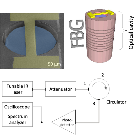
Figure 1: The experimental set-up. On- fiber optomechanical cavity excited by a tunable laser. The reflected light intensity is measured and analyzed. Inset: electron micrograph of a suspended micromechanical mirror (color code: blue-silica fiber, yellow - gold mirror, gray-zirconia ferrule),view is tilted by 52^o .

Monochromatic light was injected into the fiber bearing the cavity on its tip from a laser source with adjustable output wavelength (between $1525$ and $1575\operatorname{nm}$) and power level (up to $20\operatorname{mW}$). The source was connected through an optical circulator, that allowed the reflected light intensity to be measured by a fast responding photodetector. The detected signal was analyzed by an oscilloscope and a spectrum analyzer. The experiments were performed with samples in vacuum (at residual pressure below $10$ mPa) thermally anchored to a cold finger with temperature adjustable between $4$ to $300$ $\operatorname{K}$. The resonance frequency of the suspended mirror oscillations, $\omega_{0}$ was estimated by the frequency of thermal oscillations measured at input laser power well below the self-excited oscillations threshold.

In Fig. 2 we present the spectral power density of the reflected light intensity as a function of optical excitation wavelength. The sharp spectral peaks that appear just below the mechanical resonance frequency $\omega_{0}$ (which is marked by a dashed line in Fig. 2) indicate the appearance of the self-excited oscillations of the vibrating mirror. These oscillations are ”turned on” when the incoming laser power exceeds a threshold value and the laser wavelength is adjusted to the regions of high (positive) slope of the cavity reflectance spectrum (Fig. 2, solid curve). The sign of the reflectivity slope suggests that the beam is buckled.Yuvaraj_1207_0947

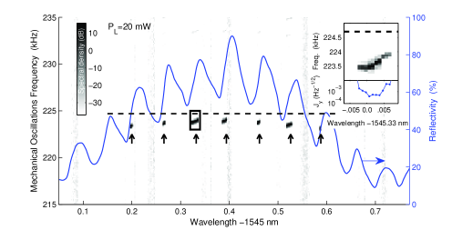
Figure 2: The self-excited oscillations visible as sharp peaks (dark gray regions on colormap, marked by arrows) in reflected power spectrum are obtained at optical excitation wavelengths corresponding to positive slope of the sample reflectivity (shown by a solid curve). The self-excited oscillations frequency is slightly below the estimated mechanical resonance frequency, indicated by a dashed line. Zoom-in to a self-excited oscillations peak (marked by a rectangle) and estimation of sensitivity factor $J_{\mathrm{y}}$ are shown in the inset.

To estimate the sensitivity of such a sensor that is based on optomechanical cavity the phase noise of the self-excited oscillations is theoretically evaluated below, and the results are compared with experimental data. In general, the resonant detection with a mechanical resonator is a widely employed technique in a variety of applications.Larsen_121901 ; Ilic_et_al_04 ; Cleland_235 ; Pandey_et_al_10 A detector belonging to this class typically consists of a mechanical resonator, which is characterized by an angular resonance frequency $\Omega$ and characteristic damping rate $\Gamma$. Detection is achieved by coupling the measured physical parameter of interest, denoted as $p$, to the resonator in such a way that $\Omega$ becomes effectively $p$ dependent, i.e. $\Omega=\Omega\left(p\right)$. The sensitivity of the detection scheme that is employed for monitoring the parameter of interest $p$ can be characterized by the minimum detectable change in $p$, denoted as $\delta p$. For small changes, $\delta p$ is related to the normalized minimum detectable change in the frequency $\sigma_{\mathrm{y}}=\delta\Omega/\Omega$ by the relation $\delta p=\left|\partial\Omega/\partial p\right|^{-1}\Omega\sigma_{\mathrm{y}}$. The dimensionless parameter $\sigma_{\mathrm{y}}$, in turn, typically depends on the noise in the system and on the averaging time $\tau$ that is employed for the measurement.

A commonly employed detection scheme is based on externally driving the resonator with a monochromatic force at a frequency close to the resonance frequency and employing homodyne detection for monitoring the response. For this detection scheme the normalized minimum detectable change in the frequency $\sigma_{\mathrm{y}}$ is found to be given by Cleland_2758

$$\sigma_{\mathrm{y}}=\left(\frac{2\Gamma k_{\mathrm{B}}T_{\mathrm{eff}}}{U_{0}\Omega^{2}\tau}\right)^{1/2}\ ,$$ (1)

where $k_{\mathrm{B}}$ is the Boltzmann’s constant, $T_{\mathrm{eff}}$ is the noise effective temperature and $U_{0}$ is the energy stored in the externally driven resonator in steady state. Note that Eq. (1) is derived by assuming that the response of the resonator is linear and by assuming the classical limit, i.e. $k_{\mathrm{B}}T_{\mathrm{eff}}\gg\hbar\Omega$. The generalization of Eq. (1) for the case of nonlinear response is discussed in Ref. Buks_026217 .

In some cases applying external driving is technically difficult. For example, for the case of the on-fiber optomechanical cavity, external driving that is based on capacitive coupling requires electrical wiring to the device that is located on the tip of the fiber as well as a closely positioned reference electrode. On the other hand, these difficulties can be avoided by exploiting the back-action effects resulting from optomechanical coupling, which can be used for optically inducing self-excited oscillations of the mechanical resonator.Zaitsev_046605 This method, which significantly simplifies the operation since no oscillatory external drive is needed, can be employed as an alternative resonant detection scheme.

In the limit of small displacement, the dynamics of the system can be approximately described using a single evolution equation.Zaitsev_1589 The theoretical model that is used to derive the evolution equation is briefly described below. Note that some optomechanical effects that were taken into account in the theoretical modeling Zaitsev_1589 were found experimentally to have a negligible effect on the dynamics Zaitsev_046605 (e.g. the effect of radiation pressure). In what follows such effects are disregarded.

The micromechanical mirror in the optical cavity is treated as a mechanical resonator with a single degree of freedom $x$ having mass $m$ and damping rate $\gamma_{0}$ (when it is decoupled from the optical cavity). It is assumed that the angular resonance frequency $\omega_{m}$ of the mechanical resonator depends on the temperature $T$ of the suspended mirror. For small deviation of $T$ from the base temperature $T_{0}$ (i.e. the temperature of the supporting substrate) $\omega_{m}$ is taken to be given by $\omega_{m}=\omega_{0}-\beta\left(T-T_{0}\right)$, where $\beta$ is a constant. Furthermore, to model the effect of thermal deformation Metzger_133903 it is assumed that a temperature dependent force given by $F_{\text{{th}}}=\theta\left(T-T_{0}\right)$, where $\theta$ is a constant, acts on the mechanical resonator. The mechanical oscillator’s equation of motion is given by $\ddot{x}+2\gamma_{0}\dot{x}+\omega_{m}^{2}x=F_{\text{{th}}}$, where an overdot denotes differentiation with respect to time.

The time evolution of the effective temperature $T$ is governed by the thermal balance equation $\dot{T}=\kappa\left(T_{0}-T\right)+\eta P_{\mathrm{L}}I\left(x\right)$, where $\eta$ is the heating coefficient due to optical absorption, $\kappa$ is the thermal rate, $P_{\mathrm{L}}$ is the injected laser power and $P_{\mathrm{L}}I\left(x\right)$ is the intra-cavity optical power incident on the suspended mirror, which depends on the mechanical displacement $x$ (i.e. on the length of the optical cavity) due to the effect of optical interference. For small $x$ the expansion $I\left(x\right)\simeq I_{0}+I_{0}^{\prime}x+\left(1/2\right)I_{0}^{\prime\prime}x^{2}$ is employed, where a prime denotes differentiation with respect to the displacement $x$. This model neglects the mechanical nonlinearities of the resonator, i.e. it is assumed that nonlinear behavior exclusively originates from bolometric optomechanical coupling.

The displacement $x\left(t\right)$ can be expressed in terms of the complex amplitude $A$ as $x\left(t\right)=x_{0}+2\operatorname{Re}A$, where $x_{0}$, which is given by $x_{0}=\eta\theta P_{\mathrm{L}}I_{0}/\kappa\omega_{0}^{2}$, is the optically-induced static displacement. For small displacement the evolution equation for the complex amplitude $A$ is found to be given by Zaitsev_1589

$$\dot{A}+\left(\Gamma_{\mathrm{eff}}+i\Omega_{\mathrm{eff}}\right)A=\xi\left(t\right)\;,$$ (2)

where both the effective resonance frequency $\Omega_{\mathrm{eff}}$ and the effective damping rate $\Gamma_{\mathrm{eff}}$ are real even functions of $\left|A\right|$. To second order in $\left|A\right|$ they are given by

$$\Gamma_{\mathrm{eff}} =\gamma_{0}+\frac{\eta\theta P_{\mathrm{L}}}{2\omega_{0}^{2}}I_{0}^{\prime}+\frac{\eta\beta P_{\mathrm{L}}}{4\omega_{0}}I_{0}^{\prime\prime}\left|A\right|^{2}\;,$$ (3)

$$\Omega_{\mathrm{eff}} =\omega_{0}-\frac{\eta\beta P_{\mathrm{L}}}{\kappa}I_{0}-\frac{\eta\beta P_{\mathrm{L}}}{\kappa}I_{0}^{\prime\prime}\left|A\right|^{2}\;.$$ (4)

The above expressions for $\Gamma_{\mathrm{eff}}$ and $\Omega_{\mathrm{eff}}$ are obtained by making the following assumptions $\beta x_{0}\ll\theta/2\omega_{0}$, $\theta\kappa^{2}\ll\beta\omega_{0}^{3}\lambda$ and $\kappa\ll\omega_{0}$, which typically hold experimentally.Zaitsev_046605 The fluctuating term Risken_Fokker-Planck $\xi\left(t\right)=\xi_{x}\left(t\right)+i\xi_{y}\left(t\right)$, where both $\xi_{x}$ and $\xi_{y}$ are real, represents white noise and the following is assumed to hold $\left\langle\xi_{x}\left(t_{1}\right)\xi_{x}\left(t_{2}\right)\right\rangle=\left\langle\xi_{y}\left(t_{1}\right)\xi_{y}\left(t_{2}\right)\right\rangle=2\Theta\delta\left(t_{1}-t_{2}\right)$ and $\left\langle\xi_{x}\left(t_{1}\right)\xi_{y}\left(t_{2}\right)\right\rangle=0$ where $\Theta=\gamma_{0}k_{\mathrm{B}}T_{\mathrm{eff}}/4m\omega_{0}^{2}$ and where $T_{\mathrm{eff}}$ is the effective noise temperature.

In cylindrical coordinates $A$ is expressed as $A=A_{r}e^{iA_{\theta}}$, where $A_{r}=\left|A\right|$ and where $A_{\theta}$ is real.Hempstead_350 The equations of motion for $A_{r}$ and for $A_{\theta}$ are given by [see Eq. (2)] $\dot{A}_{r}+A_{r}\Gamma_{\mathrm{eff}}=\xi_{r}\left(t\right)$ and $\dot{A}_{\theta}+\Omega_{\mathrm{eff}}\left(A_{r}\right)=\left(1/A_{r}\right)\xi_{\theta}\left(t\right)$, where the fluctuating terms satisfy the following relations $\left\langle\xi_{r}\left(t_{1}\right)\xi_{r}\left(t_{2}\right)\right\rangle=\left\langle\xi_{\theta}\left(t_{1}\right)\xi_{\theta}\left(t_{2}\right)\right\rangle=2\Theta\delta\left(t_{1}-t_{2}\right)$ and $\left\langle\xi_{r}\left(t_{1}\right)\xi_{\theta}\left(t_{2}\right)\right\rangle=0$.

By introducing the notation $\Gamma_{0}=\gamma_{0}+\eta\theta P_{\mathrm{L}}I_{0}^{\prime}/2\omega_{0}^{2}$ and $\Gamma_{2}=\eta\beta P_{\mathrm{L}}I_{0}^{\prime\prime}/4\omega_{0}$ one can express the effective damping rate $\Gamma_{\mathrm{eff}}$ as [see Eq. (3)] $\Gamma_{\mathrm{eff}}=\Gamma_{0}+\Gamma_{2}A_{r}^{2}$. Consider the case where $I_{0}^{\prime}<0$ and where $I_{0}^{\prime\prime}>0$. For such a case a supercritical Hopf bifurcation occurs when $\Gamma_{0}$ vanishes, i.e. for a critical value of the laser power given by $P_{\mathrm{LC}}=-2\omega_{0}^{2}\gamma_{0}/\eta\theta I_{0}^{\prime}$. The self-excited oscillations emerge above the threshold, i.e. when $\Gamma_{0}$ becomes negative, with steady state value of $A_{r}$ (when noise is disregarded) given by $r_{0}=\sqrt{-\Gamma_{0}/\Gamma_{2}}$, . In terms of the laser power $r_{0}$ can be expressed as

$$r_{0}=\lambda\sqrt{-\frac{2\theta}{\beta\omega_{0}\lambda}\frac{I_{0}^{\prime}}{\lambda I_{0}^{\prime\prime}}\frac{\Delta P_{\mathrm{L}}}{P_{\mathrm{L}}}}\;,$$ (5)

where $\Delta P_{\mathrm{L}}=P_{\mathrm{L}}-P_{\mathrm{LC}}$.

Using the notation $A_{r}=r_{0}+\rho$ one finds to lowest nonvanishing order in $\rho$ that $A_{r}\Gamma_{\mathrm{eff}}=-2\Gamma_{0}\rho+O\left(\rho^{2}\right)$. Moreover $\Omega_{\mathrm{eff}}=\Omega_{\mathrm{H}}+\zeta\rho+O\left(\rho^{2}\right)$, where $\Omega_{\mathrm{H}}=\Omega_{\mathrm{eff}}\left(r_{0}\right)$ and where $\zeta=\mathrm{d}\Omega_{\mathrm{eff}}/\mathrm{d}A_{r}$ at the point $r_{0}$. To lowest nonvanishing order in $\rho$ the equations of motion for $A_{r}$ and $A_{\theta}$ become $\dot{\rho}-2\Gamma_{0}\rho=\xi_{r}\left(t\right)$ and $\dot{\phi}+\zeta\rho=r_{0}^{-1}\xi_{\theta}\left(t\right)$, where $\phi=A_{\theta}+\Omega_{\mathrm{H}}t$. In steady state (i.e. in the limit $t\rightarrow\infty$) the solution for $\rho$ reads $\rho\left(t\right)=\int_{0}^{t}e^{2\Gamma_{0}\left(t-t_{1}\right)}\xi_{r}\left(t_{1}\right)\;\mathrm{d}t_{1}$. The correlation function of $\rho\left(t\right)$ is found to be given by $\left\langle\rho\left(t_{1}\right)\rho\left(t_{2}\right)\right\rangle=-\left(\Theta/2\Gamma_{0}\right)e^{2\Gamma_{0}\left|t_{1}-t_{2}\right|}$, and thus the correlation function of $\dot{\phi}$ is given by

$$\left\langle\dot{\phi}\left(t_{1}\right)\dot{\phi}\left(t_{2}\right)\right\rangle=\Theta\left[\frac{\zeta^{2}e^{2\Gamma_{0}\left|t_{1}-t_{2}\right|}}{2\left|\Gamma_{0}\right|}+2\frac{\Gamma_{2}}{\left|\Gamma_{0}\right|}\delta\left(t_{1}-t_{2}\right)\right]\;.$$ (6)

With the help of the above result together with Wiener-Khinchine theorem one finds that power spectrum $S_{\dot{\phi}}\left(\omega\right)$ of $\dot{\phi}$ is given by

$$S_{\dot{\phi}}\left(\omega\right)=\frac{1}{\pi}\frac{\Theta\zeta^{2}}{4\Gamma_{0}^{2}+\omega^{2}}+\frac{\Theta\Gamma_{2}}{\pi\left|\Gamma_{0}\right|}\;.$$ (7)

The signal $y\left(t\right)\equiv\dot{\phi}/\Omega_{\mathrm{H}}$ represents the normalized deviation of the momentary angular frequency $\Omega+\dot{\phi}$ from its average value. The average value of $y\left(t\right)$ is estimated by monitoring the signal $y\left(t\right)$ in a time interval $\tau$, i.e. $\hat{y}\left(\tau\right)=\tau^{-1}\int_{-\tau/2}^{\tau/2}\mathrm{d}t\;y\left(t\right)$. In the limit of steady state, i.e. when $\tau\gg 1/\left|\Gamma_{0}\right|$, the variance of the estimator $\hat{y}\left(\tau\right)$ is given by $\sigma_{\mathrm{y}}^{2}\left(\tau\right)=2\pi S_{\mathrm{y}}\left(0\right)/\tau$, thus $\sigma_{\mathrm{y}}^{2}\left(\tau\right)=\left(2\Theta/\Omega_{\mathrm{H}}^{2}r_{0}^{2}\tau\right)\left(1+\zeta^{2}/4\left|\Gamma_{0}\right|\Gamma_{2}\right)$. Note that due to the fact that in the present case $S_{\dot{\phi}}\left(\omega\right)$ remains finite in the limit $\omega\rightarrow 0$ the above defined variance $\sigma_{\mathrm{y}}^{2}\left(\tau\right)$ is identical to the Allan variance.Allan_221 ; Cutler_136 ; Walls_162 With the help of Eq. (4) one finds that $\zeta^{2}/4\left|\Gamma_{0}\right|\Gamma_{2}=\left(4\omega_{0}/\kappa\right)^{2}$. The assumption that $\kappa\ll\omega_{0}$ Zaitsev_046605 leads to

$$\sigma_{\mathrm{y}}\left(\tau\right)=\frac{4\omega_{0}}{\kappa}\left(\frac{2\gamma_{0}k_{\mathrm{B}}T_{\mathrm{eff}}}{U_{0}\omega_{0}^{2}\tau}\right)^{1/2}\;,$$ (8)

where $U_{0}=4m\Omega_{\mathrm{H}}^{2}r_{0}^{2}$ is the energy stored in the self-excited resonator in steady state close to the threshold. The comparison with Eq. (1) indicates that $\sigma_{\mathrm{y}}\left(\tau\right)$ for the case of optically induced self-excited oscillations is roughly $4\omega_{0}/\kappa$ times larger compared with the case of external drive for the same values of $U_{0}$ and $T_{\mathrm{eff}}$.

In general, the sensitivity factor $J_{\mathrm{p}}$ of a physical parameter $p$ is given by $J_{\mathrm{p}}=\left|\partial\log\Omega/\partial p\right|^{-1}J_{\mathrm{y}}$, where $J_{\mathrm{y}}=\sigma_{\mathrm{y}}\tau^{1/2}$ represents the sensitivity factor of the parameter $y$. The factor $J_{\mathrm{y}}$ as function of $P_{\mathrm{L}}$ is experimentally measured using an on-fiber optomechanical cavity device, in which the mechanical mirror covers almost the entire fiber cross section. Self-excited oscillation as a function of input power has been observed above a threshold value of $P_{\mathrm{LC}}=8.7\operatorname{mW}$ [see Fig. 3 (a)]. To experimentally determine the factor $J_{\mathrm{y}}$ the reflected optical power is recorded over a time period of $2\operatorname{ms}$ using an oscilloscope. The standard deviation $\sigma_{\mathrm{y}}$, which is found by the zero-crossing technique Cutler_136 , allows evaluation of the factor $J_{\mathrm{y}}=\sigma_{\mathrm{y}}\tau^{1/2}$. The frequency of self-excited oscillations $\Omega_{\mathrm{H}}/2\pi$ and the sensitivity factor $J_{\mathrm{y}}$ are plotted vs. laser power $P_{\mathrm{L}}$ in panels (a) and (b) respectively of Fig. 3. The red solid line in panel (a) represents a theoretical fit that is based on Eq. (4) and the one in panel (b) is based on Eqs. (5) and (8). The experimental parameters that have been employed in both cases are listed in the figure caption. Similar measurements of the factor $J_{\mathrm{y}}$ with other on-fiber devices (e.g. results shown in the inset of Fig. 2) as well as with devices that were made on a wafer have yielded values having the same order of magnitude [as in the data seen in Fig. 3(b)].

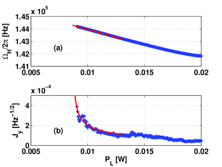
Figure 3: The frequency of self-excited oscillations $\Omega_{\mathrm{H}}/2\pi$ [panel (a)] and the sensitivity factor $J_{\mathrm{y}}$ [panel (b)] vs. laser power $P_{\mathrm{L}}$. The blue cross marks represent experimental data, the red solid lines represent a theoretical fit that is based on the following experimental parameters: $\kappa=22\times 10^{3}\operatorname{Hz}$, $m=30\times 10^{-12}\operatorname{kg}$, $\lambda=1.55\operatorname{\mu m}$, $T_{\mathrm{eff}}=300\operatorname{K}$, $\Omega/\Gamma=10^{3}$, $\left|I_{0}^{\prime}\right|/\lambda I_{0}^{\prime\prime}=0.8$, $\beta=10^{4}\operatorname{s}^{-1}\operatorname{K}^{-1}$, $\theta=1.6\times 10^{-3}\operatorname{N}\operatorname{kg}^{-1}\operatorname{K}^{-1}$ and $\eta=3.5\times 10^{6}\operatorname{K}\operatorname{J}^{-1}$.

In summary, optically induced self-excited oscillations of suspended mirror fabricated on tip of an optical fiber were experimentally demonstrated. Based on previously developed model of bolometrically coupled optomechanical cavity we estimated the sensitivity of a detector exploiting the self-excited oscillations effect. The fabrication and operation simplicity of self-excited oscillating optomechanical detectors in many cases compensates the possible degradation in sensitivity compared to traditional externally actuated resonator.

This work was supported by the German Israel Foundation under Grant No. 1-2038.1114.07, the Israel Science Foundation under Grant No. 1380021, the Deborah Foundation, the Mitchel Foundation, the Israel Ministry of Science, the Russell Berrie Nanotechnology Institute, the European STREP QNEMS Project, MAGNET Metro 450 consortium and MAFAT. The work of IB was supported by a Zeff Fellowship.

References

- (1) T. J. Kippenberg and K. J. Vahala, “Cavity optomechanics: Back-action at the mesoscale,” Science, vol. 321, no. 5893, pp. 1172–1176, Aug 2008.
- (2) F. Marquardt and S.M. Girvin, “Optomechanics (a brief review),” arXiv preprint arXiv:0905.0566, 2009.
- (3) S.M. Girvin, “Trend: Optomechanics,” Physics, vol. 2, pp. 40, 2009.
- (4) P. Meystre, “A short walk through quantum optomechanics,” arXiv:1210.3619, 2012.
- (5) M. C. Wu, O. Solgaard, and J. E. Ford, “Optical MEMS for lightwave communication,” J. Lightwave Technol., vol. 24, no. 12, pp. 4433–4454, Dec 2006.
- (6) N. A. D. Stokes, R. M. A. Fatah, and S. Venkatesh, “Self-excitation in fibre-optic microresonator sensors,” Sens. Actuators, A, vol. 21, pp. 369–372, Feb 1990.
- (7) M. Hossein-Zadeh and K. J. Vahala, “An optomechanical oscillator on a silicon chip,” IEEE J. Sel. Top. Quantum Electron., vol. 16, no. 1, pp. 276–287, Jan 2010.
- (8) C. H. Metzger and K.Karrai, “Cavity cooling of a microlever,” Nature, vol. 432, pp. 1002–1005, 2004.
- (9) G. Jourdan, F. Comin, and J. Chevrier, “Mechanical mode dependence of bolometric backaction in an atomic force microscopy microlever,” Phys. Rev. Lett., vol. 101, pp. 133904, Sep 2008.
- (10) C. Metzger, M. Ludwig, C. Neuenhahn, A. Ortlieb, I. Favero, K. Karrai, and F. Marquardt, “Self-induced oscillations in an optomechanical system driven by bolometric backaction,” Phys. Rev. Lett., vol. 101, pp. 133903, Sep 2008.
- (11) F. Marino and F. Marin, “Chaotically spiking attractors in suspended mirror optical cavities,” arXiv:1006.3509, Jun 2010.
- (12) K. Aubin, M. Zalalutdinov, T. Alan, R.B. Reichenbach, R. Rand, A. Zehnder, J. Parpia, and H. Craighead, “Limit cycle oscillations in CW laser-driven NEMS,” J. Microelectromech. Syst., vol. 13, pp. 1018 – 1026, Dec 2004.
- (13) F. Marquardt, J. G. E. Harris, and S. M. Girvin, ,” Phys. Rev. Lett., vol. 96, pp. 103901, 2006.
- (14) M. Paternostro, S. Gigan, M. S. Kim, F. Blaser, H. R. Böhm, and M. Aspelmeyer, “Reconstructing the dynamics of a movable mirror in a detuned optical cavity,” New J. Phys., vol. 8, pp. 107, Jun 2006.
- (15) S. D. Liberato, N. Lambert, and F. Nori, “Quantum limit of photothermal cooling,” arXiv:1011.6295, Nov 2010.
- (16) K. Hane and K. Suzuki, “Self-excited vibration of a self-supporting thin film caused by laser irradiation,” Sensors and Actuators A: Physical, vol. 51, pp. 179–182, 1996.
- (17) K. Kim and S. Lee, “Self-oscillation mode induced in an atomic force microscope cantilever,” J. Appl. Phys., vol. 91, pp. 4715–4719, 2002.
- (18) K. Aubin, M. Zalalutdinov, T. Alan, R.B. Reichenbach, R. Rand, A. Zehnder, J. Parpia, and H. Craighead, “Limit cycle oscillations in CW laser-driven NEMS,” J. MEMS, vol. 13, pp. 1018–1026, 2004.
- (19) T. Carmon, H. Rokhsari, L. Yang, T. J. Kippenberg, and K. J. Vahala, ,” Phys. Rev. Lett., vol. 94, pp. 223902, 2005.
- (20) T. Corbitt, D. Ottaway, E. Innerhofer, J. Pelc, and N. Mavalvala, ,” Phys. Rev. A, vol. 74, pp. 21802, 2006.
- (21) T. Carmon and K. J. Vahala, ,” Phys. Rev. Lett., vol. 98, pp. 123901, 2007.
- (22) S. Zaitsev, A. K. Pandey, O. Shtempluck, and E. Buks, “Forced and self-excited oscillations of optomechanical cavity,” Phys. Rev. E 84, vol. 84, pp. 046605, 2011.
- (23) S. Zaitsev, O. Gottlieb, and E. Buks, “Nonlinear dynamics of a microelectromechanical mirror in an optical resonance cavity,” Nonlinear Dyn., vol. 69, pp. 1589–1610, 2012.
- (24) D. Yuvaraj, M. B. Kadam, Oleg Shtempluck, and Eyal Buks, “Optomechanical cavity with a buckled mirror,” arXiv: 1207.0947, 2012, JMEMS, in press.
- (25) T. Larsen, S. Schmid, L. Gr nberg, A. O. Niskanen, J. Hassel, S. Dohn, and A. Boisen, “Ultrasensitive string-based temperature sensors,” Appl. Phys. Lett., vol. 98, pp. 121901, 2011.
- (26) B. Ilic, H. G. Craighead, S. Krylov, W. Senaratne, and C. Ober, “Attogram detection using nanoelectromechanical oscillators,” J. Appl. Phys., vol. 95, Apr 2004.
- (27) A. N. Cleland, “Thermomechanical noise limits on parametric sensing with nanomechanical resonators,” New J. Phys., vol. 7, pp. 235, 2005.
- (28) A. K. Pandey, O. Gottlieb, O. Shtempluck, and E. Buks, “Performance of an AuPd micromechanical resonator as a temperature sensor,” Appl. Phys. Lett., vol. 96, pp. 203105, 2010.
- (29) A. N. Cleland and M. L. Roukes, “Noise processes in nanomechanical resonators,” J. Appl. Phys., vol. 92, no. 5, pp. 2758–2769, Sep 2002.
- (30) Eyal Buks, Stav Zaitsev, Eran Segev, Baleegh Abdo, and M. P. Blencowe, “Displacement detection with a vibrating RF SQUID: Beating the standard linear limit,” Phys. Rev. E, vol. 76, pp. 26217, 2007.
- (31) Hannes Risken, The Fokker-Planck Equation: Methods of Solution and Applications, Springer, 1996.
- (32) Robert D. Hempstead and Melvin Lax, “Classical noise. vi. noise in self-sustained oscillators near threshold,” Phys. Rev., vol. 161, pp. 350–366, Sep 1967.
- (33) David W. Allan, “Statistics of atomic frequency standards,” Proc. IEEE, vol. 54, pp. 221–230, 1966.
- (34) L. S. Cutler and C. L. Searle, “,some aspects of the theory andmeasurement of frequency fluctuations in frequency standards,” ,Proc. IEEE, vol. 54, pp. 136–154, 1966.
- (35) F.L. Walls and D.W. Allan, “Measurements of frequency stability,” Proc. IEEE, vol. 74, pp. 162–168, 1986.