The Pilot-Wave Perspective on Quantum Scattering and Tunneling

Abstract

The de Broglie - Bohm “pilot-wave” theory replaces the paradoxical wave-particle duality of ordinary quantum theory with a more mundane and literal kind of duality: each individual photon or electron comprises a quantum wave (evolving in accordance with the usual quantum mechanical wave equation) and a particle that, under the influence of the wave, traces out a definite trajectory. The definite particle trajectory allows the theory to account for the results of experiments without the usual recourse to additional dynamical axioms about measurements. Instead one need simply assume that particle detectors click when particles arrive at them. This alternative understanding of quantum phenomena is illustrated here for two elementary textbook examples of one-dimensional scattering and tunneling. We introduce a novel approach to reconciling standard textbook calculations (made using unphysical plane-wave states) with the need to treat such phenomena in terms of normalizable wave packets. This allows for a simple but illuminating analysis of the pilot-wave theory’s particle trajectories and an explicit demonstration of the equivalence of the pilot-wave theory predictions with those of ordinary quantum theory.

I Introduction

The pilot-wave version of quantum theory was originated in the 1920s by Louis de Broglie, re-discovered and developed in 1952 by David Bohm, and championed in more recent decades especially by John Stewart Bell. dbb Usually described as a “hidden variable” theory, the pilot-wave account of quantum phenomena supplements the usual description of quantum systems – in terms of wave functions – with definite particle positions that obey a deterministic evolution law. This can be understood as the simplest possible account of “wave-particle duality”: individual particles (electrons, photons, etc.) manage to behave sometimes like waves and sometimes like particles because each one is literally both. In, for example, an interference experiment involving a single electron, the final outcome will be a function of the position of the particle at the end of the experiment. (In short, detectors “click” when particles hit them.) But the trajectory of the particle is not at all classical; it is instead determined by the structure of the associated quantum wave which guides or “pilots” the particle.

The main virtue of the theory, however, is not its deterministic character, but rather the fact that it eliminates the need for ordinary quantum theory’s “unprofessionally vague and ambiguous” measurement axioms. bellqft Instead, in the pilot-wave picture, measurements are just ordinary physical processes, obeying the same fundamental dynamical laws as other processes. In particular, nothing like the infamous “collapse postulate” – and the associated Copenhagen notion that measurement outcomes are registered in some separately-postulated classical world – are needed. The pointers, for example, on laboratory measuring devices will end up pointing in definite directions because they are made of particles – and particles, in the pilot-wave picture, always have definite positions.

In the “minimalist” presentation of the pilot-wave theory (advocated especially by J.S. Bell), the guiding wave is simply the usual quantum mechanical wave function $\Psi$ obeying the usual Schrödinger equation:

$$i\hbar\frac{\partial\Psi}{\partial t}=-\frac{\hbar^{2}}{2m}\frac{\partial^{2}\Psi}{\partial x^{2}}+V(x)\Psi.$$ (1)

The particle position $X(t)$ evolves according to

$$\frac{dX}{dt}=\left.\frac{j}{\rho}\right|_{x=X(t)}$$ (2)

where

$$j=\frac{\hbar}{2mi}(\Psi^{*}\frac{\partial}{\partial x}\Psi-\Psi\frac{\partial}{\partial x}\Psi^{*})$$ (3)

(the usual quantum probability current) and $\rho=|\Psi|^{2}$ (the usual quantum probability density) satisfy the continuity equation

$$\frac{\partial\rho}{\partial t}+\frac{\partial j}{\partial x}=0.$$ (4)

Here we consider the simplest possible case of a single spinless particle moving in one dimension. The generalizations for motion in 3D and particles with spin are trivial: $\partial/\partial x$ and $j$ become vectors, and the wave function becomes a multi-component spinor obeying the appropriate wave equation. For a system of $N$ particles, labelled $i\in\left\{1,...,N\right\}$, the generalization is also straightforward, though it should be noted that $\Psi$ – and consequently also $\vec{j}_{i}$ and $\rho$ – are in this case functions on the system’s configuration space. The velocity of particle $i$ at time $t$ is given by the ratio $\vec{j}_{i}/\rho$ evaluated at the complete instantaneous configuration; thus in general the velocity of each particle depends on the instantaneous positions of all other particles. The theory is thus explicitly non-local. Bell, upon noticing this surprising feature of the pilot-wave theory, was famously led to prove that such non-locality is a necessary feature of any theory sharing the empirical predictions of ordinary quantum theory. belltheorem

Although the fundamental dynamical laws in the pilot-wave picture are deterministic, the theory exactly reproduces the usual stochastic predictions of ordinary quantum mechanics. This arises from the assumption that, although the initial wave function can be controlled by the usual experimental state-preparation techniques, the initial particle position is random. In particular, for an ensemble of identically-prepared quantum systems having $t=0$ wave function $\Psi(x,0)$, it is assumed that the initial particle positions $X(0)$ are distributed according to

$$P[X(0)\!=\!x]=|\Psi(x,0)|^{2}.$$ (5)

This is called the “quantum equilibrium hypothesis” or QEH. It is then a purely mathematical consequence of the already-postulated dynamical laws for $\Psi$ and $X$ that the particle positions will be $|\Psi|^{2}$ distributed for all times:

$$P[X(t)\!=\!x]=|\Psi(x,t)|^{2},$$ (6)

a property that has been dubbed the “equivariance” of the $|\Psi|^{2}$ probability distribution. dgz To see this, one need simply note that the probability distribution $P$ for an ensemble of particles moving in a velocity field $v(x,t)$ will evolve according to

$$\frac{\partial P}{\partial t}+\frac{\partial}{\partial x}(vP)=0.$$ (7)

Since $j$ and $\rho$ satisfy the continuity equation, it is then immediately clear that, for $v=j/\rho$, $P=\rho$ is a solution.

Properly understood, the QEH can actually be derived from the basic dynamical laws of the theory, much as the expectation that complex systems should typically be found in thermal equilibrium can be derived in classical statistical mechanics. dgz2 For our purposes, though, it will be sufficient to simply take the QEH as an additional assumption, from which it follows that the pilot-wave theory will make the same predictions as ordinary quantum theory for any experiment in which the outcome is registered by the final position of the particle. That the pilot-wave theory makes the same predictions as ordinary QM for arbitrary measurements then follows from the fact that, at the end of the day, such measurement outcomes are also registered in the position of something: think, for example, of the flash on a screen somewhere behind a Stern-Gerlach magnet, the position of a pointer on a laboratory measuring device, or the distribution of ink droplets in Physical Review. bellqft

In the present paper, our goal is to illustrate all of these ideas by showing in concrete detail how the pilot-wave theory deals with some standard introductory textbook examples of one-dimensional quantum scattering and tunneling. This alternative perspective should be of interest to students and teachers of this material, since it provides an illuminating and compelling intuitive picture of these phenomena. In addition, because the pilot-wave theory (for reasons we shall discuss) forces us to remember that real particles should always be described in terms of finite-length wave packets – rather than unphysical plane-waves – the methods to be developed provide a novel perspective on ordinary textbook scattering theory as well. In particular, we describe a certain limit of the usual rigorous approach to scattering scattering in which the specifically conceptual advantages of working with normalizable wave packets can be had without any computational overhead: the relevant details about the packet shapes can be worked out, in this limit, exclusively via intuitive reasoning involving the group velocity.

The remainder of the paper is organized as follows. In the next section, we review the standard textbook example of reflection and transmission at a step potential, explaining in particular why the use of plane-waves is particularly problematic in the pilot-wave picture and then indicating how the usual plane-wave calculations can be salvaged by thinking about wave packets with a certain special shape. The next section explores the pilot-wave particle trajectories in detail, showing in particular how the reflection and transmission probabilities can be computed from the properties of a certain “critical trajectory” uu that divides the possible trajectories into two classes: those that transmit and those that reflect. In the following section we turn to an analysis of quantum tunneling through a rectangular barrier from the pilot-wave perspective. A brief final section summarizes the results and situates the pilot-wave theory in the context of other interpretations of the quantum formalism.

II Schrödinger Wave Scattering at a Potential Step

Let us consider the case of a particle of mass $m$ incident, from the left, on the step potential

$$V(x)=\left\{\begin{array}[]{lcc}0&\text{if}&x<0\\ V_{0}&\text{if}&x>0\end{array}\right..$$ (8)

where $V_{0}>0$. The usual approach is to assume that we are dealing with a particle of definite energy $E$ (which we assume here is $>V_{0}$) in which case we can immediately write down an appropriate general solution to the time-independent Schrödinger equation:

$$\psi(x)=\left\{\begin{array}[]{lcc}Ae^{ik_{0}x}+Be^{-ik_{0}x}&\text{if}&x<0\\ Ce^{i\kappa_{0}x}&\text{if}&x>0\end{array}\right.$$ (9)

where $k_{0}=\sqrt{2mE/\hbar^{2}}$ and $\kappa_{0}=\sqrt{2m(E-V_{0})/\hbar^{2}}$. The $A$-term represents the incident wave propagating to the right toward the barrier. The $B$-term represents a reflected wave propagating back out to the left. The $C$-term represents a transmitted wave. And there is, by assumption, no incoming (i.e., leftward-propagating) wave to the right of the barrier.

The transmission and reflection probabilities depend on the relative amplitudes ($A$, $B$, and $C$) of the incident, reflected, and transmitted waves. By imposing continuity of $\psi(x)$ and its derivative at $x=0$ (these conditions being required in order that the above $\psi(x)$ satisfy the Schrödinger equation at $x=0$) one easily finds that

$$\frac{B}{A}=\frac{k_{0}-\kappa_{0}}{k_{0}+\kappa_{0}}$$ (10)

and

$$\frac{C}{A}=\frac{2k_{0}}{k_{0}+\kappa_{0}}.$$ (11)

A typical textbook approach is then to calculate the probability current in each region. Plugging Equation (9) into Equation (3) gives

$$j=\left\{\begin{array}[]{lcc}\frac{\hbar k_{0}}{m}\left(|A|^{2}-|B|^{2}\right)&\text{if}&x<0\\ \frac{\hbar\kappa_{0}}{m}|C|^{2}&\text{if}&x>0\end{array}\right.$$ (12)

which can be interpreted as follows. For $x<0$ there is both an incoming probability flux proportional to $k_{0}|A|^{2}$ and an outgoing flux proportional to $k_{0}|B|^{2}$. The reflection probability $R$ can be defined as the ratio of these, so

$$P_{R}=\frac{j_{\text{reflected}}}{j_{\text{incident}}}=\frac{k_{0}|B|^{2}}{k_{0}|A|^{2}}=\frac{|B|^{2}}{|A|^{2}}=\frac{(k_{0}-\kappa_{0})^{2}}{(k_{0}+\kappa_{0})^{2}}.$$ (13)

Similarly, for $x>0$, there is an outgoing probability flux proportional to $\kappa_{0}|C|^{2}$. The transmission probability $P_{T}$ can be defined as the ratio of this flux to the incident flux, so

$$P_{T}=\frac{j_{\text{transmitted}}}{j_{\text{incident}}}=\frac{\kappa_{0}|C|^{2}}{k_{0}|A|^{2}}=\frac{2k_{0}\kappa_{0}}{(k_{0}+\kappa_{0})^{2}}.$$ (14)

This approach to calculating $P_{R}$ and $P_{T}$ is however somewhat unintuitive, in so far as the wave function involved is a stationary state. This makes it far from obvious how to understand the mathematics as describing an actual physical process, unfolding in time, in which a particle, initially incident toward the barrier, either transmits or reflects. The situation is even more problematic, though, from the point of view of the pilot-wave theory. Here, the particle is supposed to have some definite position at all times, with a velocity given by Equation (2). But, with the wave function as given by Equation (9), the probability current $j$ for $x<0$ is positive (since $|A|>|B|$). And of course $\rho$ is positive. So it follows immediately that, in the pilot-wave picture, the particle velocity is necessarily positive: if the particle is in the region $x<0$, it will be moving to the right, toward the barrier. It cannot possibly reflect!

It is easy to see, however, that this is an artifact of the use of unphysical (unnormalizable) plane-wave states. Many introductory textbooks mention in passing the possibility of instead using finite wave packets to analyze scattering. townsend Griffiths, for example, makes the following characteristically eloquent remarks:

“This is all very tidy, but there is a sticky matter of principle that we cannot altogether ignore: These scattering wave functions are not normalizable, so they don’t actually represent possible particle states. But we know what the resolution to this problem is: We must form normalizable linear combinations of the stationary states just as we did for the free particle – true physical particles are represented by the resulting wave packets. Though straightforward in principle, this is a messy business in practice, and at this point it is best to turn the problem over to a computer.” griffiths

Griffiths goes on to characterize the “peculiar” fact “that we were able to analyse a quintessentially time-dependent problem…using stationary states” as a “mathematical miracle”. Some texts go a little further into this “messy business” and treat the problem of an incident (typically, Gaussian) packet in some analytic detail. shankar

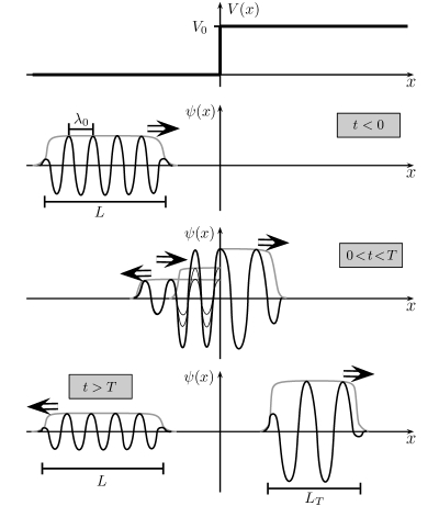
Figure 1: Visualization of a “plane-wave packet” interacting with the step potential shown in the top frame. The “$t<0$” frame shows a plane-wave packet of length $L$ and (central) wavelength $\lambda_{0}$ incident from the left. (Note that, strictly speaking, a plane-wave packet by definition has $L\gg\lambda_{0}$; the two length scales are inappropriately similar in the figure so that several other features will be more readily visible.) At $t=0$ the leading edge of the incident packet arrives at the origin and leading edges for the reflected and transmitted packets are produced. At $t=T$ the trailing edge of the incident packet arrives at the origin and trailing edges for the reflected and transmitted packets are produced. For $0<t<T$ the incident and reflected packets overlap in some (initially small, then bigger, then small again) region to the left of the origin. This is depicted in the “$0<t<T$” frame. Note that the amplitudes of the reflected and transmitted waves are determined by the usual boundary-matching conditions imposed at $x=0$. Finally, for $t>T$ the reflected and transmitted packets propagate away from the origin. Note that while the wavelength and packet length of the reflected wave matches those of the incident wave, the wavelength and packet length of the transmitted wave are respectively greater and smaller than those of the incident wave, owing to the different value of the potential energy to the right of the origin.

And the need to examine scattering in terms of (finite, normalizable) wave packets has long been recognized in the pilot-wave literature, which has included for example numerical studies of trajectories for Gaussian packets incident on various barriers. dh ; uu ; holland The use of Gaussian packets, however, tends to obscure the relationship to the standard textbook plane-wave calculation. There is no way to express the probabilities $P_{R}$ and $P_{T}$, for a narrow Gaussian packet, in anything like the simple form of Equations (13) and (14). And, in the pilot-wave picture, the complicated structure of the wave function during the scattering of the packet gives rise to equally complicated particle trajectories. So although one of course knows based on Equation (6) that the ensemble of possible particle trajectories will “follow” $\rho=|\psi|^{2}$, it is impossible to independently verify this without turning the problem over to a computer.

In the next section, we will develop a simple way to verify that, indeed, just the right fraction of the possible particle trajectories end up in the reflected and transmitted packets. To lay the ground for this, let us turn now to setting up a simple approach to reconciling the plane-wave and wave packet approaches. This should be of pedagogical interest even to those with no particular interest in the pilot-wave theory. To be clear, what follows is in no sense intended as a replacement for ordinary scattering theory. scattering The point is merely to show how, by considering incident packets with a particular special shape, the reflection and transmission probabilities can be read off in a trivial way from the packet amplitudes and widths.

Consider then an incident wave packet

$$\psi(x)=\phi(x)e^{ik_{0}x}$$ (15)

with a reasonably sharply-defined wave number $k_{0}$, but with a special, non-Gaussian, envelope profile $\phi(x)$. In particular, we imagine $\phi(x)$ to be nearly constant over a spatial region of length $L$, and zero outside this region. Then, as long as the (central) wavelength $\lambda_{0}=2\pi/k_{0}$ is very small compared to $L$ (actually, it should in addition be small compared to the length scale over which $\phi$ transitions to zero at the edges of the packet) the envelope function $\phi$ will maintain its shape and simply drift at the appropriate group velocity. Let us call this type of packet a “plane-wave packet”; its conceptual and analytical merit lies in the fact that, where it doesn’t vanish, it is well-approximated by a plane wave. planewave

In terms of such plane-wave packets, the scattering process can be understood as shown in Figure 1. Let us choose $t=0$ to be the time when the leading edge of the incident packet arrives at $x=0$. The incident packet has length $L$ and moves at the group velocity $v_{g}^{<}=\hbar k_{0}/m$. Thus, the packet’s trailing edge arrives at the origin at $t=T=L/v_{g}^{<}=Lm/\hbar k_{0}$. The whole scattering process then naturally breaks up into the following three time periods:

1. For $t<0$ the incident packet is propagating toward the barrier at $x=0$.

2. For $0<t<T$ the wave function in some (initially small, then bigger, then small again) region around $x=0$ is well-approximated by the plane-wave expressions of Equation (9).

3. For $t>T$ the incident packet has completely disappeared and there are reflected and transmitted packets propagating away from the barrier on either side.

It is now possible to understand the usual reflection and transmission probabilities in a remarkably simple way. To begin with, the incident packet should be properly normalized. Since it goes as $Ae^{ik_{0}x}$ over a region of length $L$, it is clear that

$$|A|=\frac{1}{\sqrt{L}}.$$ (16)

The total probability associated with the reflected packet can be found by multiplying its probability density $\rho_{R}=|B|^{2}$ by its length. Since the leading and trailing edges of the reflected packet are produced respectively when the leading and trailing edges of the incident packet arrive at the barrier – and since the reflected packet propagates in the same region as the incident packet so their group velocities are the same – the reflected packet has the same length, $L$, as the incident packet. Hence

$$P_{R}=|B|^{2}L=\frac{|B|^{2}}{|A|^{2}}=\frac{(k_{0}-\kappa_{0})^{2}}{(k_{0}+\kappa_{0})^{2}}$$ (17)

where in the last step we have used Equation (10) to relate the amplitude $B$ of the reflected packet to the amplitude $A$ of the incident one. The result here is of course in agreement with Equation (13).

The transmission probability can be calculated in a similar way. But here it is crucial to recognize that the group velocity for the $x>0$ region, $v_{g}^{>}=\hbar\kappa_{0}/m$, is smaller than the group velocity in the $x<0$ region. Thus, the position of the leading edge of the transmitted packet when the trailing edge is created at $x=0$, i.e., the length of the transmitted packet, is only

$$L_{T}=v_{g}^{>}\cdot T=v_{g}^{>}\cdot\frac{L}{v_{g}^{<}}=L\frac{\kappa_{0}}{k_{0}}.$$ (18)

That is, the transmitted packet is shorter, by a factor $\kappa_{0}/k_{0}$, than the incident and reflected packets. The total probability carried by the transmitted packet is then easily seen to be

$$P_{T}=L_{T}\,|C|^{2}=L|C|^{2}\frac{\kappa_{0}}{k_{0}}=\frac{\kappa_{0}}{k_{0}}\frac{|C|^{2}}{|A|^{2}}=\frac{4k_{0}\kappa_{0}}{(k_{0}+\kappa_{0})^{2}}$$ (19)

again in agreement with the earlier result. Note though, on this analysis, how the perhaps-puzzling factor of $\kappa_{0}/k_{0}$ in Equation (14) admits an intuitively clear origin in the relative lengths of the incident and transmitted packets.

Even in the context of conventional, textbook quantum theory, the “plane-wave packet” approach has several pedagogical merits. First, it allows the scattering process to be understood and visualized as a genuine, time-dependent process. Second, the reflection and transmission probabilities can be calculated without recourse to the somewhat cryptic and somewhat hand-waving device of taking ratios of certain hand-picked terms from the probability currents on each side. And finally, the explicit discussion of wave packets helps make clear that the results of the calculation – in particular the expressions for $P_{R}$ and $P_{T}$ – can be expected to be accurate only under the conditions (e.g., $L\gg\lambda_{0}$) assumed in the derivation. And of course the over-arching point is that all of this is accomplished while still using the mathematically simple plane-wave calculations: there is no particularly “messy business” and no need “to turn the problem over to a computer.”

In the following section, we will see the particular utility of the “plane-wave packet” approach in the context of the alternative pilot-wave picture.

III Particle Trajectories in the Pilot-Wave Theory

In the pilot-wave theory, the particle velocity is determined by the structure of the wave function in the vicinity of the particle, according to Equation (2). By considering a plane-wave packet as discussed in the previous section, we can see that there are several possible regions in which the particle may find itself. Let us consider these in turn.

To begin with, initially, the particle will be at some (random) location in the incident packet. Since, by assumption, the packet length $L$ is very large compared to the length scale associated with the packet’s leading and trailing edges, the particle is overwhelmingly likely to be at a location where the wave function in its immediate vicinity is given by

$$\psi_{I}(x)=Ae^{ik_{0}x}.$$ (20)

(Here and subsequently we omit for simplicity the time-dependent phase of the wave function, which plays no role.) It follows immediately that the particle’s velocity is

$$v_{I}=\frac{j_{I}}{\rho_{I}}=\frac{\frac{\hbar k_{0}}{m}|A|^{2}}{|A|^{2}}=\frac{\hbar k_{0}}{m}.$$ (21)

Note that this is the same as the group velocity of the incident packet. Thus, the particle will approach the barrier with the incident packet, indeed keeping its same position relative to the front and rear of the packet as both things (the wave and the particle) move.

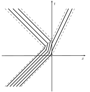
Figure 2: Space-time diagram showing a representative sample of possible particle trajectories for the case of a plane-wave packet incident from the left on a step potential. The leading and trailing edges of the various packets are indicated by the dashed grey lines. Particle trajectories are shown in black. In general, the particle simply moves at the group velocity along with the packet that is guiding it. In the (here, triangular) overlap region, however, the particle moves more slowly. This gives rise to a bifurcation of the possible trajectories, between those which arrive at the origin before being caught by the incident packet’s trailing edge (and thus end up moving away with the transmitted packet), and those which are caught by the incident packet’s trailing edge (and thus end up moving away with the reflected packet).

At some point – the exact time and place depending on its random initial position within the incident packet – the particle will encounter the leading edge of the reflected packet. It will then begin to move through the “overlap region” where both the incident and reflected waves are present:

$$\psi_{O}(x)=Ae^{ik_{0}x}+Be^{-ik_{0}x}.$$ (22)

Its velocity in this overlap region will be given by

$$v_{O}=\frac{j_{O}}{\rho_{O}}=\frac{\frac{\hbar k_{0}}{m}\left(|A|^{2}-|B|^{2}\right)}{|A|^{2}+|B|^{2}+2|A||B|\cos(2k_{0}x-\phi)}$$ (23)

where $\phi$ is the complex phase of $B$ relative to $A$ – zero in the case at hand. Here the right hand side is to be evaluated at each moment at the instantaneous location of the particle. This first-order differential equation for $X(t)$ is easily solved – more precisely, it is trivial to write an exact expression for $t(X)$ – but it is already clear from the above expression that the particle’s velocity will oscillate around an average “drift” value given by

$$\bar{v}_{O}=\frac{\hbar k_{0}}{m}\frac{|A|^{2}-|B|^{2}}{|A|^{2}+|B|^{2}}.$$ (24)

Since we are assuming that the packet length $L\gg\lambda_{0}=2\pi/k_{0}$, the particle’s velocity will (with overwhelming probability) oscillate above and below this average value many many times while it moves through the overlap region. It is thus an excellent approximation to simply ignore the oscillations and treat the particle as moving through the overlap region with a constant velocity $\bar{v}_{O}$.

There are two possible ways for the particle to escape from the overlap region. If it arrives at the origin, it will cross over into the region where only the transmitted wave

$$\psi_{T}(x)=Ce^{i\kappa_{0}x}$$ (25)

is present. It will then continue to move to the right with a velocity

$$v_{T}=\frac{j_{T}}{\rho_{T}}=\frac{\hbar\kappa_{0}}{m}$$ (26)

matching the group velocity of the transmitted packet.

The other possibility is that, while still in the overlap region, the trailing edge of the incident packet catches and surpasses the particle. It will then subsequently be guided exclusively by the reflected wave

$$\psi_{R}(x)=Be^{-ik_{0}x}.$$ (27)

Its velocity

$$v_{R}=\frac{j_{R}}{\rho_{R}}=-\frac{\hbar k_{0}}{m}$$ (28)

will match that of the reflected wave packet, with which it will propagate back out to the left.

It is helpful to visualize the family of possible particle trajectories on a space-time diagram; see Figure 2. Notice that a particle which happens to begin near the leading edge of the incident packet will definitely transmit, while particles beginning nearer the trailing edge of the incident packet will definitely reflect.

Although the dynamics here is completely deterministic, the theory makes statistical predictions because the initial position of a particular particle within its guiding wave is uncontrollable and unpredictable. Recall the “quantum equilibrium hypothesis” (QEH) according to which, for an ensemble of identically-prepared systems with initial wave function $\Psi(x,0)$, the initial particle positions will be random, with distribution given by Equation (5). It then follows, from the “equivariance” property described in the introduction, that $\rho=|\psi|^{2}$ will continue to describe the particles’ probability distribution for all $t$. The pilot-wave theory thus reproduces the exact statistical predictions of ordinary QM, but without any further axioms about measurement: whereas in ordinary QM, for example, the transmission probability $P_{T}$ (equal to the integral of $\rho$ across the transmitted packet) represents only the probability that the particle will appear there if a measurement is made, in the pilot-wave theory $P_{T}$ instead represents the probability that the particle really is there in the transmitted packet, ready to trigger a “click” in a detector should such a device happen to be present.

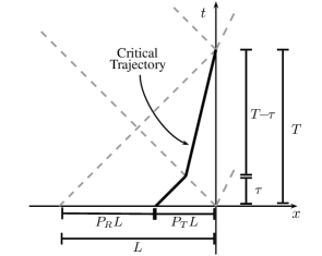
Figure 3: The critical trajectory, which arrives at the apex of the triangular overlap region on this space-time diagram, divides trajectories that transmit from those that reflect. The possible trajectories are distributed with uniform probability density throughout the incident packet, so the fraction of the total length $L$ of the packet that is in front of the critical trajectory represents the transmission probability, $P_{T}$. Equivalently, the critical trajectory is a distance $P_{T}\cdot L$ behind the incident packet’s leading edge. From $t=0$, it covers exactly half this distance before encountering the leading edge of the reflected packet. This occurs after a time $\tau=(P_{T}\cdot L/2)/(\hbar k_{0}/m)$. In traversing the overlap region, the critical trajectory then moves through the remaining distance $P_{T}\cdot L/2$. The time it takes is $T-\tau$, where $T=L/(\hbar k/m)$ is the time needed for the trailing edge of the incident packet to arrive at the origin. Equation (29) in the main text follows immediately by dividing this distance by this time.

As a concrete illustration of the equivariance property that guarantees the equivalence between the pilot-wave theory’s statistical predictions and those of ordinary quantum theory, let us derive the reflection and transmission probabilities directly from the particle trajectories and show that we indeed arrive again at the same expressions we found before by considering only the quantum wave. The key here is to examine in particular the “critical trajectory” which divides those trajectories which result in transmission, from those which result in reflection. This critical trajectory, by definition, arrives just at the apex of the triangular overlap region of Figure 2: particles on the leading-edge side of the critical trajectory will necessarily transmit, while particles on the trailing-edge side of the critical trajectory will necessarily reflect.

A zoomed-in image of the overlap region from Figure 2 is shown in Figure 3. As explained in the caption, the critical trajectory moves through the overlap region across a distance $P_{T}\cdot L/2$ where $P_{T}$ is the transmission probability. It does this in a time $T-\tau$ where $T=Lm/\hbar k_{0}$ and $\tau=(P_{T}\cdot L/2)/(\hbar k_{0}/m)$. It follows that the (average) velocity through the overlap region is

$$\bar{v}_{O}=\frac{P_{T}L/2}{\frac{Lm}{\hbar k_{0}}-\frac{P_{T}Lm}{2\hbar k_{0}}}=\frac{\hbar k_{0}}{m}\frac{P_{T}}{2-P_{T}}.$$ (29)

Equating this with the expression for the velocity in the overlap region worked out in Equation (24) gives

$$\frac{\hbar k_{0}}{m}\frac{P_{T}}{2-P_{T}}=\frac{\hbar k_{0}}{m}\frac{|A|^{2}-|B|^{2}}{|A|^{2}+|B|^{2}}$$ (30)

which can be solved for $P_{T}$ to give

$$P_{T}=\frac{|A|^{2}-|B|^{2}}{|A|^{2}}.$$ (31)

Using Equation (10) to put this in terms of the wave numbers $k_{0}$ and $\kappa_{0}$ of course gives back precisely Equation (14) for the transmission probability. And since $P_{R}=1-P_{T}$, Equation (13) is also implied again by the properties of the critical trajectory.

It is of course no surprise that we arrive at the same expressions for the transmission and reflection probabilities by considering the pilot-wave expression for the particle velocity in, especially, the crucial overlap region. But it is a clarifying confirmation of the sense in which the wave and particle evolutions are consistent as expressed in the equivariance property.

IV Tunneling through a rectangular barrier

To illustrate the more general applicability of the methods developed in the previous sections, let us analyze another standard textbook example – the tunneling of a particle through a classically forbidden region – from the pilot-wave perspective. Let the potential be given by

$$V(x)=\left\{\begin{array}[]{lc}V_{0}&\text{if }0<x<a\\ 0&\text{otherwise}\end{array}\right.$$ (32)

and let the particle, with a reasonably sharply defined energy $E<V_{0}$, be incident from the left. As before, we take the initial wave function $\Psi(x,0)$ to be a plane-wave packet with (central) wavelength $\lambda_{0}=2\pi/k_{0}$ (with $k_{0}=\sqrt{2mE/\hbar^{2}}$) and length $L\gg\lambda_{0}$. In addition, we assume here that the packet length $L$ is much greater than the width $a$ of the potential energy barrier. Then – letting now $\kappa_{0}=\sqrt{2m(V_{0}-E)/\hbar^{2}}$ – the wave function in the vicinity of the barrier will be given by

$$\psi(x)=\left\{\begin{array}[]{lcc}Ae^{ik_{0}x}+Be^{-ik_{0}x}&\text{if}&x<0\\ Ce^{-\kappa_{o}x}+De^{\kappa_{0}x}&\text{if}&0<x<a\\ Fe^{ik_{0}x}&\text{if}&x>a\end{array}\right.$$ (33)

for the overwhelming majority of the time when $\psi(x)$ near the barrier is nonzero. (In particular, $\psi(x)$ will differ substantially from the above expressions just when the leading edge of the incident packet first arrives at the barrier, and again when the trailing edge arrives there. But this will have negligible effect on our analysis since the probability for the particle to be too near the leading or trailing edges will be, for very large $L$, very small.)

Imposing the usual continuity conditions on $\psi(x)$ and its first derivative at $x=0$ and $x=a$ gives a set of four algebraic conditions on the amplitudes $A$, $B$, $C$, $D$, and $F$. Eliminating $C$ and $D$ allows the amplitudes of the reflected ($B$) and transmitted ($F$) packets to be written in terms of the amplitude $A$ of the incident packet:

$$\frac{B}{A}=\frac{-(\kappa_{0}^{2}+k_{0}^{2})\sinh(\kappa_{0}a)}{(\kappa_{0}^{2}-k_{0}^{2})\sinh(\kappa_{0}a)-2ik_{0}\kappa_{0}\cosh(\kappa_{0}a)}$$ (34)

and

$$\frac{F}{A}=\frac{-2ik_{0}\kappa_{0}}{(\kappa_{0}^{2}-k_{0}^{2})\sinh(\kappa_{0}a)-2ik_{0}\kappa_{0}\cosh(\kappa_{0}a)}e^{-ik_{0}a}.$$ (35)

Since the packet that develops on the downstream side of the barrier moves with the same group velocity as the incident packet, the transmitted packet length matches the incident packet length. The total probability associated with the transmitted packet – the “tunneling probability” – is thus

$$P_{T}=\frac{|F|^{2}}{|A|^{2}}=\frac{4k_{0}^{2}\kappa_{0}^{2}}{(\kappa_{0}^{2}+k_{0}^{2})^{2}\sinh^{2}(\kappa_{0}a)+4k_{0}^{2}\kappa_{0}^{2}}$$ (36)

with the corresponding reflection probability being

$$P_{R}=\frac{|B|^{2}}{|A|^{2}}=\frac{(\kappa_{0}^{2}+k_{0}^{2})^{2}\sinh^{2}(\kappa_{0}a)}{(\kappa_{0}^{2}+k_{0}^{2})^{2}\sinh^{2}(\kappa_{0}a)+4k_{0}^{2}\kappa_{0}^{2}}.$$ (37)

As before, these results can be understood in terms of the particle trajectories as well. In general the trajectories are very similar to those from the earlier example. While the incident and reflected packets are both present to the left of the barrier, an overlap region is set up in which the motion of the incoming particle is slowed. The particle velocity in this region is again described by Equation (23), although now there is a nontrivial complex phase between the amplitudes $B$ and $A$:

$$\phi=\tan^{-1}\left(\frac{2k_{0}\kappa_{0}\cosh(\kappa_{0}a)}{(\kappa_{0}^{2}-k_{0}^{2})\sinh(\kappa_{0}a)}\right).$$ (38)

The average drift velocity through the overlap region, however, remains as in Equation (24), so the analysis surrounding Figure 3 still applies and we have again that the transmission (or here, tunneling) probability as determined by the critical trajectory is

$$P_{T}=\frac{|A|^{2}-|B|^{2}}{|A|^{2}}$$ (39)

in agreement with the result arrived at by considering just the waves. This again confirms that the distribution of possible particle trajectories evolves in concert with the wave intensity $\rho$ such that Equation (6) remains true at all times.

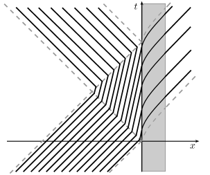
Figure 4: Space-time diagram showing a representative sample of possible particle trajectories for the case of a plane-wave packet incident from the left on a rectangular potential barrier. Particles beginning near the leading edge of the incident packet will tunnel through the barrier and emerge on the far side. The unusual accelerating character of the trajectories in the (here, grey shaded) classically-forbidden region – indeed the mere presence of trajectories here – reflects the highly non-classical nature of the law of motion for the particle. (Note that the analysis in the main text assumes that the incident packet length $L$ is very large compared to the barrier width $a$. This separation of length scales is not accurately depicted in the Figure, in order that the qualitative nature of the trajectories in all relevant regions can be visualized simultaneously.)

The nature of the pilot-wave theory particle trajectories in the classically-forbidden region (CFR) is of some interest. The wave function in the CFR goes as

$$\psi_{\text{CFR}}(x)=Ce^{-\kappa_{0}x}+De^{\kappa_{0}x}$$ (40)

where the four algebraic conditions mentioned just prior to Equation (34) imply that

$$\frac{D}{C}=\frac{(\kappa_{0}+ik_{0})^{2}}{\kappa_{0}^{2}+k_{0}^{2}}e^{-2\kappa_{0}a}=e^{i\theta}e^{-2\kappa_{0}a}$$ (41)

where the relative phase $\theta$ is given by

$$\theta=2\tan^{-1}(k_{0}/\kappa_{0}).$$ (42)

The fact that the relative complex phase of $D$ and $C$ is not zero is crucial: if this were zero, the probability current $j$ and hence the particle velocity would vanish, and it would be impossible for the particles to tunnel across the barrier. Instead, though, we have that

$$j_{\text{CFR}}(x)=\frac{2\hbar\kappa_{0}}{m}|C|^{2}\sin(\theta)e^{-2\kappa_{0}a}$$ (43)

and

$$\frac{\rho_{\text{CFR}}(x)}{|C|^{2}}=e^{-2\kappa_{0}x}+e^{-4\kappa_{0}a}e^{2\kappa_{0}x}+2e^{-2\kappa_{0}a}\cos(\theta)$$ (44)

so that the particle velocity is given by

$$v_{\text{CFR}}(x)=\frac{\hbar\kappa_{0}}{m}\frac{\sin(\theta)}{\cos(\theta)+\cosh\left[2\kappa_{0}(a-x)\right]}.$$ (45)

Thus, particles speed up as they cross (from $x=0$ to $x=a$) over the CFR.

Figure 4 displays the behavior of a representative sample of particle trajectories. The overall pattern is similar to the case of scattering from the step potential: particles that begin near the trailing edge of the incident packet will be swept up by the reflected packet before reaching $x=0$, while those which begin nearer the leading edge of the incident packet will reach the barrier, tunnel across it, and emerge with the transmitted packet.

V Discussion

We have analyzed two standard textbook cases of one-dimensional quantum mechanical scattering and tunneling from the point of view of the de Broglie - Bohm pilot-wave theory. In particular, we have shown how the standard textbook expressions for the reflection and transmission/tunneling probabilities – calculated using infinitely-extended plane-wave states – can instead be understood as arising from a certain type of idealized, non-Gaussian incident wave packet. We then took advantage of this “plane-wave packet” approach to generate a tractable, indeed quite simple, picture of how the particle trajectories in the pilot-wave theory develop.

It is hoped that the plane-wave packet approach might prove clarifying for students learning standard textbook quantum mechanics. It is also hoped that introducing the pilot-wave theory through standard textbook examples will make it easier for teachers to present the range of available interpretive options clearly and effectively to students. Recent work has shown that modern physics students have particular difficulty with conceptual questions involving issues of interpretation wuttiprom – a finding that is hardly surprising given that physics teachers themselves have divergent views on interpretive questions and their place in the curriculum. baily These questions deserve to be discussed more explicitly and more carefully, and it seems natural to do so in the context of the kinds of example problems that students encounter in such courses anyway.

Despite its not being suggested as an option in the textbook or lectures, several of the students interviewed in Ref. baily, seem to have independently developed a pilot-wave type understanding of single-particle interference phenomena. Many eminent physicists have also found a pilot-wave ontology to be the natural way to account for puzzling quantum effects. Here, for example, is J.S. Bell on single-particle interference experiments:

“While the founding fathers agonized over the question

‘particle’ or ‘wave’

de Broglie in 1925 proposed the obvious answer

‘particle’ and ‘wave’.

Is it not clear from the smallness of the scintillation on the screen that we have to do with a particle? And is it not clear, from the diffraction and interference patterns, that the motion of the particle is directed by a wave? De Broglie showed in detail how the motion of a particle, passing through just one of two holes in [the] screen, could be influenced by waves propagating through both holes. And so influenced that the particle does not go where the waves cancel out, but is attracted to where they cooperate. This idea seems to me so natural and simple, to resolve the wave-particle dilemma in such a clear and ordinary way, that it is a great mystery to me that it was so generally ignored.” bell6

In an earlier paper, Bell asked:

“Why is the pilot wave picture ignored in text books? Should it not be taught, not as the only way, but as an antidote to the prevailing complacency? To show that vagueness, subjectivity, and indeterminism are not forced on us by experimental facts, but by deliberate theoretical choice?” bellwhy

If current physicists answered these questions, the majority would probably cite two factors, both of which involve some confusion and mis-information. First, there is the oft-repeated charge that the pilot-wave theory involves an ad hoc and cumbersome additional field – the so-called “quantum potential” – to guide the particle. The theory has indeed been presented in such a form by Bohm and others. uu ; holland But as the examples in the body of the present work should help make clear, this is an entirely unnecessary addition to the “minimalist” pilot-wave theory, in which the field guiding the particle is none other than the usual quantum mechanical wave function obeying the usual Schrödinger equation.

The second factor typically cited by critics of the pilot-wave theory is its non-local character and the associated alleged incompatibility with relativity. It is true, as discussed just after Equation (4) above, that the pilot-wave theory is explicitly non-local. What the critics forget, however, is that ordinary quantum mechanics is also a non-local theory: already in its account of the simple one-particle scattering phenomena discussed here, orthodox quantum theory needs additional postulates – in particular the infamous and manifestly non-local collapse postulate – to explain what is empirically observed. The truth is that, as we know from Bell, no local theory can be empirically adequate. belltheorem So rejecting candidate interpretations on the basis of their non-local character is hardly appropriate. Nevertheless, it is interesting that the conventional wisdom on this point is completely backwards: the pilot-wave theory is actually less non-local than ordinary quantum theory in the sense that it (unlike the orthodox theory) can at least account for the results of one-particle scattering/tunneling/interference experiments in a completely local way.

It is thus hoped not only that the examples presented here will provide a simple concrete way for the alternative pilot-wave picture to be introduced to students, but also that the examples will help overturn some unfortunate and widely-held misconceptions about the theory. And of course it should be noted that the pilot-wave theory is just one of several alternatives to the usual Copenhagen-inspired theory that appears in most textbooks. There is, for example, also the many-worlds (“Everettian”) theory, the spontaneous collapse (“GRW”) theory, the consistent (or decoherent) histories approach, and many others. As someone who thinks that these questions – about the physics behind the quantum formalism – are meaningful, important, fascinating, controversial, and too-often hidden under a shroud of unspeakability, I would like to see all of these interpretations more widely understood and discussed by physicists, both in and out of the classroom. (Some suggestions for introducing the issues and options to students can be found in Ref. suggestions, .) At the end of the day, though, I cannot help but agree with Bell, who, after reviewing “Six possible worlds [i.e., interpretations] of quantum mechanics”, concluded that “the pilot wave picture undoubtedly shows the best craftsmanship.” bell6 Hopefully the examples discussed above will help others appreciate why.

- (1) An English translation of Louis de Broglie’s 1927 pilot-wave theory can be found in G. Bacciagalluppi and A. Valentini, Quantum Theory at the Crossroads, Cambridge, 2009. David Bohm’s 1952 re-discovery of the theory is presented in “A Suggested Interpretation of the Quantum Theory in terms of Hidden Variables, I and II”, Physical Review, 85 (1952), pp. 166-193. A more contemporary overview, with further references, can be found at plato.stanford.edu/entries/qm-bohm.
- (2) J.S. Bell, “Beables for Quantum Field Theory” (1984) in Speakable and Unspeakable in Quantum Mechanics, 2nd ed., Cambridge, 2004.
- (3) See for example R.G. Newton, Scattering Theory of Waves and Particles, 2nd Ed., Springer, Berlin / Heidelberg / New York, 1982; M. Reed and B. Simon, Methods of Modern Mathematical Physics III: Scattering Theory, San Diego, Academic Press, 1979.
- (4) J.S. Bell, “On the Einstein-Podolsky-Rosen Paradox”, Physics 1 (1964) 195-200. Reprinted in Bell, 2004, op cit. For a contemporary systematic review of Bell’s Theorem, see S. Goldstein, T. Norsen, D. Tausk, and N. Zanghi, “Bell’s Theorem” at scholarpedia.org/article/Bell%27s_theorem
- (5) D. Dürr, S. Goldstein, and N. Zanghi, “Quantum Equilibrium and the Origin of Absolute Uncertainty”, Journal of Statistical Physics 67, pp. 843-907.
- (6) Ibid. See also M.D. Towler, N.J. Russell, and A. Valentini, “Time scales for dynamical relaxation to the Born rule”, Proceedings of the Royal Society A, 468 (2012), pp. 990-1013.
- (7) J.S. Townsend, Quantum Physics: A Fundamental Approach to Modern Physics, University Science Books, Sausalito, California, 2010.
- (8) D.J. Griffiths, Introduction to Quantum Mechanics, Prentice Hall, New Jersey, 1995, p. 58 .
- (9) R. Shankar, Principles of Quantum Mechanics, Second Edition, Springer, 1994.
- (10) C. Dewdney and B.J. Hiley, “A Quantum Potential Description of One-Dimensional Time-Dependent Scattering From Square Barriers and Square Wells” Foundations of Physics, Vol. 12, 1982, pp. 27-48.
- (11) D. Bohm and B.J. Hiley, The Undivided Universe, Routledge, London and New York, 1993, pp. 73-8.
- (12) P. Holland, The Quantum Theory of Motion, Cambridge University Press, 1993, pp. 198-203 (and references therein).
- (13) For a rather different (alternative) approach to scattering that also uses the terminology “plane-wave packet” see Stuart C. Althorpe, “General time-dependent formulation of quantum scattering theory”, Physical Review A, 69, 042702 (2004).
- (14) S. Wuttiprom, M. D. Sharma, I. D. Johnston, R. Chitaree, and C. Soankwan, “Development and Use of a Conceptual Survey in Introductory Quantum Physics”, Int. J. Sci. Educ. 31, 631-654 (2009).
- (15) C. Baily and N. Finkelstein, “Refined characterization of student perspectives on quantum physics”, Phys. Rev. ST Physics Ed. Research 6, 020113, pp. 1-11 (2010)
- (16) J.S. Bell, “Six Possible Worlds of Quantum Mechanics,” 1986, reprinted in Bell, 2004, op cit. (Note: ellipsis in original.)
- (17) J.S. Bell, “On the impossible pilot wave,” 1982, reprinted in Bell, 2004, op cit.
- (18) Bell’s paper, “Six Possible Worlds of Quantum Mechanics”, op. cit., reviews the relevant phenomena of single-particle interference and then surveys six different extant interpretations. It is an extremely accessible introduction to the nature (and existence) of the controversies, and I have often used it as the basis for a one-class-period discussion in a sophomore-level modern physics course. At a slightly more technical level, Sheldon Goldstein’s two-part Physics Today article [March, 1998, pp. 42-46 and April, 1998, pp. 38-42] gives an extremely clear presentation of three attempts to formulate a “Quantum Theory Without Observers” and an illuminating explanation for why such a thing should be desirable in the first place. For students who want to explore foundational issues (EPR, Bell, etc.) and their emerging applications (quantum cryptography, computation, etc.) in more depth, I would recommend GianCarlo Ghirardi’s lucid book, Sneaking a Look at God’s Cards, Revised Edition, Gerald Malsbary, trans., Princeton University Press, 2005.