A Relative Entropy Rate Method for Path Space Sensitivity Analysis of Stationary Complex Stochastic Dynamics

Abstract

We propose a new sensitivity analysis methodology for complex stochastic dynamics based on the Relative Entropy Rate. The method becomes computationally feasible at the stationary regime of the process and involves the calculation of suitable observables in path space for the Relative Entropy Rate and the corresponding Fisher Information Matrix. The stationary regime is crucial for stochastic dynamics and here allows us to address the sensitivity analysis of complex systems, including examples of processes with complex landscapes that exhibit metastability, non-reversible systems from a statistical mechanics perspective, and high-dimensional, spatially distributed models. All these systems exhibit, typically non-gaussian stationary probability distributions, while in the case of high-dimensionality, histograms are impossible to construct directly. Our proposed methods bypass these challenges relying on the direct Monte Carlo simulation of rigorously derived observables for the Relative Entropy Rate and Fisher Information in path space rather than on the stationary probability distribution itself. We demonstrate the capabilities of the proposed methodology by focusing here on two classes of problems: (a) Langevin particle systems with either reversible (gradient) or non-reversible (non-gradient) forcing, highlighting the ability of the method to carry out sensitivity analysis in non-equilibrium systems; and, (b) spatially extended Kinetic Monte Carlo models, showing that the method can handle high-dimensional problems.

I Introduction

In this paper we propose the Relative Entropy Rate as a sensitivity analysis tool for complex stochastic dynamics, based on information theory and non-equilibrium statistical mechanics methods. These calculations become computationally feasible at the stationary process regime and involve the calculation of suitable observables in path space for the Relative Entropy Rate and the corresponding Fisher Information Matrix. The stationary regime, i.e. stochastic dynamics where the initial probability distribution is the stationary distribution reached after long-time integration, is especially crucial for complex systems: it includes dynamic transitions between metastable states in complex, high-dimensional energy landscapes, intermittency, as well as Non Equilibrium Steady States (NESS) for non-reversible systems, while at this regime we also construct phase diagrams for complex systems. Hence their sensitivity analysis is a crucial question in determining which parameter directions are the most/least sensitive to perturbations, uncertainty or errors resulting from parameter estimation. Recently there has been significant progress in developing sensitivity analysis tools for low-dimensional stochastic processes at the transient regime, such as well-mixed chemical reactions. Some of the mathematical tools included discrete derivatives Gunawan et al. (2005), Girsanov transformations Nakayama et al. (1994); Plyasunov and Arkin (2007), polynomial chaos Kim et al. (2007), and coupling of stochastic processes Rathinam et al. (2010).

On the other hand, it is often the case that we are interested in the entire probability density function (PDF), which in nonlinear and/or discrete systems is typically non-Gaussian, and not only in a few moments, due to the significance of rare/tail events. For example, it was recently shown that in catalytic reactions the most kinetically relevant configurations are occurring rarely, and correspond to overlapping tails of (non-Gaussian) PDFs Wu et al. (2012). In that latter direction, there is a broad recent literature relying on information theory tools, where sensitivity is estimated by using the Relative Entropy and the Fisher Information between PDFs, see for instance Liu et al. (2006); N. Lüdtke and S. Panzeri and M. Brown and D. S. Broomhead and J. Knowles and M. A. Montemurro and D. B. Kell (2008); Majda and Gershgorin (2010, 2011); Komorowski et al. (2011). In particular, such methods were introduced for the study of the sensitivity of PDFs to parameters in climate models Majda and Gershgorin (2010); there the PDFs structure is known as it is obtained through an entropy maximization subject to constraints. Knowing the form of the PDF allows to carry out calculations such as obtaining a Fisher Information Matrix (FIM), which in turn identifies the most sensitive parameter directions. On the other hand, the sensitivity of stochastic dynamics can be studied by using the FIM Komorowski et al. (2011). There the authors are employing a linearization of the stochastic evolution around the nonlinear mean field equation and as a result the form of the PDF is again known, and more precisely it is Gaussian hence the FIM can be directly computed. Although there are regimes where this approximation is applicable (short times, systems with a single steady state, etc.), for systems with nontrivial long-time dynamics, e.g. metastable, it is not correct as large deviation arguments Doering et al. (2007) show, or even explicitly available formulas for escape times Hanggi et al. (1984). Similar issues with non-gaussianity in the long time dynamics arise in stochastic systems with strongly intermittent behavior Katsoulakis et al. (2006).

Some of these challenges will be addressed through the proposed methods which we present next in the context of kinetic Monte Carlo models although similar challenges and ideas are relevant to all other stochastic molecular simulation methods. For example, we discuss in Section V.C the sensitivity of algorithms for the numerical integration of Langevin dynamics. Moreover, kinetic Monte Carlo methods involving surface chemistry are formulated in terms of continuous time Markov chains (jump processes) on a spatial lattice domain ${\Lambda}_{N}$: at each lattice site $x\in{\Lambda}_{N}$ there is a state space $\Sigma=\{0,1,\dots,{K}\}$ describing different chemical species (interacting particles), where the simplest case $K=1$ represents the well-known lattice-gas model Liggett (1985). The process $\sigma_{t}$ is defined as a continuous time Markov Chain (CTMC) on the (high-dimensional) state space ${\mathcal{S}_{N}}=\Sigma^{{\Lambda}_{N}}$ and mathematically it is defined completely by specifying the local transition rates $c^{\theta}(\sigma,\sigma^{\prime})$ where $\theta\in\mathbb{R}^{k}$ is a vector of the model parameters. The transition rates determine the updates (jumps) from any current state $\sigma_{t}=\sigma$ to a (random) new state $\sigma^{\prime}$ and concrete examples of spatial physicochemical models are considered in Section V.D. From the local transition rates one defines the total rate $\lambda^{\theta}(\sigma)=\sum_{\sigma^{\prime}}c^{\theta}(\sigma,\sigma^{\prime})$, which is the intensity of the exponential waiting time for a jump from the state $\sigma$. The transition probabilities are $p^{\theta}(\sigma,\sigma^{\prime})=\frac{c^{\theta}(\sigma,\sigma^{\prime})}{\lambda^{\theta}(\sigma)}$. The basic simulation tool for these lattice jump processes is kinetic Monte Carlo (KMC) with a wide range of applications from crystal growth, to catalysis, to biology, see for instance Chatterjee and Vlachos (2007).

Relative Entropy Rate : In simulations of dynamic transitions between metastable states on high-dimensional energy landscapes or of NESS we are interested in the sensitivity of stationary processes, i.e., processes for which the initial probability distribution is the stationary one (reached after long-time integration). Mathematically, we want to assess the sensitivity of the CTMC $\{\sigma_{t}\}_{t\geq 0}$ with local transition rates $c^{\theta}(\sigma,\sigma^{\prime})$ to a perturbation $\epsilon\in\mathbb{R}^{k}$ in the parameter vector $\theta$ giving rise to a process $\{\widetilde{\sigma}_{t}\}_{t\geq 0}$ with local transition rates $c^{\theta+\epsilon}(\sigma,\sigma^{\prime})$, when the initial data are sampled from the respective stationary probability distribution. The error analysis in the context of the long-time behavior is developed in terms of the relative entropy,

$$\mathcal{R}\left({{Q_{[0,T]}^{\theta}}}{\,|\,}{{Q_{[0,T]}^{\theta+\epsilon}}}\right)=\int\log\left(\frac{d{Q_{[0,T]}^{\theta}}}{d{Q_{[0,T]}^{\theta+\epsilon}}}\right)\,dQ_{[0,T]}^{\theta}\,,$$ (1)

where $Q_{[0,T]}^{\theta}$ (resp. $Q_{[0,T]}^{\theta+\epsilon}$) is the path space probability measures of $\{\sigma_{t}\}_{t\geq 0}$ (resp. $\{\widetilde{\sigma}_{t}\}_{t\geq 0}$) in the time interval $[0,T]$. In the case these probability measures have corresponding probability densities $q^{\theta}$ and $q^{\theta+\epsilon}$, (1) becomes $\mathcal{R}\left({{Q_{[0,T]}^{\theta}}}{\,|\,}{{Q_{[0,T]}^{\theta+\epsilon}}}\right)=\int q^{\theta}\log\left(\frac{q^{\theta}}{q^{\theta+\epsilon}}\right)$. A key property of the relative entropy $\mathcal{R}\left({P}{\,|\,}{Q}\right)$ is that $\mathcal{R}\left({P}{\,|\,}{Q}\right)\geq 0$ with equality if and only if $P=Q$, which allows us to view relative entropy as a “distance” (more precisely a semi-metric) between two probability measures $P$ and $Q$. Moreover, from an information theory perspective Cover and Thomas (1991), the relative entropy measures loss/change of information, e.g. in our context for the process $\{\sigma_{t}\}_{t\geq 0}$ associated with the parameter vector $\theta$, with respect to the process $\{\widetilde{\sigma}_{t}\}_{t\geq 0}$ associated with the parameter vector $\theta+\epsilon$. Relative entropy for high-dimensional systems was used as measure of loss of information in coarse-grainingKatsoulakis and Trashorras (2006); Katsoulakis et al. (2007); Arnst and Ghanem (2008), and sensitivity analysis for climate modeling problems Majda and Gershgorin (2010).

Starting from (1), by Girsanov’s formula we obtain an explicit expression for the corresponding Radon-Nikodym derivative

$$\frac{dQ_{[0,T]}^{\theta}}{dQ_{[0,T]}^{\theta+\epsilon}}(\{\sigma_{t}\}) =\exp\Big{\{}\sum_{s\leq T}\log\frac{\lambda^{\theta}(\sigma_{s-})p^{\theta}(\sigma_{s-},\sigma_{s})}{\lambda^{\theta+\epsilon}(\sigma_{s-})p^{\theta+\epsilon}(\sigma_{s-},\sigma_{s})}$$ (2)

$$-\int_{0}^{T}[\lambda^{\theta}(\sigma_{s})-\lambda^{\theta+\epsilon}(\sigma_{s})]\,ds\Big{\}}\,,$$

on any path of the process $\{\sigma_{t}\}_{t\in[0,T]}$ in terms of the jump rates and transition probabilities of both process, under suitable non-degeneracy conditions Kipnis and Landim (1999). Notice that $\sigma_{s-}$ denotes the left-hand limit of $\sigma_{s}$ at a jump instance $s$. Following calculations regarding the related quantity of entropy production in non-equilibrium statistical mechanics Maes et al. (2000), we can show that when the initial distribution $\sigma_{0}\sim\mu^{\theta}$ where $\mu^{\theta}$ (resp. $\mu^{\theta+\epsilon}$) is the stationary probability disturbution of $\{\sigma_{t}\}_{t\geq 0}$ (resp. $\{\widetilde{\sigma}_{t}\}_{t\geq 0}$), then the relative entropy formula simplifies dramatically in two parts, one pure equilibrium (scaling as $\mathcal{O}(1)$) and one capturing the stationary dynamics (scaling as $\mathcal{O}(T)$):

$$\mathcal{R}\left({{Q_{[0,T]}^{\theta}}}{\,|\,}{{Q_{[0,T]}^{\theta+\epsilon}}}\right)=T\mathcal{H}\left({{Q_{[0,T]}^{\theta}}}{\,|\,}{{Q_{[0,T]}^{\theta+\epsilon}}}\right)+\mathcal{R}\left({\mu^{\theta}}{\,|\,}{\mu^{\theta+\epsilon}}\right),$$ (3)

where $\mathcal{R}\left({\mu^{\theta}}{\,|\,}{\mu^{\theta+\epsilon}}\right)$ is the relative entropy between the stationary probabilities, while

$$\mathcal{H}\left({{Q_{[0,T]}^{\theta}}}{\,|\,}{{Q_{[0,T]}^{\theta+\epsilon}}}\right)=\mathbb{E}_{\mu^{\theta}}\Big{[}\sum_{\sigma^{\prime}}\lambda^{\theta}(\sigma)p^{\theta}(\sigma,\sigma^{\prime})$$ (4)

$$\times\log\frac{\lambda^{\theta}(\sigma)p^{\theta}(\sigma,\sigma^{\prime})}{\lambda^{\theta+\epsilon}(\sigma)p^{\theta+\epsilon}(\sigma,\sigma^{\prime})}-(\lambda^{\theta}(\sigma)-\lambda^{\theta+\epsilon}(\sigma))\Big{]}\,,$$

where $\mathbb{E}_{\mu^{\theta}}$ denotes the expected value with respect to the probability $\mu^{\theta}$. In (3), we immediately notice that a most relevant quantity to describe the change of information content upon perturbation of model parameters of a stochastic process is the $\mathcal{O}(T)$ term, which can be thought as a relative entropy per unit time while on the other hand, the term $\mathcal{R}\left({\mu^{\theta}}{\,|\,}{\mu^{\theta+\epsilon}}\right)$ becomes unimportant as $T$ grows.

We will refer from now on to the quantity (LABEL:relent2) as the Relative Entropy Rate (RER), which can be thought as the change in information per unit time. Notice that RER has the correct time scaling since it is actually independent of the interval $[0,T]$. Furthermore, (LABEL:relent2) provides a computable observable that can be sampled from the steady state $\mu^{\theta}$ in terms of conventional KMC, bypassing the need for a histogram or an explicit formula for the high-dimensional probabilities involved in (1). Finally, the fact that in stationary regimes, when $T\gg 1$ in (3), the term $\mathcal{R}\left({\mu^{\theta}}{\,|\,}{\mu^{\theta+\epsilon}}\right)$ becomes unimportant, is especially convenient: $\mu^{\theta}$ and $\mu^{\theta+\epsilon}$ are typically not known explicitly in non-reversible systems, for instance in spatially distributed reaction KMC or non-reversible Langevin dynamics considered here as examples.

Fisher Information Matrix on Path Space : An attractive approach to sensitivity analysis that is rigorously based on relative entropy calculations is the Fisher Information Matrix. Indeed, assuming smoothness in the parameter vector, it is straightforward to obtain the expansion of (1) Cover and Thomas (1991); Abramov et al. (2005),

$$\mathcal{R}\left({{Q_{[0,T]}^{\theta}}}{\,|\,}{{Q_{[0,T]}^{\theta+\epsilon}}}\right)=\frac{1}{2}\epsilon^{T}\mathbf{F}_{\mathcal{R}}(Q_{[0,T]}^{\theta})\epsilon+O(|\epsilon|^{3})\,,$$ (5)

where the Fisher Information Matrix (FIM) is defined as the Hessian of the relative entropy:

$$\mathbf{F}_{\mathcal{R}}(Q_{[0,T]}^{\theta})=\left.\nabla_{\epsilon}^{2}\mathcal{R}\left({{Q_{[0,T]}^{\theta}}}{\,|\,}{{Q_{[0,T]}^{\theta+\epsilon}}}\right)\right|_{\epsilon=0}\,.$$ (6)

As (5) readily suggests, relative entropy is locally a quadratic function of the parameter vector $\theta$. Thus spectral analysis of $\mathbf{F}_{\mathcal{R}}$–provided the matrix is available–would allow us to identify which parameter directions are the most/least sensitive to perturbations, uncertainty or errors resulting from parameter estimation. The source of such uncertainties could be related to the assimilation of experimental data Rao et al. (2009) or finer scale numerical simulation, e.g. Density Functional Theory computations in the case of molecular simulations Braatz et al. (2006). More specifically, the knowledge of the Fisher Information Matrix not only provides a gradient-free method for sensitivity analysis, but allows to address questions of parameter identifiability Rothenberg (1971); Komorowski et al. (2011) and optimal experiment design Emery and Nenarokomov (1998); Prasad et al. (2010). However, the FIM $\mathbf{F}_{\mathcal{R}}$ in (6) is not accessible computationally in general, nevertheless analytic calculations can be performed at equilibrium (e.g., in ergodic systems when $T\to\infty$) under the assumption or the explicit knowledge of the stationary distribution $\mu$. An example of such a calculation is under the assumption of a Gaussian distribution with the mean $m(\theta)$ and the covariance matrix $\Sigma(\theta)$ in which case the matrix $\mathbf{F}_{\mathcal{R}}$ is computed in terms of derivatives of the mean and covariance matrix Komorowski et al. (2011).

On the other hand (3) provides a different perspective to these issues, giving rise to a computable observable for the path space Fisher Information Matrix that includes transition rates rather than just the stationary PDFs. Indeed, by combining (3) and (5) we obtain the following expansion for the dominant, $O(T)$ term in (3):

$$\mathcal{H}\left({Q_{[0,T]}^{\theta}}{\,|\,}{Q_{[0,T]}^{\theta+\epsilon}}\right)=\frac{1}{2}\epsilon^{T}\mathbf{F_{\mathcal{H}}}(Q_{[0,T]}^{\theta})\epsilon+O(|\epsilon|^{3})\,,$$ (7)

where the Fisher Information Matrix per unit time, $\mathbf{F_{\mathcal{H}}}(Q_{[0,T]}^{\theta})$, has the explicit form

$$\mathbf{F_{\mathcal{H}}}(Q_{[0,T]}^{\theta}) =\mathbb{E}_{\mu^{\theta}}\Big{[}\sum_{\sigma^{\prime}}c^{\theta}(\sigma,\sigma^{\prime})$$ (8)

$$\times\nabla_{\theta}\log c^{\theta}(\sigma,\sigma^{\prime})\nabla_{\theta}\log c^{\theta}(\sigma,\sigma^{\prime})^{T}\Big{]}\,,$$

where $c^{\theta}(\sigma,\sigma^{\prime})=\lambda^{\theta}(\sigma)p^{\theta}(\sigma,\sigma^{\prime})$. Fisher Information Matrices given by (6) and (8) are straightforwardly related through $\lim_{T\rightarrow\infty}\frac{1}{T}\mathbf{F}_{\mathcal{R}}=\mathbf{F_{\mathcal{H}}}$. It is clear from (8) that the Fisher Information Matrix, just like the Relative Entropy Rate (LABEL:relent2), is merely an observable that can be sampled using KMC algorithms.

The previous discussion suggests that the proposed approach to sensitivity analysis is expected to have the following features:

1. It is rigorously valid for the sensitivity of long-time, stationary dynamics in path space, including for example metastable dynamics in a complex landscape.

2. It is a gradient-free sensitivity analysis method which does not require the knowledge of the equilibrium PDFs, as (6) is replaced with a computable observable (8), that contains explicitly information for local dynamics.

3. It is suitable for non-equilibrium systems from a statistical mechanics perspective; for example, non-reversible processes, such as spatially extended reaction-diffusion Kinetic Monte Carlo, where the structure of the equilibrium PDF is unknown and is typically non-Gaussian.

4. A key enabling tool for implementing the proposed methodology in high-dimensional stochastic systems is molecular simulation methods such as KMC or Langevin solvers which can sample the observables (LABEL:relent2) and (8), and in particular their accelerated or scalable versions Gillespie (2001); Chatterjee and Vlachos (2007); Plimpton et al. (2009); Plimpton and Thompson (2012); Arampatzis et al. (2012).

Indeed, we demonstrate these features by presenting three examples addressing different points: (a) the well-mixed bistable reaction system known as the Schlögl model which also serves as a benchmark; (b) a Langevin particle system with either reversible or non-reversible forcing, that demonstrates the ability of the proposed method to carry out sensitivity analysis in non-equilibrium systems; and, (c) a spatially extended KMC model for $CO$ oxidation known as the Ziff-Gulari-Barshad (ZGB) model. Such reaction-diffusion models are typically non-reversible, hence the sensitivity tools we propose here are highly suitable. Regarding this last class of problems, we note that in more accurate, state-of-the-art KMC models with a large number of parameters Hansen and Neurock (2000); Meskine et al. (2009); Stamatakis et al. (2011), kinetic parameters are estimated through density functional theory (DFT) calculations, hence sensitivity analysis is a crucial step in determining the parameters that need to be calculated with greater accuracy.

The paper is organized as follows: in Section II we present the derivation of the Relative Entropy Rate and its corresponding Fisher Information Matrix for discrete-time Markov chains while Section III the same observables for continuous-time Markov processes (i.e., (3), (LABEL:relent2) and (8)) are derived. Section IV generalizes the RER and the FIM to time-periodic, inhomogeneous Markov processes as well as to semi-Markov processes. Statistical estimators and numerical examples in Section V demonstrate the efficiency of the proposed sensitivity method, while Section VI concludes the paper.

II Discrete Time Markov Chains

Let $\{\sigma_{m}\}_{m\in\mathbb{Z}^{+}}$ be a discrete-time time-homogeneous Markov chain with separable state space $E$. The transition probability kernel of the Markov chain denoted by $P^{\theta}(\sigma,d\sigma^{\prime})$ depends on the parameter vector $\theta\in\mathbb{R}^{k}$. Assume that the transition kernel is absolute continuous with respect to (w.r.t.) the Lebesgue measureNote (1) and the transition probability density function $p^{\theta}(\sigma,\sigma^{\prime})$ is always positive for all $\sigma,\sigma^{\prime}\in E$ and for all $\theta\in\mathbb{R}^{k}$. We further assume that $\{\sigma_{m}\}_{m\in\mathbb{Z}^{+}}$ has a unique stationary probability distribution denoted by $\mu^{\theta}(\sigma)$. Exploiting the Markov property, the path probability distribution $Q_{0,M}^{\theta}$ for the path $\{\sigma_{m}\}_{m=0}^{M}$ at the time horizon $0,...,M$ starting from the stationary distribution $\mu^{\theta}(\sigma_{0})$ is given by

$$Q_{0,M}^{\theta}\big{(}\sigma_{0},\cdot\cdot\cdot,\sigma_{M}\big{)}=\mu^{\theta}(\sigma_{0})p^{\theta}(\sigma_{0},\sigma_{1})\cdot\cdot\cdot p^{\theta}(\sigma_{M-1},\sigma_{M})\,.$$ (9)

We consider the perturbation by $\epsilon\in\mathbb{R}^{k}$ and the Markov chain $\{\widetilde{\sigma}_{m}\}_{m\in\mathbb{Z}^{+}}$ with the respective transition probability density function, $p^{\theta+\epsilon}(\sigma,\sigma^{\prime})$, the respective stationary density, $\mu^{\theta+\epsilon}(\sigma)$, as well as the respective path distribution $Q_{0,M}^{\theta+\epsilon}$. Then, the Radon-Nikodym derivative of the unperturbed path distribution w.r.t. the perturbed path distribution takes the form

$$\frac{dQ_{0,M}^{\theta}}{dQ_{0,M}^{\theta+\epsilon}}\big{(}\{\sigma_{m}\}\big{)}=\frac{\mu^{\theta}(\sigma_{0})\prod_{i=0}^{M-1}p^{\theta}(\sigma_{i},\sigma_{i+1})}{\mu^{\theta+\epsilon}(\sigma_{0})\prod_{i=0}^{M-1}p^{\theta+\epsilon}(\sigma_{i},\sigma_{i+1})}\,,$$ (10)

which is well-defined since the transition probabilities are assumed always positive.

The following Proposition demonstrates the relative entropy representation of the path distribution $Q_{0,M}^{\theta}$ w.r.t. the path distribution $Q_{0,M}^{\theta+\epsilon}$.

Proposition II.1.

Under the previous assumptions, the path space relative entropy $\mathcal{R}\left({Q_{0,M}^{\theta}}{\,|\,}{Q_{0,M}^{\theta+\epsilon}}\right):=\int\log\left(\frac{d{Q_{0,M}^{\theta}}}{d{Q_{0,M}^{\theta+\epsilon}}}\right)dQ_{0,M}^{\theta}$ equals to

$$\mathcal{R}\left({Q_{0,M}^{\theta}}{\,|\,}{Q_{0,M}^{\theta+\epsilon}}\right)=M\mathcal{H}\left({Q_{0,M}^{\theta}}{\,|\,}{Q_{0,M}^{\theta+\epsilon}}\right)+\mathcal{R}\left({\mu^{\theta}}{\,|\,}{\mu^{\theta+\epsilon}}\right)$$ (11)

where

$$\mathcal{H}\left({Q_{0,M}^{\theta}}{\,|\,}{Q_{0,M}^{\theta+\epsilon}}\right)=\mathbb{E}_{\mu^{\theta}}\left[\int_{E}p^{\theta}(\sigma,\sigma^{\prime})\log\frac{p^{\theta}(\sigma,\sigma^{\prime})}{p^{\theta+\epsilon}(\sigma,\sigma^{\prime})}d\,\sigma^{\prime}\right]$$ (12)

is the relative entropy rate.

Proof.

The path space relative entropy equals to

$$\mathcal{R}\left({{Q_{0,M}^{\theta}}}{\,|\,}{{Q_{0,M}^{\theta+\epsilon}}}\right)=\int_{E}\cdot\cdot\cdot\int_{E}\mu^{\theta}(\sigma_{0})\prod_{i=0}^{M-1}p^{\theta}(\sigma_{i},\sigma_{i+1})$$

$$\times\log\frac{\mu^{\theta}(\sigma_{0})\prod_{i=0}^{M-1}p^{\theta}(\sigma_{i},\sigma_{i+1})}{\mu^{\theta+\epsilon}(\sigma_{0})\prod_{i=0}^{M-1}p^{\theta+\epsilon}(\sigma_{i},\sigma_{i+1})}d\sigma_{0}\cdot\cdot\cdot d\sigma_{M}$$

$$=\int_{E}\cdot\cdot\cdot\int_{E}\mu^{\theta}(\sigma_{0})\prod_{i=0}^{M-1}p^{\theta}(\sigma_{i},\sigma_{i+1})\left(\log\frac{\mu^{\theta}(\sigma_{0})}{\mu^{\theta+\epsilon}(\sigma_{0})}\right.$$

$$\left.+\sum_{i=0}^{M-1}\log\frac{p^{\theta}(\sigma_{i},\sigma_{i+1})}{p^{\theta+\epsilon}(\sigma_{i},\sigma_{i+1})}\right)d\sigma_{0}\cdot\cdot\cdot d\sigma_{M}$$

Using the relations

$$\int_{E}p(\sigma,\sigma^{\prime})d\sigma^{\prime}=1\ \ \ \ \ \ \ \ \ \ \&\ \ \ \ \ \ \ \ \ \ \int_{E}\mu(\sigma)p(\sigma,\sigma^{\prime})d\sigma=\mu(\sigma^{\prime})$$

the relative entropy is simplified to

$$\mathcal{R}\left({{Q_{0,M}^{\theta}}}{\,|\,}{{Q_{0,M}^{\theta+\epsilon}}}\right)=\int_{E}\mu^{\theta}(\sigma_{0})\log\frac{\mu^{\theta}(\sigma_{0})}{\mu^{\theta+\epsilon}(\sigma_{0})}d\sigma_{0}$$

$$+\sum_{i=0}^{M-1}\int_{E}\int_{E}\mu^{\theta}(\sigma_{i})p^{\theta}(\sigma_{i},\sigma_{i+1})\log\frac{p^{\theta}(\sigma_{i},\sigma_{i+1})}{p^{\theta+\epsilon}(\sigma_{i},\sigma_{i+1})}d\sigma_{i}d\sigma_{i+1}$$

$$=M\mathcal{H}\left({{Q_{0,M}^{\theta}}}{\,|\,}{{Q_{0,M}^{\theta+\epsilon}}}\right)+\mathcal{R}\left({\mu^{\theta}}{\,|\,}{\mu^{\theta+\epsilon}}\right)$$

∎

For large times ($M\gg 1$), the significant term of the relative entropy, $\mathcal{R}\left({{Q_{0,M}^{\theta}}}{\,|\,}{{Q_{0,M}^{\theta+\epsilon}}}\right)$, is the relative entropy rate, $\mathcal{H}\left({{Q_{0,M}^{\theta}}}{\,|\,}{{Q_{0,M}^{\theta+\epsilon}}}\right)$, which scales linearly with the number of jumps of the Markov chain while the relative entropy between the stationary probability distributions, $\mathcal{R}\left({\mu^{\theta}}{\,|\,}{\mu^{\theta+\epsilon}}\right)$, becomes unimportant. Thus, at the stationary regime, the appropriate observable for sensitivity analysis is the relative entropy rate. Furthermore, the RER expression (12) incorporates the transition probabilities of the Markov chain which are typically known –for instance, whenever a path sample is needed to be generated– while the respective stationary probability distributions are typically unknown –for instance, in non-reversible systems– and should be computed numerically, if possible. Moreover, the path-space RER takes into consideration the dynamical aspects of the process while the relative entropy between the stationary distributions does not take into account any dynamical aspects of the process which are critical in metastable or intermittent regimes.

Fisher Information Matrix for Relative entropy rate : The relative entropy rate is locally a quadratic functional in a neighborhood of $\theta$. The curvature of the RER around $\theta$, defined by its Hessian, is called the Fisher Information Matrix which is formally derived as follows. Let $\delta p(\sigma,\sigma^{\prime}):=p^{\theta+\epsilon}(\sigma,\sigma^{\prime})-p^{\theta}(\sigma,\sigma^{\prime})$, then the relative entropy rate of $Q_{0,M}^{\theta}$ w.r.t. $Q_{0,M}^{\theta+\epsilon}$ is written as

$$\mathcal{H}\left({{Q_{0,M}^{\theta}}}{\,|\,}{{Q_{0,M}^{\theta+\epsilon}}}\right)$$

$$=-\int_{E}\int_{E}\mu^{\theta}(\sigma)p^{\theta}(\sigma,\sigma^{\prime})\log\left(1+\frac{\delta p(\sigma,\sigma^{\prime})}{p^{\theta}(\sigma,\sigma^{\prime})}\right)d\sigma d\sigma^{\prime}$$

$$=-\int_{E}\int_{E}\left[\mu^{\theta}(\sigma)\delta p(\sigma,\sigma^{\prime})\right.$$

$$\left.-\frac{1}{2}\mu^{\theta}(\sigma)\frac{\delta p(\sigma,\sigma^{\prime})^{2}}{p^{\theta}(\sigma,\sigma^{\prime})}+O(|\delta p(\sigma,\sigma^{\prime})|^{3})\right]d\sigma d\sigma^{\prime}\,.$$

Moreover, for all $\sigma\in E$, it holds that

$$\int_{E}\delta p(\sigma,\sigma^{\prime})d\sigma^{\prime}=\int_{E}p^{\theta+\epsilon}(\sigma,\sigma^{\prime})d\sigma^{\prime}-\int_{E}p^{\theta}(\sigma,\sigma^{\prime})d\sigma^{\prime}=1-1=0$$

while a under smoothness assumption on the transition probability function for the parameter $\theta$, which is an easily checkable assumption, a Taylor series expansion is applicable to $\delta p$:

$$\delta p(\sigma,\sigma^{\prime})=\epsilon^{T}\nabla_{\theta}p^{\theta}(\sigma,\sigma^{\prime})+O(|\epsilon|^{2})$$

Thus, we finally obtain that

$$\mathcal{H}\left({{Q_{0,M}^{\theta}}}{\,|\,}{{Q_{0,M}^{\theta+\epsilon}}}\right)$$

$$=\frac{1}{2}\int_{E}\int_{E}\mu^{\theta}(\sigma)\frac{(\epsilon^{T}\nabla_{\theta}p^{\theta}(\sigma,\sigma^{\prime}))^{2}}{p^{\theta}(\sigma,\sigma^{\prime})}d\sigma d\sigma^{\prime}+O(|\epsilon|^{3})$$

$$=\frac{1}{2}\epsilon^{T}\Big{(}\int_{E}\int_{E}\mu^{\theta}(\sigma)p^{\theta}(\sigma,\sigma)\nabla_{\theta}\log p^{\theta}(\sigma,\sigma^{\prime})$$

$$\ \ \ \ \ \ \ \ \ \ \ \times\nabla_{\theta}\log p^{\theta}(\sigma,\sigma^{\prime})^{T}d\sigma d\sigma^{\prime}\Big{)}\epsilon+O(|\epsilon|^{3})$$

$$=\frac{1}{2}\epsilon^{T}\mathbf{F_{\mathcal{H}}}\big{(}{{Q_{0,M}^{\theta}}}\big{)}\epsilon+O(|\epsilon|^{3})$$

where

$$\mathbf{F_{\mathcal{H}}}\big{(}{{Q_{0,M}^{\theta}}}\big{)}:=$$ (13)

$$\mathbb{E}_{\mu^{\theta}}\left[\int_{E}p^{\theta}(\sigma,\sigma)\nabla_{\theta}\log p^{\theta}(\sigma,\sigma^{\prime})\nabla_{\theta}\log p^{\theta}(\sigma,\sigma^{\prime})^{T}d\,\sigma^{\prime}\right]$$

is the path space Fisher Information Matrix (FIM) for the relative entropy rate. Notice that FIM as well as RER are computed from the transition probabilities under mild ergodic average assumptions (see also Section V where explicit numerical formulas are provided).

Remark II.1.

The Fisher information Matrix for $\mathcal{H}\left({{Q_{0,M}^{\theta+\epsilon}}}{\,|\,}{{Q_{0,M}^{\theta}}}\right)$ is again $\mathbf{F_{\mathcal{H}}}\big{(}{{Q_{0,M}^{\theta}}}\big{)}$ while the relative entropy rates are related for small $\epsilon$ through

$$\mathcal{H}\left({{Q_{0,M}^{\theta+\epsilon}}}{\,|\,}{{Q_{0,M}^{\theta}}}\right)=\mathcal{H}\left({{Q_{0,M}^{\theta}}}{\,|\,}{{Q_{0,M}^{\theta+\epsilon}}}\right)+O(|\epsilon|^{3})$$ (14)

$$=\mathcal{H}\left({{Q_{0,M}^{\theta}}}{\,|\,}{{Q_{0,M}^{\theta-\epsilon}}}\right)+O(|\epsilon|^{3})\,.$$

Remark II.2.

If the transition probability function of the Markov chain equals to $p^{\theta}(\sigma,\sigma^{\prime})=\mu^{\theta}(\sigma^{\prime})$ for all $\sigma,\sigma^{\prime}\in E$ and for all $\theta\in\mathbb{R}^{k}$, which is equivalent to the fact that the samples are independent, identically distributed from the stationary probability distribution, then the relative entropy rate between the path probabilities becomes the usual relative entropy between the stationary distributions and the path space FIM becomes the usual FIM. Indeed, FIM is simplified to

$$\mathbf{F_{\mathcal{H}}}\big{(}{{Q_{0,M}^{\theta}}}\big{)}$$

$$=\int_{E}\int_{E}\mu^{\theta}(\sigma)\mu^{\theta}(\sigma^{\prime})\nabla_{\theta}\log\mu^{\theta}(\sigma^{\prime})\nabla_{\theta}\log\mu^{\theta}(\sigma^{\prime})^{T}d\sigma d\sigma^{\prime}$$

$$=\int_{E}\mu^{\theta}(\sigma^{\prime})\nabla_{\theta}\log\mu^{\theta}(\sigma^{\prime})\nabla_{\theta}\log\mu^{\theta}(\sigma^{\prime})^{T}d\sigma^{\prime}$$

$$=:\mathbf{F}_{\mathcal{R}}\big{(}\mu^{\theta}\big{)}$$

while we similarly obtain for the relative entropy rate that $\mathcal{H}(P_{0t}^{\theta}|P_{0t}^{\theta+\epsilon})=\mathcal{R}(\mu^{\theta}|\mu^{\theta+\epsilon})$.

III Continuous-time Markov Chains

As in the case of Kinetic Monte Carlo methods, we consider $\{\sigma_{t}\}_{t\in\mathbb{R}^{+}}$ to be a CTMC with countable state space $E$. The parameter dependent transition rates denoted by $c^{\theta}(\sigma,\sigma^{\prime})$ completely define the jump Markov process. The transition rates determine the updates (jumps or sojourn times) from a current state $\sigma$ to a new (random) state $\sigma^{\prime}$ through the total rate $\lambda^{\theta}(\sigma):=\sum_{\sigma^{\prime}\in E}c^{\theta}(\sigma,\sigma^{\prime})$ which is the intensity of the exponential waiting time for a jump from state $\sigma$. The transition probabilities for the embedded Markov chain $\big{\{}J_{n}\big{\}}_{n\geq 0}$ are $p^{\theta}(\sigma,\sigma^{\prime})=\frac{c^{\theta}(\sigma,\sigma^{\prime})}{\lambda^{\theta}(\sigma)}$ while the generator of the jump Markov process is an operator acting on the bounded functions (also called observables) $f(\sigma)$ defined on the state space $E$ and fully determines the process:

$$\mathcal{L}f(\sigma)=\sum_{\sigma^{\prime}\in E}c^{\theta}(\sigma,\sigma^{\prime})[f(\sigma^{\prime})-f(\sigma)]\,.$$ (15)

Assume that a new jump Markov process $\{\widetilde{\sigma}_{t}\}_{t\in\mathbb{R}^{+}}$ is defined by perturbing the transition rates by a small vector $\epsilon\in\mathbb{R}^{k}$ and that the two path probabilities $Q_{[0,T]}^{\theta}$ and $Q_{[0,T]}^{\theta+\epsilon}$ are absolute continuous with respect to each other which is satisfied when $c^{\theta}(\sigma,\sigma^{\prime})=0$ if and only if $c^{\theta+\epsilon}(\sigma,\sigma^{\prime})=0$ holds for all $\sigma,\sigma^{\prime}\in E$. Then the Radon-Nikodym derivative of the path distribution $Q_{[0,T]}^{\theta}$ with respect to the path distribution $Q_{[0,T]}^{\theta+\epsilon}$ has a explicit formula known also as Girsanov formula Liptser and Shiryaev (1977); Kipnis and Landim (1999)

$$\frac{dQ_{[0,T]}^{\theta}}{dQ_{[0,T]}^{\theta+\epsilon}}(\{\sigma_{t}\}) =\frac{\mu^{\theta}(\sigma_{0})}{\mu^{\theta+\epsilon}(\sigma_{0})}\exp\left\{\int_{0}^{T}\log\frac{c^{\theta}(\sigma_{s-},\sigma_{s})}{c^{\theta+\epsilon}(\sigma_{s-},\sigma_{s})}dN_{s}\right.$$ (16)

$$\left.-\int_{0}^{T}[\lambda^{\theta}(\sigma_{s})-\lambda^{\theta+\epsilon}(\sigma_{s})]\,ds\right\}\,,$$

where $\mu^{\theta}$ (reps. $\mu^{\theta+\epsilon}$) is the stationary distributions of $\{\sigma_{t}\}_{t\in\mathbb{R}^{+}}$ (resp. $\{\widetilde{\sigma}_{t}\}_{t\in\mathbb{R}^{+}}$) while $N_{s}$ is the counting (of the jumps) measure. Having the Girsanov formula, the relative entropy is easily derived as the next Proposition reveals.

Proposition III.1.

Under the previous assumptions, the path space relative entropy $\mathcal{R}\left({{Q_{[0,T]}^{\theta+\epsilon}}}{\,|\,}{{Q_{[0,T]}^{\theta}}}\right)$ equals to

$$\mathcal{R}\left({{Q_{[0,T]}^{\theta}}}{\,|\,}{{Q_{[0,T]}^{\theta+\epsilon}}}\right)=T\mathcal{H}\left({{Q_{[0,T]}^{\theta}}}{\,|\,}{{Q_{[0,T]}^{\theta+\epsilon}}}\right)+\mathcal{R}\left({\mu^{\theta}}{\,|\,}{\mu^{\theta+\epsilon}}\right)\,,$$ (17)

where

$$\mathcal{H}\left({{Q_{[0,T]}^{\theta}}}{\,|\,}{{Q_{[0,T]}^{\theta+\epsilon}}}\right)=\mathbb{E}_{\mu^{\theta}}\Big{[} \sum_{\sigma^{\prime}\in E}c^{\theta}(\sigma,\sigma^{\prime})\log\frac{c^{\theta}(\sigma,\sigma^{\prime})}{c^{\theta+\epsilon}(\sigma,\sigma^{\prime})}$$ (18)

$$-(\lambda^{\theta}(\sigma)-\lambda^{\theta+\epsilon}(\sigma))\Big{]}$$

is the relative entropy rate.

Proof.

The explicit formula for the RER was first given by Dumitrescu Dumitrescu (1988) for finite state space, though, we reproduce the proof for the sake of completeness. Using the Girsanov formula, the relative entropy (17) is rewritten as

$$\mathcal{R}\left({{Q_{[0,T]}^{\theta}}}{\,|\,}{{Q_{[0,T]}^{\theta+\epsilon}}}\right)$$

$$=\mathbb{E}_{Q_{[0,T]}^{\theta}}\left[\log\frac{\mu^{\theta}(\sigma_{0})}{\mu^{\theta+\epsilon}(\sigma_{0})}\int_{0}^{T}\log\frac{c^{\theta}(\sigma_{s-},\sigma_{s})}{c^{\theta+\epsilon}(\sigma_{s-},\sigma_{s})}\,dN_{s}\right.$$

$$\left.-\int_{0}^{T}[\lambda^{\theta}(\sigma_{s})-\lambda^{\theta+\epsilon}(\sigma_{s})]\,ds\right]$$

$$=\mathbb{E}_{Q_{[0,T]}^{\theta}}\left[\int_{0}^{T}\log\frac{c^{\theta}(\sigma_{s-},\sigma_{s})}{c^{\theta+\epsilon}(\sigma_{s-},\sigma_{s})}\,dN_{s}\right]$$

$$-\mathbb{E}_{Q_{[0,T]}^{\theta}}\left[\int_{0}^{T}[\lambda^{\theta}(\sigma_{s})-\lambda^{\theta+\epsilon}(\sigma_{s})]\,ds\right]+\mathbb{E}_{Q_{[0,T]}^{\theta}}\left[\log\frac{\mu^{\theta}(\sigma_{0})}{\mu^{\theta+\epsilon}(\sigma_{0})}\right]$$

Exploiting the fact that the process $M_{t}:=N_{t}-\int_{0}^{t}\lambda^{\theta}(\sigma_{s-})d\,s$ is a martingale, we have that

$$\mathbb{E}_{Q_{[0,T]}^{\theta}}\left[\int_{0}^{T}\log\frac{c^{\theta}(\sigma_{s-},\sigma_{s})}{c^{\theta+\epsilon}(\sigma_{s-},\sigma_{s})}\,dN_{s}\right]$$

$$=\mathbb{E}_{Q_{[0,T]}^{\theta}}\left[\int_{0}^{T}\lambda^{\theta}(\sigma_{s-})\log\frac{c^{\theta}(\sigma_{s-},\sigma_{s})}{c^{\theta+\epsilon}(\sigma_{s-},\sigma_{s})}\,ds\right]\ .$$

Moreover, changing the order of the integrals and due to the stationarity of the process $\{\sigma_{t}\}_{t\in\mathbb{R}^{+}}$, the relative entropy is simplified to the following:

$$\mathcal{R}\left({{Q_{[0,T]}^{\theta}}}{\,|\,}{{Q_{[0,T]}^{\theta+\epsilon}}}\right)$$

$$=\int_{0}^{T}\mathbb{E}_{\mu^{\theta}}\left[\sum_{\sigma^{\prime}\in E}\lambda^{\theta}(\sigma)p^{\theta}(\sigma,\sigma^{\prime})\log\frac{c^{\theta}(\sigma,\sigma^{\prime})}{c^{\theta+\epsilon}(\sigma,\sigma^{\prime})}\right]\,ds$$

$$-\int_{0}^{T}\mathbb{E}_{\mu^{\theta}}\left[\lambda^{\theta}(\sigma)-\lambda^{\theta+\epsilon}(\sigma)\right]\,ds+\mathbb{E}_{\mu^{\theta}}\left[\log\frac{\mu^{\theta}(\sigma)}{\mu^{\theta+\epsilon}(\sigma)}\right]$$

$$=T\mathcal{H}\left({{Q_{[0,T]}^{\theta}}}{\,|\,}{{Q_{[0,T]}^{\theta+\epsilon}}}\right)+\mathcal{R}\left({\mu^{\theta}}{\,|\,}{\mu^{\theta+\epsilon}}\right)$$

∎

Fisher Information Matrix : Even though not directly evident, relative entropy rate for the jump Markov processes is locally a quadratic function of the parameter vector $\theta\in\mathbb{R}^{k}$. Hence, Fisher Information Matrix which is defined as the Hessian of the RER can be derived. Indeed, defining the rate difference $\delta c(\sigma,\sigma^{\prime})=c^{\theta+\epsilon}(\sigma,\sigma^{\prime})-c^{\theta}(\sigma,\sigma^{\prime})$, the relative entropy rate of $Q_{[0,T]}^{\theta}$ w.r.t. $Q_{[0,T]}^{\theta+\epsilon}$ equals to

$$\mathcal{H}\left({{Q_{[0,T]}^{\theta}}}{\,|\,}{{Q_{[0,T]}^{\theta+\epsilon}}}\right)$$ (19)

$$=-\sum_{\sigma,\sigma^{\prime}\in E}\mu^{\theta}(\sigma)c^{\theta}(\sigma,\sigma^{\prime})\log\left(1+\frac{\delta c(\sigma,\sigma^{\prime})}{c^{\theta}(\sigma,\sigma^{\prime})}\right)$$

$$+\sum_{\sigma,\sigma^{\prime}\in E}\mu^{\theta}(\sigma)\delta c(\sigma,\sigma^{\prime})$$

$$=-\sum_{\sigma,\sigma^{\prime}\in E}\Big{[}\mu^{\theta}(\sigma)\delta c(\sigma,\sigma^{\prime})-\frac{1}{2}\mu^{\theta}(\sigma)\frac{\delta c(\sigma,\sigma^{\prime})^{2}}{c^{\theta}(\sigma,\sigma^{\prime})}$$

$$+O(|\delta c(\sigma,\sigma^{\prime})|^{3})\Big{]}+\sum_{\sigma,\sigma^{\prime}\in E}\mu^{\theta}(\sigma)\delta c(\sigma,\sigma^{\prime})$$

$$=\frac{1}{2}\sum_{\sigma,\sigma^{\prime}\in E}\mu^{\theta}(\sigma)\frac{\delta c(\sigma,\sigma^{\prime})^{2}}{c^{\theta}(\sigma,\sigma^{\prime})}+O(|\delta c(\sigma,\sigma^{\prime})|^{3})$$

Under a smoothness assumption on the transition rates in a neighborhood of parameter vector $\theta$, which is also a checkable hypothesis, a Taylor series expansion of $\delta c(\sigma,\sigma^{\prime})=\epsilon^{T}\nabla_{\theta}c^{\theta}(\sigma,\sigma^{\prime})+O(|\epsilon|^{2})$ results in

$$\mathcal{H}\left({{Q_{[0,T]}^{\theta}}}{\,|\,}{{Q_{[0,T]}^{\theta+\epsilon}}}\right)$$ (20)

$$=\frac{1}{2}\sum_{\sigma,\sigma^{\prime}\in E}\mu^{\theta}(\sigma)\frac{\big{(}\epsilon^{T}\nabla_{\theta}c^{\theta}(\sigma,\sigma^{\prime})\big{)}^{2}}{c^{\theta}(\sigma,\sigma^{\prime})}+O(|\epsilon|^{3})$$

$$=\frac{1}{2}\epsilon^{T}\Big{(}\sum_{\sigma,\sigma^{\prime}\in E}\mu^{\theta}(\sigma)c^{\theta}(\sigma,\sigma^{\prime})\nabla_{\theta}\log c^{\theta}(\sigma,\sigma^{\prime})$$

$$\ \ \ \ \ \ \ \ \ \ \times\nabla_{\theta}\log c^{\theta}(\sigma,\sigma^{\prime})^{T}\Big{)}\epsilon+O(|\epsilon|^{3})$$

$$=\frac{1}{2}\epsilon^{T}\mathbf{F_{\mathcal{H}}}(Q_{[0,T]}^{\theta})\epsilon+O(|\epsilon|^{3})$$

where

$$\mathbf{F_{\mathcal{H}}}(Q_{[0,T]}^{\theta}):=$$ (21)

$$\mathbb{E}_{\mu^{\theta}}\left[\sum_{\sigma^{\prime}\in E}c^{\theta}(\sigma,\sigma^{\prime})\nabla_{\theta}\log c^{\theta}(\sigma,\sigma^{\prime})\nabla_{\theta}\log c^{\theta}(\sigma,\sigma^{\prime})^{T}\right]$$

is the path space Fisher information matrix of a jump Markov process. It is based on the transition rates of the process which are typically known —they actually define the process— thus FIM as well as RER are numerically computable under mild ergodicity assumptions. Furthermore, it is noteworthy that the only difference between the FIM of the Markov chains in the previous Section and the FIM of the continuous-time jump Markov processes is that in the latter the transition rates $c^{\theta}(\sigma,\sigma^{\prime})$ are employed instead of the transition probabilities $p^{\theta}(\sigma,\sigma^{\prime})$.

IV Further Generalizations

The two previous Sections cover the cases of time-homogeneous Markov chains and pure jump Markov processes. The key observable for the parameter sensitivity evaluation is the Relative Entropy Rate which is the time average of the path space relative entropy as time goes to infinity:

$$\mathcal{H}\left({{Q_{[0,T]}^{\theta}}}{\,|\,}{{Q_{[0,T]}^{\theta+\epsilon}}}\right)=\lim_{T\rightarrow\infty}\frac{1}{T}\mathcal{R}\left({{Q_{[0,T]}^{\theta}}}{\,|\,}{{Q_{[0,T]}^{\theta+\epsilon}}}\right)\,.$$ (22)

Additionally, RER has an explicit formula in both cases making it computationally tractable as we practically demonstrate in Section V. Thus, if there are more general stochastic processes which also have an explicit formula for the RER, Fisher Information Matrix can be defined analogously and gradient-free sensitivity analysis is also doable. Next, we present two families of stochastic processes which have known RER.

Time-periodic Markov Processes : Such Markov processes are typically utilized to describe circular physical or biological phenomena such as annual climate models or daily behavior of mammals. Even though more general classes of processes can be presented, we restrict to the discrete-time Markov chains with finite state space $E$. The time-inhomogeneous transition probability matrix is denoted by $p(\sigma,\sigma^{\prime};m)$ and the periodicity implies that $p(\sigma,\sigma^{\prime};m)=p(\sigma,\sigma^{\prime};k\zeta+m),\ \forall k\in\mathbb{Z}^{+}$ where $\zeta$ is the period. Assume that for all $m=0,...,\zeta-1$ the process $\{\sigma_{k\zeta+m}\}_{k=0}^{\infty}$ which is a Markov chain has a unique stationary distribution $\mu(x,m)$. Then the Markov process $\big{\{}\sigma_{m}\big{\}}_{m\in\mathbb{Z}^{+}}$ at steady state regime is periodically stationary with periodic stationary distribution $\mu$.

In terms of sensitivity analysis, the relative entropy rate between the path probabilities has the explicit formula

$$\mathcal{H}\left({{Q_{0,M}^{\theta}}}{\,|\,}{{Q_{0,M}^{\theta+\epsilon}}}\right)=\frac{1}{\zeta}\sum_{m=0}^{\zeta-1}\sum_{\sigma,\sigma^{\prime}\in E}\mu^{\theta}(\sigma,\zeta)$$ (23)

$$\ \ \ \ \ \ \ \ \ \ \ \ \times p^{\theta}(\sigma,\sigma^{\prime};m)\log\frac{p^{\theta}(\sigma,\sigma^{\prime};m)}{p^{\theta+\epsilon}(\sigma,\sigma^{\prime};m)}$$

$$=\frac{1}{\zeta}\mathbb{E}_{\mu^{\theta}}\left[\sum_{m=0}^{\zeta-1}\sum_{\sigma^{\prime}\in E}p^{\theta}(\sigma,\sigma^{\prime};m)\log\frac{p^{\theta}(\sigma,\sigma^{\prime};m)}{p^{\theta+\epsilon}(\sigma,\sigma^{\prime};m)}\right]\,.$$

Similar to the previous cases, a generalized formula for the path-space FIM can be derived. It is given by

$$\mathbf{F_{\mathcal{H}}}({Q_{0,M}^{\theta}}) :=\frac{1}{\zeta}\sum_{m=0}^{\zeta-1}\sum_{\sigma,\sigma^{\prime}\in E}\mu^{\theta}(\sigma,\zeta)p^{\theta}(\sigma,\sigma^{\prime};m)$$ (24)

$$\times\nabla_{\theta}\log p^{\theta}(\sigma,\sigma^{\prime};m)\nabla_{\theta}\log p^{\theta}(\sigma,\sigma^{\prime};m)^{T}\,.$$

Existence of the relative entropy rate for general time-inhomogeneous Markov chains can also be found Wen and Weiguo (1996).

Semi-Markov Processes : These processes generalize the jump Markov processes as well as the renewal processes to the case where the future evolution (i.e., waiting times and transition probabilities) depends on the present state and on the time elapsed since the last transition. Semi-Markov processes have been extensively used to describe reliability models Limnios and Oprisan (2001), modeling earthquakes Lutz and Kiremidjian (1993), queuing theory Janssen and Manca (2006), etc. In order to define a semi-Markov process the definition of a semi-Markov transition kernel as well as its corresponding renewal process is required. Let $E$ be a countable state space then the process $\{J_{n},S_{n}\}_{n\in\mathbb{Z}^{+}}$ is a renewal Markov process with semi-Markov transition kernel $q(\sigma,\sigma^{\prime};t)\ \sigma,\sigma^{\prime}\in E,\ t\in\mathbb{R}^{+}$ if

$$\mathbb{P}\{J_{n+1}=\sigma^{\prime},S_{n+1}-S_{n}<t|J_{n}=\sigma,...,J_{0},S_{n},...,S_{0})\}$$ (25)

$$=\mathbb{P}\{(J_{n+1}=\sigma^{\prime},S_{n+1}-S_{n}<t|J_{n}=\sigma\}:=q(\sigma,\sigma^{\prime};t)\,.$$

The process $J_{n}$ is a Markov chain with transition probability matrix elements $p(\sigma,\sigma^{\prime})=\lim_{t\rightarrow\infty}q(\sigma,\sigma^{\prime},t)$ while the process $S_{n}$ is the sequence of jump times. Let $N_{t},\ t\in\mathbb{R}^{+}$ defined by $N_{t}=\sup\{n\geq 0:S_{n}<t$ be the counting process of the jumps in the interval $(0,t]$. Then the stochastic process $Z_{t},\ t\in\mathbb{R}^{+}$ defined by $Z_{t}=J_{N_{t}}$ for $t\geq 0$ (or $J_{n}=Z(S_{n})$ for $n\geq 0$) is the semi-Markov process associated with $(J_{n},S_{n})$.

Assume further that the (embedded) Markov chain $J_{n}$ has a stationary distribution denoted by $\mu$ as well that the mean sojourn time with respect to the stationary distribution defined by $\hat{m}:=\sum_{\sigma,\sigma^{\prime}\in E}\mu(\sigma)\int_{0}^{\infty}q(\sigma,\sigma^{\prime};t)$ is finite. Then it was shown in Girardin and Limnios (2003) that the relative entropy rate of the semi-Markov process $Z_{t}$ with model parameter vector $\theta$ w.r.t. the semi-Markov process $\tilde{Z}_{t}$ with parameter vector $\theta+\epsilon$ is given by

$$\mathcal{H}\left({{Q_{[0,T]}^{\theta}}}{\,|\,}{{Q_{[0,T]}^{\theta+\epsilon}}}\right)=$$ (26)

$$\frac{1}{\hat{m}}\int_{0}^{\infty}\sum_{\sigma,\sigma^{\prime}\in E}\mu^{\theta}(\sigma)q^{\theta}(\sigma,\sigma^{\prime};s)\log\frac{q^{\theta}(\sigma,\sigma^{\prime};s)}{q^{\theta+\epsilon}(\sigma,\sigma^{\prime};s)}ds\,,$$

while the Fisher information matrix is similarly defined as

$$\mathbf{F_{\mathcal{H}}}{{Q_{[0,T]}^{\theta}}} :=\frac{1}{\hat{m}}\int_{0}^{\infty}\sum_{\sigma,\sigma^{\prime}\in E}\mu^{\theta}(\sigma)q^{\theta}(\sigma,\sigma^{\prime};s)$$ (27)

$$\times\nabla_{\theta}\log q^{\theta}(\sigma,\sigma^{\prime};s)\nabla_{\theta}\log q^{\theta}(\sigma,\sigma^{\prime};s)^{T}\,ds\,.$$

V Numerical Examples

We demonstrate the wide applicability of the proposed methods by studying the parameter sensitivity analysis of three models with very different features and range of applicability. Namely, we discuss the Schlögl model, reversible and irreversible Langevin processes and the spatially extended ZGB model. Each of these models reveals different aspects of the proposed method. However, we will first need to discuss the necessary statistical estimators for the Relative Entropy Rate and the Fisher Information Matrix.

V.1 Statistical Estimators for RER and FIM

The Relative Entropy Rate (12), (18) as well as the Fisher Information Matrix (LABEL:FIM:MC), (LABEL:FIM:MP) are observables of the stochastic process and can be estimated as ergodic averages. Thus, both observables are computationally tractable since they also depend only on the local transition quantities. We discuss each case separately next.

Discrete-time Markov Chains : A statistical estimator for Markov Chains is directly obtained from (12). For instance, in the continuous state space case, the $n$-sample numerical RER is given by

$$\bar{\mathcal{H}}_{1}^{(n)}=\frac{1}{n}\sum_{i=0}^{n-1}\int_{E}p^{\theta}(\sigma_{i},\sigma^{\prime})\log\frac{p^{\theta}(\sigma_{i},\sigma^{\prime})}{p^{\theta+\epsilon}(\sigma_{i},\sigma^{\prime})}d\sigma^{\prime}$$ (28)

while the $n$-sample statistical estimator for FIM is

$$\bar{\bf F}_{1}^{(n)}=\frac{1}{n}\sum_{i=0}^{n-1}\int_{E}p^{\theta}(\sigma_{i},\sigma^{\prime})\nabla_{\theta}\log p^{\theta}(\sigma_{i},\sigma^{\prime})\nabla_{\theta}\log p^{\theta}(\sigma_{i},\sigma^{\prime})^{T}d\sigma^{\prime},$$ (29)

where $\{\sigma_{i}\}_{i=0}^{n}$ is a realization of the Markov chain with parameter vector $\theta$ at steady (stationary) state. Thus the RER for various different perturbation directions (i.e., different $\epsilon$’s) is computed from a single run since only the unperturbed process is needed to be simulated. However, the integrals in (28) and (29) are rarely explicitly computable thus a second statistical estimator for both RER and FIM is obtained from the Radon-Nikodym derivative (10) in the path space. It is given by

$$\bar{\mathcal{H}}_{2}^{(n)}=\frac{1}{n}\sum_{i=0}^{n-1}\log\frac{p^{\theta}(\sigma_{i},\sigma_{i+1})}{p^{\theta+\epsilon}(\sigma_{i},\sigma_{i+1})}$$ (30)

while the second estimator for FIM is

$$\bar{\bf F}_{2}^{(n)}=\frac{1}{n}\sum_{i=0}^{n-1}\nabla_{\theta}\log p^{\theta}(\sigma_{i},\sigma_{i+1})\nabla_{\theta}\log p^{\theta}(\sigma_{i},\sigma_{i+1})^{T}\ .$$ (31)

Even though, the second approach is tractable for any transition probability function, it suffers from larger variance (see also Fig. 1), since the summation over all the possible states in (28) results in estimators with less variance compared to the variance of estimator (30). Hence, the first numerical estimator is preferred whenever applicable (for instance, when the state space is finite and relatively small). Finally, the estimators are valid also for time inhomogeneous Markov chain where $p^{\theta}(\sigma_{i},\sigma_{i+1})$ is replaced by $p^{\theta}(\sigma_{i},\sigma_{i+1};i)$.

Continuous-time Markov Chains : The estimators for CTMC are constructed along the same lines. Indeed, the first estimator for RER is based on (18) and it is given by

$$\bar{\mathcal{H}}_{1}^{(n)}=\frac{1}{T}\sum_{i=0}^{n-1}\Delta\tau_{i}\Big{[}\sum_{\sigma^{\prime}\in E}c^{\theta}(\sigma_{i},\sigma^{\prime})$$ (32)

$$\times\log\frac{c^{\theta}(\sigma_{i},\sigma^{\prime})}{c^{\theta+\epsilon}(\sigma_{i},\sigma^{\prime})}-\big{(}\lambda^{\theta}(\sigma_{i})-\lambda^{\theta+\epsilon}(\sigma_{i})\big{)}\Big{]}$$

where $\Delta\tau_{i}$ is an exponential random variable with parameter $\lambda(\sigma_{i})$ while $T=\sum_{i}\Delta\tau_{i}$ is the total simulation time. The sequence $\{\sigma_{i}\}_{i=0}^{n}$ is the embedded Markov chain with transition probabilities $p^{\theta}(\sigma_{i},\sigma^{\prime})=\frac{c^{\theta}(\sigma_{i},\sigma^{\prime})}{\lambda(\sigma_{i})}$ at step $i$. Notice that the weight $\Delta\tau_{i}$ at each step which is the waiting time at state $\sigma_{i}$ is necessary for the correct estimation of the observable Gillespie (1976). Similarly, the estimator for the FIM is

$$\bar{\bf F}_{1}^{(n)}=\frac{1}{T}\sum_{i=0}^{n-1}\Delta\tau_{i}\sum_{\sigma^{\prime}\in E}c^{\theta}(\sigma_{i},\sigma^{\prime})\nabla_{\theta}\log c^{\theta}(\sigma_{i},\sigma^{\prime})\nabla_{\theta}\log c^{\theta}(\sigma_{i},\sigma^{\prime})^{T}\ .$$ (33)

Notice that the computation of the local transition rates $c^{\theta}(\sigma_{i},\sigma^{\prime})$ for all $\sigma^{\prime}\in E$ is needed for the simulation of the jump Markov process when Monte Carlo methods such as stochastic simulation algorithm (SSA) Gillespie (1976) is utilized. Thus, the computation of the perturbed transition rates is the only additional computational cost of this numerical approximation. On the other hand, the second numerical estimator for RER is based on the Girsanov representation of the Radon-Nikodym derivative (i.e., (16)) and it is given by

$$\bar{\mathcal{H}}_{2}^{(n)}=\frac{1}{n}\sum_{i=0}^{n-1}\log\frac{c^{\theta}(\sigma_{i},\sigma_{i+1})}{c^{\theta+\epsilon}(\sigma_{i},\sigma_{i+1})}-\frac{1}{T}\sum_{i=0}^{n-1}\Delta\tau_{i}\big{(}\lambda^{\theta}(\sigma_{i})-\lambda^{\theta+\epsilon}(\sigma_{i})\big{)}$$ (34)

Similarly we can construct an FIM estimator. Notice that the term in (34) involving logarithms should not be weighted since the counting measure is approximated with this estimator. Unfortunately, the estimator (34) has the same computational cost as (32) due to the need for the computation of the total rate which is the sum of the local transition rates. Furthermore, in terms of variance, the latter estimator has worse performance due to the discarded sum over the states $\sigma^{\prime}$.

Finally, we complete this section with a proposition that states that all the proposed estimators are unbiased.

Proposition V.1.

Under the assumptions of Proposition II.1 for Markov chains or of Proposition III.1 for jump Markov processes, the numerical estimators (28)–(34) are unbiased.

Proof.

The proofs for each estimator are similar and they are more or less hidden in the proofs of Propositions II.1 and III.1. Nevertheless, we provide the proof for the estimator (30) for the sake of completeness. We have that

$$\mathbb{E}_{Q}\big{[}\bar{\mathcal{H}}_{2}^{(n)}\big{]}=\int\cdot\cdot\cdot\int\frac{1}{n}\sum_{i=0}^{n-1}\log\frac{p^{\theta}(\sigma_{i},\sigma_{i+1})}{p^{\theta+\epsilon}(\sigma_{i},\sigma_{i+1})}$$

$$\times\mu^{\theta}(\sigma_{0})p^{\theta}(\sigma_{0},\sigma_{1})\cdot\cdot\cdot p^{\theta}(\sigma_{n-1},\sigma_{n})d\sigma_{0}\cdot\cdot\cdot d\sigma_{n}$$

$$=\frac{1}{n}\sum_{i=0}^{n-1}\int\int\log\frac{p^{\theta}(\sigma_{i},\sigma_{i+1})}{p^{\theta+\epsilon}(\sigma_{i},\sigma_{i+1})}\mu^{\theta}(\sigma_{i})p^{\theta}(\sigma_{i},\sigma_{i+1})d\sigma_{i}d\sigma_{i+1}$$

$$=\mathcal{H}\left({Q^{\theta}}{\,|\,}{Q^{\theta+\epsilon}}\right)$$

which completes the proof. ∎

V.2 Schlögl Model

The Schlögl model describes a well-mixed chemical reaction network between three species $A,\ B,\ X$ Schlögl (1972); Vellela and Qian (2009). The concentrations $A,\ B$ are kept constant while the reaction rates $k_{1},...,k_{4}$ are the parameters of the model. Table 1 provides the propensity functions (rates) for these reactions where $\Omega$ is the volume of the system Note that $\Omega$ serves as a normalization for the reaction rates making them of the same order. Thus, there is no need to resort in logarithmic sensitivity analysis even though this is possible (see Appendix A).

Table 1: The rate of the $k$th event when the number of $X$ molecules is $x$ is denoted by $c_{k}(x)$. $\Omega$ is the volume of the system.

Event	Reaction	Rate
1	$A+2X\rightarrow 3X$	$c_{1}(x)=k_{1}Ax(x-1)/(2\Omega)$
2	$3X\rightarrow A+2X$	$c_{2}(x)=k_{2}x(x-1)(x-2)/(6\Omega^{2})$
3	$B\rightarrow X$	$c_{3}(x)=k_{3}B\Omega$
4	$X\rightarrow B$	$c_{4}(x)=k_{4}x$

The stochastic process describing the number of $X$ molecules of the Schlögl model is a CTMC with rates provided in Table 1. Since the Schlögl model is a birth/death process, the exact stationary distribution $\mu(x)$, can be iteratively computed from the reaction rates utilizing the detailed balance condition Gardiner (1985). It states that

$$\mu(x)c(x,x+1)=\mu(x+1)c(x+1,x)$$ (35)

where $c(x,x+1)=c_{1}(x)+c_{3}(x)$ is the birth rate at state $x$ while $c(x,x-1)=c_{2}(x)+c_{4}(x)$ is the death rate of the same state. Having the exact stationary distribution a simple benchmark for the sensitivity of the system is provided. Furthermore for the parameter values in Table 2, the stationary distribution of the Schlögl model possesses two most probable constant steady states (see also Fig. 3, solid lines). Thus, the stochastic process is non-Gaussian and Gaussian approximations Komorowski et al. (2011) are invalid, at least at long times where transitions between the most likely states take place, see (see Figs. 1 and 3). Capturing these transitions is a crucial element for the correct calculation of stationary dynamics and the efficient sampling of the stationary distribution. Notice also that there are studies on sensitivity analysis Gunawan et al. (2005); Degasperi and Gilmore (2008) where the Schlögl model with volume $\Omega=100$ has been used for benchmarking, however, for this value of $\Omega$ the most likely states in Fig. 3 are steep and the simulation algorithm is trapped, depending on the initial data, into the one of the two corresponding wells. Thus, for deep wells it takes an exponentially long time to make a transition from one to the other well, consequently, the sensitivity analysis is biased and depends on the initial value of the process. In fact, in the case of deep wells the Gaussian approximation is correct and the FIM analysis Komorowski et al. (2011) applies as long as the process remains trapped. In a intuitive sense, the volume $\Omega$ can be thought as the inverse temperature of the system making the stationary distribution more or less steep Hanggi et al. (1984).

Table 2: Parameter values for the Schlögl model.

Parameters	$\Omega$	$k_{1}A$	$k_{2}$	$k_{3}B$	$k_{4}$
Values	15	3	1	2	3.5

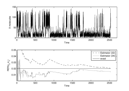
Figure 1: Upper plot: The number of $X$ molecules as a function of time. The stochastic process sequentially visits the two most probable states defined as the maxima of the PDF. Lower panel: RER as a function of time when $k_{1}A$ is perturbed by 0.05 computed using (32) (dashed line) and using (34) (grey line). In both cases, the accuracy of the numerical estimators increase as the number of samples increases.

Let denote $\theta=[k_{1}A,k_{2},k_{3}B,k_{4}]^{T}$, then the numerical estimator for RER as well as for FIM for the Schlögl model is given by (32) and (33), respectively. The upper panel of Fig. 1 shows the number of $X$ molecules in the course of time. The number of jumps of this process are $10^{6}$ while the initial value $X_{0}=100$ is slightly above the minimum of the second well. The lower panel of Fig. 1 shows the numerical RER (dashed line) as a function of time when only $k_{1}A$ is perturbed by $0.05$ (i.e., perturbation is $\epsilon=0.05e_{1}$) as well as the exact RER computed from (18). For comparison purposes, we also plot the RER estimator (34). Obviously, as simulation time is increased both numerical RER estimators converge to the exact value even though the estimator (34) needs more samples to converge (i.e., its variance is larger). Notice that enough transitions between the two steady states are necessary in order to obtain robust results. Fig. 2 depicts the exact RER (circles), the numerically-computed RER (stars) as well the FIM-based RER (squares). The directions $\pm\epsilon_{0}e_{k},\ k=1,...,4$ where $\epsilon_{0}$ is set to $0.05$ while $e_{k}$ are the typical orthonormal unit vectors are considered. These directions correspond to the perturbation of just one of the model’s parameters. The number of jumps of this simulation is $5\cdot 10^{6}$ while the initial value is again $X_{0}=100$. The numerically-computed RERs have similar values with the exact ones as Fig. 2 demonstrates. The computed RERs imply that the most sensitive parameter is $k_{2}$ (corresponds to $\pm e_{2}$) while the least sensitive parameter is $k_{3}B$ (corresponds to $\pm e_{3}$). Another important feature of the proposed sensitivity method is that the RERs for all the different parameter perturbations are computed from a single simulation run of the unperturbed process. Thus, for each direction, the only additional computational cost is the calculation of the perturbed rates of the process. Notice also that RER gives different values between a direction and its opposite resulting in assigning different sensitivities while FIM-based RER cannot distinguish between the two opposite directions since it is a second-order (quadratic) approximation.

Figure 2: Exact (circles), numerical (stars) and FIM-based (squares) RER for various directions. $k_{2}$ is the most sensitive parameter followed by $k_{1}A$ while the least sensitive parameters are $k_{4}$ and $k_{3}B$.

We further validate the inference capabilities of RER by illustrating the actual stationary distribution of the perturbed processes. It is expected that the most/least sensitive parameters of the path distribution should be strongly related with the most/least sensitive parameters of the stationary distribution. Indeed, the upper panel of Fig. 3 presents the stationary distributions of the unperturbed process (solid line) as well the perturbed stationary distribution of the most (dashed line) and least (dotted line) sensitive parameters. The perturbation of the most sensitive parameter results in the largest change of the stationary distribution while the smallest change is observed when the least sensitive parameter is perturbed. Moreover, FIM can be used for the computation not only of the most sensitive parameter but also for the computation of the most sensitive direction in general. Indeed, the most sensitive direction can be found by performing eigenvalue analysis to the FIM. The eigenvector with the highest eigenvalue defines the most sensitive direction. In our setup, the most sensitive direction is $\epsilon_{\max}=[0,0.978,0,0.207]$. The prominent parameter of the most sensitive direction is $k_{2}$ which is not a surprise since, from Fig. 2, $k_{2}$ is the most sensitive parameter. The lower panel of Fig. 3 depicts the stationary distribution of the most sensitive parameter (i.e., $k_{2}$ or $-\epsilon_{0}e_{2}$) (dashed line) and the most sensitive direction (i.e., $\epsilon_{0}\epsilon_{\max}$) (dotted line). It is evident that the stationary distribution of the most sensitive direction is further away from the unperturbed stationary distribution compared to the stationary distribution of the most sensitive parameter.

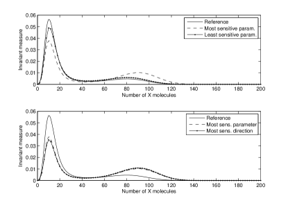
Figure 3: Upper plot: The stationary distributions for the unperturbed process (solid line), the most sensitive parameter $k_{2}$ (dashed line) and the least sensitive paramter $k_{3}B$ (dotted line). Lower plot: The stationary distributions for the unperturbed process (solid line), the most sensitive parameter $k_{2}$ (dashed line) and the most sensitive direction $\epsilon_{\max}$ (dotted line).

V.3 Reversible and non-reversible Langevin Processes

The second example we consider is a particle model with interactions which have been applied and studied primarily in molecular dynamics Rapaport (1995); Schlick (2002); Frenkel and Smit (2002); Lelievre et al. (2010) but also in biology (for instance, in swarming Ebeling and Schimansky-Geier (2008)), etc. In molecular dynamics, the Langevin dynamics is typically a Hamiltonian system coupled with a thermostat (i.e., noise). A Langevin process is defined by the SDE system

$$dq_{t}=\frac{1}{m}p_{t}dt$$ (36)

$$dp_{t}=-{\bf F}(q_{t})dt-\frac{\gamma}{m}p_{t}dt+\sigma dB_{t}$$

where $q_{t}\in\mathbb{R}^{dN}$ is the position vector of the $N$ particles in $d$ dimensions, $p_{t}\in\mathbb{R}^{dN}$ is the momentum vector of the particles, $m$ is the mass of the particles, $\bf F$ is a driving force, $\gamma$ is the friction factor, $\sigma$ is the diffusion factor and $B_{t}$ is a $dN$-dimensional Brownian motion. The first equation which describes the evolution of the position of the particles is deterministic thus the overall SDE system is degenerate. In the zero-mass limit or the infinite-friction limit, Langevin process is simplified to overdamped Langevin process which is non-degenerate, however, several studies advocate the use of Langevin dynamics directly Scemama et al. (2006); Cancès et al. (2007). The proposed sensitivity analysis approach is widely applicable to SDE systems once the assumption on ergodicity is satisfied.

The vector field ${\bf F}(\cdot)$ denotes the force exerted on the system and here we assume it consists of two terms: a gradient (potential) component as in typical Langevin systems, as well as an additional non-gradient term, where the latter is assumed to be divergence-free:

$${\bf F}(q)=\nabla_{q}V(q)+\alpha G(q)\,,$$ (37)

and $\nabla_{q}\cdot G=0$. Here we consider particular examples to illustrate the applicability of the proposed sensitivity analysis methods. The gradient term in (37) models particle interactions given by

$$V(q)=\sum_{i,j<i}V_{M}(|q_{i}-q_{j}|)$$ (38)

where $V_{M}(r)$ is the three-parameter Morse potential $V_{M}(r)=D_{e}(1-e^{-a(r-r_{e})})^{2}$. The Morse potential includes a combination of short-range repulsive and long-range attractive interactions and has been extensively used in molecular simulations Kaplan (2003). The divergence-free component is taken to be a simple antisymmetric force given by

$$G_{i}(q)=q_{i+1}-q_{i-1}\ ,\ \ \ i=1,...,N\\$$ (39)

where $q_{0}=q_{N}$ and $q_{N+1}=q_{1}$.

We now return to (37) and discuss the implications of its structure. When $\alpha=0$, the Langevin process is reversible meaning that the condition of detailed balance is satisfied with respect to a known Gibbs stationary probability distribution Lelievre et al. (2010). However, knowing the stationary distribution explicitly is insufficient to carry out sensitivity analysis on the stationary dynamics which typically may include dynamic transitions between metastable states, as in the Schlögl Model discussed earlier. Furthermore, when $\alpha\neq 0$, detailed balance does not hold true in general and the stationary probability distribution of the corresponding Langevin process is not known since the system is non-reversible Lebowitz and Spohn (1999); Maes et al. (2000). Examples of forces such as (37) that include non-gradient terms and yield non-reversible Langevin equations, arise typically in driven systems, for instance in Brownian particle suspensions where particles interact with a fluid flow Sweet et al. (2011). For non-reversible systems no efficient method for sensitivity analysis has been reported in the literature, at least for the cases dealt here, namely (a) long-time, stationary dynamics (also referred to as non-equilibrium steady states (NESS) Lebowitz and Spohn (1999); Maes et al. (2000)), as well as, (b) the unknown stationary probability. Our proposed path-space RER sensitivity methods can address these challenges and is straightforwardly applicable to both reversible and non-reversible Langevin equations as we show next.

First, an explicit EM–Verlet (symplectic)–implicit EM scheme is applied for the discretization of (LABEL:Langevin:sde:cont). It is written as

$$p_{i+\frac{1}{2}} =p_{i}-{\bf F}(q_{i})\frac{\Delta t}{2}-\frac{\gamma}{m}p_{i}\frac{\Delta t}{2}+\sigma\Delta W_{i}$$ (40)

$$q_{i+1} =q_{i}+m^{-1}p_{i+\frac{1}{2}}\Delta t$$

$$p_{i+1} =p_{i+\frac{1}{2}}-{\bf F}(q_{i+1})\frac{\Delta t}{2}-\frac{\gamma}{m}p_{i+1}\frac{\Delta t}{2}+\sigma\Delta W_{i+\frac{1}{2}}$$

with $\Delta W_{i},\Delta W_{i+\frac{1}{2}}\sim{\it N}(0,\frac{\Delta t}{2}I_{dN})$ where ${\it N}$ is the multivariate normal distribution. This numerical scheme also known as BBK integrator Brunger et al. (1984); Lelievre et al. (2010) utilizes a Strang splitting. Thus, the discretized Langevin process is a Markov chain with continuous state space. Notice that the numerical scheme is non-degenerate, thus, the transition probability from state $(q,p)$ to state $(p^{\prime},q^{\prime})$ is given by

$$P(q,p,q^{\prime},p^{\prime})=P(q^{\prime}|q,p)P(p^{\prime}|q^{\prime},q,p)$$ (41)

where

$$P(q^{\prime}|q,p)=\frac{1}{Z_{0}}e^{-\frac{m^{2}}{\sigma^{2}\Delta t^{3}}\left|q^{\prime}-q+(p-{\bf F}(q)\frac{\Delta t}{2m}+p\frac{\Delta t\gamma}{2m})\Delta t\right|^{2}}$$ (42)

and

$$P(p^{\prime}|q^{\prime},q,p)=\frac{1}{Z_{1}}e^{-\frac{1}{\sigma^{2}\Delta t}\left|(1+\frac{\gamma\Delta t}{2m})p^{\prime}-(\frac{m}{\Delta t}(q^{\prime}-q)-\frac{\Delta t}{2}{\bf F}(q^{\prime}))\right|^{2}}$$ (43)

where $Z_{i},\ i=0,1$ are the respective normalization constants. Let now define the parameter vector $\theta=[D_{e},a,r_{e}]$. Then, the discretized Langevin model (LABEL:Langevin:BBK:integrator) is a discrete-time Markov process with $\mathbb{R}^{2dN}$ being the state space. The statistical estimators for RER as well as for FIM are given by (30) and (31), respectively. Notice that the estimators with larger variance were chosen because the integration of the transition probability density function w.r.t. the positions is not a trivial problem, if not intractable in high dimensions.

Table 3: Parameter values for the discretized Langevin system.

Parameters	$N$	$D_{e}$	$a$	$r_{e}$	$m$	$\gamma$	$\sigma$	$\Delta t$
Values	3	0.3	0.3	1	1	1	0.1	0.01

The upper panel of Fig. 4 depicts the numerical RER as a function of simulation time for the parameter values given in Table 3. The reversible case is considered while the sensitivity of the parameters is obtained from the directions defined by the orthonormal unit vectors multiplied with $\epsilon_{0}=0.05$. Since the initial positions and momenta where randomly chosen from a uniform distribution an initial out-of-equilibrium time regime can be seen in the Figure (up to time $t_{0}=100$). Moreover, the variance of RER as an observable is rather large which can be explained by the small number of particles. Systems with more particles are expected to converge faster due to averaging effects. The lower panel of Fig. 4 depicts the RER at final time $t=10^{4}$ with an initial equilibration time $t_{0}=100$ where the numerical RER is discarded. Evidently, the most sensitive parameter is $a$ followed by $D_{e}$ while the least sensitive parameter is $r_{e}$.

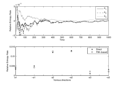
Figure 4: Upper plot: Relative entropy rate as a function of time for perturbations of $D_{e}$ (solid line), $a$ (dashed line) and of $r_{e}$ (grey line) at the reversible regime ($\alpha=0$). The variance of the numerical RER is large, necessitating more samples for accurate estimation. Lower plot: RER for various directions. The most sensitive parameter is $a$.

Utilizing our methodology the parameter sensitivity of not only the reversible regime but also of the non-reversible, $\alpha\neq 0$, regime can be explored even though the stationary probability is not known. Fig. 5 shows the level sets of the FIM matrix for the reversible case (upper plots, $\alpha=0$) and for the irreversible case (lower plots, $\alpha=0.1$). Figure suggests that the additional irreversible component results in the fact that some directions became more sensitive and some other directions became less sensitive. Further validation is obtained from the eigenvalues of the FIM which are $7.30,0.592,0.015$ for the reversible case while the eigenvalues for the irreversible case are $13.90,0.302,0.074$. Finally, FIM can be very useful in various ways for the quantification of sensitivity analysis. For instance, the determinant of FIM which in optimal experiment design is called A-optimality can be used as a measure of parameter identification Rothenberg (1971); Emery and Nenarokomov (1998); Komorowski et al. (2011). In our particular example, the determinants are $0.065$ and $0.313$ for the reversible and irreversible cases, respectively. This result asserts that in the non-reversible case $\alpha\neq 0$ in (37), the divergence-free component improves the ability of any estimator of the potential’s parameters.

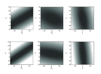
Figure 5: Upper plots: Level sets (or neutral spaces) for the reversible case ($\alpha=0$). Lower plots: Level sets for the irreversible case ($\alpha=0.1$).

V.4 Spatially extended Kinetic Monte Carlo models

The applicability of the proposed sensitivity method is further demonstrated in spatially extended systems which exhibit complex spatio-temporal morphologies such as islands, spirals, rings, etc. at mesoscale length scales. Among the various surface mechanisms such as adsorption, desorption, diffusion, etc. we focus on $CO$ oxidation which is a prototypical example for molecular-level reaction-diffusion mechanism between adsorbates on a catalytic surface. A simplified $CO$ oxidization model without diffusion known as the Ziff-Gulari-Barshad (ZGB) model Ziff et al. (1986) is considered. Despite being an idealized model, the ZGB model incorporates the basic mechanisms for the dynamics of adsorbate species during $CO$ oxidation on catalytic surfaces, namely, single site updates (adsorption/desorption) and multisite reactions (two neighboring sties being involved). Due to the reactions between species, the ZGB model is non-reversible and its stationary distribution is unknown. Nevertheless, our sensitivity analysis methodology is capable of quantify the parameter sensitivities utilizing only the rates of the process which are provided in Table 4. The spins of the two dimensional lattice $\Lambda_{N}$ with $N$ lattice sites take values $\sigma(j)=0$ denoting a vacant site $j\in\Lambda_{N}$, $\sigma(j)=-1$ for a $CO$ molecule at site $j$ and $\sigma(j)=1$ for an $O$ molecule. Depending on the local configuration of site $j$ as well as of the nearest neighbors, the events with the respective rates provided in Table 4 are executed.

Table 4: The rate of the $k$th event of the $j$th site given that the current configuration is $\sigma$ is denoted by $c_{k}(j;\sigma)$ where n.n. stands for nearest neighbors.

Event	Reaction	Rate
1	$\emptyset\rightarrow CO$	$(1-\sigma(j)^{2})k_{1}$
2	$\emptyset\rightarrow O_{2}$	$(1-\sigma(j)^{2})(1-k_{1})\frac{\#\text{vacant n.n.}}{\text{total n.n.}}$
3	$CO+O\rightarrow CO_{2}+\text{des.}$	$\frac{1}{2}\sigma(j)(1+\sigma(j))k_{2}\frac{\#O\text{ n.n.}}{\text{total n.n.}}$
4	$O+CO\rightarrow CO_{2}+\text{des.}$	$\frac{1}{2}\sigma(j)(\sigma(j)-1)k_{2}\frac{\#CO\text{ n.n.}}{\text{total n.n.}}$

The ZGB model is a high-dimensional CTMC which here is simulated utilizing the stochastic simulation algorithm Gillespie (1976). For each step of the simulation, the rates of the process for all sites of the lattice are needed. Interestingly, in order to perform our sensitivity analysis to the system parameters, only the rates are incorporated. Indeed, denoting by $\theta=[k_{1},k_{2}]$ the parameter vector, then the statistical estimators of RER as well as of FIM for the ZGB model are given by (32) and (33), respectively. Nevertheless, we explicitly provide the numerical RER estimator for convenience:

$$\bar{\mathcal{H}}_{1}^{(n)}=\frac{1}{T}\sum_{i=0}^{n-1} \Delta\tau_{i}\Big{[}\sum_{j\in\Lambda_{N}}\sum_{k=1}^{4}c_{k}^{\theta}(j;\sigma_{i})\log\frac{c_{k}^{\theta}(j;\sigma_{i})}{c_{k}^{\theta+\epsilon}(j;\sigma_{i})}$$ (44)

$$+\lambda^{\theta+\epsilon}(\sigma_{i})-\lambda^{\theta}(\sigma_{i})\Big{]}$$

where $c_{k}^{\theta}(j;\sigma)$ is the $k$th event of lattice site $j$ when the lattice configuration is $\sigma$ while $\lambda^{\theta}(\sigma)=\sum_{j\in\Lambda_{N}}\sum_{k=1}^{4}c_{k}^{\theta}(j;\sigma)$ is the total rate of the process at state $\sigma$.

The upper panel of Fig. 6 depicts the RER as a function of simulation time when $k_{1}=0.35$ is perturbed by $\epsilon_{0}=0.02$ (solid line) and when $k_{2}=0.85$ is perturbed by the same amount. It is evident that after an initial burning time, RER converges fast to a limit value implying that the variance of RER as an observable is small. This can be explained by the fact that at each step of the simulation, (44) averages the over the entire lattice in order to compute the instantaneous RER. The lower panel of Fig. 6 depicts the RER at final time $t=100$ with an initial equilibration time $t_{0}=10$ where the instantaneous RER is discarded. Obviously, the most sensitive parameter is $k_{1}$ which is related with the adsorption mechanism while the least sensitive is $k_{2}$. In order to further validate our findings, we plot the lattice configuration when either $k_{1}$ or $k_{2}$ is perturbed by $\epsilon_{0}=0.02$. Fig. 7 depicts the configuration of the unperturbed system as well as the configurations when one of the two model parameters are perturbed. Evidently, the configuration when the most sensitive parameter (i.e., $k_{1}$) is perturbed is less similar to the unperturbed configuration compared to the configuration when the least sensitive parameter (i.e., $k_{2}$) is perturbed.

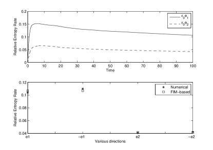
Figure 6: Upper plot: Relative entropy rate as a function of time for perturbations of both $k_{1}$ (solid line) and of $k_{2}$ (dashed line). An equilibration time until the process reach its metastable regime is evident. Lower plot: RER for various directions. The most sensitive parameter is $k_{1}$.

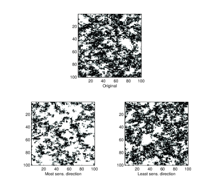
Figure 7: Configurations obtained by $\epsilon_{0}$-perturbations of the most and least sensitive parameters. The comparison with the reference configuration reveals the differences between the most and least sensitive perturbation parameters.

Thus far, we have performed local sensitivity analysis meaning that we were concentrated around a single point of the parameter space. Even though various global sensitivity analysis approaches have been derived based on variance Chan et al. (1997); Saltelli et al. (2008) or on mutual information N. Lüdtke and S. Panzeri and M. Brown and D. S. Broomhead and J. Knowles and M. A. Montemurro and D. B. Kell (2008), here, we present a demonstration of global sensitivity analysis based on a phase diagram of the most and least sensitive directions. Indeed, any direction can be seen as a vector field and a phase diagram of a subset of the parameter regime can be visualized. Fig. 8 depicts the most (solid) and least (dashed) sensitive directions which correspond to the stronger and weaker eigenvalues of the FIM, respectively. Notice that the most/least sensitive directions are parallel to the axes which asserts that the FIM is diagonal. This can be explained by the fact that the parameters of the model $k_{1}$ and $k_{2}$ affect different rates in a decoupled fashion (check Table 4).

Finally, we note that even though we have considered a spatial KMC model with few parameters to assess their sensitivity, our emphasis is primarily on (a) the high dimensionality of the process, and (b) the non-reversibility of the process without prior knowledge of the stationary probability distribution. For such complex systems there appears to be no previous systematic work in the literature on sensitivity analysis.

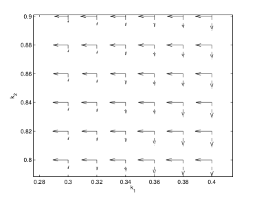
Figure 8: Vector field with the most (solid arrows) and least (dashed arrows) sensitive directions computed from eigenvalue analysis of FIM. The length of the arrows is proportional to the corresponding eigenvalue.

VI Conclusions

Here we proposed a novel method for sensitivity analysis of complex stochastic dynamics, based on the concept of Relative Entropy Rate between two stochastic processes. The method is computationally feasible at the stationary regime and involves the calculation of suitable observables in path space for the Relative Entropy Rate and the corresponding Fisher Information Matrix. The stationary regime is crucial for stochastic dynamics and can allow us to address the sensitivity analysis of complex systems, including examples of processes with complex landscapes that exhibit metastability and strong intermittency, non-reversible systems from a statistical mechanics perspective, and high-dimensional, spatially distributed models. Our proposed methods bypass these challenges relying on the direct Monte Carlo simulation of rigorously derived observables for the Relative Entropy Rate and Fisher Information in path space rather than on the stationary probability distribution itself. The knowledge of the Fisher Information Matrix provides a gradient-free method for sensitivity analysis, as well as allows to address questions of parameter identifiability and optimal experiment design in complex stochastic dynamics.

Although the proposed methods are widely applicable to many stochastic models, we demonstrated their capabilities by focusing on two classes of problems. First, on Langevin particle systems with either reversible (gradient) or non-reversible (non-gradient) forcing, highlighting the ability of the method to carry out sensitivity analysis in non-equilibrium systems; second, on spatially extended Kinetic Monte Carlo models, showing that the method can handle high-dimensional problems. In fact, we showed that the proposed approach to sensitivity analysis is suitable for non-equilibrium systems, where the structure of the stationary PDF is unknown and is typically non-Gaussian. Finally, the sensitivity estimators can be easily embedded in any available molecular simulation methods such as Kinetic Monte Carlo or Langevin solvers.

Appendix A Sensitivity analysis on the logarithmic scale

In many applications, the model parameters differ by orders of magnitude and the only meaningful option in order to study sensitivity analysis is to perform relative parameter perturbations. This is done by perturbing the logarithm of the model parameters instead of the parameters itself. Thus, utilizing the chain rule for $\nabla_{\log\theta}f(\theta)=\nabla_{\theta}f(\theta).\nabla_{\log\theta}\theta=\theta.\nabla_{\theta}f(\theta)$ where ‘.’ means element by element multiplication, the logarithmic-scale Fisher information matrix has elements:

$$\big{(}\mathbf{F_{\mathcal{H}}}({Q^{\log\theta}})\big{)}_{i,j}=\theta_{i}\theta_{j}\big{(}\mathbf{F_{\mathcal{H}}}({Q^{\theta}})\big{)}_{i,j}\ ,\ \ \ \ i,j=1,...,k\ .$$ (45)

Similarly, the logarithmic perturbation for the RER is performed by utilizing the perturbation vector $\theta.\epsilon$ instead of $\epsilon$. Notice that (7) continuous to be valid for the logarithmic scale. Indeed, it holds that

$$\mathcal{H}\left({{Q^{\theta}}}{\,|\,}{{Q^{\theta(1+\epsilon)}}}\right)=\frac{1}{2}(\theta.\epsilon)^{T}\mathbf{F_{\mathcal{H}}}({Q^{\log\theta}})(\theta.\epsilon)+O(|\theta.\epsilon|^{3})\ .$$ (46)

References

- Gunawan et al. (2005) R. Gunawan, Y. Cao, L. Petzold, and F. J. D. III, “Sensitivity analysis of discrete stochastic systems,” Biophysical Journal, 88, 2530–2540 (2005).
- Nakayama et al. (1994) M. Nakayama, A. Goyal, and P. W. Glynn, “Likelihood ratio sensitivity analysis for Markovian models of highly dependable systems,” Stochastic Models, 10, 701–717 (1994).
- Plyasunov and Arkin (2007) S. Plyasunov and A. P. Arkin, “Efficient stochastic sensitivity analysis of discrete event systems,” J. Comp. Phys., 221, 724–738 (2007).
- Kim et al. (2007) D. Kim, B. Debusschere, and H. Najm, “Spectral methods for parametric sensitivity in stochastic dynamical systems,” Biophysical Journal, 92, 379–393 (2007).
- Rathinam et al. (2010) M. Rathinam, P. W. Sheppard, and M. Khammash, “Efficient computation of parameter sensitivities of discrete stochastic chemical reaction networks,” J. Chem. Phys., 132, 034103–(1–13) (2010).
- Wu et al. (2012) C. Wu, D. J. Schmidt, C. Wolverton, and W. F. Schneider, “Accurate coverage-dependence incorporated into first-principles kinetic models: Catalytic NO oxidation on Pt (111),” J. Catalysis, 286, 88–94 (2012).
- Liu et al. (2006) H. Liu, W. Chen, and A. Sudjianto, “Relative entropy based method for probabilistic sensitivity analysis in engineering design,” J. Mechanical Design, 128, 326–336 (2006).
- N. Lüdtke and S. Panzeri and M. Brown and D. S. Broomhead and J. Knowles and M. A. Montemurro and D. B. Kell (2008) N. Lüdtke and S. Panzeri and M. Brown and D. S. Broomhead and J. Knowles and M. A. Montemurro and D. B. Kell, “Information-theoretic sensitivity analysis: a general method for credit assignment in complex networks,” J. R. Soc. Interface, 5, 223–235 (2008).
- Majda and Gershgorin (2010) A. J. Majda and B. Gershgorin, “Quantifying uncertainty in climate change science through empirical information theory,” Proc. of the National Academy of Sciences, 107, 14958–14963 (2010).
- Majda and Gershgorin (2011) A. J. Majda and B. Gershgorin, “Improving model fidelity and sensitivity for complex systems through empirical information theory,” Proc. of the National Academy of Sciences, 108, 10044–10049 (2011).
- Komorowski et al. (2011) M. Komorowski, M. J. Costa, D. A. Rand, and M. P. H. Stumpf, “Sensitivity, robustness, and identifiability in stochastic chemical kinetics models,” Proc. Natl. Acad. Sci. USA, 108, 8645–8650 (2011).
- Doering et al. (2007) C. R. Doering, K. V. Sargsyan, L. M. Sander, and E. Vanden-Eijnden, “Asymptotics of rare events in birth–death processes bypassing the exact solutions,” Journal of Physics: Condensed Matter, 19, 065145–(1–12) (2007).
- Hanggi et al. (1984) P. Hanggi, H. Grabert, P. Talkner, and H. Thomas, “Bistable systems: Master equation versus Fokker-Planck modeling,” Phys. Rev. A, 29, 371–378 (1984).
- Katsoulakis et al. (2006) M. A. Katsoulakis, A. J. Majda, and A. Sopasakis, “Intermittency, metastability and coarse graining for coupled deterministic-stochastic lattice systems,” Nonlinearity, 19, 1021–1047 (2006).
- Liggett (1985) T. Liggett, Interacting particle systems (Springer - Berlin, 1985).
- Chatterjee and Vlachos (2007) A. Chatterjee and D. G. Vlachos, “An overview of spatial microscopic and accelerated kinetic Monte Carlo methods for materials’ simulation,” J. Computer-Aided Materials Design, 14, 253–308 (2007).
- Cover and Thomas (1991) T. M. Cover and J. A. Thomas, Elements of Information Theory (Wiley Series in Telecommunications, 1991).
- Katsoulakis and Trashorras (2006) M. A. Katsoulakis and J. Trashorras, “Information loss in coarse-graining of stochastic particle dynamics,” J. Stat. Phys., 122, 115–135 (2006).
- Katsoulakis et al. (2007) M. A. Katsoulakis, L. Rey-Bellet, P. Plecháč, and D. K. Tsagkarogiannis, “Coarse-graining schemes and a posteriori error estimates for stochastic lattice systems,” ESAIM-Math. Model. Num. Analysis, 41, 627–660 (2007).
- Arnst and Ghanem (2008) M. Arnst and R. Ghanem, “Probabilistic equivalence and stochastic model reduction in multiscale analysis,” Comp. methods in applied mech. and eng., 197, 3584–3592 (2008).
- Kipnis and Landim (1999) C. Kipnis and C. Landim, Scaling Limits of Interacting Particle Systems (Springer-Verlag, 1999).
- Maes et al. (2000) C. Maes, F. Redig, and A. V. Moffaert, “On the definition of entropy production, via examples,” J. Math. Phys., 41, 1528–1553 (2000).
- Abramov et al. (2005) R. V. Abramov, M. J. Grote, and A. J. Majda, Information Theory and Stochastics for Multiscale Nonlinear Systems (CRM Monograph Series, 2005).
- Rao et al. (2009) S. K. Rao, R. Imam, K. Ramanathan, and S. Pushpavanam, “Sensitivity Analysis and Kinetic Parameter Estimation in a Three Way Catalytic Converter,” Industrial & Engineering Chemistry Research, 48, 3779–3790 (2009).
- Braatz et al. (2006) R. Braatz, R. Alkire, E. Seebauer, E. Rusli, R. Gunawan, T. Drews, X. Li, and Y. He, “Perspectives on the design and control of multiscale systems,” J. Proc. Control, 16, 193–204 (2006).
- Rothenberg (1971) T. Rothenberg, “Identification in parametric models,” ECONOMETRICA, 39, 577–0591 (1971).
- Emery and Nenarokomov (1998) A. F. Emery and A. V. Nenarokomov, “Optimal experiment design,” Measurement Science & Technology, 9, 864–876 (1998).
- Prasad et al. (2010) V. Prasad, A. M. Karim, Z. Ulissi, M. Zagrobelny, and D. G. Vlachos, “High throughput multiscale modeling for design of experiments, catalysts, and reactors: Application to hydrogen production from ammonia,” Chem. Eng. Sci., 65, 240–246 (2010).
- Gillespie (2001) D. T. Gillespie, “Approximated accelerated stochastic simulation of chemically reacting systems,” J. Chem. Phys., 115, 1716–1733 (2001).
- Plimpton et al. (2009) S. Plimpton, C. Battaile, M. Chandross, L. Holm, A. Thompson, V. Tikare, G. Wagner, E. Webb, X. Zhou, C. G. Cardona, and A. Slepoy, “Crossing the Mesoscale No-Man’s Land via Parallel Kinetic Monte Carlo,” Tech. Rep. (Sandia National Laboratory, 2009).
- Plimpton and Thompson (2012) S. J. Plimpton and A. P. Thompson, “Computational aspects of many-body potentials,” MRS Bull., 37, 513–521 (2012).
- Arampatzis et al. (2012) G. Arampatzis, M. A. Katsoulakis, P. Plechac, M. Taufer, and L. Xu, “Hierarchical fractional-step approximations and parallel kinetic Monte Carlo algorithms,” J. Comp. Phys., 7795–7814 (2012).
- Hansen and Neurock (2000) E. W. Hansen and M. Neurock, “First-principles-based Monte Carlo simulation of ethylene hydrogenation kinetics on Pd,” J. Catalysis, 196, 241–252 (2000).
- Meskine et al. (2009) H. Meskine, S. Matera, M. Scheffler, K. Reuter, and H. Metiu, “Examination of the concept of degree of rate control by first-principles kinetic Monte Carlo simulations,” Surf. Science, 603(10-12), 1724–1730 (2009).
- Stamatakis et al. (2011) M. Stamatakis, Y. Chen, and D. G. Vlachos, “First-principles-based kinetic Monte Carlo simulation of the structure sensitivity of the water-gas shift reaction on Platinum surfaces,” Journal of Physical Chemistry C, 115(50), 24750–24762 (2011).
- Note (1) This Lebesgue continuity assumption is merely for simplification purposes and it can be easily generalized.
- Liptser and Shiryaev (1977) R. S. Liptser and A. N. Shiryaev, Statistics of Random Processes: I & II (Springer, 1977).
- Dumitrescu (1988) M. E. Dumitrescu, “Some informational properties of markov pure-jump processes,” C. P. Matematiky, 113, 429–434 (1988).
- Wen and Weiguo (1996) L. Wen and Y. Weiguo, “An extension of Shannon-McMillan theorem and some limit properties for nonhomogeneous Markov chains,” Stochastic Processes and their Applications, 61, 129–145 (1996).
- Limnios and Oprisan (2001) N. Limnios and G. Oprisan, Semi-Markov Processes and Reliability (Springer, 2001).
- Lutz and Kiremidjian (1993) K. A. Lutz and A. S. Kiremidjian, “A generalized semi-Markov process for modeling spatially and temporally dependent earthquakes,” Tech. Rep. (The J. A. Blume Earthquake Engineering Center, 1993).
- Janssen and Manca (2006) J. Janssen and R. Manca, Applied Semi-Markov Processes (Springer, 2006).
- Girardin and Limnios (2003) V. Girardin and N. Limnios, “On the entropy for semi-Markov processes,” J. Appl. Probab., 40, 1060–1068 (2003).
- Gillespie (1976) D. T. Gillespie, “A general method for numerically simulating the stochastic time evolution of coupled chemical reactions,” J. Comp. Phys., 22, 403–434 (1976).
- Schlögl (1972) F. Schlögl, “Chemical reaction models for nonequilibrium phase transition,” Z. Physik, 253, 147–161 (1972).
- Vellela and Qian (2009) M. Vellela and H. Qian, “Stochastic dynamics and non-equilibrium thermodynamics of a bistable chemical system: the Schlögl model revisited,” J. R. Soc. Interface, 6, 925–940 (2009).
- Gardiner (1985) C. Gardiner, Handbook of Stochastic Methods: for Physics, Chemistry and the Natural Sciences (Springer, 1985).
- Degasperi and Gilmore (2008) A. Degasperi and S. Gilmore, “Sensitivity analysis of stochastic models of bistable biochemical reactions,” SFM 2008, 1–20 (2008).
- Rapaport (1995) D. C. Rapaport, The Art of Molecular Dynamics Simulations (Cambridge University Press, 1995).
- Schlick (2002) T. Schlick, Molecular Modeling and Simulation (Springer, 2002).
- Frenkel and Smit (2002) D. Frenkel and B. Smit, Understanding Molecular Simulation, From Algorithms to Applications (Academic Press, 2002).
- Lelievre et al. (2010) T. Lelievre, M. Rousset, and G. Stoltz, Free energy computations: a mathematical perspective (Imperial College Press, 2010).
- Ebeling and Schimansky-Geier (2008) W. Ebeling and L. Schimansky-Geier, “Swarm dynamics, attractors and bifurcations of active Brownian motion,” Eur. Phys. J. Special Topics, 157, 17–31 (2008).
- Scemama et al. (2006) A. Scemama, T. Lelièvre, G. Stoltz, E. Cancès, and M. Caffarel, “An efficient sampling algorithm for variational Monte-Carlo,” J. Chem. Phys., 125, 114105(1–9) (2006).
- Cancès et al. (2007) E. Cancès, F. Legoll, and G. Stoltz, “Theoretical and numerical comparison of sampling methods for molecular dynamics,” Math. Model. Numer. Anal., 41, 351–390 (2007).
- Kaplan (2003) I. Kaplan, Handbook of Molecular Physics and Quantum Chemistry (Wiley, 2003).
- Lebowitz and Spohn (1999) J. L. Lebowitz and H. Spohn, “A Gallavotti-Cohen type symmetry in the large deviation functional for stochastic dynamics,” J. Stat. Phys., 95, 333–365 (1999).
- Sweet et al. (2011) C. R. Sweet, S. Chatterjee, Z. Xu, K. Bisordi, E. D. Rosen, and M. Alber, “Modelling platelet-blood flow interaction using the subcellular element Langevin method,” J. Royal Society Interface, 8, 1760–1771 (2011).
- Brunger et al. (1984) A. Brunger, C. B. Brooks, and M. Karplus, “Stochastic boundary conditions for molecular dynamics simulations of ST2 water,” Chem. Phys. Lett., 105, 495–500 (1984).
- Ziff et al. (1986) R. M. Ziff, E. Gulari, and Y. Barshad, “Kinetic phase transitions in an irreversible surface-reaction model,” Phys. Rev. Lett., 56, 2553 (1986).
- Chan et al. (1997) K. Chan, A. Saltelli, and S. Tarantola, “Sensitivity analysis of model output: variance-based methods make the difference,” Proc. of the 29th conf. on Winter simulation, 261–268 (1997).
- Saltelli et al. (2008) A. Saltelli, M. Ratto, T. Andres, F. Campolongo, J. Cariboni, D. Gatelli, M. Saisana, and S. Tarantola, Global Sensitivity Analysis. The Primer (Wiley, 2008).