Resonant quantum kicked rotor with two internal levels

Abstract

We develop a system consisting of a quantum kicked rotor with an additional degree of freedom. This models a single two-level atom with internal ground and excited states, and it is characterized by its quantum resonances with ballistic spreading and by the entanglement between the internal and momentum degrees of freedom. These behaviors establish an equivalence between our model and the usual quantum walk on the line.

I Introduction

Advances in technology during the last decades have made it possible to obtain samples of atoms at temperatures in the $nK$ range Cohen (optical molasses) using resonant or quasiresonant exchanges of momentum and energy between atoms and laser light. The experimental progress that has allowed to construct and preserve quantum states has also opened the possibility of building quantum computing devices Dur ; Sanders ; Du ; Berman and has led the scientific community to think that quantum computers could be a reality in the near future. This progress has been accompanied with the development of the interdisciplinary fields of quantum computation and quantum information. In this scientific framework, the study of simple quantum systems such as the quantum kicked rotor (QKR) Casati0 ; Izrailev and the quantum walk (QW) Kempe may be useful to understand the quantum behavior of atoms in optical molasses.

The QKR is considered as the paradigm of periodically driven systems in the study of chaos at the quantum level Casati0 . This system shows behaviors without classical equivalent, such as quantum resonance and dynamical localization, which have posed interesting challenges both in theoretical and experimental Nielssen terms. The occurrence of quantum resonance or dynamical localization depends on whether the period of the kick $T$ is a rational or irrational multiple of $4\pi$. For rational multiples, the behavior of the system is resonant while for irrational multiples the average energy of the system grows in a diffusive manner for a short time and then the diffusion stops and localization appears. From a theoretical point of view the two types of values of $T$ determine the spectral properties of the Hamiltonian. For irrational multiples the energy spectrum is purely discrete and for rational multiples it contains a continuous part. Both resonance and localization can be seen as interference phenomena, the first being a constructive interference effect and the second a destructive one. The QKR has been used as a theoretical model for several experimental situations dealing with atomic traps Moore0 ; Kanem ; Chaudhury ; Moore1 ; Robinson0 ; Robinson1 ; Bharucha ; Oskay and is a matter of permanent attention Schomerus0 ; Schomerus1 ; alejo ; alejo0 ; alejo1 ; alejo2 ; alejo3 ; alejo4 ; alejo5 .

The quantum walk has been introduced Aharonov ; Meyer ; Watrous ; Ambainis ; Kempe ; Kendon1 ; Kendon2 ; Konno ; Salvador as a natural generalization of the classical random walk in relation with quantum computation and quantum information processing. In both cases there is a walker and a coin; at every time step the coin is tossed and the walker moves depending on the toss output. In the classical random walk the walker moves to the right or to the left, while in the QW coherent superpositions right/left and head/tail happen. This feature endows the QW with outstanding properties, such as the linear growth with time of the standard deviation of the position of an initially localized walker. as compared with its classical counterpart, where this growth goes as $t^{1/2}$. This has strong implications in terms of the realization of algorithms based on QWs and is one of the reasons why they have received so much attention. It has been suggested Childs that the QW can be used for universal quantum computation. Some possible experimental implementations of the QW have been proposed by a number of authors Dur ; Travaglione ; Sanders ; Knight ; Bouwmeester ; Do ; Chandrashekar . In particular the development of techniques to trap samples of atoms using resonant exchanges of momentum and energy between atoms and laser light may also provide a realistic frame to implement quantum computers Cirac .

A parallelism between the behavior of the QKR and a generalized form of the QW was developed in Refs. alejo0 ; alejo1 showing that these models have similar dynamics. In those papers, the modified QW was mapped into a one-dimensional Anderson model Anderson , as had been previously done for the QKR Grempel . In the present paper, following the work of Saunders $et$ $al.$ Saunders1 ; Saunders2 we propose a modification of the QKR. We study some properties of this new version of the QKR and establish a novel equivalence between this new QKR and the QW. Essentially, the new QKR has an additional degree of freedom which describes the internal ground and excited states of a two-level atom. We call this new system the two-level quantum kicked rotor (2L-QKR). In this system the internal atomic levels are coupled with the momentum of the particle. This coupling produces an entanglement between the internal degrees of freedom and the momentum of the system.

The rest of the paper is organized as follows, in the next section we present the 2L-QKR system. In the third section we obtain the time evolution of the moments. In the fourth section the entanglement between the internal degrees of freedom and momentum is studied. In the last section some conclusions are drawn.

II Two-level quantum kicked rotor

We consider a Hamiltonian that describes a single two-level atom of mass $M$ with center-of-mass momentum described by the operator $\widehat{P}$. Its internal ground state is denoted by the vector $|g\rangle$ and its excited state by the vector $|e\rangle$. The internal atomic levels are coupled by two equal-frequency laser traveling waves with a controllable phase difference. Following Saunders1 , after a shift of the energy values, the 2L-QKR Hamiltonian can be written as

$$\widehat{H} = \frac{\widehat{P}^{2}}{2M}+\hbar\Delta|e\rangle\langle e|$$ (1)

$$+K\delta_{T}(t)\cos(k_{L}\widehat{z})(|e\rangle\langle g|+|g\rangle\langle e|).$$

Here $\Delta$ is the detuning between the laser frequency and atomic transition frequency. $K$ is proportional to the Rabbi frequency and we shall refer to it as the strength parameter.

$$\delta_{T}(t)=\sum_{n=0}^{n=\infty}\delta(t-nT)$$ (2)

is a series of periodic Dirac’s delta applied at times $t=nT$ with $n$ integer and $T$ the kick period. $\widehat{z}$ is the operator of the atom’s center of mass position. Finally, $k_{L}$ is the laser wave-vector magnitude along the $z$ direction.

Unlike the QKR, in the 2L-QKR the conjugate position and momentum operators have discrete and continuous components, i.e.

$$\widehat{z}=\frac{1}{k_{L}}(2\pi\widehat{l}+\widehat{\theta})$$ (3)

$$\widehat{P}=\hbar{k_{L}}(\widehat{k}+\widehat{\beta})$$ (4)

where the eigenvalues of $\widehat{l}$ and $\widehat{k}$ are integers and the eigenvalues of $\widehat{\theta}\in[-\pi,\pi)$ and the eigenvalues of the quasimomentum $\widehat{\beta}\in[-1/2,1/2)$. It is important to point out that the operator $\widehat{\beta}$ commutes with both $\widehat{k}$ and $\widehat{\theta}$. Using Eqs.(3,4) to substitute $\widehat{z}$ and $\widehat{P}$ in Eq.(1) yields

$$\widehat{H} = \frac{\left[\hbar{k_{L}}(\widehat{k}+\widehat{\beta})\right]^{2}}{2M}+\hbar\Delta|e\rangle\langle e|$$ (5)

$$+K\delta_{T}(t)\cos(\widehat{\theta})(|e\rangle\langle g|+|g\rangle\langle e|).$$

It must be noted that Eq.(5) does not depend on the operator $\widehat{l}$ and therefore $\widehat{\beta}$ is a preserved quantity. Then if the initial condition belongs to a subspace corresponding to a well defined eigenvalue of $\widehat{\beta}$, the dynamics is such that the system remains in said subspace and the evolution of the system will be only determined by the conjugate operators $\widehat{\theta}$ and $\widehat{k}$. Therefore we may restrict ourselves to the study of the evolution constrained to a subspace corresponding to a given eigenvalue of $\beta$. In this case the composite Hilbert space for the Hamiltonian Eq.(5) is the tensor product $\mathcal{H}_{s}\otimes\mathcal{H}_{c}$. $\mathcal{H}_{s}$ is the Hilbert space associated to the discrete momentum on the line and it is spanned by the set $\{|k\rangle\}$. $\mathcal{H}_{c}$ is the chirality (or coin) Hilbert space spanned by two orthogonal vectors $\{|g\rangle,|e\rangle\}$. In this composite space the system evolves, at discrete time steps $t\in\mathbb{N}$, along a one-dimensional lattice of sites $k\in\mathbb{Z}$. The direction of motion depends on the state of the chirality. Taking this into account it is clear that the Hilbert space of the 2L-QKR (with the preceding restriction) is identical to that of the usual QW on the line.

The evolution of the system is governed by the Hamiltonian given by Eq.(5), so that, as is the case for the usual QKR, the unitary time evolution operator for one temporal period $T$ can be written as the application of two operators, one representing the unitary operator due to the kick and another being the unitary operator of the free evolution Saunders1

$$\widehat{U}=e^{-i\left[\hbar\Delta|e\rangle\langle e|+\tau(\widehat{k}+\widehat{\beta})^{2}\right]}e^{i\kappa cos{\widehat{\theta}}\sigma_{x}}$$ (6)

where $\sigma_{x}$ is the Pauli matrix in the $x$ direction,

$$\tau=\frac{k_{L}^{2}\hbar}{2M}T,$$ (7)

and

$$\kappa=\frac{K}{\hbar}.$$ (8)

The unit operator Eq.(6) in the momentum representation and in the chirality base $\left\{|e\rangle,|g\rangle\right\}$ has the following shape

$$U(\beta)_{jk} = f_{jk}(\beta,\kappa,\tau)$$ (12)

$$.\left(\begin{array}[]{cc}e^{-i\widetilde{\Delta}}\delta_{k-j\text{ }2l}&e^{-i\widetilde{\Delta}}\delta_{k-j\text{ }2l+1}\\ \delta_{k-j\text{ }2l+1}&\delta_{k-j\text{ }2l}\end{array}\right),$$

where

$$f_{jk}(\beta,\kappa,\tau)=i^{k-j}J_{k-j}\left(\kappa\right)e^{-i(j+\beta)^{2}\tau},$$ (13)

$\delta_{kj}$ is the Kronecker delta, $l$ is an integer number and

$$\widetilde{\Delta}=T\Delta=\frac{2M}{k_{L}^{2}\hbar}\tau\Delta.$$ (14)

The wave-vector in the momentum representation can be expressed as the spinor

$$|\Psi(t)\rangle \equiv \left(\begin{array}[]{c}|\Psi^{e}(t)\rangle\\ |\Psi^{g}(t)\rangle\end{array}\right)$$ (17)

$$= \sum_{k=-\infty}^{\infty}\int_{-\frac{1}{2}}^{\frac{1}{2}}\left(\begin{array}[]{c}a_{k+\beta^{\prime}}(t)\\ b_{k+\beta^{\prime}}(t)\end{array}\right)\delta(\beta-\beta^{\prime})|k+\beta^{\prime}\rangle d\beta^{\prime},$$ (20)

where $\beta$ is the value of $\beta^{\prime}$ for the chosen subspace and

$$\left(\begin{array}[]{c}a_{k+\beta}(t)\\ b_{k+\beta}(t)\end{array}\right)=\left(\begin{array}[]{c}\langle{k+\beta}|\Psi^{e}(t)\rangle\\ \langle{k+\beta}|\Psi^{g}(t)\rangle\end{array}\right),$$ (21)

are the upper and lower components that correspond to the left and right chirality of the QW.

The discrete quantum map is obtained using Eqs.(12,17)

$$\left(\begin{array}[]{c}a_{k+\beta}(t+T)\\ b_{k+\beta}(t+T)\end{array}\right)=\sum_{j=-\infty}^{\infty}U(\beta)_{kj}\left(\begin{array}[]{c}a_{j+\beta}(t)\\ b_{j+\beta}(t)\end{array}\right).$$ (22)

The dynamical evolution of the system up to $t=nT$ is obtained applying the above rule Eq.(22) $n$ times.

II.1 Resonance $\tau=2\pi$ in the $\beta=0$ subspace with $\widetilde{\Delta}=2m\pi$

In this subsection we solve analytically the evolution of the system given by the map Eq.(22). We consider here the principal resonance $\tau=2\pi$ in the subspace $\beta=0$. Due to the quasimomentum conservation the value of $\beta$ does not change. Therefore the accessible momentum spectrum is discrete and from now on the theoretical development is similar to that of the usual QKR in resonance. Additionally we choose $\widetilde{\Delta}=2m\pi$ with $m$ integer in order to obtain the wave function analytically. We will show afterwards, using numerical calculation, that the qualitative behavior will be similar for arbitrary $\widetilde{\Delta}$. With these conditions the matrix of Eq.(12) only depends on $j-k$. In order to simplify the notation we define

$$U_{k_{a}k_{b}}(\kappa)=f_{k_{a}k_{b}}(0,\kappa,2\pi)\left(\begin{array}[]{cc}\delta_{k_{a}-k_{b}\text{ }2l}&\delta_{k_{a}-k_{b}\text{ }2l+1}\\ \delta_{k_{a}-k_{b}\text{ }2l+1}&\delta_{k_{a}-k_{b}\text{ }2l}\end{array}\right).$$ (23)

Using Eq.(22) the initial condition is connected with the wave function at the time $t=nT$ by the equation

$$\left(\begin{array}[]{c}a_{k_{n}}(nT)\\ b_{k_{n}}(nT)\end{array}\right) = \sum_{k_{n-1}}\sum_{k_{n-2}}\sum_{k_{n-3}}...$$ (29)

$$...\sum_{k_{2}}\sum_{k_{1}}\sum_{k_{0}}U_{k_{n}k_{n-1}}(\kappa)U_{k_{n-1}k_{n-2}}(\kappa)...$$

$$...U_{k_{2}k_{1}}(\kappa)U_{k_{1}k_{0}}(\kappa)\left(\begin{array}[]{c}a_{k_{0}}^{0}\\ b_{k_{0}}^{0}\end{array}\right),$$

where $a_{k_{0}}^{0}=a_{k_{0}}(0)$ and $b_{k_{0}}^{0}=b_{k_{0}}(0)$.

Using the relation,

$$\sum_{k_{n-1}}U_{k_{n}k_{n-1}}(\kappa_{{1}})U_{k_{n-1}k_{n-2}}(\kappa_{{2}}) = U_{k_{n}k_{n-2}}(\kappa_{{1}}+\kappa_{{2}}),$$

obtained in Appendix A, Eq.(29) is reduced to

$$\left(\begin{array}[]{c}a_{k}(nT)\\ b_{k}(nT)\end{array}\right) = \sum_{j}i^{j-k}J_{j-k}\left(n\kappa\right)\left\{\delta_{j-k\text{ }2l}\left(\begin{array}[]{c}a_{j}^{0}\\ b_{j}^{0}\end{array}\right)\right.$$ (38)

$$+\delta_{j-k\text{ }2l+1}\left.\left(\begin{array}[]{c}b_{j}^{0}\\ a_{j}^{0}\end{array}\right)\right\},\$$

where $l$ is now an arbitrary integer number.

II.2 Antiresonance $\tau=2\pi$ in the $\beta=0$ subspace with $\widetilde{\Delta}=(2m+1)\pi$

We now find the time evolution of the wave function for $\widetilde{\Delta}=(2m+1)\pi$. Eq.(12) shows that in this case the matrix $U(\beta=0)_{jk}$ satisfies the relation

$$\sum_{k_{n-1}}U_{k_{n}k_{n-1}}(\kappa)U_{k_{n-1}k_{n-2}}(\kappa)=\delta_{k_{n}\text{ }k_{n-2}}I,$$ (39)

where $I$ is the identity matrix. This last expression together with Eq.(22) imply that

$$\left(\begin{array}[]{c}a_{k}(nT)\\ b_{k}(nT)\end{array}\right) = \text{\ }\delta_{n\text{ }2l+1}\sum_{j}U_{kj}(\kappa)\left(\begin{array}[]{c}a_{j}^{0}\\ b_{j}^{0}\end{array}\right)$$ (47)

$$+\text{ \ }\delta_{n\text{ }2l}\text{ }\left(\begin{array}[]{c}a_{k}^{0}\\ b_{k}^{0}\end{array}\right).$$

Then it is clear that the 2L-QKR shows a periodic behavior when the parameters of the system take the values here considered. This behavior has no analog in the usual QKR since the parameter $\widetilde{\Delta}$ does not exist in said system. Furthermore, it is interesting to point out that this anti-resonance occurs for $\tau=2\pi$, value for which the usual QKR is in resonance and does not present periodic behavior.

III Probability distribution of momentum

The evolution of the variance, $\sigma^{2}=m_{2}-m_{1}^{2}$, of the probability distribution of momentum is a distinctive feature of the QKR in resonance. It is known that it increases quadratically in time in the quantum case, but only linearly in the classical case. In this section we study the evolution of the variance of the 2L-QKR, once again restricting ourselves to the $\beta=0$ subspace and taking $\tau=2\pi$, which corresponds to the primary resonance of the usual QKR model. We will obtain the variance from the evolution of the first and second moments, defined as $m_{1}(t)=\sum_{k}kP_{k}(t)$ and $m_{2}(t)=\sum_{k}k^{2}P_{k}(t)$ respectively, where $P_{k}(t)=|a_{k}(t)|^{2}+|b_{k}(t)|^{2}$ is the probability to find the particle with momentum $p=\hbar k_{L}k$ at time $t$.

We first consider the resonance defined by $\widetilde{\Delta}=2m\pi$. In this case we are able to calculate the first and second moments analytically using Eq.(38) and the properties of the Bessel functions (see Appendix B), obtaining:

$$m_{1}(n)=\kappa n\sum_{j=-\infty}^{\infty}\Im\left[a_{j}^{0}b_{j+1}^{0\ast}-a_{j}^{0}b_{j-1}^{0\ast}\right]+m_{1}(0)\text{,}$$ (48)

$$m_{2}(n) = \frac{(\kappa n)^{2}}{2}\left(1+\sum_{j=-\infty}^{\infty}\Re\left[a_{j}^{0}a_{j+2}^{0\ast}(0)+b_{j}^{0}b_{j+2}^{0\ast}\right]\right)$$ (49)

$$+\kappa n\sum_{j=-\infty}^{\infty}(2j+1)\Im\left[a_{j}^{0}b_{j+1}^{0\ast}+a_{j}^{0}b_{j-1}^{0\ast}\right]\text{ }$$

$$+m_{2}(0)\text{,}$$

where $\Re\left[x\right]$ and $\Im\left[x\right]$ are respectively the real part and imaginary part of $x.$ $m_{1}(0)$ and $m_{2}(0)$ are the moments at time $t=0$. These last equations show that the behavior of the variance $\sigma^{2}=m_{2}-m_{1}^{2}$ has a quadratic time dependence irrespective of the initial conditions taken.
When $\widetilde{\Delta}=(2n+1)\pi$, it was shown in the previous section that the 2L-QKR has a periodic dynamics and therefore the behavior of the statistical moments will be periodic as well.
The case when $\widetilde{\Delta}\neq 2n\pi$ is cumbersome to solve analytically, so we restrict ourselves to a numerical study. The evolution of the second statistical moment was obtained for different values of $\widetilde{\Delta}$ through numerical iterations of the map given by Eq.(22). It was found, for all the considered values of $\widetilde{\Delta}\neq 2n\pi$, that the long-time behavior of the second moment (and therefore of the variance) is quadratic after an initial transient. The duration of the initial transient depends on the initial conditions and the value of $\widetilde{\Delta}$. This features can be appreciated in Fig.(1).

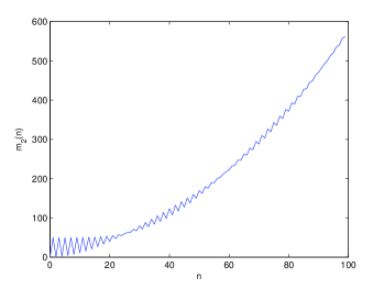
Figure 1: The dimensionless second moment for $\widetilde{\Delta}=0.97\pi$ as a function of the dimensionless time.

The figure shows the time evolution of the second moment for the initial conditions $|\Psi(0)\rangle=|k=0\rangle|g\rangle$. It can be appreciated that the second moment approaches a quadratic behavior after an oscillatory transient. It was found that the nearer the parameter $\widetilde{\Delta}$ is to $(2n+1)\pi$, the more pronounced this oscillation is.

IV Entanglement

In the context of QWs several authors Carneiro ; Abal ; Annabestani ; Omar ; Pathak ; Liu ; Venegas ; Endrejat ; Bracken ; Ellinas ; Maloyer ; alejo2010 ; alejo2012 have been investigating the relationship between the asymptotic coin-position entanglement and the initial conditions of the walk. In order to compare the model considered in this paper with the QW, we investigate the asymptotic chirality-momentum entanglement in the 2L-QKR. The unitary evolution of the 2L-QKR generates entanglement between chirality and momentum degrees of freedom. This entanglement will be characterized Carneiro ; alejo2010 by the von Neumann entropy of the reduced density operator, called entropy of entanglement. The quantum analog of the Gibbs entropy is the von Neumann entropy

$$S_{N}(\rho)=-\text{tr}(\rho\log\rho),$$ (50)

where $\rho=|\Psi(t)\rangle\left\langle\Psi(t)\right|$ is the density matrix of the quantum system. Owing to the unitary dynamics of the 2L-QKR, the system remains in a pure state, and this entropy vanishes. In spite of this chirality and momentum are entangled, and the entanglement can be quantified by the associated von Neumann entropy for the reduced density operator:

$$S=-\text{tr}(\rho_{c}\log_{2}\rho_{c}),$$ (51)

where $\rho_{c}=$tr${}_{k}(\rho)$ is the reduced density matrix that results from taking the partial trace over the momentum space. The reduced density operator can be explicitly obtained using the wave function Eq.(17) in the subspace $\beta=0$ and its normalization properties

$$\rho_{c}=\left(\begin{array}[]{cc}P_{g}(n)&Q(n)\\ Q^{\ast}(n)&P_{e}(n)\end{array}\right),$$ (52)

where

$$P_{g}(n)=\sum_{j=-\infty}^{\infty}\left|a_{k}(nT)\right|^{2}\text{,}$$ (53)

$$P_{e}(n)=\sum_{j=-\infty}^{\infty}\left|b_{k}(nT)\right|^{2}\text{,}$$ (54)

$$Q(n)=\sum_{j=-\infty}^{\infty}a_{k}(nT)b_{k}^{\ast}(nT)\text{.}$$ (55)

$P_{e}(n)$ and $P_{g}(n)$ may be interpreted as the time-dependent probabilities for the system to be in the excited and the ground states respectively. In order to investigate the entanglement dependence on the initial conditions, we consider the localized case, that is the initial state of the rotor is assumed to be sharply localized with vanishing momentum and arbitrary chirality, thus

$$\left(\begin{array}[]{c}{a_{k}(0)}\\ {b_{k}(0)}\end{array}\right)=\left(\begin{array}[]{c}\cos{\frac{\gamma}{2}}\\ \exp i\varphi\text{ }\sin{\frac{\gamma}{2}}\end{array}\right)\delta_{k0},$$ (56)

where $\gamma\in\left[0,\pi\right]$ and $\varphi\in\left[0,2\pi\right]$ define a point on the unit three-dimensional Bloch sphere. Eq.(38) takes the following form

$$\left(\begin{array}[]{c}a_{k}(nT)\\ b_{k}(nT)\end{array}\right) = i^{k}J_{k}\left(n\kappa\right)\left\{\delta_{k\text{ }2l}\left(\begin{array}[]{c}\cos{\frac{\gamma}{2}}\\ \exp i\varphi\text{ }\sin{\frac{\gamma}{2}}\end{array}\right)\right.$$ (64)

$$+\delta_{k\text{ }2l+1}\left.\left(\begin{array}[]{c}\exp i\varphi\text{ }\sin{\frac{\gamma}{2}}\\ \cos{\frac{\gamma}{2}}\end{array}\right)\right\}.$$

Substituting Eq.(64) into Eqs.(53,54,55) and using the properties of the Bessel functions, we obtain:

$$P_{g}(n)=\frac{1}{2}\left[1+J_{0}(2n\kappa)\cos\gamma\right]\text{,}$$ (65)

$$P_{e}(n)=\frac{1}{2}\left[1-J_{0}(2n\kappa)\cos\gamma\right]\text{,}$$ (66)

$$Q(n)=\frac{\sin\gamma}{2}\left[\cos\varphi-i\sin\varphi J_{0}(2n\kappa)\right]\text{.}$$ (67)

The eigenvalues of the density operator $\rho_{c}$, Eq.(52), as a function of $P_{g}(n)$, $P_{e}(n)$ and $Q(n)$ is

$$\lambda_{\pm}=\frac{1}{2}\left[1\pm\sqrt{1-4\left(P_{g}(n)\,P_{e}(n)-\left|Q(n)\right|^{2}\right)}\right],$$ (68)

and the reduced entropy as a function of these eigenvalues is

$$S(n)=-\lambda_{+}\log_{2}\lambda_{+}-\lambda_{-}\log_{2}\lambda_{-}.$$ (69)

Therefore the dependence of the entropy on the initial conditions is expressed through the angular parameters $\varphi$ and $\gamma$. This means that, given certain initial conditions, the degree of entanglement of the chirality and momentum degrees of freedom is determined.
It is seen from Eqs.(65,66,67) that the occupation probabilities and the coherence $Q$ tend to a certain limit when $n\rightarrow\infty$. In this limit $J_{0}(2n\kappa)\rightarrow 0$ and both of the occupation probabilities tend to $1/2$, irrespective of the initial conditions. However, in the asymptotic regime, dependence on the initial conditions is still maintained by $Q$, and therefore by the entropy as well. Thus, in the asymptotic regime we have

$$\lambda_{\pm}\rightarrow\Lambda_{\pm}=\frac{1}{2}\left[1\pm\cos\varphi\sin\gamma\right],$$ (70)

and the asymptotic value of the entropy, $S(n)\rightarrow S_{0}$, is

$$S_{0}=-\Lambda_{+}\log_{2}\Lambda_{+}-\Lambda_{-}\log_{2}\Lambda_{-}.$$ (71)

For the initial condition $\varphi=\pi/2$ and/or $\gamma=\pi$ on the Bloch sphere, $Q\rightarrow 0$ and both eigenvalues are $\Lambda_{\pm}=1/2$. In this case the asymptotic entanglement entropy Eq.(71) has its maximum value $S_{0}=1$. Finally, for sharply localized initial conditions with zero momentum, Fig.2 shows the dependence of the asymptotic entanglement entropy on the parameters $\varphi$ and $\gamma$.

Figure 2: The dimensionless entanglement entropy as a function of the dimensionless initial conditions, see Eq.(56) . The grayscale (color online) corresponds to different values of the entropy between zero and one.

V Conclusion

We developed a new QKR model with an additional degree of freedom, the 2L-QKR. This system exhibits quantum resonances with a ballistic spreading of the variance of the momentum distribution, and entanglement between the internal and momentum degrees of freedom only depending on the initial conditions. These results were established analytically and numerically for different values of the parameter space of this system that correspond to the primary resonance of the usual QKR model. The above two behaviors also characterize the QW on the line and hence establish again an equivalence between the QW and the 2L-QKR. This suggests that experiments that are related to each of two models should also carry some kind of physical equivalence between them. We have found also that, although our system exhibits characteristics similar to those found in the usual QKR model, there are still novel features, such as the existence of the anti-resonance described in section II B, which have no analogue in the simple QKR model. These characteristics of the 2L-QKR render the system as an interesting candidate for further study within the framework of quantum computation.

We acknowledge stimulating discussions with Víctor Micenmacher, the support from PEDECIBA and ANII.

Appendix A

Starting from Eq.(23) the following expression is obtained

$$\sum_{k_{1}}U_{k_{1}k_{2}}(\kappa)U_{k_{0}k_{1}}(\kappa)=i^{k_{2}-k_{0}}\sum_{k_{1}}J_{\nu_{2}}\left(\kappa\right)J_{\nu_{1}}\left(\kappa\right)\left(\begin{array}[]{cc}E_{1}&E_{2}\\ E_{3}&E_{4}\end{array}\right),$$ (72)

where

$$E_{1} = e^{-i2\widetilde{\Delta}}\delta_{\nu_{1}\text{ }2l}\text{ }\delta_{\nu_{2}\text{ }2l^{\prime}}+e^{-i\widetilde{\Delta}}\left(1-\delta_{\nu_{1}\text{ }2l}\right)\left(1-\delta_{\nu_{2}\text{ }2l^{\prime}}\right),$$

$$E_{2} = e^{-i2\widetilde{\Delta}}\delta_{\nu_{1}\text{ }2l}\text{ }\left(1-\delta_{\nu_{2}\text{ }2l^{\prime}}\right)+e^{-i\widetilde{\Delta}}\text{ }\delta_{\nu_{2}\text{ }2l^{\prime}}\left(1-\delta_{\nu_{1}\text{ }2l}\right),$$

$$E_{3} = e^{-i\widetilde{\Delta}}\text{ }\delta_{\nu_{2}\text{ }2l^{\prime}}\text{ }\left(1-\delta_{\nu_{1}\text{ }2l}\right)+\delta_{\nu_{1}\text{ }2l}\left(1-\delta_{\nu_{2}\text{ }2l^{\prime}}\right),$$

$$E_{4} = e^{-i\widetilde{\Delta}}\text{ }\left(1-\delta_{\nu_{1}\text{ }2l}\right)\text{ }\left(1-\delta_{\nu_{2}\text{ }2l^{\prime}}\right)+\delta_{\nu_{1}\text{ }2l}\delta_{\nu_{2}\text{ }2l^{\prime}},$$

and with $\nu_{1}=k_{1}-k_{0}$, $\nu_{2}=k_{2}-k_{1}$. In the above equations, three different type of sums are involved, which can be carried out using the properties of the Bessel functions (Ref.Gradshteyn , p. 992, Eq. 8.530).

$$\sum_{k_{1}}J_{k_{2}-k_{1}}\left(\kappa\right)J_{k_{1}-k_{0}}\left(\kappa\right) = J_{\mu_{2}}\left(2\kappa\right),$$

$$\sum_{k_{1}}J_{k_{2}-k_{1}}\left(\kappa\right)J_{k_{1}-k_{0}}\left(\kappa\right)\delta_{k_{1}-k_{0}\text{ }2l}=$$

$$\frac{1}{2}\left[J_{\mu_{2}}\left(2\kappa\right)\right.\left.+\delta_{k_{2}k_{0}}\right],$$ (74)

$$\sum_{k_{1}}J_{k_{2}-k_{1}}\left(\kappa\right)J_{k_{1}-k_{0}}\left(\kappa\right)\delta_{k_{1}-k_{0}\text{ }2l}\delta_{k_{2}-k_{1}\text{ }2l^{\prime}}=$$

$$\frac{1}{2}\delta_{\mu_{2}\text{ }2\left(l+l^{\prime}\right)}\left[J_{\mu_{2}}\left(2\kappa\right)\right.\left.+\delta_{k_{2}k_{0}}\right],$$ (75)

where $\mu_{2}=k_{2}-k_{0}$. Substituting the above equations into Eq.(72) and defining $p=l+l^{\prime}$

$$\sum_{k_{1}}U_{k_{1}k_{2}}(\kappa_{{1}})U_{k_{0}k_{1}}(\kappa_{{2}})=\frac{e^{-i\widetilde{\Delta}}}{2}\left[\left(\begin{array}[]{cc}F_{1}&F_{2}\\ F_{3}&F_{4}\end{array}\right)+\left(\begin{array}[]{cc}G_{1}&0\\ 0&G_{2}\end{array}\right)\right]$$ (76)

where

$$F_{1} = i^{\mu_{2}}J_{\mu_{2}}\left(2\kappa\right)\text{ }\delta_{\mu_{2}\text{ }2p}\left(1+e^{-i\widetilde{\Delta}}\right),$$

$$F_{2} = i^{\mu_{2}}J_{\mu_{2}}\left(2\kappa\right)\left(1+e^{-i\widetilde{\Delta}}\right)\left(1-\text{ }\delta_{\mu_{2}\text{ }2p}\right),$$

$$F_{3} = i^{\mu_{2}}J_{\mu_{2}}\left(2\kappa\right)\left(1+e^{i\widetilde{\Delta}}\right)\left(1-\text{ }\delta_{\mu_{2}\text{ }2p}\right),$$

$$F_{4} = i^{\mu_{2}}J_{\mu_{2}}\left(2\kappa\right)\delta_{\mu_{2}\text{ }2p}\left(1+e^{i\widetilde{\Delta}}\right),$$

$$G_{1} = \delta_{k_{2}k_{0}}\left(e^{-i\widetilde{\Delta}}-1\right),$$

$$G_{2} = \delta_{k_{2}k_{0}}\left(e^{i\widetilde{\Delta}}-1\right).$$

Appendix B

The probability $P_{k}(n)$ of finding the system with momentum $k$ at a time $t=nT$ is obtained using Eq.(38).

$$P_{k}(n)=|a_{k}(n)|^{2}+|b_{k}(n)|^{2}=$$

$$=\frac{1}{2}\sum\limits_{j,l}f_{jl}[a_{j}^{0}a_{l}^{0\ast}+b_{j}^{0}b_{l}^{0\ast}]+\frac{1}{2}\sum\limits_{j,l}\Re\left\{f_{jl}[a_{j}^{0}b_{l}^{0\ast}]\right\}$$ (77)

where

$$f_{jl}=i^{l-j}\left[J_{k-j}(n\kappa)J_{k-l}(n\kappa)+J_{k-j}(-n\kappa)J_{k-l}(-n\kappa)\right]$$

and $a_{k}^{0}$ and $b_{k}^{0}$ are given by the initial conditions of the system. To calculate the moments $m_{1}(n)$ and $m_{2}(n)$ we need the following sums

$$I_{jl}^{(1)} = i^{l-j}\sum_{k=-\infty}^{\infty}kJ_{k-j}(\kappa)J_{k-l}(\kappa)$$ (78)

$$= j\delta_{jl}-\frac{i\kappa}{2}(\delta_{lj+1}-\delta_{lj-1})$$

and

$$I_{jl}^{(2)} = i^{l-j}\sum_{k=-\infty}^{\infty}k^{2}J_{k-j}(\kappa)J_{k-l}(\kappa)$$

$$= \frac{\kappa^{2}}{2}(\delta_{l}j-\frac{1}{2}(\delta_{lj+2}+\delta_{lj-2}))$$

$$+i\kappa[\frac{1}{2}(\delta_{lj+1}+\delta_{lj-1})+j(\delta_{lj+1}-\delta_{lj-1})]+l^{2}\delta_{jl}.$$

Using these expressions together with Eq.(77) and the definition of the moments we obtain the first and second moments Eqs.(48,49).

References

- (1) C. Cohen-Tannoudji, Rev. Mod. Phys. 70, 707 (1998)
- (2) W. Dür, R. Raussendorf, V.M. Kendon, H.J. Briegel, Phys. Rev. A 66, 052319 (2002)
- (3) B.C. Sanders, S.D. Bartlett, B. Tregenna, P.L. Knight, Phys. Rev. A 67, 042305 (2003)
- (4) J. Du, H. Li, X. Xu, M. Shi, J. Wu, X. Zhou, R. Han, Phys. Rev. A 67, 042316 (2003)
- (5) G.P. Berman, D.I. Kamenev, R.B. Kassman, C. Pineda, V.I. Tsifrinovich, Int. J. Quant. Inf. 1, 51 (2003), also arXiv:quant-ph/0212070
- (6) G. Casati, B.V. Chirikov, F.M. Izrailev, J. Ford, Lecture Notes in Physics, vol. 93, Springer, Berlin, 334 (1979)
- (7) F. M. Izrailev, Phys. Rep. 196, 299 (1990)
- (8) J. Kempe, Contemp. Phys. 44, 307 (2003)
- (9) M. Nielssen and I. Chuang, Quantum Computation and Quantum Information, Cambridge University Press, Cambridge, England, (2000)
- (10) F.L. Moore, J.C. Robinson, C.F. Bharucha, B.Sundaram, and M. G. Raizen, Phys. Rev. Lett. 75, 4598 (1995)
- (11) J. F. Kanem, S. Maneshi, M. Partlow, M. Spanner, and A. M. Steinberg, Phys. Rev. Lett. 98, 083004 (2007)
- (12) S. Chaudhury, A. Smith, B.E. Anderson, S. Ghose, P.S. Jessen, Nature 461, 768 (2009)
- (13) F.L. Moore, J.C. Robinson, C. Bharucha, P.E. Williams, M.G. Raizen, Phys. Rev. Lett. 73, 2974 (1994)
- (14) J.C. Robinson, C. Bharucha, F.L. Moore, R. Jahnke, G.A. Georgakis, Q. Niu, M.G. Raizen, B. Sundaram, Phys. Rev. Lett. 74, 3963 (1995)
- (15) J.C. Robinson, C.F. Bharucha, K.W. Madison, F.L. Moore, B. Sundaram, S.R. Wilkinson, M.G. Raizen, Phys. Rev. Lett. 76, 3304 (1996)
- (16) C.F. Bharucha, J.C. Robinson, F.L. Moore, B. Sundaram, Q. Niu, M.G. Raizen, Phys. Rev. E 60, 3881 (1999)
- (17) W.H. Oskay, D.A. Steck, V. Milner, B.G. Klappauf, M.G. Raizen, Opt. Commun. 179, 137 (2000)
- (18) H. Schomerus, E. Lutz, Phys. Rev. Lett. 98, 260401 (2007)
- (19) H. Schomerus, E. Lutz, Phys. Rev. A 77, 062113 (2008)
- (20) G. Abal, R. Donangelo, A. Romanelli, A. C. Sicardi Schifino, and R. Siri, Phys. Rev. E 65, 046236 (2002)
- (21) A. Romanelli, A. Auyuanet, R. Siri, V. Micenmacher, Phys. Lett. A 365,200 (2007)
- (22) A. Romanelli, R. Siri, and V. Micenmacher, Phys. Rev. E 76, 037202 (2007)
- (23) A. Romanelli, Phys. Rev. E 78, 056209 (2008)
- (24) A. Romanelli, Phys. Rev. A 80, 022102
- (25) A. Romanelli, G. Hernández Phys. A 389, 3420 (2010)
- (26) A. Romanelli, G. Hernández, Eur. Phys. J. D 64, 131 (2011)
- (27) Y. Aharonov, L. Davidovich, and N. Zagury, Phys. Rev. A 48, 1687 (1993)
- (28) D.A. Meyer, J. Stat. Phys. 85, 551 (1996)
- (29) J. Watrous, in Proc. of STOC ’01 (ACM Press, New York, 2001), p. 60
- (30) A. Ambainis, Int. J. Quantum. Inform. 1, 507 (2003)
- (31) V. Kendon, Math. Struct. Comp. Sci. 17, 1169 (2006)
- (32) V. Kendon, Phil. Trans. R. Soc. London, Ser. A 364, 3407 (2006)
- (33) N. Konno, Quantum Walks in Quantum Potential Theory, ed U. Franz and M. Schurmann (Springer, New York, 2008).
- (34) S. E. Venegas-Andraca, Quantum Walks for computer scientists, ed M. Lanzagorta, ITT Corporation and J. Uhlmann, University of Missouri, Columbia (2008)
- (35) A.M. Childs, Phys. Rev. Lett. 102, 180501 (2009)
- (36) B.C. Travaglione and G. J. Milburn, Phys. Rev. A. 65, 032310 (2002)
- (37) P.L. Knight, E. Roldán, and J.E. Sipe, Phys. Rev. A 68, 020301 (2003)
- (38) D. Bouwmeester, I. Marzoli, G. P. Karman, W. Schleich, and J. P. Woerdman, Phys. Rev. A 61, 013410 (1999)
- (39) B. Do et al., J. Opt. Soc. Am. B 22, 499 (2005)
- (40) C.M. Chandrashekar, Phys. Rev. A 74, 032307 (2006)
- (41) J. I. Cirac and P. Zoller, Phys. Rev. Lett.74, 4091 (1995)
- (42) P.W. Anderson, Phys. Rev. 124, 41 (1961). and Rev. Mod. Phys. 50, 191 (1978)
- (43) S. Fishman, D. R. Grempel, and R.E. Prange, Phys. Rev. Lett. 49, 509 (1982); D. R. Grempel, R.E. Prange and S. Fishman, Phys. Rev. A 29, 1639 (1984)
- (44) M. Saunders, P.L. Halkyard, K.J. Challis, and S. A. Gardiner Phys. Rev. A 76, 043415 (2007)
- (45) M. Saunders, Ph.D. Thesis, Durham University (2009)
- (46) A. Nayak and A. Vishwanath, e-print quant-ph/0010117
- (47) G. Casati, G. Mantica and D.L. Shepelyansky Phys. Rev. E 63, 066217 (2001).
- (48) L.E. Reichl, The Transition to Chaos, 1992 Springer-Verlag, New York.
- (49) H. Ammann, R. Gray, I. Shvarchuck and N. Christensen, Phys. Rev. Lett. 80, 4111 (1998).
- (50) L.F. Santos, M.I. Dykman, M. Shapiro and F.M. Izrailev in quant-ph/0405013.
- (51) G. Benenti, G. Casati, S. Montangero and D.L. Shepelyansky Phys. Rev. A 67, 052312, (2003); also in quant-ph/0210052.
- (52) M. Terraneo and D.L. Shepelyansky in quant-ph/0309192.
- (53) J.P. Keating, N. Linden, J.C.F. Matthews and A. Winter in quant-ph/0606205.
- (54) I. Carneiro, M. Loo, X. Xu, M. Girerd, V. M. Kendon, and P. L. Knight, New J. Phys. 7, 56, (2005).
- (55) G. Abal, R. Siri, A. Romanelli, and R. Donangelo, Phys. Rev. A 73, 042302 (2006); 73, 069905(E) (2006).
- (56) M. Annabestani, M. R. Abolhasani, and G. Abal, J. Phys. A 43, 075301 (2010).
- (57) Y. Omar, N. Paunkovic, L. Sheridan, and S. Bose, Phys. Rev. A 74, 042304 (2006).
- (58) P. K. Pathak and G. S. Agarwal,Phys. Rev. A 75, 032351 (2007).
- (59) C. Liu and N. Petulante, Phys. Rev. A 79, 032312 (2009).
- (60) S. E. Venegas-Andraca, J. L. Ball, K. Burnett, and S. Bose, New J. Phys. 7, 221 (2005).
- (61) J. Endrejat and H. B¨uttner, J. Phys. A 38, 9289 (2005).
- (62) A. J. Bracken, D. Ellinas, and I. Tsohantjis, J. Phys. A 37, L91 (2004).
- (63) D. Ellinas and A. J. Bracken, Phys. Rev. A 78, 052106 (2008).
- (64) O. Maloyer and V. Kendon, New J. Phys. 9, 87 (2007).
- (65) A. Romanelli, Phys. Rev. A 81, 062349 (2010)
- (66) A. Romanelli, Phys. Rev. A 85, 012319 (2012)
- (67) I.S. Gradshteyn and I.M. Ryzhik, Table of Integrals Series and Products (Academic, San Diego, 1994).