The isoscalar monopole resonance of the alpha particle:
a prism to nuclear Hamiltonians

Abstract

We present an ab-initio study of the isoscalar monopole excitations of ⁴He using different realistic nuclear interactions, including modern effective field theory potentials. In particular we concentrate on the transition form factor $F_{\cal M}$ to the narrow $0^{+}$ resonance close to threshold. $F_{\cal M}$ exhibits a strong potential model dependence, and can serve as a kind of prism to distinguish among different nuclear force models. Comparing to the measurements obtained from inelastic electron scattering off ⁴He, one finds that the state-of-the-art theoretical transition form factors are at variance with experimental data, especially in the case of effective field theory potentials. We discuss some possible reasons for such discrepancy, which still remains a puzzle.

The isoscalar monopole strength of large nuclei has been extensively studied since the discovery of a giant monopole resonance in ¹⁴⁴Sm and ²⁰⁸Pb YoR77 . The reason for the great interest in such excitations originates from their connection to the incompressibility modulus of infinite nuclear matter BoL79 ; Bl80 . The alpha particle is a light nucleus, that however has a binding energy per particle similar to that of large systems and a high central density. While it possesses no bound excited states, it exhibits a very pronounced narrow resonance (⁴He*) with the same quantum numbers $0^{+}$ as the ground state, i.e., an isoscalar monopole resonance. Today, the development of few-body theories has reached a point, where an ab-initio calculation of the four-body isoscalar monopole transition strength can be carried out with high precision. As will become evident in the following, the comparison of such four-body results with experimental data can serve as a stringent test for nuclear Hamiltonians, that are the sole ingredients of an ab-initio quantum mechanical approach.

The four-nucleon isoscalar monopole resonance is located at $E_{R}^{exp}=-8.20\pm 0.05$ MeV, with a width of 270$\pm 50$ keV Wa70 , just above the first two-body break-up threshold $E_{thr}^{p}=-8.48$ MeV into a proton and a triton and below the next threshold $E_{thr}^{n}=-7.74$ MeV into a neutron and a ³He. A summary about the experimental studies of the spectrum of ⁴He can be found in Ref. FiM73 . Valuable information about the nature of the resonance is given by the transition form factor $F_{\cal M}(q)$ measured in electron scattering experiments (⁴He$(e,e^{\prime})^{4}$He*) at various momentum transfer $q$. Similarly to the case of the elastic form factor, the $q$ dependence of $F_{\cal M}$ reflects the dynamics at various interaction ranges.

The progress in ab-initio few-body methods allows today to obtain accurate results for observables in light nuclear systems using realistic potential models (see review LeO12 ). In recent years the debate regarding potential models has boosted, especially after the introduction of the effective field theory (EFT) strategy in nuclear physics EFT . At present, both phenomenological realistic and chiral EFT potentials are used in ab-initio calculations, but only for very few observables large differences are found, e.g., for the polarization observable $A_{y}$ of $p\,$-³He scattering Ki11 . In this letter, we point out that the calculated ⁴He isoscalar monopole resonance transition form factor $F_{\cal M}(q)$ depends dramatically on the nuclear Hamiltonian. Thus, it can serve as a kind of prism to distinguish among nuclear force models.

Main Results.

The isoscalar monopole strength $S_{\cal M}(q,\omega)$ is in general a function of $q$ and the energy transfer $\omega$. It is given by

$$S_{\cal M}(q,\omega)=\sum\!\!\!\!\!\!\!\int\,dn|\langle n|{\cal M}(q)|0\rangle|^{2}\delta(\omega-E_{n}+E_{0})$$ (1)

$$= -\frac{1}{\pi}{\it Im}\langle 0|{\cal M}^{\dagger}(q)\frac{1}{\omega-H+E_{0}+i\epsilon}{\cal M}(q)|0\rangle\,,$$

where $|0\rangle,|n\rangle$ and $E_{0},E_{n}$ are eigenfunctions and eigenvalues of the nuclear Hamiltonian $H$, and

$${\cal M}(q)=\frac{G_{E}^{s}(q)}{2}\sum_{i}^{A}\,j_{0}(qr_{i})\,,$$ (2)

is the isoscalar monopole operator. Here $G_{E}^{s}(q)=G_{E}^{p}(q)+G_{E}^{n}(q)$ is the nucleon electric isoscalar form factor GaK71 , $\boldsymbol{r}_{i}$ is the nucleon’s position, and $j_{0}$ is the spherical Bessel function of 0^th order. The monopole strength can be written as a sum of a resonance term $S_{\cal M}^{\rm res}$ and a non-resonant background contribution $S_{\cal M}^{\rm bg}$,

$$S_{\cal M}(q,\omega)=S_{\cal M}^{\rm res}(q,\omega)+S_{\cal M}^{\rm bg}(q,\omega)\,.$$ (3)

For a narrow resonance one defines the resonance transition form factor

$$|F_{\cal M}(q)|^{2}=\frac{1}{Z^{2}}\int d\omega S_{\cal M}^{\rm res}(q,\omega)\,.$$ (4)

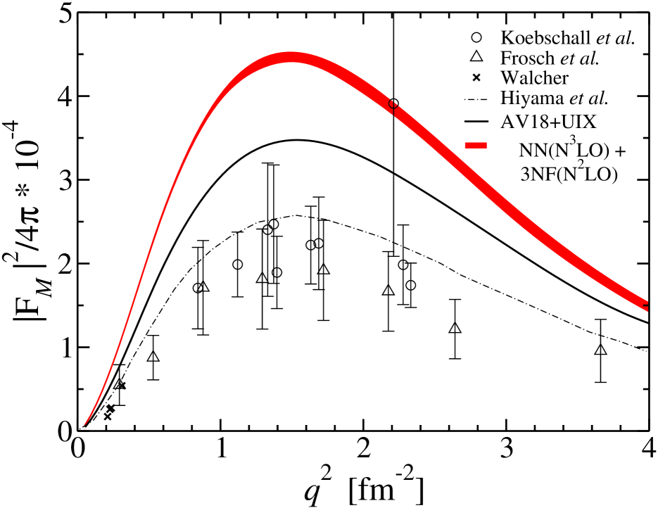
Figure 1: (Color online) Theoretical transition form factor $|F_{\mathcal{M}}(q^{2})|^{2}$ with $G^{n}_{E}=0$ calculated with various force models: AV18+UIX (full line), N³LO+N²LO (red band); result from HiG04 (dot-dashed). Data from Frosch et al. FrR65 , Walcher Wa70 and Köbschall et al. KoO83 .

In Fig. 1, we show results for $F_{\cal M}(q)$ with two different Hamiltonians including realistic three-nucleon forces (3NF) in comparison to experimental data from inelastic electron scattering FrR65 ; Wa70 ; KoO83 . As Hamiltonians we use (i) the AV18 WiS95 NN potential plus the UIX PuP95 3NF, (ii) an EFT based potential, where we take the NN potential EnM03 at fourth order (N³LO) in the chiral expansion augmented by a 3NF at order N²LO Na07 . The Coulomb potential is taken into account in all calculations. Both the EFT and the AV18 NN potentials reproduce the NN scattering phase shifts with high precision ($\chi^{2}/{\rm datum}\approx 1$). In the EFT calculations, two different parameterizations of the 3NF have been used, leading to the red band in Fig. 1. The chiral low energy constants $c_{D}$ and $c_{E}$ have been determined either by setting $c_{D}$ to a reasonable value and then fitting $c_{E}$ to the three-nucleon binding energies Na07 ($c_{D}=1$ and $c_{E}=-0.029$) or by fitting to the ³H binding energy and beta decay GaQ09 ($c_{D}=-0.2$ and $c_{E}=-0.205$). We also display the result of a previous calculation by Hiyama et al. HiG04 , with the AV8’ potential, a reduced version of AV18, and a simplified central 3NF, fitted to the binding energy of ³H. All three Hamiltonians reproduce the ⁴He experimental binding energy within one percent. Surprisingly, the results for $F_{\mathcal{M}}(q)$ strongly depend on the Hamiltonian. Furthermore, the realistic Hamiltonians fail to reproduce the experimental data. In particular, this is true for the EFT forces that predict a transition form factor twice as large as the measured one.

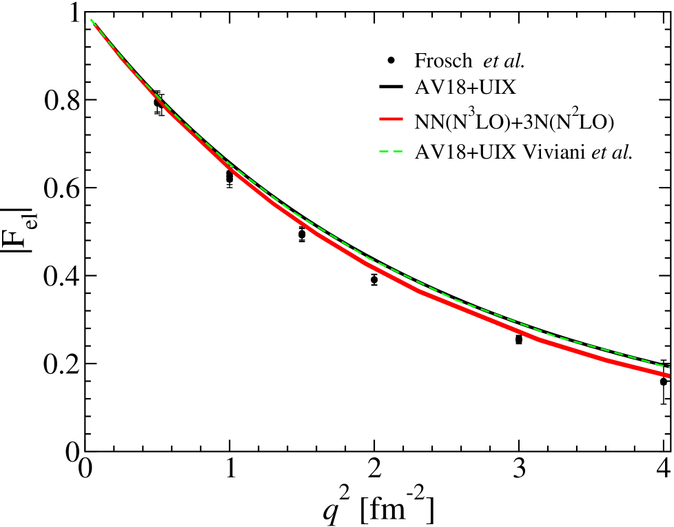
Figure 2: (Color online) Elastic form factor $|F_{el}(q^{2})|$ of ⁴He calculated with various force models: AV18+UIX (full line); N³LO+N²LO (red band); result from ViS07 with AV18+UIX (dot-dashed). Data from Frosch et al. FrM67 .

In contrast, the realistic Hamiltonians lead to rather similar results for the elastic form factor $F_{el}(q)$ of ⁴He, defined as

$$F_{\rm el}(q)=\frac{1}{Z}\left<0\left|\mathcal{M}({q})\right|0\right>\,.$$ (5)

In Fig. 2, $F_{el}(q)$ is shown for the AV18+UIX model and for the chiral EFT potentials. The fact that the results do not differ significantly is not very surprising, since both Hamiltonians give a very similar result for the radius: 1.432(2) fm GaB06 for AV18+UIX and 1.464(2) fm for N³LO plus the N²LO of GaQ09 which is not far from the experimental value of $1.463(6)$ fm (obtained from the charge radius of Ref. Sic08 as explained in correction ). Also shown in Fig. 2 is the result by Viviani et al. ViS07 with the AV18+UIX potential, which is indistinguishable from ours, proving the level of accuracy of contemporary four-body calculations.

Table 1: Ground state energies in MeV for ³H, ³He and ⁴He with N³LO EnM03 and N²LO (parameterizations from Na07 or GaQ09 ). Comparison of present results (EIHH) with no core shell model (NCSM) and hyperspherical harmonics (HH) results.

3NF from Na07	EIHH	NCSM Na07	HH KiR08	Nature
3H	-8.474(1)	-8.473(5)	-8.474	-8.48
3He	-7.734(1)		-7.733	-7.72
4He	-28.357(7)	-28.34(2)	-28.37	-28.30
3NF from GaQ09	EIHH	NCSM GaQ09		Nature
3H	-8.472(3)	-8.473(4)		-8.48
3He	-7.727(4)	-7.727(4)		-7.72
4He	-28.507(7)	-28.50(2)		-28.30

Calculational Method.

Our calculations are based on the diagonalization of the Hamiltonian on a square integrable hyperspherical harmonics (HH) basis. The HH convergence is accelerated using the Suzuki-Lee unitary transformation, which then leads to the Effective Interaction HH (EIHH) method [23,24]. The high accuracy of this approach can be inferred from the benchmark results in Ref. KaN01 and also here from Table I, where we present the binding energies of three- and four-body nuclei obtained from EFT potentials including 3NF. We agree with other methods at the 10 keV level.

Results for $S_{\cal M}(q,\omega)$ are often obtained by discretizing the continuum, where the Hamiltonian is represented on a finite basis of square integrable functions and is then diagonalized to obtain eigenvalues $e_{\nu}$ and eigenfunctions $|\nu\rangle$. In this way one achieves an ill defined discretized representation of $S_{\cal M}(q,\omega)$. On the contrary in the Lorentz integral transform (LIT) approach ELO94 ; EfL07 a continuum discretization can be properly used to reach the correct continuum spectrum (for various benchmark tests of the LIT approach we refer to Ref. EfL07 ).

In the LIT case one has

$${\cal L}_{\cal M}(q,\sigma,\Gamma)=-\frac{1}{\pi}{\it Im}\langle 0|{\cal M}^{\dagger}(q)\frac{1}{\sigma-H+E_{0}+i\Gamma}{\cal M}(q)|0\rangle\,,$$ (6)

where $\Gamma$ is finite (compare with Eq. (1)). It is easy to prove that ${\cal L}_{\cal M}(q,\sigma,\Gamma)$ is connected to $S_{\cal M}(q,\omega)$ by an integral transform with a Lorentzian kernel $K(\omega,\sigma,\Gamma)=\frac{\Gamma}{\pi}\frac{1}{(\omega+E_{0}-\sigma)^{2}+\Gamma^{2}}$,

$${\cal L}_{\cal M}(q,\sigma,\Gamma)=\int d\omega\,K(\omega,\sigma,\Gamma)\,S_{\cal M}(q,\omega)\,.$$ (7)

Since $\Gamma$ is finite the calculation of ${\cal L}_{\cal M}(q,\sigma,\Gamma)$ is a bound-state like problem and thus it is legitimate to represent the Hamiltonian on a basis of square integrable functions, which then leads to the following expression:

$${\cal L}_{\cal M}(q,\sigma,\Gamma)=\frac{\Gamma}{\pi}\sum_{\nu=1}^{N}\frac{|\langle\nu|{\cal M}(q)|0\rangle|^{2}}{(\sigma-e_{\nu}+E_{0})^{2}+\Gamma^{2}}\,.$$ (8)

The number of basis functions $N$ depends in our EIHH calculation on the maximal value $K_{\rm max}$ of the HH grand angular momentum quantum number $K$. Note that the set ($e_{\nu}$, $|\nu\rangle$) is $\Gamma$-independent, but that the convergence of ${\cal L}_{\cal M}$ is strongly correlated with $\Gamma$: if $\Gamma$ is lowered a higher density of states is needed, hence $K_{\rm max}$ and thus $N$ have to be increased. In our present case we reached convergence of ${\cal L}_{\cal M}$ with $\Gamma$ as small as 5 MeV employing more than $10^{5}$ states $|\nu\rangle$. Even if this is not sufficient to resolve the ⁴He* resonance width of 270 keV, we are nevertheless able to determine the resonance energy $E_{R}$. In fact our discrete spectrum shows as first excitation above the ⁴He ground state a very pronounced state with strength $s_{1}(q)=|\langle 1|{\cal M}(q)|0\rangle|^{2}$, thus we identify the corresponding energy $e_{1}$ with $E_{R}$. We find the following results: $E_{R}=-7.40(20)$ MeV (AV18+UIX) and $E_{R}=-7.50(30)$ MeV (N³LO+N²LO). Note that error estimates are made by studying the EIHH convergence, i.e. the $K_{\rm max}$ dependence of $E_{R}$ and that the $E_{R}$ value for N³LO+N²LO is obtained extrapolating to higher $K_{\rm max}$ with an exponential ansatz $E(K_{\rm max})=E^{\infty}+ae^{-bK_{\rm max}}$ as in extrap .

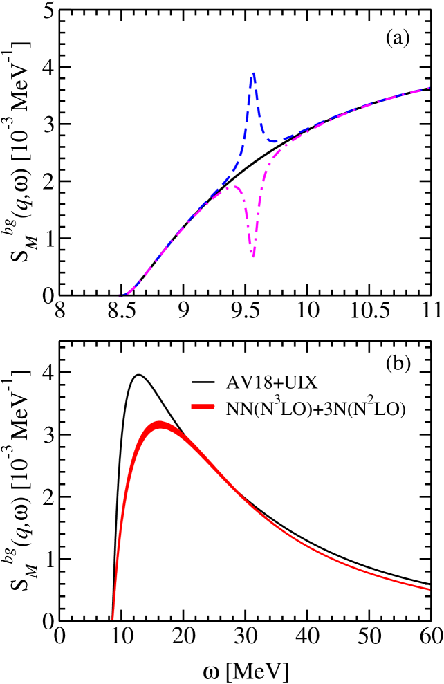
Figure 3: (Color online) (a) ${\cal S}_{\cal M}^{bg}(q,\omega)$ at $q=1.5$ fm^-1 for AV18+UIX obtained with different values of $f_{R}$ (see text): $f_{R}=|F_{\cal M}(q)|^{2}$ (full line), $f_{R}=0.99|F_{\cal M}(q)|^{2}$ (dashed line); $f_{R}=1.01|F_{\cal M}(q)|^{2}$ (dot-dashed line); (b) non-resonant background contribution ${\cal S}_{\cal M}^{bg}(q,\omega)$: AV18+UIX (full line); N²LO+N³LO (red band).

In general one obtains the full strength $S(q,\omega)$ from the inversion of a converged LIT, but one has to be aware that structures much smaller than $\Gamma$ cannot be resolved and thus a regularization procedure has to be used TiA77 ; AnL05 . Our standard inversion method consists in an expansion of the response on a set of $I$ continuous functions and in fitting the calculated ${\cal L}_{\cal M}(q,\sigma,\Gamma)$ on the corresponding linear combinations of the transformed basis functions AnL05 . Note that the regularization consists in the fact that $I$ should not become so large that structures much smaller than $\Gamma$ appear in the inversion result. We implement many different basis and choose the best fit for a given $I$ (for example we use basis sets of the form $E^{\beta}exp(-\alpha E/i)$ with $i=1,...,I$ and different $\alpha$ values; $\beta$ is known from threshold behavior of the response, e.g. $\beta=1/2$ for $S_{\cal M}$). For example, such a calculation has been made in Refs. BaB09a ; BaA07 for the full ⁴He longitudinal response beyond the ⁴He* resonance.

In the presence of a narrow resonance, as in our case, an explicit resonance should be added to the basis, e.g., a Lorentzian with free parameters $\gamma$ and $\omega_{R}$: $[(\omega-\omega_{R})^{2}+(\gamma/2)^{2}]^{-1}$. If the LIT is determined with a sufficiently small $\Gamma$, then position, width, and strength of the resonance can be determined in the inversion Le08 . If we proceed in this way in our present case, imposing $\omega_{R}=E_{R}$, we obtain the best fits with $\gamma\rightarrow 0$. This reflects the absence of states $|\nu\rangle$ in the vicinity of $E_{R}$. We can nonetheless determine, besides $E_{R}$, also the resonance strength $f_{R}(q)$. For this purpose we note that the above defined strength $s_{1}(q)$ is equal to the sum of $f_{R}(q)$ and a background contribution. Thus, formally, we can separate the resonance contribution from ${\cal L}_{\cal M}$:

$${\cal L}^{bg}_{\cal M}(q,\sigma,\Gamma)={\cal L}_{\cal M}(q,\sigma,\Gamma)-\frac{\Gamma}{\pi}\frac{f_{R}(q)}{(\sigma-E_{R}+E_{0})^{2}+\Gamma^{2}}\,.$$ (9)

Now we proceed as follows. We assume a value for $f_{R}(q)$ and allow a basis function of Lorentzian shape centered at $E_{R}$ with $\gamma=100$ keV in the inversion. If the trial value for $f_{R}(q)$ is too small/large one finds an inversion with a positive/negative resonant structure. The case where this vanishes corresponds to the correct value of the transition form factor $|F_{\cal M}(q)|^{2}=f_{R}(q)/Z^{2}$ and the inversion result is just $S_{\cal M}^{\rm bg}(q,\omega)$ (see Fig. 3). We would like to emphasize that the results are almost $\gamma$-independent so long $\gamma$ remains small enough ($0<\gamma\leq 200$ keV) that the Lorentzian approximates sufficiently well a $\delta$-function. For the AV18+UIX potential the relative size of the background reduction, about 8%, is roughly $q$ independent. For the N³LO+N²LO interactions the reduction varies between $13\%$ for $q=0.25\,\rm{fm}^{-1}$ and $22\%$ for $q=2\,\rm{fm}^{-1}$.

In Fig. 3b, the non-resonant monopole strength $S_{\cal M}^{\rm bg}$ is shown on a larger energy range, into the far continuum region. One sees quite a difference between the results with the EFT and the AV18+UIX forces. The former leads to a lower low-energy peak and tail than the latter. These results show the power of the LIT approach, which enables one to calculate the strength in the far four-body continuum by reducing a scattering-state problem to a bound-state problem in a rigorous way.

Analysis of the Results.

The main findings of this Letter are the dramatic sensitivity of $F_{\mathcal{M}}(q)$ to the nuclear Hamiltonian and the large deviations of realistic calculations from the available experimental data. Even though one can contemplate the possibility of systematic experimental errors, the fact that the experimental results of Fig. 1 correspond to three different sets of data, makes it less likely. Thus we will now list possible sources for theoretical uncertainties.

Table 2: $|F_{\rm el}|$ and $s_{1}=|\langle 1|{\cal M}(q)|0\rangle|^{2}$ for $q=1.01$ fm^-1 as a function of the grandangular momentum $K_{\rm max}$ with N³LO+N²LO GaQ09 .

$K_{\rm max}$	12	14	16	18
$|F_{\rm el}|$	0.6248	0.6244	0.6242	0.6241
10${}^{4}s_{1}/4\pi Z^{2}$	4.59	4.75	4.85	4.87

(i) Is our EIHH expansion sufficiently convergent? As shown in Table 2 for a $q$-value of 1.01 fm^-1, we find an excellent convergence for both $F_{\rm el}$ and $s_{1}$.
(ii) Are there relevant two-body corrections to the one-body operator of Eq. (2)? Such corrections are of relativistic order and appear also in EFT only at 4th order Park (also for $F_{\rm el}(q)$ such two-body terms are negligible below $q=2$ fm^-1 ViS07 ).
(iii) Can additional 3NF terms change the picture? This is not excluded, however we notice that the 3NF effect at N²LO on $F_{\cal M}(q)$ is rather mild (about 10%).
(iv) Does the improper theoretical resonance position $E_{R}$ affect the $F_{\cal M}(q)$ result? Both our potential models (AV18+UIX, N³LO+N²LO) overestimate $E_{R}$ by almost the same amount (about $700$ keV), but still lead to quite different transition form factors. On the other hand, the simplified force model used by Hiyama et al. HiG04 reproduces the correct $E_{R}$ within $100$ keV, and also leads to a much better description of $F_{\cal M}(q)$. One can envisage a correlation between the ability of a model to reproduce $E_{R}$ and $F_{\cal M}$. In fact, if one considers that $F_{\cal M}$ is the Fourier transform of the transition density from ⁴He to ⁴He*, one can imagine that small differences in $E_{R}$ are reflected in the resonant wave functions and yield larger differences in the transition density. Similar conclusions have been drawn in Ref. La09 in the study of $p\,$-³H scattering. However, the resonant behavior of the nuclear scattering amplitude is barely visible in the data, in contrast to the electromagnetic probe that amplifies the resonance signal considerably (see Fig. 1 of Ref. KoO83 ).

Conclusions.

We have calculated the isoscalar monopole ⁴He $\longrightarrow^{4}$He* transition form factor $F_{\mathcal{M}}(q)$ with realistic nuclear forces (N³LO+N²LO, AV18+UIX). Unexpectedly the results are strongly dependent on the Hamiltonian. Therefore this observable is ideal for testing nuclear Hamiltonians. As surprising as the large potential model dependence, is the fact that our $F_{\cal M}$ results are at variance with the experimental data, particularly large differences are found in the case of the chiral forces. It is very unlikely that corrections to the isoscalar monopole operator can lead to large effects. In order to clarify the situation it is highly desirable to have a further experimental confirmation of the existing data and in particular with increased precision. On the theory side further insight could be gained by an analysis of sum rules, transition densities, effects of D-wave components and different 3NFs. These issues will be the subject of future studies.

We would like to thank Thomas Walcher for his helpful discussions and explanations about the experiments. We would like to thank Michele Viviani for providing us with his theoretical results for $F_{\rm el}$. Acknowledgments of financial support are given to Natural Sciences and Engineering Research Council (NSERC) and the National Research Council of Canada, S.B., the Israel Science Foundation (Grant number 954/09), N.B., the MIUR grant PRIN-2009TWL3MX, W.L. and G.O.. We would also like to thank the INT for its hospitality during the preparation of this work (INT-PUB-12-050).

References

- (1) D.H. Youngblood et al., Phys. Rev. Lett. 39, 1188 (1977).
- (2) O. Bohigas, A. M. Lane, and J. Martorell, Phys. Rep. 51, 267 (1979).
- (3) J.P. Blaizot, Phys. Rep. 64, 171 (1980).
- (4) Th. Walcher, Phys. Lett. B, 31, 442 (1970).
- (5) S. Fiarman and W.E. Meyerhof, Nucl. Phys. A, 206 1 (1973); D.R. Tilley, H.R. Weller, G.M. Hale, Nucl. Phys. A, 541 1-104 (1992).
- (6) W. Leidemann and G. Orlandini, arXiv:1204.4617; Progr. Part. Nucl. Phys., in press.
- (7) S. Weinberg, Phys. Lett. B 251, 288 (1990); C. Ordóñez, L. Ray, U. van Kolck, Phys. Rev. Lett. 72, 1982 (1994); E. Epelbaum, W. Glöckle, U.-G. Meißner, Nucl. Phys. A 637, 107 (1998).
- (8) A. Kievsky, Few-Body Syst. 50, 69 (2011).
- (9) S. Galster et al., Nucl. Phys. B 32, 221 (1971).
- (10) E. Hiyama, B.F. Gibson, and M. Kamimura, Phys. Rev. C 70, 031001 (R) (2004).
- (11) R.F. Frosch et al., Phys. Lett. 19, 155 (1965); Nucl. Phys. A, 110, 657 (1968).
- (12) G. Köbschall et al., Nucl. Phys. A, 405, 648 (1983).
- (13) R.B. Wiringa, V.G.J. Stoks, and R. Schiavilla, Phys. Rev. C 51, 38 (1995).
- (14) B.S. Pudliner et al., Phys. Rev. Lett. 74, 4396 (1995).
- (15) D.R. Entem and R. Machleidt, Phys. Rev. C 68, 041001 (2003).
- (16) P. Navrátil, Few Body Syst., 41, 117 (2007).
- (17) D. Gazit, S. Quaglioni, and P. Navrátil, Phys. Rev. Lett. 103, 102502 (2009).
- (18) M. Viviani et al., Phys. Rev. Lett. 99, 112002 (2007).
- (19) R.F. Frosch et al., Phys. Rev. 160, 874 (1967).
- (20) D. Gazit et al., Phys. Rev. Lett. 96 112301 (2006).
- (21) I. Sick, Phys. Rev. C 77, 041302R (2008).
- (22) The charge radius is converted to a point-proton radius by where is the proton finite size, =-0.1161(22) is the neutron finite size correction and the last term is a relativistic correction.
- (23) N. Barnea, W. Leidemann, and G. Orlandini, Phys. Rev. C 61, 054001 (2000); Nucl. Phys. A 693, 565 (2001).
- (24) N. Barnea and A. Novoselsky, Phys. Rev. A 57, 48 (1998); Ann. Phys. (N.Y.) 256, 192 (1997).
- (25) H. Kamada et al., Phys. Rev. C 64, 044001 (2001).
- (26) A. Kievsky et al., J. Phys. G 35, 063101 (2008).
- (27) V. D. Efros, W. Leidemann, and G. Orlandini, Phys. Lett. B 338, 130 (1994).
- (28) V. D. Efros et al., J. Phys. G, 34, R459 (2007).
- (29) A.N. Tikonov and V.Y. Arsenin, Solutions of Ill–Posed Problems, Washington, DC: V H Winston and Sons, 1977.
- (30) D. Andreasi et al., Eur. Phys. J. A 24, 361 (2005).
- (31) S. Bacca et al., Phys. Rev. C 80, 064001 (2009).
- (32) S. Bacca et al., Phys. Rev. C 76, 014003 (2007).
- (33) S. Bacca et al., Eur. Phys. J. A 42 553 (2009).
- (34) W. Leidemann, Few-Body Syst. 42, 139 (2008).
- (35) T.-S. Park et al., Phys. Rev. C 67, 055206 (2003).
- (36) R. Lazauskas, Phys. Rev. C 79, 054007 (2009).