Finding New High-Redshift Quasars by Asking the Neighbours

Abstract

Quasars with a high redshift (z) are important to understand the evolution processes of galaxies in the early universe. However only a few of these distant objects are known to this date. The costs of building and operating a 10 -metre class telescope limit the number of facilities and, thus, the available observation time. Therefore an efficient selection of candidates is mandatory. This paper presents a new approach to select quasar candidates with high redshift ($\rm{z}>4.8$) based on photometric catalogues. We have chosen to use the $\rm{z}>4.8$ limit for our approach because the dominant Lyman $\alpha$ emission line of a quasar can only be found in the Sloan $i$ and $z$-band filters. As part of the candidate selection approach, a photometric redshift estimator is presented, too. Three of the 120,000 generated candidates have been spectroscopically analysed in follow-up observations and a new $\rm{z}=5.0$ quasar was found. This result is consistent with the estimated detection ratio of about 50 per cent and we expect 60,000 high-redshift quasars to be part of our candidate sample. The created candidates are available for download at MNRAS or at http://www.astro.rub.de/polsterer/quasar-candidates.csv.

1 Introduction

In the late 1950’s, observations in the radio regime discovered quasi-stellar radio sources with no optical counterpart. Later, a quasar was found to be a distant galaxy with an active galactic nucleus (AGN). An AGN is a central super-massive black hole which accretes material and thereby creates radiation. This phenomenon is seen in different ways and therefore creates a large number of observable AGN classes (Urry & Padovani, 1995). Antonucci (1993) uniformly describes this zoo of AGNs.

Due to their extreme luminosity, even very distant quasars can be observed. This allows to study processes in the early universe. Another benefit of their intrinsically high luminosity is the possibility to find these sources even in surveys with low detection levels. A representative sample of high-z quasars would help to understand the formation process of galaxies (White & Frenk, 1991) and the influence of super-massive black holes on galaxy evolution (Cattaneo et al., 2009). The formation of larger galaxies through hierarchical clustering has direct effects on the creation of quasars. Carlberg (1990) found that the birth-rate of quasars is proportional to the rate of mergers of gas-rich galaxies. The presence of an AGN has direct consequences for the hosting galaxy. As soon as the AGN starts to accrete material and to produce radiation, the gas content of the bulge is heated and, in dependence on the strength of the radiation, blown away. This directly leads to a stop of star formation in the bulge (Cattaneo et al., 2009). Currently there are only a few quasars known with a redshift of $\rm{z}>4.8$. Therefore statistics on their number density is not reliable (Cristiani et al., 2004).

As larger optical telescopes tend to improve both sensitivity and spatial resolution, the field of view is reduced correspondingly. A reduced field of view requires an appropriate selection of targets based on previous observations. Today, large panoramic catalogues are available which can be used for the target selection process.

The presented method of photometrically selecting high-redshift quasar candidates is based on the Sloan Digital Sky Survey (SDSS) DR6 (York et al., 2000; Adelman-McCarthy et al., 2008). A dedicated 2.5 -metre telescope at the Apache Point Observatory in New Mexico was used to create an imaging and spectroscopic catalogue of the northern Galactic Cap ($9,583\,\rm{deg}^{2}$). Images have been taken in drift-scan mode using five broadband filters ($u$, $g$, $r$, $i$, $z$: 300 nm to 1,000 nm). For a selected sub-sample a spectroscopic analysis has been conducted with a fibre-fed spectrograph. In total 287 million objects are stored in the catalogue of which 1.27 million have associated spectra.

The increasing amount of data which is available in catalogues can no longer be handled manually. It requires an automated processing and selection of scientifically important objects. The spectroscopically observed objects have been automatically classified by correlating them with 33 template spectra. In Schneider et al. (2010) a hand-vetted catalogue of 105,783 spectroscopically confirmed quasars is presented. This catalogue contains 1,248 objects with $\rm{z}>4.0$ whereof 56 objects have a redshift of $\rm{z}>5.0$. It is used as a reference set for the presented photometric selection method.

Throughout this paper we adopt a flat $\Lambda$CDM cosmology with $H_{0}=70.2\,{\rm km\,s^{-1}\,Mpc^{-1}}$ and $\Omega_{\Lambda}=0.727$ (Komatsu et al., 2011).

Outline:

The presented technique to select quasar candidates is realised by combining a redshift estimation and a classification approach. In Section 2 the redshift estimator and the used reference sample are presented. The classification approach and the way we compose the multi-stage classifier are described in Section 3. In Section 4 the generated candidate sample is presented (along with theoretical number expectations), and the results of follow-up observations are discussed. Section 5 concludes this work.

2 Photometric Redshift Estimation

An efficient creation of a high-z quasar candidate catalogue requires a precise photometric estimation of the redshift. These estimates allow the rejection of candidates with a redshift below a certain threshold. Photometric methods try to detect the position of strong emission and absorption features which are unresolved in the broadband filters. In Figure 1 the spectra of two high-z quasars are presented together with the filter bands of SDSS. The Lyman $\alpha$ emission lines of these quasars dominate the flux in the $r$ and $i$-band, respectively.

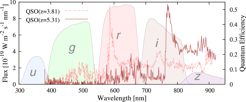
Figure 1: Spectra of the high-z quasar SDSS J082547.79+332836.9 ($\rm{z}=3.81$) and SDSS J165902.12+270935.1 ($\rm{z}=5.31$). In the background the wavelength dependent quantum-efficiency of the $u$, $g$, $r$, $i$, $z$-bands of the SDSS are plotted. The Lyman $\alpha$ emission line of the quasar is red-shifted to the $r$ and $i$-band.

2.1 Related Work

Several methods for photometric redshift estimation can be found in the literature. These estimation methods either rely on physical assumptions or on the quality of the considered reference set. We will briefly discuss these two concepts.

2.1.1 Template Fitting

A classical way of photometric redshift estimation is the fitting of spectral energy distributions (SEDs). This method is typically limited to a small set of representative model spectra. These spectra can be created based on empirical or simulated SEDs. In Bolzonella et al. (2000), an estimation method using a $\chi^{2}$-minimisation is presented. The quality of the fit is highly dependent on the applied template spectra. When the used photometric features do not allow to distinguish between the different SEDs, the fit can create catastrophic outliers. The big advantage of the SED fitting approach is the ability to predict rough estimates even for objects with spectroscopically yet unobserved redshifts.

Wu & Jia (2010) present a photometric redshift estimator that combines SDSS and UKIRT Infrared Deep Skey Survey (UKIDSS) data. A reference sample of 7,400 quasars with $0.5<\rm{z}<5.2$ was divided into 91 redshift bins. Each bin was analysed and a median colour was calculated for the eight directly neighbouring bands. The most probable redshift is retrieved by applying a $\chi^{2}$-minimisation of colours with respect to the photometric errors. As a result of their tests, 71.8 per cent of their reference sample have a redshift estimation error of $|\rm{z_{spec}-z_{est}}|<0.1$.

2.1.2 Neural Networks

Another way of redshift estimation is based on empirical reference data. In O’Mill et al. (2011), such an approach is presented for the SDSS data. Here, 80 per cent of the main galaxy sample (Strauss et al., 2002), 10 per cent of the luminous red galaxy sample (Eisenstein et al., 2001), and 10 per cent of the active galactic nuclei sample (Kauffmann et al., 2003) have been combined to a set of 550,000 objects with spectroscopic redshifts. Half of this reference set was used for training an artificial neural network and the other half for testing. The input nodes represent the SDSS magnitudes, the concentration index and the Petrosian radii in the $g$ and $r$-band. Three hidden layers, of 14 neurons each, have been used to calculate the redshift output. They limited their tests to a redshift range of $\rm{z}<0.4$. In this range their estimates deviate from the spectroscopically determined redshifts with an $\rm{rms}\approx 0.03$.

Laurino et al. (2011) consider combining a clustering approach with neural networks. To build the model, the data is clustered in the feature space. These clusters are used to train individual neural networks and, thus, to obtain a more flexible regression model.

2.2 k-Nearest Neighbours

In Section 3, we present a new quasar selection method. Fundamental for this selection is a reliable photometric redshift estimation. A new redshift estimator was developed which is based on empirical data. It was designed to process large reference sets without requiring physical assumptions or models. This estimator realises the important step of rejecting candidates with low redshifts. It uses a k-nearest neighbours (kNN) regression model to predict redshifts (Hastie et al., 2009).

2.2.1 Regression Model

Given the reference sample $S=\{({\bf x}_{1},y_{1}),\ldots,({\bf x}_{n},y_{n})\}\subset{\mathbb{R}}^{d}\times{\mathbb{R}}$, the predicted redshifts $\hat{Y}$ are calculated from the redshift values $y_{i}$ of the $k$ Euclidean closest objects. Thereby the neighbourhood $N_{k}({\bf x})$ is determined on basis of the representation of the reference objects ${\bf x}_{i}$ in the feature space:

$$\hat{Y}({\bf x})=\frac{1}{k}\sum\limits_{{\bf x}_{i}\epsilon N_{k}({\bf x})}y_{i}$$ (1)

To retrieve these $k$ neighbours $N_{k}({\bf x})$ of ${\bf x}$ efficiently, a $k$-d-tree is used (Bentley, 1975). This data structure is a binary search tree that allows a spacial look-up in ${\mathcal{O}}(\log_{2}n)$ instead of ${\mathcal{O}}(n)$ time. Besides the redshift value the standard deviation of the $k$ nearest $y_{i}$ is calculated as a quality measure. High standard deviations indicate a bad coverage of the target space. To analyse the distribution of reference objects in the feature space, the length of the average distance vector to the $k$ nearest neighbours can be calculated. Large values indicate that the requested object lies in a sparsely populated region of the feature space and might therefore have a very high or low redshift, respectively.

SDSS PhotoObjID	z	Reference
588023045868553340	5.79	Fan et al. (2006)
587740525079167786	5.80	Fan et al. (2004)
587727942951109703	5.82	Fan et al. (2001)
587733411521299389	5.83	Fan et al. (2006)
587731186204541926	5.85	Fan et al. (2004)
587737808499572747	5.85	Fan et al. (2006)
587736914601902923	5.93	Fan et al. (2004)
587738951494075293	5.93	Fan et al. (2006)
587729157893456734	5.99	Fan et al. (2001)
587741421098303812	6.00	Fan et al. (2006)
587738615416554219	6.01	Fan et al. (2006)
587729751132603659	6.05	Fan et al. (2003)
587735666926158831	6.07	Fan et al. (2004)
587739608093491422	6.13	Fan et al. (2006)
587736783608677304	6.22	Fan et al. (2004)
587732482206139341	6.23	Fan et al. (2003)
587728881415553909	6.28	Fan et al. (2001)
588013383815791587	6.43	Fan et al. (2003)

Table 1: High-z quasars which have been found based on the $i$-band dropout method and that have been used to extend the reference sample.

2.2.2 Reference Sample

A reference sample was created to support the detection process of high-redshift quasars, which is based on the SDSS quasar catalogue (Schneider et al., 2010). This sample is used to populate the feature space. To increase the processing speed of estimating redshifts, the size of the reference sample was reduced. For this reason the input catalogue was split into three subsets:

1. The low-redshift ($\rm{z}<2.0$) set with 81,238,

2. the medium-redshift ($2.0\leq\rm{z}<4.0$) set with 22,696,

3. and the high-redshift ($\rm{z}\geq 4.0$) set with 1,258 objects.

As the high-redshift set contains only a few quasars with $\rm{z}\geq 5.0$ and is limited to $\rm{z_{max}}=5.5$, 18 additional objects with SDSS features have been added (see Table 1). To create a homogeneously distributed sample (what we call the reduced sample), all quasars have been assigned to 120 equal bins in redshift space for redshifts between $\rm{z}=1.0$ and $\rm{z}=7.0$. We deliberately excluded all quasars below ${\rm z}=1.0$ since the reference sample is specifically designed for finding high-z quasars. Hence, the many quasars below ${\rm z}=1.0$ would just slow down processing without substantially adding information with respect to the anticipated redshift range. For those bins below $\rm{z}=4.8$, the size was limited to ten reference objects and supernumerous objects have been randomly extracted. Above a redshift value of $\rm{z}=4.8$, all quasars have been included. Due to missing high-z references the high-z bins are not filled equally. The resulting reference sample contains 1,106 quasars with spectroscopically determined redshifts and SDSS magnitudes.

2.2.3 Model Selection

During tests with the kNN regression model it turned out that the best results are achieved when using colours ($u-g$, $g-r$, $r-i$, $i-z$) instead of magnitudes. This may be caused by distribution effects of the reference objects in the Euclidean feature space which are induced by intrinsic object characteristics like their luminosity. These effects are minimised by a kind of normalisation which is obtained by the dimension reduction from filter band to colour space. Colours eliminate the effects of different luminosities because they just reflect differences in flux density and not the flux density itself. Therefore we gain predictive quality by treating faint and bright sources with same redshifts as equal. The $k$-value was set to eight, based on tests of the redshift estimation performance. With smaller $k$-values the standard deviation of the estimation errors increases. Slightly larger values (up to 20) did not significantly improve the results but enhanced the computational effort.

2.3 Evaluation of the Redshift Estimation

The quality of the kNN regression redshift estimation approach was tested on the quasars with spectroscopic redshifts taken from Schneider et al. (2010). As the reference sample is limited to redshifts with $\rm{z}\geq 1.0$, quasars with lower redshifts have been excluded from the tests. There are only a few high redshift quasars known. Therefore all objects are required as reference as well as for testing.

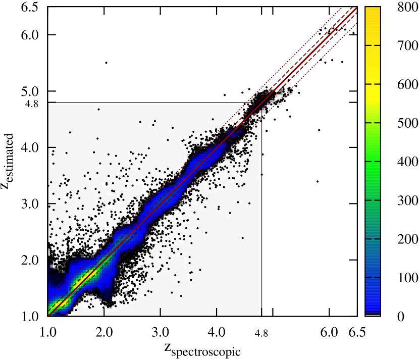
Figure 2: Comparison of estimated and spectroscopic redshifts where the estimation is based on a reference sample consisting of all known quasars above $\rm{z}=1.0$. The mean value, the $1\sigma$- and the $3\sigma$-values of the fitted Gaussian distribution are plotted as a solid, a dashed and a dotted line, respectively. In addition the interesting area of redshifts with $\rm{z}>4.8$ is marked.

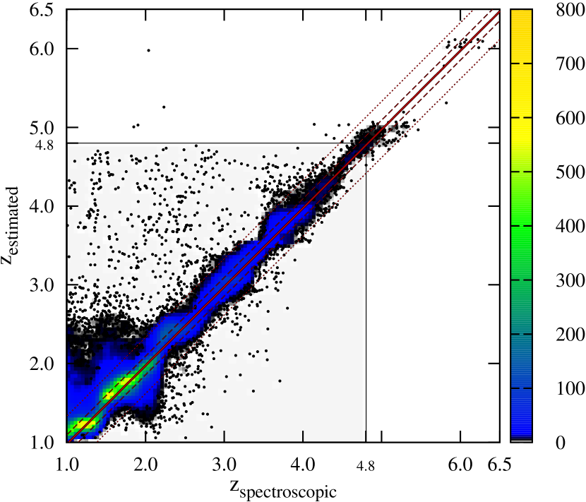
Figure 3: Results of the estimation done with the reduced reference set. The considered $\rm{z}=4.8$ limit, as well as the parameter of the fitted Gaussian distribution are marked, as for Figure 2.

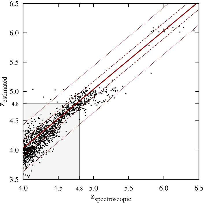
Figure 4: Magnified high-z ($\rm{z}>4.0$) sector of the results of the estimation done with the reduced reference set. Important parameters are marked in the same manner as in the previous figures.

2.3.1 Results

A leave-one-out cross-validation scheme was applied to optain the test results. For each object of the test sample, a deviation $\Delta\rm{z}=\rm{z_{spectroscopy}}-\rm{z_{estimation}}$ and a redshift independent deviation $\Delta\rm{z}/(1+\rm{z_{spectroscopy}})$ was determined. In Figure 2, the results of the estimation approach are presented. The area below $\rm{z}=4.8$ is marked grey because quasar candidates which lie outside of the target redshift range are rejected. The comparison of the results of the reduced reference sample (Figure 3) with the results of the complete reference sample (Figure 2) demonstrates that both sets perform equally well for $\rm{z}>4.8$. In Figure 4, the results of the important $\rm{z}>4.0$ area are shown in a magnified plot. With the reduced reference sample lower red-shifted quasars can still be processed with an appropriate estimation quality, even though the size of the reference set was dramatically reduced from 77,096 to 1,106 objects. As the reduced reference sample is homogeneously distributed in redshift, no catastrophic outliers are produced by an over-representation of lower redshifts. In both Figures (2 and 3), a redshift dependent fluctuation between estimated and spectroscopic values can be observed. This is directly connected to the passage of the Lyman $\alpha$ features through the broadband filters.

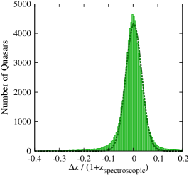
(a) Estimation error of all known $\rm{z}\geq 1.0$ quasars with complete reference sample.

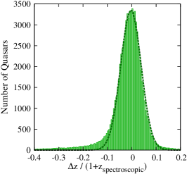
(b) Estimation error of all known $\rm{z}\geq 1.0$ quasars with reduced reference sample.

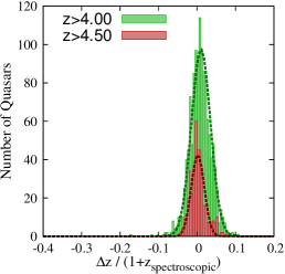
(c) Estimation error of all known $\rm{z}\geq 4.0$ quasars with reduced reference sample.

Figure 5: Histograms of the redshift estimation errors are compared for different reference and test samples. The fitted Gaussian distributions are plotted as double dashed lines.

Reference	Reference Size	Redshift	Test Set Size	$\langle\frac{\Delta\rm{z}}{1+\rm{z}}\rangle$	$\sigma_{\frac{\Delta\rm{z}}{1+\rm{z}}}$	$\langle{\Delta\rm{z}}\rangle$	$\sigma_{\Delta\rm{z}}$
complete	77,096 quasars	$1.0\leq\rm{z}<6.5$	77,096 quasars	0.003	0.033	-0.007	0.091
complete	77,096 quasars	$4.0\leq\rm{z}<6.5$	1,258 quasars	0.008	0.024	-0.065	0.126
complete	77,096 quasars	$4.5\leq\rm{z}<6.5$	406 quasars	0.002	0.021	-0.011	0.117
reduced	1,106 quasars	$1.0\leq\rm{z}<6.5$	77,096 quasars	-0.023	0.095	-0.024	0.119
reduced	1,106 quasars	$4.0\leq\rm{z}<6.5$	1,258 quasars	0.010	0.025	0.036	0.133
reduced	1,106 quasars	$4.5\leq\rm{z}<6.5$	406 quasars	0.002	0.016	0.001	0.087

Table 2: Results of fitting Gaussian distributions to the redshift estimation errors. The values are given for both $\Delta\rm{z}/(1+\rm{z})$ and $\Delta\rm{z}$. Additionally, the errors have been determined on both the reduced and the complete reference sample.

The deviation $\Delta\rm{z}$ and the redshift-independent deviation $\Delta\rm{z/(1+z)}$ was determined for different redshift ranges. The results are presented in Table 2. The distribution of the estimation errors for the full redshift range $1.0<\rm{z}<6.5$ is presented in Figures 5 a and 5 b for the full and the reduced reference sample, respectively. In comparison to the tests on the full redshift range, better results are achieved for the high-redshift quasar (see Figure 5 c). As it was intended, the reduced reference sample performs better on quasars in the targeted selection range with $\rm{z}>4.8$. This is caused by the better representation per redshift bin of $\rm{z}>4.8$ quasars in the feature space.

2.3.2 Comparison

The performance of the redshift estimation is comparable to the results of Wu & Jia (2010), but: (i) Their results are based on a test sample of only 8,498 quasars which was partially (87 per cent) used to create the median colours. This creates a bias on the test results. (ii) SDSS and UKIDSS data were used. (iii) The presented results are dependent on the redshift range and can therefore not be compared directly.

Mortlock et al. (2011) present a Bayesian redshift estimator which is used to assign observation priorities to their high-redshift quasar candidates. Based on photometric data of SDSS and UKIDSS an accuracy of $|\rm{z_{spec}-z_{est}}|\simeq 0.1$ is presented for a redshift range of $5.8<\rm{z}<7.2$. This deviation is comparable to the results achieved with the presented kNN regression model. As there are no quasars known with $\rm{z}>6.5$ in both SDSS and UKIDSS, the results have been computed with simulated SEDs and are based on a modelled high-z quasar population.

In Cardamone et al. (2010), a 32-band data set is used to calculate photometric redshifts. They present a $1\sigma$ scatter in $\Delta\rm{z}/(1+\rm{z})$ of 0.008 for $0.1<\rm{z}<1.2$, 0.027 for $1.2<\rm{z}<3.7$ and 0.016 for $\rm{z}>3.7$, respectively. For the high-redshift range, these results are as good as the results of the kNN regression model which uses only five bands.

A direct comparison with Laurino et al. (2011) indicates a competitive but slightly better performance of our regression model. Creating global models for sub-clusters in the feature space is an improvement compared to using pure global models. The kNN regression model, however, creates local predictions that seem to reflect the sample intrinsic error rate.

The developed redshift estimator exhibits a competitive performance compared to the other presented approaches. Its main benefit is the capability to predict photometric redshifts with comparable quality even with less photometric bands. Additionally the processing speed on large reference samples is increased by using special data structures. The most important advantage of our approach is that no physical assumptions are required at all.

3 Photometric Selection of Quasars

The described estimation of redshifts is dependent on a reliable pre-selection of quasars. The main problem in selecting these candidates is that broadband observations of the high-redshift SEDs of quasars become similar to the SEDs of cool stars. Before describing the kNN-based quasar selection approach and the creation of the required reference samples, an overview of currently available methods is given.

3.1 Related Work

Several methods are applied to find high-redshift quasar candidates. Among these methods are linear and Bayesian models, which we describe next.

3.1.1 Linear Models

In the SDSS, the selection of quasar candidates for spectroscopic observations is based on photometric data (Richards et al., 2002). The magnitudes which are extracted on basis of fits to a point spread function (PSF) are inspected for unresolved objects in distinct 3D colour spaces to separate quasars from stars. Several decision trees have been created that reflect relations in band-flux and thereby define regions in the feature space.

The $\rm{z}>5.8$ quasars that are presented in Fan et al. (2001, 2003, 2004, 2006) have been detected by using an $i$-band dropout technique in combination with 2MASS magnitudes. This technique assumes no detection in the $u$, $g$, $r$-band, a weak detection in the $i$-band, and a detection in the $z$-band. The principle behind this approach is that the strong Lyman $\alpha$ forest absorption enters the $i$-band at $\rm{z}>5.5$. The resulting constraints are: $mag_{z}<20.2$ with $\Delta mag_{z}<0.1$, $mag_{i}-mag_{z}>2.2$ and $mag_{z}-mag_{J}<1.5$. This method turned out to have a high false positive rate. Only about $3$ per cent of the candidates that had follow-up observations were confirmed as quasars.

Wu & Jia (2010) present a quasar selection approach that uses colour-colour relations in SDSS and UKIDSS bands. The best solution to separate quasars from stars was empirically found in the $Y-K$ and $g-z$-colour space with the linear relation $Y-K>0.46(g-z)+0.53$. This relation correctly separates 97.7 per cent of both the 8,498 quasars and 8,996 stars which have been used as reference. Unfortunately this simple linear separation fails for quasars with $\rm{z}>4.0$. For this reason the relation $J-K>0.45(i-Y)+0.64$ has been created to the find 99 per cent of the 101 reference quasars with $\rm{z}>4.0$. The downside of this framework is that the contamination with stars is more than doubled. Another problem of optimising the separating relation is that the equal cardinalities of the reference samples do not necessarily reflect the real distribution. Even at larger distance from the galactic plane the number density of cool stars exceeds the number density of high-redshift quasars by a factor of up to 1,000 (Fan, 1999).

3.1.2 Bayesian Models

Mortlock et al. (2011) present a probabilistic candidate selection approach which uses SDSS and UKIDSS to find the most probable high-z quasars. Their approach is comparable to their redshift estimator. It uses a Bayesian model to separate quasars from stars. Their targeted redshift range is $\rm{z}>5.8$. With their approach a reduction of the primary data set by a factor of about $2.5\times 10^{4}$ to 893 candidates was realised. Thereby the probabilistic evaluation of each object took 0.01 s to 0.1 s. Only 88 of these 893 candidates turned out to be real detections of astronomical sources with three previously known high-z quasars. Follow-up observations left seven photometric candidates of which four have an estimated redshift $\rm{z}\simeq 6.0$. The results of these candidates are not published yet.

3.2 Quasar Selection with a kNN Classifier

The main purpose of the quasar selection scheme presented below is to create quasar candidates with a high probability for follow-up observations. For this reason the number of recovered quasars is set to a lower percentage than in the other presented approaches.

3.2.1 Pre-Processing

As a pre-filtering of all 287 million SDSS objects a limiting $i$-band magnitude of 16.5 mag is used. Brighter objects or objects with an $i$-band error $>0.2$ mag are ignored, since at our redshift cut of $\rm{z}>4.8$, an $i$-band magnitude of 16.5 mag corresponds to a restframe (at 1,450 $\rm\AA$) absolute magnitude of $M_{1450}=-32$. Additionally, only point-like or slightly extended objects are selected. To separate point sources from extended ones SDSS uses the PSF and model magnitudes: When an object complies with $\rm{PSF_{mag}-model_{mag}}>0.145$ in at least two of the three $g$, $r$, $i$-bands, it is labelled as galaxy in the SDSS catalogue. Here, a value of 0.3 is used instead to include slightly extended sources of e.g., possible lensed quasars. The corresponding database query created a sample of 122 million objects with $u$, $g$, $r$, $i$, and $z$-band PSF magnitudes and errors.

3.2.2 Classification Model

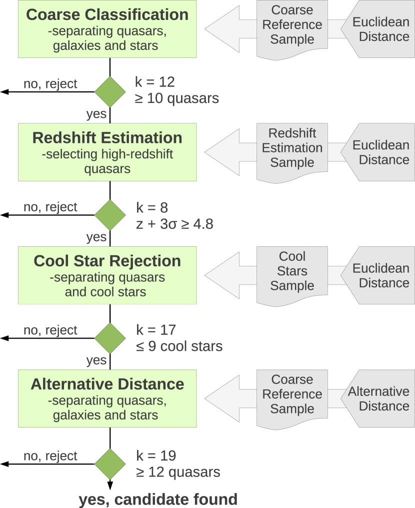
Figure 6: Diagram of the different classifier stages. Both, the required reference sample and the distance function which is used for the neighbourhood search, are presented for every stage. In addition, the selection criteria that have been applied are shown.

Similar to the redshift estimation approach presented in Section 2, the classification is done with the kNN algorithm (Hastie et al., 2009). Based on the reference sample $S=\{({\bf x}_{1},t_{1}),\ldots,({\bf x}_{n},t_{n})\}\subset{\mathbb{R}}^{d}\times T$, the classification of the types $t_{i}$ of the $k$ nearest objects $N_{k}({\bf x})$ in the feature space is evaluated for each ${\bf x}$. The corresponding ratio $\hat{R}_{t}({\bf x})$ reflects the number of the $k$ neighbouring reference objects of ${\bf x}$ that are of a certain type $t\in T$ and is defined as:

$$\hat{R}_{t}({\bf x})=\frac{1}{k}\sum\limits_{{\bf x}_{i}\epsilon N_{k}({\bf x})}q_{i}{\rm{\,with\,}}q_{i}=\begin{cases}1,&t_{i}=t\\ 0,&\rm{otherwise}\end{cases}$$ (2)

The quasar candidate selection is realised by combining the redshift estimator and three classifiers (see Figure 6):

1. The first classifier should realise a coarse quasar pre-selection. This is achieved by using a more general reference set with several object types. The Euclidean distance in the PSF magnitude feature space is used to identify the k nearest neighbours.

2. In the next step, the redshift is estimated and low-redshift objects are rejected (see Section 2).

3. In the third step, a classifier which rejects cool stars is used to decrease the contamination by stellar objects. This is realised by a comprehensive reference sample which contains only cool stars and quasars. The same feature space as for the coarse pre-selection is used.

4. In the last step, an alternative distance measure $d$ is used to run a classification with respect to the photometric errors. The first part of this function reflects the similarity of two feature vectors ${\bf u},{\bf v}\in{\mathbb{R}}^{d}$ with respect to the measurement errors ${\bf{\Delta u}},{\bf{\Delta v}}$:

   $$d({\bf u},{\bf{\Delta u}},{\bf v},{\bf{\Delta v}})=\sum_{i=1}^{N}\frac{(u_{i}-v_{i})^{2}}{\Delta u_{i}^{2}+\Delta v_{i}^{2}}+(|\Delta u_{i}|-|\Delta v_{i}|)^{2}$$ (3)

   The second part ensures that objects with similar errors become closer. When two objects with severely deviating measurement errors are compared, the first distance component decreases due to the dominant error term. This is compensated by the second component.

Name of Sample	Purpose	Sample Composition
		- all 1,258 ${\rm z}\geq 4.8$ high-redshift quasars
		- 1,000 randomly selected $2.0\leq{\rm z}<4.8$ medium-redshift quasars
coarse	coarse preselection,	- 1,000 randomly selected galaxies
	used in stage 1 + 4	- 1,000 randomly selected stars
		- 1,500 randomly selected cool stars
	rejection of cool stars,	- all 1,258 ${\rm z}\geq 4.8$ high-redshift quasars
cool stars	used in stage 3	- all spectroscopically determined cool stars
		- 120 equal redshift bins between $1.0\leq{\rm z}<7.0$
redshift	estimation of redshift,	with a maximum of 10 quasars per bin
	used in stage 2	- all ${\rm z}\geq 4.8$ high-redshift quasars

Table 3: The reference samples that are used for selecting quasar candidates and for estimating the redshifts.

3.2.3 Reference Samples

The classifiers require reference samples similar to the presented redshift estimator sample. All object classifications which are used to create the samples are based on spectroscopic observations (see Table 3). The first sample was created to detect quasars and represents five different types. The second table contains 10,928 objects and is used to reject cool stars. By using spectroscopically classified objects and objects detected by the $i$-band dropout method as reference, the applied sample selection criteria (Richards et al., 2002; Fan et al., 2001, 2003, 2004, 2006) are reproduced by the presented reference samples. Furthermore the objects selected as quasar candidates by Richards et al. (2002) that turned out to be cool stars improve the separation capabilities of the samples.

3.2.4 Model Selection

In each step of the selection process, objects that do not match the ratio criteria are rejected. The ratios have been created on basis of the SDSS objects with spectroscopic classifications. They have been optimised to find as many high-z quasars as possible while simultaneously minimising the contamination by other objects.

1. For the coarse pre-selection step, a ratio of $10/12$ high-z quasars was determined.

2. The redshift estimator is used to exclude objects with $\rm{z}\leq 4.8$. The standard deviation that is calculated based on the k nearest neighbours is used to allow an undershooting of this $\rm{z}$ value by $3\sigma$.

3. For the cool stars rejecting classifier a ratio of $8/17$ quasars was empirically found to produce the best results. This means that ten or more cool stars are required to reject a candidate.

4. In the last selection step, the 19 nearest neighbours are inspected. Twelve of these neighbours must be high-z quasars to pass this step.

3.2.5 Post-Processing

The objects that pass all four selection steps are written to a result file. Instead of simple ratios it contains the types of the 20 nearest neighbours for each step. This allows a post-processing to reduce the candidate list for follow-up observations. The likelihood of a candidate being a high-z quasars can be estimated by calculating different ratios afterwards. Thereby constraints can be combined. These constraints can be separately specified for each of the classifiers.

3.3 The Evaluation of the Selection Approach

To evaluate the performance of the presented selection approach, all 1.2 million SDSS objects with spectra have been photometrically analysed.

3.3.1 Results

Applying our approach for identifying ${\rm z}>4.8$ quasars to the 1.2 million SDSS objects with spectra, we obtained a list of 242 candidate high-z quasars. We note that we explicitly excluded all such objects from neighbourhood queries that were also used in one of the reference data sets for training the model in order to prevent any biasing of our results. The spectra of all of these 242 quasar candidates have been visually inspected subsequently and their types have been checked. 147 of these candidates are quasars of the high-z reference sample with $\rm{z}>4.0$. 75 of the known 147 quasars with $\rm{z}>4.8$ are recovered by the photometric selection. The 18 quasars of the high-z extension sample have been tested separately as they are not part of the SDSS spectroscopic catalogue. 17 of these quasars can be detected with the photometric selection approach. For these objects that have been found with an $i$-band dropout method the coarse classifier calculates ratios of $\geq 19$ out of 20. Of all 32,210 known cool stars, only 34 have been falsely classified as quasars. The spectra of the remaining 61 objects are of other types or are not assignable to a type.

4 Results

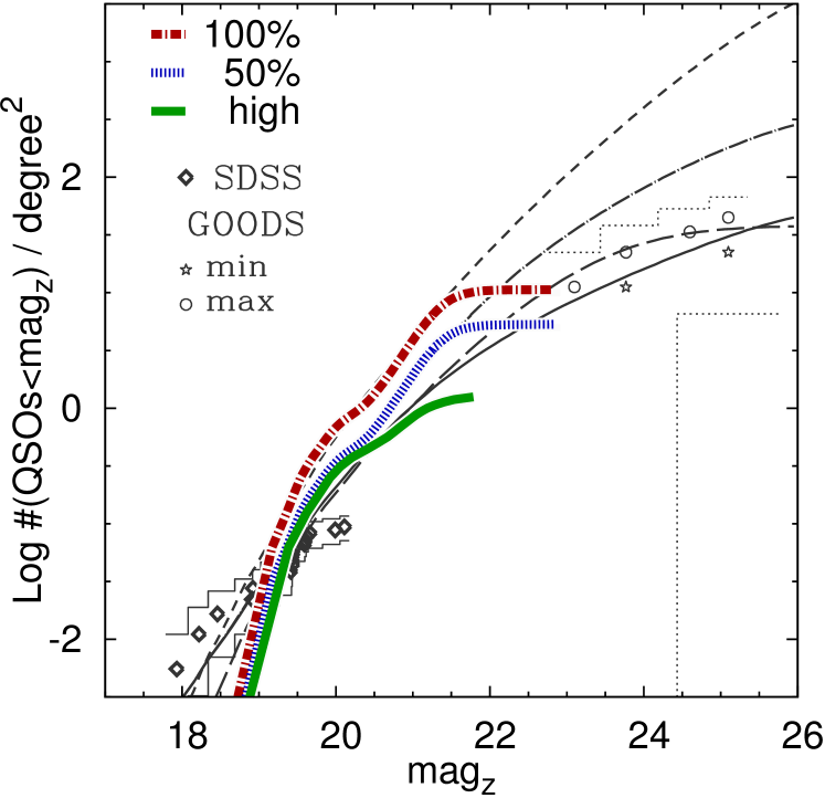
Figure 7: Comparison of the space density plot of quasars ($4.0<\rm{z}<5.2$) from Cristiani et al. (2004) and the parameters derived from the created candidate sample. Circles and stars show the GOODS based estimates of Cristiani et al. (2004) while diamonds are used for SDSS results. The tiny dashed lines represent the upper and lower $1\sigma$ confidence level of the GOODS data. The models that have been used by Cristiani et al. (2004) are: PLE (dot-dashed), PDE (continuous), MIN (short-dashed) and DEL (long-dashed). The three coloured lines represent the entire candidate sample (100 per cent), an assumed detection performance (50 per cent) and the candidates with the highest ratios $\hat{R}$.

Finally, we used our approach to search the entire $DR6$ photometric database for high-z QSOs. The $DR6$ database contains about 122 million objects down to $i$-band magnitudes of $\sim 21.5$ which is more than two magnitudes deeper than the limiting magnitude for SDSS spectroscopy. We therefore anticipate to reveal a great number of formerly unconsidered QSOs with ${\rm z}>4.8$ to be potential targets for future spectroscopic follow-up. The pre-selected 122 million objects have been processed with our approach and a list was created. We obtained a list of 121,909 objects that match the specified ratio criteria of the individual selection steps and are hence regarded as high-z quasar candidates. The sample contains redshift estimations for 82,358 candidates with $\rm{z}<5.0$, 34,359 with $5.0\leq\rm{z}<6.0$ and 5,193 with $\rm{z}\geq 6.0$. The detection performance was calculated on the spectroscopic sample to be about $50$ per cent. A machine-readable version of the sample in comma separated value format can be downloaded at MNRAS or directly at http://www.astro.rub.de/polsterer/quasar-candidates.csv. It contains the original SDSS photometric ID, position, estimated redshift and its standard deviation, the three ratios from the different stages of the classifiers and the PSF magnitudes in all five SDSS bands. The redshift estimations have to be treated carefully and should just be used as an indication. Especially the high-z area is so underrepresented in the sample that a high standard deviation of the redshift estimation indicates a possible outlier.

Under the assumption that the classifier performs comparably on the photometric sample, $\approx 60,000$ high-z quasars are part of the candidate list.

4.1 Comparison with Theoretical Models

Cristiani et al. (2004) presented a space density for quasars with $4.0<\rm{z}<5.2$. A separate classification run for this redshift range yielded a list of 102,825 candidates. In Figure 7 these candidates are plotted in comparison with the results of Cristiani et al. (2004). The red line is a cumulative plot of all candidates while the blue line assumes a quasar detection performance of about $50$ per cent. When the ratio of the first selection step is set to the highest possible ratio (i.e. twelve quasars under the twelve nearest neighbours) only 12,586 candidates remain. These candidates with the highest probability of being a quasar are plotted as a green line.

The presented results are consistent with the results of Cristiani et al. (2004) and the number of found quasar candidates fits well with the presented models. A model which connects quasars and dark matter halos with a minimal set of assumptions (MIN) is presented by Haiman & Hui (2001). This model assumes: (i) an un-evolved halo, (ii) a constant black hole to dark matter halo mass ratio (iii) and a maximum accretion at the Eddington limit (Cristiani et al., 2004). As this model overpredicts high-z quasars (Haiman et al., 1999), it defines an upper limit for the presented candidate selection approach. Monaco et al. (2000) present a model with a delayed quasar shining (DEL) in which the AGN activity starts after the formation of the dark matter halo. In their model, AGNs which are hosted in smaller halos are longer delayed than those AGNs in larger halos. This allows brighter quasars to appear before the fainter ones. The pure luminosity evolution (PLE) model (brighter objects in the past) and the pure density evolution (PDE) model (higher object density in the past) are used in Cristiani et al. (2004) to extrapolate the results of Boyle et al. (2000). Both, the high ratio results as well as the results of the predicted detection performance fit well with these models. In DR6 of the SDSS the 95 per cent detection repeatability for point sources in the $z$-band is 20.5 mag. For this reason the results with the highest probability deviate from the model fits for higher $z$-band magnitudes. The results of the other candidate lists fit well for $z$-band magnitudes below 21.5 mag. In comparison to the quasars detected in the SDSS, an appropriate amount of candidates can be found even for $z$-band magnitudes fainter than 19.5 mag (see Figure 7).

4.2 Spectroscopic Verification of Candidates

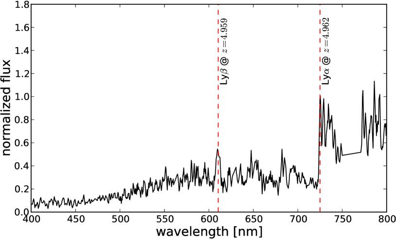
Figure 8: Reduced spectrum of J1538+5032 (SDSS ID 588011218070144145), a newly found quasar with a redshift of $\rm{z}\sim 5.0$. Taken with SCORPIO@BTA.

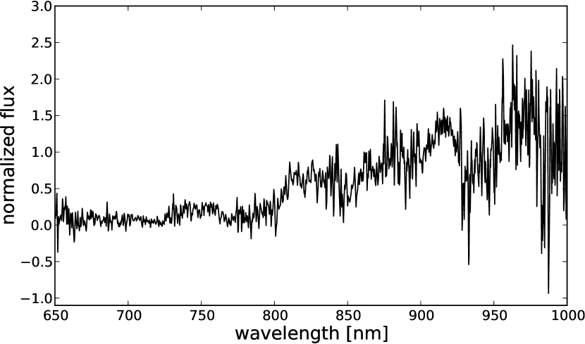
Figure 9: Reduced spectrum of J1458+5436 (SDSS ID 588011216993125015), probably a cool star. Taken with SCORPIO@BTA.

To finally get an impression of the overall performance of our quasar identification approach, we randomly selected three candidates from our result list for spectroscopic follow-up observations in order to confirm their quasar nature and determine their redshift. This very small number of follow-up targets is of course not sufficient to establish an empirical performance of our algorithm in any statistically meaningful sense, but the identification of even one high-z quasar would at least highlight the potential of data mining and machine learning approaches for data-intensive astronomy and also demonstrate a possible way to go with this new branch of astronomy: Since all outcomes of follow-up spectroscopy are valuable for evaluating and optimising a kNN-based classification approach (e.g. sources showing non-quasar spectra can be used to enhance the training set for rejecting contaminating objects such as cool stars), this method would greatly benefit from spectroscopy of a considerable number ($>1000$) of candidate sources.

4.2.1 Observations

The observations were carried out in July 2011 with the SCORPIO instrument at the 6-metre BTA telescope of the Special Astrophysical Observatory on Mt. Pastukhova in southern Russia. A total on-source time of 6.5 hours was spent on three objects that were randomly chosen from our final candidate catalog, only applying a magnitude cut of $i<22.0$ mag in order to obtain reliable spectra in such a short time. To optimise the efficiency of observations, we chose low-resolution grisms GR300R and VPHG550R (a holographic grism) alongside with a wide slit of $2\arcsec$, both resulting in a theoretical spectral resolution of $\sim 40\,\mathrm{\AA}$. Data reduction was done using standard IRAF tasks, including the removal of cosmic rays with lacos-spec. We did not apply an absolute flux calibration since we are only interested in the general shape of the spectrum and its redshift.

4.2.2 Results

From the three observed objects, the brightest one (SDSS ID 587735488676299501) with $i=20.30$ mag turned out to be a cool star even in the very first frames of observations. Therefore, we aborted the run for this object and divided its observation time on the two remaining sources with $i$-band magnitudes of 21.52 mag (SDSS ID 588011218070144145) and 21.45 mag (SDSS ID 588011216993125015), respectively. Figure 8 and 9 show the final wavelangth-calibrated 1D spectra of the objects. As one can clearly see, we have one detection of a quasar with a very pronounced Lyman break at $7,249\,\mathrm{\AA}$ and a broad Lyman $\beta$ emission line at $6,125\,\mathrm{\AA}$ that correspond to a redshift of $\rm{z}\sim 5.0$, regarding errors of the wavelength calibration due to the known flexure of the CCD chip of SCORPIO. The other spectrum is not as easy to classify, therefore we only state that this is not a quasar but most likely another cool star. However, there are classes of objects known, which harbour an AGN without showing distinct signs of AGN-activity in an optical spectrum (Zinn et al., 2011). Therefore we can not make definite statements on the nature of the sources which do not show any signs of AGN-activity in their spectra.

4.2.3 Outlook

We were only able to observe three objects from our final candidate catalog comprising more than 120,000 objects. Since spectroscopy of such faint sources is very time consuming we cannot draw any significant statistical conclusions from these observations regarding the fraction of actual quasars in our catalog. Nevertheless, we point out, that in combination with the excellent agreement with the high-z quasar number densities found in the previous section, the newly identified $\rm{z}\sim 5.0$ quasar is a very promising result. To finally obtain spectra of a substantial number of objects allowing for reliable statistical analysis of our selection approach, many more nights at big telescopes have to be spent.

5 Conclusions

The presented quasar candidate selection approach is highly dependent on the coverage of the feature space induced by the reference samples. Efficient data structures are mandatory to provide good scanning performance when using large reference samples. Except for the last step the kNN retrieval of all other classifiers is accelerated by $k$-d-trees (Bentley, 1975). With the availability of larger spectroscopic surveys and larger sets of known high-z quasars as reference, better photometric selection results will be achievable.

Even though not all of the known quasars are recovered by the presented approach, the resulting candidates have higher probabilities to be a quasar than those found with other approaches. Follow-up observations will help to determine the real detection performance of the candidate selection. The objects that are found not to be quasars will directly improve the reference sets and, thus, the overall detection performance.

References

- Adelman-McCarthy et al. (2008) Adelman-McCarthy J. K., et al. 2008, ApJS, 175, 297
- Antonucci (1993) Antonucci R., 1993, ARA&A, 31, 473
- Bentley (1975) Bentley J. L., 1975, Communications of the ACM, 18, 509
- Bolzonella et al. (2000) Bolzonella M., et al. 2000, A&A, 363, 476
- Boyle et al. (2000) Boyle B. J., et al. 2000, MNRAS, 317, 1014
- Cardamone et al. (2010) Cardamone C. N., et al. 2010, ApJS, 189, 270
- Carlberg (1990) Carlberg R. G., 1990, ApJ, 350, 505
- Cattaneo et al. (2009) Cattaneo A., et al. 2009, Nature, 460, 213
- Cristiani et al. (2004) Cristiani S., et al. 2004, ApJL, 600, L119
- Csabai et al. (2003) Csabai I., et al. 2003, AJ, 125, 580
- Eisenstein et al. (2001) Eisenstein D. J., et al. 2001, AJ, 122, 2267
- Fan et al. (2001) Fan X., et al. 2001, AJ, 122, 2833
- Fan et al. (2003) Fan X., et al. 2003, AJ, 125, 1649
- Fan et al. (2004) Fan X., et al. 2004, AJ, 128, 515
- Fan et al. (2006) Fan X., et al. 2006, AJ, 131, 1203
- Fan (1999) Fan X., 1999, AJ, 117, 2528
- Haiman et al. (1999) Haiman Z., et al. 1999, ApJ, 514, 535
- Haiman & Hui (2001) Haiman Z., Hui L., 2001, ApJ, 547, 27
- Hastie et al. (2009) Hastie T., et al. 2009, The Elements of Statistical Learning: Data Mining, Inference, and Prediction, second edn. Springer, New York, USA
- Kauffmann et al. (2003) Kauffmann G., et al. 2003, MNRAS, 346, 1055
- Komatsu et al. (2011) Komatsu E., et al. 2011, ApJS, 192, 18
- Laurino et al. (2011) Laurino O., et al. 2011, MNRAS, 418, 2165
- Monaco et al. (2000) Monaco P., et al. 2000, MNRAS, 311, 279
- Mortlock et al. (2011) Mortlock D. J., et al. 2011, ArXiv e-prints
- O’Mill et al. (2011) O’Mill A. L., et al. 2011, MNRAS, p. 201
- Richards et al. (2002) Richards G. T., et al. 2002, AJ, 123, 2945
- Schneider et al. (2010) Schneider D. P., et al. 2010, AJ, 139, 2360
- Strauss et al. (2002) Strauss M. A., et al. 2002, AJ, 124, 1810
- Urry & Padovani (1995) Urry C. M., Padovani P., 1995, PASP, 107, 803
- White & Frenk (1991) White S. D. M., Frenk C. S., 1991, ApJ, 379, 52
- Wu & Jia (2010) Wu X., Jia Z., 2010, MNRAS, 406, 1583
- York et al. (2000) York D. G., et al. 2000, AJ, 120, 1579
- Zinn et al. (2011) Zinn P.-C., et al. 2011, A&A, 531, A14