A Multiscale Framework for Challenging Discrete Optimization

Abstract

Current state-of-the-art discrete optimization methods struggle behind when it comes to challenging contrast-enhancing discrete energies (i.e., favoring different labels for neighboring variables). This work suggests a multiscale approach for these challenging problems. Deriving an algebraic representation allows us to coarsen any pair-wise energy using any interpolation in a principled algebraic manner. Furthermore, we propose an energy-aware interpolation operator that efficiently exposes the multiscale landscape of the energy yielding an effective coarse-to-fine optimization scheme. Results on challenging contrast-enhancing energies show significant improvement over state-of-the-art methods.

1 Introduction

We consider discrete pair-wise energies, defined over a (weighted) graph $\left(\mbox{$\mathcal{V}$},\mbox{$\mathcal{E}$}\right)$:

$$E\left(L\right) = \sum_{i\in\mbox{$\mathcal{V}$}}\varphi_{i}\left(l_{i}\right)+\sum_{\left(i,j\right)\in\mbox{$\mathcal{E}$}}w_{ij}\cdot\varphi\left(l_{i},l_{j}\right)$$ (1)

where $\mathcal{V}$ is the set of variables and $\mathcal{E}$ is the set of edges. The sought solution is a discrete vector: $L\in\left\{1,\ldots,l\right\}^{n}$, with $n$ variables each taking one of $l$ possible labels, minimizing (1).

Most energy instances of form (1) considered in the literature are smoothness preserving: that is, assigning neighboring variables to the same label costs less energy. Smoothness preserving energies include submodular [15], metric and semi-metric [4] energies. State-of-the-art optimization algorithms (e.g., TRW-S [11], large move [4] and dual decomposition (DD) [13]) handle smoothness preserving energies well yielding close to optimal results. However, when it comes to contrast-enhancing energies (i.e., favoring different labels for neighboring variables) existing algorithms provide poor approximations (see e.g., [17, example 8.1], [11, §5.1]). For contrast-enhancing energies the relaxation of TRW and DD is no longer tight and therefore they converge to a far from optimal solution.

This work suggests a multiscale approach to the optimization of contrast-enhancing energies. Coarse-to-fine exploration of the solution space allows us to effectively avoid getting stuck in local minima. Our work makes two major contributions: (i) An algebraic representation of the energy allows for a principled derivation of the coarse scale energy using any linear coarse-to-fine interpolation. (ii) An energy-aware method for computing the interpolation operator which efficiently exposes the multiscale landscape of the energy.

Multiscale approaches for discrete optimization has been proposed in the past (e.g., [7, 14, 6, 10, 12, 9]). However, they focus mainly on accelerating the optimization process of smoothness preserving energies. Furthermore, these methods are usually restricted to a diadic coarsening of grid-based energies, and suggest “ad-hoc” and heuristic derivation of the coarse-scale energy (e.g., [10, §3]). In contrast, our framework suggests a principled derivation of coarse scale energy using a novel energy-aware interpolation yielding low energy solutions.

2 Multiscale Energy Pyramid

Our algebraic representation requires the substitution of vector $L$ in (1) with an equivalent binary matrix representation $U\in\left\{0,1\right\}^{n\times l}$. The rows of $U$ correspond to the variables, and the columns corresponds to labels: $U_{i,\alpha}=1$ iff variable $i$ is labeled “$\alpha$” ($l_{i}=\alpha$). Expressing the energy (1) using $U$ yields a quadratic representation:

$$E\left(U\right) = Tr\left(DU^{T}+WUVU^{T}\right)$$ (2)

s.t. $$U\in\left\{0,1\right\}^{n\times l},\ \sum_{\alpha=1}^{l}U_{i\alpha}=1$$ (3)

where $W=\left\{w_{ij}\right\}$, $D\in\mathbb{R}^{n\times l}$ s.t. $D_{i,\alpha}\mbox{$\stackrel{{\scriptstyle\mbox{{def}}}}{{=}}$}\varphi_{i}(\alpha)$, and $V\in\mathbb{R}^{l\times l}$ s.t. $V_{\alpha,\beta}\mbox{$\stackrel{{\scriptstyle\mbox{{def}}}}{{=}}$}\varphi\left(\alpha,\beta\right)$, $\alpha,\beta\in\left\{1,\ldots,l\right\}$. An energy over $n$ variables with $l$ labels is now parameterized by $\left(n,l,D,W,V\right)$.

Let $\left(n^{f},l,D^{f},W^{f},V\right)$ be the fine scale energy. We wish to generate a coarser representation $\left(n^{c},l,D^{c},W^{c},V\right)$ with fewer variables $n^{c}<n^{f}$. This representation approximates $E\left(U^{f}\right)$ using fewer variables: $U^{c}$ with only $n^{c}$ rows.

An interpolation matrix $P\in\left[0,1\right]^{{n^{f}}\times{n^{c}}}$ s.t. $\sum_{j}P_{ij}=1$ $\forall i$, maps coarse assignment $U^{c}$ to fine assignment $PU^{c}$. For any fine assignment that can be approximated by a coarse assignment $U^{c}$, i.e., $U^{f}=PU^{c}$, we can write eq. (2):

$$E\left(U^{f}\right) = Tr\left(D^{f}{U^{f}}^{T}+W^{f}U^{f}V{U^{f}}^{T}\right)=Tr\left(D^{f}{U^{c}}^{T}P^{T}+W^{f}PU^{c}V{U^{c}}^{T}P^{T}\right)$$

$$= Tr\Big{(}\underbrace{\left(P^{T}D^{f}\right)}_{\mbox{$\mbox{$\stackrel{{\scriptstyle\mbox{{def}}}}{{=}}$}D^{c}$ }}{U^{c}}^{T}+\underbrace{\left(P^{T}W^{f}P\right)}_{\mbox{$\mbox{$\stackrel{{\scriptstyle\mbox{{def}}}}{{=}}$}W^{c}$}}U^{c}V{U^{c}}^{T}\Big{)}=Tr\left(D^{c}{U^{c}}^{T}+W^{c}U^{c}V{U^{c}}^{T}\right)$$

$$= E\left(U^{c}\right)$$

We have generated a coarse energy $E\left(U^{c}\right)$ parameterized by $\left(n^{c},l,D^{c},W^{c},V\right)$ that approximates the fine energy $E(U^{f})$. This coarse energy is of the same form as the original energy allowing us to apply the coarsening procedure recursively to construct an energy pyramid.

Our principled algebraic representation allows us to perform label coarsening in a similar manner. Looking at a different interpolation matrix $\hat{P}\in\left[0,1\right]^{\mbox{$l^{f}\times l^{c}$}}$, we interpolate a coarse solution by $U^{\hat{f}}\leftarrow U^{\hat{c}}\hat{P}^{T}$. This time the interpolation matrix $\hat{P}$ acts on the labels, i.e., the columns of $U$. The coarse labeling matrix $U^{\hat{c}}$ has the same number of rows (variables), but fewer columns (labels). Coarsening the labels yields:

$$E\left(U^{\hat{c}}\right)=Tr\left(\left(D^{\hat{f}}\hat{P}\right)\mbox{$U^{\hat{c}}$}^{T}+WU^{\hat{c}}\left(\hat{P}^{T}V^{\hat{f}}\hat{P}\right)\mbox{$U^{\hat{c}}$}^{T}\right)$$ (5)

Again, we end up with the same type of energy, but this time it is defined over a smaller number of discrete labels: $\left(n,l^{c},D^{\hat{c}},W,V^{\hat{c}}\right)$, where $D^{\hat{c}}\mbox{$\stackrel{{\scriptstyle\mbox{{def}}}}{{=}}$}D^{\hat{f}}\hat{P}$ and $V^{\hat{c}}\mbox{$\stackrel{{\scriptstyle\mbox{{def}}}}{{=}}$}\hat{P}^{T}V^{\hat{f}}\hat{P}$.

Equations (2) and (5) encapsulate one of our key contributions: Constructing an energy pyramid depends only on $P$. For any interpolation $P$ it is straightforward to derive the coarse-scale energy in a principled manner. But what is an appropriate interpolation?

3 Energy-aware Interpolation

The effectiveness of the multiscale approximation of (2) and (5) heavily depends on the interpolation matrix $P$ ($\hat{P}$ resp.). The matrix $P$ can be interpreted as an operator that aggregates fine-scale variables into coarse ones (Fig. 1). Aggregating fine variables $i$ and $j$ into a coarser one excludes from the search space all assignments for which $l_{i}\neq l_{j}$. This aggregation is undesired if assigning $i$ and $j$ to different labels yields low energy. However, when variables $i$ and $j$ are in agreement under the energy (i.e., assignments with $l_{i}=l_{j}$ yield low energy), aggregating them together allows for efficient exploration of low energy assignments. A desired interpolation aggregates $i$ and $j$ when $i$ and $j$ are in agreement under the energy.

[r][r]

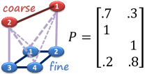
Figure 1: Interpolation as soft variable aggregation: fine variables 1, 2, 3 and 4 are softly aggregated into coarse variables 1 and 2. For example, fine variable 1 is a convex combination of $.7$ of 1 and $.3$ of 2. Hard aggregation is a special case where $P$ is a binary matrix. In that case each fine variable is influenced by exactly one coarse variable.

To estimate these agreements we empirically generate several samples with relatively low energy, and measure the label agreement between neighboring variables $i$ and $j$ in these samples. We use Iterated Conditional Modes (ICM) [3] to obtain locally low energy assignments. This procedure may be interpreted as Gibbs sampling from the Gibbs distribution $p\left(U\right)\propto\exp\left(-\frac{1}{T}E\left(U\right)\right)$ at the limit $T\rightarrow 0$ (i.e., the “zero-temperature” limit). Performing $t=10$ ICM iterations with $K=10$ random restarts provides us with $K$ samples $\left\{L^{k}\right\}_{k=1}^{K}$. The disagreement between neighboring variable $i$ and $j$ is estimated as $d_{ij}=\frac{1}{K}\sum_{k}V_{l^{k}_{i},l^{k}_{j}}$, where $l^{k}_{i}$ is the label of variable $i$ in the $k^{th}$ sample. Their agreement is then given by $c_{ij}=\exp\left(-\frac{d_{ij}}{\sigma}\right)$, with $\sigma\propto\max V$.

Using the variable agreements, $c_{ij}$, we follow the Algebraic Multigrid (AMG) method of [5] to first determine the set of coarse scale variables and then construct an interpolation matrix $P$ that softly aggregates fine scale variables according to their agreement with the coarse ones.

We begin by selecting a set of coarse representative variables $\mbox{$\mathcal{V}$}^{c}\subset\mbox{$\mathcal{V}$}^{f}$, such that every variable in $\mbox{$\mathcal{V}$}^{f}\backslash\mbox{$\mathcal{V}$}^{c}$ is in agreement with $\mbox{$\mathcal{V}$}^{c}$. A variable $i$ is considered in agreement with $\mbox{$\mathcal{V}$}^{c}$ if $\sum_{j\in\mbox{$\mathcal{V}$}^{c}}c_{ij}\geq\beta\sum_{j\in\mbox{$\mathcal{V}$}^{f}}c_{ij}$. That is, every variable in $\mbox{$\mathcal{V}$}^{f}$ is either in $\mbox{$\mathcal{V}$}^{c}$ or is in agreement with other variables in $\mbox{$\mathcal{V}$}^{c}$, and thus well represented in the coarse scale.

We perform this selection greedily and sequentially, starting with $\mbox{$\mathcal{V}$}^{c}=\emptyset$ adding $i$ to $\mbox{$\mathcal{V}$}^{c}$ if it is not yet in agreement with $\mbox{$\mathcal{V}$}^{c}$. The parameter $\beta$ affects the coarsening rate, i.e., the ratio $n^{c}/n^{f}$, smaller $\beta$ results in a lower ratio.

At the end of this process we have a set of coarse representatives $\mbox{$\mathcal{V}$}^{c}$. The interpolation matrix $P$ is then defined by:

$$P_{iI(j)}=\left\{\begin{array}[]{cl}c_{ij}&i\in\mbox{$\mathcal{V}$}^{f}\backslash\mbox{$\mathcal{V}$}^{c},\ j\in\mbox{$\mathcal{V}$}^{c}\\ 1&i\in\mbox{$\mathcal{V}$}^{c},j=i\\ 0&\mbox{otherwise}\\ \end{array}\right.$$ (6)

Where $I(j)$ is the coarse index of the variable whose fine index is $j$ (in Fig. 1: $I(2)=1$ and $I(3)=2$).

We further prune rows of $P$ leaving only $\delta$ maximal entries. Each row is then normalized to sum to 1. Throughout our experiments we use $\beta=0.2$ and $\delta=3$ for computing $P$.

4 A Unified Discrete Multiscale Framework

Given an energy $\left(n,l,D,W,V\right)$ at scale $s=0$, our framework first works fine-to-coarse to compute interpolation matrices $\left\{P^{s}\right\}$ that construct the “energy pyramid”: $\left\{\left(n^{s},l,D^{s},W^{s},V\right)\right\}_{s=0,\ldots,S}$. Typically we reduce the number of variables by a factor of $2$ between consecutive levels, resulting with less than $10$ variables at the coarsest scale. Since there are very few degrees of freedom at the coarsest scale ICM is likely to obtain a low-energy coarse solution. Then, at each scale $s$ the coarse solution $U^{s}$ is interpolated to a finer scale $s-1$: $\tilde{U}^{s-1}\leftarrow P^{s}U^{s}$. At the finer scale $\tilde{U}^{s-1}$ serves as a good initialization for ICM (fractional solutions are rounded). These two steps of interpolation followed by refinement are repeated for all scales from coarse to fine.

Our energy-aware interpolation and ICM play complementary roles in this multiscale framework. ICM makes fine scale local refinements of a given labeling, while the energy-aware interpolation makes coarse grouping of variables to expose global behavior of the energy. In a sense, ICM is a discrete equivalent to the continuous Gauss-Seidel relaxation used in continuous domain multiscale schemes.

5 Experimental Results

We evaluated our multiscale framework on challenging contrast enhancing synthetic, as well as on co-clustering energies. We follow the protocol of [16] that uses the lower bound as a baseline for comparing performance of different optimization methods on different energies. We report the ratio between the resulting energy and the lower bound (in percents), closer to $100\%$ is better.

Table 1: Synthetic results: Showing percent of achieved energy value relative to the lower bound computed by TRW-S (closer to $100\%$ is better) for ICM and TRW-S for varying strengths of the pair-wise term ($\lambda=5,10,15$, stronger $\rightarrow$ harder to optimize.)

$\lambda$	ICM		TRW-S
	Ours	single scale
$5$	$112.6\%$	$115.9\%$	$116.6\%$
$10$	$123.6\%$	$130.2\%$	$134.6\%$
$15$	$127.1\%$	$135.8\%$	$138.3\%$

Table 2: Co-clustering results: Baseline for comparison are state-of-the-art results of [8]. (a) We report our results as percent of the baseline: smaller is better, lower than $100\%$ even outperforms state-of-the-art. (b) We also report the fraction of energies for which our multiscale framework outperform state-of-the-art.

	ICM		TRW-S
	Ours	single scale
(a)	$99.9\%$	$177.7\%$	$176.2\%$
(b)	$55.6\%$	$0.0\%$	$0.5\%$

Synthetic:  We begin with synthetic contrast-enhancing energies defined over a 4-connected grid graph of size $50\times 50$ ($n=2500$), and $l=5$ labels. The unary term $D\sim\mathcal{N}\left(0,1\right)$. The pair-wise term $V_{\alpha\beta}=V_{\beta\alpha}\sim\mathcal{U}\left(0,1\right)$ ($V_{\alpha\alpha}=0$) and $w_{ij}=w_{ji}\sim\lambda\cdot\mathcal{U}\left(-1,1\right)$. The parameter $\lambda$ controls the relative strength of the pair-wise term, stronger (i.e., larger $\lambda$) results with energies more difficult to optimize (see [11]). The resulting synthetic energies are contrast-enhancing (since $w_{ij}$ may become negative). Table 2 shows results, averaged over 100 experiments. Using our multiscale framework to perform coarse-to-fine optimization of the energy yields significantly lower energies than single-scale methods used (ICM and TRW-S).

Co-clustering (Correlation-Clustering):  The problem of co-clustering addresses the matching of superpixels within and across frames in a video sequence. Following [2, §6.2], we treat co-clustering as a minimization of a discrete Potts energy adaptively adjusting the number of labels. The resulting energies are contrast-enhancing (with some $w_{ij}<0$), have no underlying regular grid, no data term, and are very challenging to optimize. We obtained 77 co-clustering energies, courtesy of [8], used in their experiments. Table 2 compares our discrete multiscale framework to the state-of-the-art results of [8] obtained by applying specially tailored convex relaxation method. Our multiscale framework improves state-of-the-art for this family of challenging energies and significantly outperforms TRW-S.

6 Extensions

It is rather straightforward to extend our framework to handle energies with different $V$ for every pair $(i,j)$. Moreover, higher order potentials can also be considered using the same algebraic representation. A detailed derivation may be found in [1].

Acknowledgments

We would like to thank Irad Yavneh, Maria Zontak and Daniel Glasner for their insightful remarks and discussions. Special thanks go to Michal Irani for her exceptional encouragement and support.

References

- [1] S. Bagon. Discrete Energy Minimization, beyond Submodular: Applications and Approximations. PhD thesis, Weizmann Institute of Science, http://arxiv.org/abs/1210.7362, 2012.
- [2] S. Bagon and M. Galun. Large scale correlation clustering optimization. arXiv, 2011.
- [3] J. Besag. On the statistical analysis of dirty pictures. Journal of the Royal Statistical Society, 1986.
- [4] Y. Boykov, O. Veksler, and R. Zabih. Fast approximate energy minimization via graph cuts. PAMI, 2002.
- [5] A. Brandt. Algebraic multigrid theory: The symmetric case. Applied Mathematics and Computation, 1986.
- [6] P. Felzenszwalb and D. Huttenlocher. Efficient belief propagation for early vision. IJCV, 2006.
- [7] B. Gidas. A renormalization group approach to image processing problems. PAMI, 1989.
- [8] D. Glasner, S. N. Vitaladevuni, and R. Basri. Contour-based joint clustering of multiple segmentations. In CVPR, 2011.
- [9] T. Kim, S. Nowozin, P. Kohli, and C. Yoo. Variable grouping for energy minimization. In CVPR, 2011.
- [10] P. Kohli, V. Lempitsky, and C. Rother. Uncertainty driven multiscale optimization. In DAGM, 2010.
- [11] V. Kolmogorov. Convergent tree-reweighted message passing for energy minimization. PAMI, 2006.
- [12] N. Komodakis. Towards more efficient and effective LP-based algorithms for MRF optimization. In ECCV, 2010.
- [13] N. Komodakis, N. Paragios, and G. Tziritas. MRF energy minimization and beyond via dual decomposition. PAMI, 2011.
- [14] P. Pérez and F. Heitz. Restriction of a markov random field on a graph and multiresolution statistical image modeling. IEEE Tran. on Inf. Theory, 1996.
- [15] D. Schlesinger and B. Flach. Transforming an arbitrary minsum problem into a binary one. Technical report, TU, Fak. Informatik, 2006.
- [16] R. Szeliski, R. Zabih, D. Scharstein, O. Veksler, V. Kolmogorov, A. Agarwala, M. Tappen, and C. Rother. A comparative study of energy minimization methods for markov random fields with smoothness-based priors. PAMI, 2008.
- [17] M. Wainwright, T. Jaakkola, and A. Willsky. MAP estimation via agreement on trees: message-passing and linear programming. Information Theory, IEEE Transactions on, 2005.