A critical assessment of two-body and three-body interactions in water

Abstract

The microscopic behavior of water under different conditions and in different environments remains the subject of intense debate. A great number of the controversies arises due to the contradictory predictions obtained within different theoretical models. Relative to conclusions derived from force fields or density functional theory, there is comparably less room to dispute highly-correlated electronic structure calculations. Unfortunately, such ab initio calculations are severely limited by system size. In this study, a detailed analysis of the two- and three-body water interactions evaluated at the CCSD(T) level is carried out to quantitatively assess the accuracy of several force fields, density functional theory, and ab initio-based interaction potentials that are commonly used in molecular simulations. Based on this analysis, a new model, HBB2-pol, is introduced which is capable of accurately mapping CCSD(T) results for water dimers and trimers into an efficient analytical function. The accuracy of HBB2-pol is further established through comparison with the experimentally determined second and third virial coefficients.

I Introduction

Connecting small clusters of water and the condensed phases of water through a single molecular model has been a long sought-after but so-far unachieved goal. The challenges involved in the pursuit of this goal are numerous. For example, at the cluster level, the Born-Oppenheimer energies of topologically distinct isomers of the water hexamer differ by less than 1 kcal/mol Dahlke et al. (2008); Bates and Tschumper (2009); Góra et al. (2011), indicating that highly-correlated electronic structure calculations are required to quantitatively determine the energy order of these isomers. In this regard, a faithful description of molecular flexibility appears to be particularly important.Góra et al. (2011) Furthermore, it has also been shown that nuclear quantum-mechanical effects can impact the structural, thermodynamic, and dynamical properties of both clusters and bulk phases of water.Soper and Benmore (2008); Paesani and Voth (2009); Wang et al. (2012); Markland and Berne (2012) The explicit inclusion of nuclear quantum effects in simulations exacerbates the computational expense of a model, providing additional strain on the ability to obtain statistically meaningful results.

The majority of water simulations rely on force fields, which are built upon the many-body expansion of the interaction energy,Hankins et al. (1970)

$$E (1,\dots,N)=\sum_{i}^{N}V^{1B}(i)+\sum_{i<j}^{N}V^{2B}(i,j)$$

$$+\sum_{i<j<k}^{N}V^{3B}(i,j,k)+\dots+V^{NB}(1,\dots,N).$$ (1)

Here, $V^{1B}(i)=E(i)-E_{eq}(i)$ is the one-body (1B) potential, which describes the energy required to deform an individual molecule from its equilibrium geometry. In common force-fields, the 1B interactions include all bonded terms (i.e., stretches, bends, and torsions). For systems, such as water, that are easily reduced to distinct molecules, a 1B configuration is typically referred to as a “monomer”, and groups of 2, 3, … , $N$ interacting monomers are then termed “dimers”, “trimers”, …, “$N$-mers”. In Eq. I, higher-order interactions are defined recursively through the lower-order terms. For instance, the two-body (2B) interaction is expressed as

$$V^{2B}=E(1,2)-\sum_{i=1}^{2}E(i)$$

where $E(1,2)$ is the dimer energy. Similarly, the three-body (3B) interaction is

$$V^{3B}=E(1,2,3)-\sum_{i<j}^{3}E(i,j)+\sum_{i=1}^{3}E(i)$$

with $E(1,2,3)$ being the trimer energy. Common force fields are pairwise additive, meaning that three-body and higher interactions are neglected.

If it converges quickly, the many-body expansion represents a powerful approach to studying condensed phases as it allows for the energy of an $N$-molecule system to be expressed as a sum of lower-order interactions that can in principle be calculated with high accuracy. Recently, a detailed study of the convergence of the many-body expansion for water based on the analysis of small clusters was performed using coupled cluster theory with single, double, and perturbative triple excitations [CCSD(T)] and large basis sets.Góra et al. (2011) Consistent with previous observations Xantheas (1994, 2000); Defusco et al. (2007); Kumar et al. (2010); Hodges et al. (1997); Ojamie and Hermansson (1994); Pedulla et al. (1996); Cui et al. (2006), it was determined that, although two-body interactions dominate the expansion, the three-body term can contribute up to 30% of the total energy of the water hexamer. An estimate of the relative magnitudes of the many-body terms in liquid was obtained through an RIMP2 analysis of the 21-mer, for which two-body interactions were found to contribute 75-80% of the total interaction energy and three-body interactions comprised 15-20%.Cui et al. (2006) For both the water hexamer and the 21-mer, higher-order terms contribute less than 5% of the total interaction energy. It should be noted that, while quickly converging for water, the many-body expansion has been shown to converge slowly and with marked oscillatory behavior for other systems.Hermann et al. (2007)

In this study, the accuracy of several force fields, density functional theory (DFT), and ab initio potentials in reproducing the two- and three-body water interactions is assessed through a detailed comparison with data obtained at the CCSD(T) level of theory (Section II). Based on this analysis, a new ab initio water model, HBB2-pol, is then introduced in Section III. In Section IV, we show that HBB2-pol accurately maps the CCSD(T) results for both the 2B and 3B interactions into an efficient analytical functional form and predicts the second and third virial coefficients in excellent agreement with the available experimental data. A summary is given in Section V.

II Analysis of two- and three-body water interactions

II.1 Water models

The many-body expansion provides the underlying basis for common classical force fields. In most cases, including the widely-used TIP4P and SPC familiesJorgensen et al. (1983); Berendsen et al. (1981), pairwise additivity is assumed, with three- and higher-body interactions being “encoded” into the effective two-body contributions. In addition, the majority of these models treat the water molecules as rigid monomers (i.e., the 1B interactions are set to zero), with only few quantum water models, notably as q-TIP4P/f and qSPC/Fw,Habershon et al. (2009); Paesani et al. (2006) allowing for molecular flexibility. Nevertheless, pairwise force fields have been surprisingly successful at reproducing, at least qualitatively, the properties of water in homogeneous environments.Vega and Abascal (2011) However, such force fields are expected to be inherently limited in their ability to model the microscopic behavior of aqueous interfaces, water confined at the nanoscale, and clusters, whose properties are sensitive to the detailed interplay of 1B, 2B, 3B, and higher-body interactions.Xantheas (1994, 2000); Defusco et al. (2007); Kumar et al. (2010); Hodges et al. (1997); Ojamie and Hermansson (1994); Pedulla et al. (1996); Cui et al. (2006)

Recent work has focused on improving empirical models through inclusion of three-body interactions, leading to the development of the E3B model.Kumar and Skinner (2008); Tainter et al. (2011) Although the inclusion of explicit 3B interactions greatly improves the accuracy of the E3B model relative to pairwise force fields, the use of rigid water monomers and empirical parameterization necessarily misses some of the fundamental properties of the many-body expansion. For example, recent E3B simulations of the isomeric equilibria of the water hexamer have led to predictions that are markedly different from ab initio calculations. Specifically, the prism structure, which corresponds to the energetically lowest-lying isomer at the MP2 and CCSD(T) levels of theory, Góra et al. (2011); Bates and Tschumper (2009) is unstable in the E3B calculations.Tainter and Skinner (2012)

Since non-pairwise additive intermolecular interactions arise primarily from electronic polarization at long distances, several methods have been proposed to incorporate this effect into the framework of classical force fields.Lopes et al. (2009) One common approach is the Applequist polarizable point dipole model,Applequist et al. (1972) which was elaborated upon by Thole to address the so-called polarization catastrophe.Thole (1981) Thole-type polarizable force fields for water include TTM3-FFanourgakis and Xantheas (2008), TTM4-FBurnham et al. (2008), and AMOEBARen and Ponder (2003) models.

Among methods that attempt to solve directly the many-body problem from “first principles”, semiempirical models represent an attractive alternative due to their computational efficiency. Semiempirical models such as PM3Stewart (1989) and PM3-MAISBernal-Uruchurtu and Ruiz-López (2000) were derived within the MNDO scheme and differ primarily in the form of the core-core repulsion as well as in the precise values of their adjustable parameters. These models were parametrized either by fitting experimental data for a wide variety of systems (PM3) or ab initio reference data in the case of PM3-MAIS. Due to the use of a minimal basis and the explicit neglect of correlation, semiempirical methods are particularly limited in their ability to describe non-bonded interactions. This deficiency has been addressed by the SCP-NDDO model, which augments traditional semiempirical methods with classical polarization.Chang et al. (2008) SCP-NDDO has shown success in modeling water clusters and has recently been extended to simulations of bulk properties.Murdachaew et al. (2011)

Different DFT methods has also been extensively used to the study of condensed phases, primarily through the use of GGA functionals such as BLYPBecke (1988); Lee et al. (1988) and PBE.Perdew et al. (1996) However, common density functionals are by construction limited in their ability to describe weakly interacting van der Waals complexes. One attempt to address this problem involves the addition of a dispersion correction to the energy through the ${C_{6}}\big{/}{R^{6}}$ term, where the $C_{6}$ parameters are atom and basis-set specific Grimme (2004, 2006). These “DFT-D” models have successfully described systems such as the solvation of iodide in water Fulton et al. (2010), but are limited by the need to develop parameters for each functional/basis set.Ma et al. (2012) Furthermore, because the correction is pairwise additive, it neglects higher-body dispersion contributions. Recent work to address this limitation has been reported.Grimme et al. (2010)

A promising alternative to the pairwise DFT-D correction is represented by the non-local van der Waals (nl-vdW) functionals.Dion et al. (2004); Lee et al. (2010); Vydrov and Van Voorhis (2010) These nl-vdW functionals utilize the electron density to define a non-local correlation contribution to the exchange-correlation functional, leading to a consistent description of both short-range and long-range interactions. Since no atomic or basis-set dependent parameters are required to describe the dispersion interaction due to the explicit dependence of the non-local correlation on the electron density, nl-vdW functionals, in principle, require minimal parameterization and are system-independent. In practice, great care must be taken to avoid double counting of correlation effects in the combination of semi-local and non-local terms. Van der Waals density functionals have recently been applied to the study of liquid waterWang et al. (2011) and iceMurray and Galli (2012).

One final class of models is represented by the ab initio-based interaction potentials. These models are built upon a rigorous treatment of the many-body expansion of interactions and are characterized by having a functional form that is sufficiently flexible to accurately map high-quality ab initio reference data. Examples of such models are DPP2,Kumar et al. (2010) CC-pol, Bukowski et al. (2008, 2008) and WHBB.Wang et al. (2011) DPP2 and CC-pol are restricted to the rigid, vibrationally averaged monomer geometries, while WHBB uses permutationally invariant polynomials to represent the flexible monomer 2B and 3B potential energy surfaces (PESs). Such ab initio-based interaction potentials are quite computationally demanding and are most commonly used in calculations for gas phase systemsWang et al. (2012), although bulk properties have been obtained from classical simulations with CC-polBukowski et al. (2008, 2007) and DPP2 Kumar et al. (2010). Very recently, a flexible version of CC-pol has been developed, CC-pol-8sf, and the effects of flexibility on the dimer vibrational-rotation-tunneling (VRT) spectra have been characterized.Leforestier et al. (2012) It was found that both CC-pol-8sf and HBB2 (the 2B potential of WHBB) reproduce the experimental VRT spectra “about equally well”.Leforestier et al. (2012)

II.2 Comparison to CCSD(T)

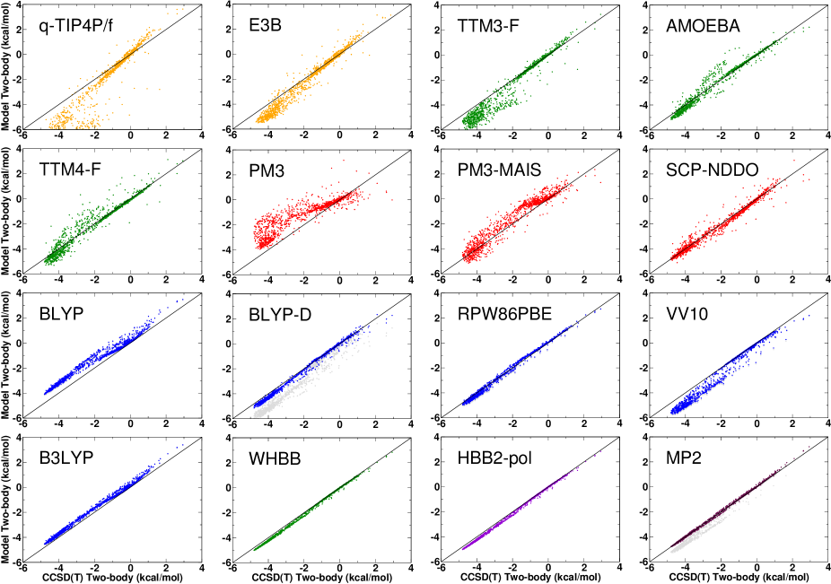
Figure 1: Correlation plots for the 2B interactions. Plotted on the x-axes is the BSSE-corrected CCSD(T)/aug-cc-pVTZ energies. On the y-axes are the energies for each model. Empirically parametrized models are in orange, polarizable models in green, semiempirical methods in red, DFT methods in blue, and MP2 in maroon. For DFT and MP2, the colored dots are BSSE-corrected energies, while gray dots are BSSE-uncorrected energies. The new ab initio-based model, HBB2-pol, is in violet.

Here, we assess the ability of the models presented in Section II.1 to describe the 2B and 3B water interactions. Roughly 1400 2B interactions and 500 3B interactions were evaluated at the CCSD(T)/aug-cc-pVTZ levelRaghavachari et al. (1989); Dunning (1989) and corrected for the basis set superposition error (BSSE) using the counterpoise method.Boys and Bernardi (1970) These (flexible) molecular configurations were extracted from 1) classical molecular dynamics (MD) simulations of hexamers at T $\leq$ 30 K using the WHBB potential, 2) classical MD simulations of ice I${}_{\text{h}}$ carried out with TTM3-F at 50 K, and 3) classical MD simulations of bulk water at 298 K and experimental density using TTM3-F. Hereafter, these configurations are referred to as “low-energy” configurations. For the analysis of E3B, the CCSD(T) reference interaction energies were recomputed for “rigidified” molecules corresponding to the flexible configurations that were used in the comparison of the other models. All DFT energies were computed using the aug-def2-TZVPP basisDunning (1989); Weigend and Ahlrichs (2005) with the exception of BLYP-D, for which the TZVPP basis was used as in the original parametrization of the model.Schafer et al. (1994); Grimme (2004, 2006) MP2 energies were computed with the aug-cc-pVTZ basis, and both DFT and MP2 interactions were corrected for BSSE. All ab initio calculations were performed using the freely-available ab initio package ORCAWennmohs and Neese (2008). PM3 and PM3-MAIS energies were calculated using the AMBER/SQM semi-empirical packageWalker et al. (2008), while the SCP-NDDO energies were obtained using CP2K.cp (2); Murdachaew et al. (2011) A linear regression analysis for the data presented in Figures 1 and 2, as well as root mean square error with respect to CCSD(T) data, are presented in the supporting material.

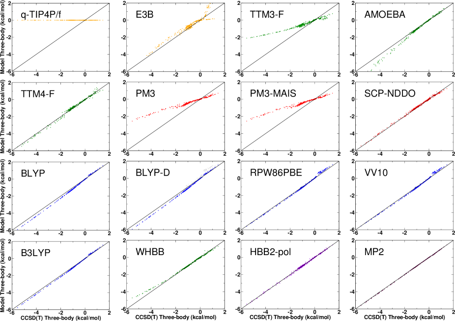
Figure 2: Correlation plots for the 3B interactions. Plotted on the x-axes is the CCSD(T)/aug-cc-pVTZ energies corrected for BSSE. On the y-axes are the 3B energies for each model. The color scheme is the same as in Figure 1.

Figures 1 and 2 show correlation plots for the 2B and 3B interactions calculated for all models described in Section II.1 relative to the CCSD(T)/aug-cc-pVTZ energies. While most empirical pairwise force fields implicitly include nuclear quantum effects, models such as q-TIP4P/f and q-SPC/Fw were specifically parameterized for quantum simulations and, therefore, presumably provide an approximation to the actual Born-Oppenheimer PES.Habershon et al. (2009); Paesani et al. (2006) As can be seen from Figure 1, q-TIP4P/f deviates substantially from the CCSD(T) 2B potential energy surface to compensate for the neglect of higher-order interactions (Figure 2). Force fields that account for higher-order terms generally provide a more accurate description of the 2B interactions than effective pairwise models. In this context, while E3B and TTM3-F/TTM4-F/AMOEBA treat higher-order interactions using different schemes, all four models give 2B interactions that are in closer agreement with the CCSD(T) results than the effective pairwise models. It is interesting to note that E3B, which does not not explicitly include induction and was not parameterized using ab initio data, describes the 3B contributions energies reasonably well.

The three polarizable models considered in this study (TTM3-F, TTM4-F, and AMOEBA) differ in the way they describe the variation of the molecular charge distribution. As an isolated monomer deforms, the molecular dipole moment varies in a “nonlinear” fashion with respect to the intramolecular coordinates, resulting in a “nonlinear dipole moment surface” (DMS).Burnham and Xantheas (2002) In TTM4-F, the first-order changes of the DMS are fit to electric multipoles and polarizabilites calculated at the MP2 level. The intramolecular dependence of the atomic charges in TTM3-F was instead motivated by the observation that, while the gas phase monomer charges decrease during the homolytic dissociation, a water molecule in the condensed phase dissociates into charged ions. This argument was used to justify an empirical correction to ab initio-derived values, giving rise to effective charges that increase as the monomer geometry departs from equilibrium. By contrast, although AMOEBA takes into account intramolecular flexibility, the monomer charges are geometry independent.Ren and Ponder (2003) Interestingly, while the accurate monomer DMS has been reported to be essential to reproducing the solvated monomer geometry,Burnham and Xantheas (2002) the three-body interaction of AMOEBA is only slightly less accurate than TTM4-F, with RMS errors of 0.22 and 0.09 kcal/mol respectively. It is also important to mention that, unlike in TTM3-F, in both AMOEBA and TTM4-F the molecular polarzability is anisotropic. It is unclear whether the inaccuracy observed in the TTM3-F 3B energies arises from its use of effective charges, isotropic molecular polarizability or both.

Among the semiempirical methods, PM3 was fitted to a wide range of experimental and ab initio data, while PM3-MAIS and SCP-NDDO were both fitted to ab initio reference data of water clusters. It is therefore not surprising that the 2B interactions of PM3-MAIS and SCP-NDDO are in better agreement with the CCSD(T) data than PM3. It is interesting, however, that SCP-NDDO shows much tighter correlation to the ab initio data than PM3-MAIS, even though the latter uses almost twice as many adjustable parameters as SCP-NDDO. While the two MNDO-type semiempirical methods display significant deficiencies in describing the 3B interactions, SCP-NDDO reproduces the CCSD(T) data quite accurately. These results suggest that the addition of classical polarization, as implemented in SCP-NDDO, can allow semiempirical methods to accurately describe intermolecular interactions without requiring extensive reparametrizations of the core-core terms.

At the 2B level, the GGA density functionals differ appreciably from the CCSD(T) results (see Supporting Information for PBE and PBE0 results), with BLYP systematically underestimating the interaction strength. The inclusion of the dispersion correction in BLYP-D improves the agreement with the CCSD(T) values for the 2B interactions. However, although DFT is less sensitive to basis set incompleteness than wavefunction methods, the absence of diffuse functions in the BLYP-D basis results in a large BSSE correction (see figure 1, where blue circles give the BSSE-corrected interaction and gray circles the BSSE-uncorrected interaction). Indeed, BSSE is so small for BLYP, B3LYP, RPW86PBE, and VV10 that it is barely visible in Figures 1 and 2. While BLYP-D can accurately describe the 2B interactions when a sufficiently large basis set is used or the energy values are corrected for BSSE, how to balance these factors in condensed phase simulations is not straightforward and is the subject of ongoing research.VandeVondele and Hutter (2007); Ma et al. (2012)

While the use of hybrid functionals, such as B3LYP Becke (1993); Stephens et al. (1994), results in a much tighter correlation to the CCSD(T) data than GGA functionals, B3LYP nonetheless inherently suffers from inadequate treatment of dispersion interactions, which leads to an incorrect long-range behavior.Klimes and Michaelides (2012) Among recent nl-vdW functionals, VV10 appears to over-correct its parent functional, RPW86PBE, leading to over bound 2B interactions. All DFT methods perform reasonably well for the 3B interactions. It is important to note that, because the dispersion correction is pair additive, BLYP and BLYP-D provide identical 3B interactions. By contrast, nl-vdW functionals include a three-body dispersion correction, although this is almost negligible for VV10 (see Supporting Information). MP2 agrees well with CCSD(T), with an RMS of 0.03 and 0.02 kcal/mol for the 2B and 3B interactions, respectively. Consistent with previous observations, the magnitude of BSSE is much smaller for 3B than 2B interactions.Chen and Gordon (1996)

With the exception of MP2, WHBB provides the lowest RMS for the 2B interactions. WHBB employs a permutationally invariant polynomial with 5227 coefficients that were fit to reproduce $\sim$30000 CCSD(T)/aug-cc-pVTZ 2B interactions. To account for basis-set truncation, the reference 2B interactions were chosen as weighted averages of BSSE-corrected and BSSE-uncorrected CCSD(T) interactions.Shank et al. (2009). Since both WHBB and CC-pol reproduce the VRT spectrum of the water dimer with comparable accuracy,Leforestier et al. (2012) a similar agreement with the CCSD(T) data at the 2B level is also expected for CC-pol. The agreement of WHBB with the CCSD(T) values for the 3B interactions is less satisfactory, with WHBB increasingly underestimating the energies of the lowest-lying trimers. Results for the HBB2-pol model will be discussed in the following sections.

III Methods

Due to its rapid convergence for water, the many-body expansion of interaction energies provides a viable way to “scale up” the CCSD(T) level of accuracy to a large number of molecules. Furthermore, by accurately fitting the 1B, 2B, and 3B interactions into a relatively inexpensive function, simulations of condensed phases at an effective CCSD(T) level of accuracy become feasible. For flexible monomers, the most sophisticated effort along these lines, WHBB,Wang et al. (2011) has indisputably proven this concept. However, WHBB is not directly applicable to bulk phase simulations due to its prohibitively expensive 3B term. Motivated by this observation, this section reports the development of a new model, HBB2-pol model, beginning with a discussion of the 3B interaction.

III.1 Three-body Interaction

Our development exploits the fact that the 3B interaction in water arises primarily from induction, with all other contributions vanishing quickly as the intermolecular separation increases.Mas et al. (2003); Chen and Gordon (1996) This naturally leads to the following ansatz:

$$V_{\mathrm{HBB2-pol}}^{3B}=s_{3}V_{poly}^{3B}+V_{ind}^{3B},$$ (2)

that represents the 3B interaction as the sum of an induction term, $V_{ind}^{3B}$, and a short-range “correction”, $V_{poly}^{3B}$. The physical origins of $V_{poly}^{3B}$ are related to the breakdown of the assumptions made in the derivation the Thole-type induction term as well as to the quantum-mechanical contributions associated with 3B exchange-repulsion and charge transfer.Mas et al. (2003); Chen and Gordon (1996); Caldwell et al. (1990) The induction scheme of TTM4-F is used in $V_{ind}^{3B}$ due to its superior accuracy with respect to other polarizable models (see Fig. 2). The short-ranged nature of the “correction” is enforced explicitly by the switching function, $s_{3}$,

$$s_{3}=f(\xi_{12})f(\xi_{13})+f(\xi_{12})f(\xi_{23})+f(\xi_{13})f(\xi_{23}),\;\;$$ (3)

where

$$f(\xi)=\begin{cases}1&\xi\leq 0\\ 1-3\xi^{2}+2\xi^{3}&0<\xi\leq 1\\ 0&1<\xi\end{cases}\;,$$ (4)

$\xi_{ij}=(R_{ij}-R_{I})\big{/}(R_{F}-R_{I})$, $R_{ij}=\left|\bm{r}_{i}^{\mathrm{O}}-\bm{r}_{j}^{\mathrm{O}}\right|$, and $\bm{r}_{n}^{\mathrm{O}}$ denotes the position of the $n$-th molecule oxygen atom. This form was found to be better capable of including all trimers in the first solvation shell of a central water molecule (in particular, the “linear” trimers) than those based on maximum oxygen-oxygen separations. Importantly, while the switch in Equation (3) goes from 3 to 0 as the trimer passes from the short-range to the long range, the product $s_{3}V_{poly}^{3B}$ is fitted, rather than $V_{poly}^{3B}$ by itself. This ensures that no artifact is introduced due to the switching. However, because $s_{3}V_{poly}^{3B}$ is fitted in the context of $V_{ind}^{3B}$, this also implies that, unlike in the case of the WHBB 3B polynomial, $V_{poly}^{3B}$ of HBB2-pol has no meaning by itself but only as the sum $s_{3}V_{poly}^{3B}+V_{ind}^{3B}$.

The ability of the short-range polynomial, $V_{poly}^{3B}$, to accurately fit reference data depends largely on its degree, which also determines the associated numerical cost. Consequently, the large 5th and 6th degree 3B polynomials in $V_{poly}^{3B}$ of WHBB constitute the most computationally taxing part of the model. The different representation of the 3B interactions (see Eq. (2)), along with the improved description of the induction energies in HBB2-pol allows for an accurate fit of the CCSD(T) reference data with a lower-degree polynomial. Specifically, in HBB2-pol the $V_{poly}^{3B}$ part is a sum of second and third degree symmetrized products of exponentials of the intermolecular separations

$$\eta_{ij}=\exp\big{(}-k|\bm{r}_{i}-\bm{r}_{j}|\big{)}.$$ (5)

where $k$ is an adjustable parameter. Neither intramolecular distances nor the two-body terms – those which do not depend on the positions of all three molecules simultaneously – were included into the $V_{poly}^{3B}$ in HBB2-pol. Labeling the three molecules as a, b, and c, there are 27 distances that contribute:

$$\eta_{1}=\mathrm{e}^{\textstyle-{k_{\mathrm{HH}}}d\left({\mathrm{H{a}}{1}},{\mathrm{H{b}}{1}}\right)},\;\eta_{2}=\mathrm{e}^{\textstyle-{k_{\mathrm{HH}}}d\left({\mathrm{H{a}}{1}},{\mathrm{H{b}}{2}}\right)} ,\;\eta_{3}=\mathrm{e}^{\textstyle-{k_{\mathrm{HH}}}d\left({\mathrm{H{a}}{1}},{\mathrm{H{c}}{1}}\right)},$$

$$\eta_{4}=\mathrm{e}^{\textstyle-{k_{\mathrm{HH}}}d\left({\mathrm{H{a}}{1}},{\mathrm{H{c}}{2}}\right)},\ \eta_{5}=\mathrm{e}^{\textstyle-{k_{\mathrm{HH}}}d\left({\mathrm{H{a}}{2}},{\mathrm{H{b}}{1}}\right)} ,\;\eta_{6}=\mathrm{e}^{\textstyle-{k_{\mathrm{HH}}}d\left({\mathrm{H{a}}{2}},{\mathrm{H{b}}{2}}\right)},$$

$$\eta_{7}=\mathrm{e}^{\textstyle-{k_{\mathrm{HH}}}d\left({\mathrm{H{a}}{2}},{\mathrm{H{c}}{1}}\right)},\;\eta_{8}=\mathrm{e}^{\textstyle-{k_{\mathrm{HH}}}d\left({\mathrm{H{a}}{2}},{\mathrm{H{c}}{2}}\right)} ,\;\eta_{9}=\mathrm{e}^{\textstyle-{k_{\mathrm{HH}}}d\left({\mathrm{H{b}}{1}},{\mathrm{H{c}}{1}}\right)},$$

$$\eta_{10}=\mathrm{e}^{\textstyle-{k_{\mathrm{HH}}}d\left({\mathrm{H{b}}{1}},{\mathrm{H{c}}{2}}\right)},\;\eta_{11}=\mathrm{e}^{\textstyle-{k_{\mathrm{HH}}}d\left({\mathrm{H{b}}{2}},{\mathrm{H{c}}{1}}\right)} ,\;\eta_{12}=\mathrm{e}^{\textstyle-{k_{\mathrm{HH}}}d\left({\mathrm{H{b}}{2}},{\mathrm{H{c}}{2}}\right)},$$

$$\eta_{13}=\mathrm{e}^{\textstyle-{k_{\mathrm{OH}}}d\left({\mathrm{O{a}}},{\mathrm{H{b}}{1}}\right)},\;\eta_{14}=\mathrm{e}^{\textstyle-{k_{\mathrm{OH}}}d\left({\mathrm{O{a}}},{\mathrm{H{b}}{2}}\right)} ,\;\eta_{15}=\mathrm{e}^{\textstyle-{k_{\mathrm{OH}}}d\left({\mathrm{O{a}}},{\mathrm{H{c}}{1}}\right)},$$

$$\eta_{16}=\mathrm{e}^{\textstyle-{k_{\mathrm{OH}}}d\left({\mathrm{O{a}}},{\mathrm{H{c}}{2}}\right)},\;\eta_{17}=\mathrm{e}^{\textstyle-{k_{\mathrm{OH}}}d\left({\mathrm{O{b}}},{\mathrm{H{a}}{1}}\right)} ,\;\eta_{18}=\mathrm{e}^{\textstyle-{k_{\mathrm{OH}}}d\left({\mathrm{O{b}}},{\mathrm{H{a}}{2}}\right)},$$

$$\eta_{19}=\mathrm{e}^{\textstyle-{k_{\mathrm{OH}}}d\left({\mathrm{O{b}}},{\mathrm{H{c}}{1}}\right)},\;\eta_{20}=\mathrm{e}^{\textstyle-{k_{\mathrm{OH}}}d\left({\mathrm{O{b}}},{\mathrm{H{c}}{2}}\right)} ,\;\eta_{21}=\mathrm{e}^{\textstyle-{k_{\mathrm{OH}}}d\left({\mathrm{O{c}}},{\mathrm{H{a}}{1}}\right)},$$

$$\eta_{22}=\mathrm{e}^{\textstyle-{k_{\mathrm{OH}}}d\left({\mathrm{O{c}}},{\mathrm{H{a}}{2}}\right)},\;\eta_{23}=\mathrm{e}^{\textstyle-{k_{\mathrm{OH}}}d\left({\mathrm{O{c}}},{\mathrm{H{b}}{1}}\right)} ,\;\eta_{24}=\mathrm{e}^{\textstyle-{k_{\mathrm{OH}}}d\left({\mathrm{O{c}}},{\mathrm{H{b}}{2}}\right)},$$

$$\eta_{25}=\mathrm{e}^{\textstyle-{k_{\mathrm{OO}}}d\left({\mathrm{O{a}}},{\mathrm{O{b}}}\right)},\;\eta_{26}=\mathrm{e}^{\textstyle-{k_{\mathrm{OO}}}d\left({\mathrm{O{a}}},{\mathrm{O{c}}}\right)} ,\;\eta_{27}=\mathrm{e}^{\textstyle-{k_{\mathrm{OO}}}d\left({\mathrm{O{b}}},{\mathrm{O{c}}}\right)},\;$$

where $d(\mathrm{X},\mathrm{Y})$ stands for the distance between atoms X and Y (see also Eq.(5)). The monomials were constructed by symmetrizing the products of the $\eta_{n}$ variables with respect to the permutations of both the molecules and the hydrogen atoms within each molecule (48 elements in the permutation group total). A total of 131 different monomials were identified (13 are of second degree, and the remaining 118 are of third degree):

$$\kappa_{1} =\eta_{5}\eta_{7}+\eta_{7}\eta_{9}+\eta_{10}\eta_{4}+\eta_{5}\eta_{9}+\eta_{6}\eta_{7}+\eta_{11}\eta_{2}$$

$$+\eta_{2}\eta_{4}+\eta_{6}\eta_{8}+\eta_{2}\eta_{3}+\eta_{12}\eta_{4}+\eta_{11}\eta_{7}+\eta_{3}\eta_{9}$$

$$+\eta_{11}\eta_{3}+\eta_{1}\eta_{3}+\eta_{5}\eta_{8}+\eta_{12}\eta_{2}+\eta_{10}\eta_{5}+\eta_{1}\eta_{4}$$

$$+\eta_{1}\eta_{9}+\eta_{12}\eta_{8}+\eta_{11}\eta_{6}+\eta_{12}\eta_{6}+\eta_{10}\eta_{1}+\eta_{10}\eta_{8},$$

$$\dots$$

$$\kappa_{48} =\eta_{19}\eta_{24}\eta_{6}+\eta_{10}\eta_{13}\eta_{18}+\eta_{15}\eta_{22}\eta_{9}+\eta_{10}\eta_{16}\eta_{22}$$

$$+\eta_{19}\eta_{23}\eta_{7}+\eta_{13}\eta_{18}\eta_{7}+\eta_{20}\eta_{23}\eta_{4}+\eta_{19}\eta_{23}\eta_{3}$$

$$+\eta_{11}\eta_{14}\eta_{18}+\eta_{19}\eta_{1}\eta_{23}+\eta_{12}\eta_{14}\eta_{18}+\eta_{14}\eta_{17}\eta_{4}$$

$$+\eta_{10}\eta_{16}\eta_{21}+\eta_{16}\eta_{21}\eta_{2}+\eta_{19}\eta_{23}\eta_{5}+\eta_{11}\eta_{14}\eta_{17}$$

$$+\eta_{13}\eta_{18}\eta_{8}+\eta_{12}\eta_{16}\eta_{22}+\eta_{11}\eta_{15}\eta_{22}+\eta_{12}\eta_{14}\eta_{17}$$

$$+\eta_{15}\eta_{1}\eta_{21}+\eta_{14}\eta_{18}\eta_{7}+\eta_{20}\eta_{23}\eta_{8}+\eta_{13}\eta_{17}\eta_{9}$$

$$+\eta_{15}\eta_{21}\eta_{2}+\eta_{13}\eta_{17}\eta_{4}+\eta_{20}\eta_{24}\eta_{4}+\eta_{14}\eta_{18}\eta_{8}$$

$$+\eta_{19}\eta_{24}\eta_{7}+\eta_{20}\eta_{23}\eta_{5}+\eta_{12}\eta_{16}\eta_{21}+\eta_{19}\eta_{24}\eta_{2}$$

$$+\eta_{13}\eta_{17}\eta_{3}+\eta_{20}\eta_{24}\eta_{2}+\eta_{16}\eta_{22}\eta_{5}+\eta_{1}\eta_{20}\eta_{23}$$

$$+\eta_{15}\eta_{22}\eta_{6}+\eta_{14}\eta_{17}\eta_{3}+\eta_{20}\eta_{24}\eta_{6}+\eta_{15}\eta_{21}\eta_{9}$$

$$+\eta_{10}\eta_{13}\eta_{17}+\eta_{13}\eta_{18}\eta_{9}+\eta_{15}\eta_{22}\eta_{5}+\eta_{11}\eta_{15}\eta_{21}$$

$$+\eta_{16}\eta_{22}\eta_{6}+\eta_{16}\eta_{1}\eta_{21}+\eta_{19}\eta_{24}\eta_{3}+\eta_{20}\eta_{24}\eta_{8}$$

$$\dots$$

$$\kappa_{131} =\eta_{25}\eta_{26}\eta_{27}.$$

The $V_{poly}^{3B}$ itself was then taken as a linear combination of $\kappa_{n}$:

$$V_{poly}^{3B}=\sum\limits_{n=1}^{131}v_{n}\kappa_{n},$$ (6)

with the coefficients $v_{n}$ obtained using the least squares fitGalassi (2009) to the CCSD(T) data. The gradient of $V_{poly}^{3B}$ with respect to the atomic positions was computed using MAPLE.Maple 11

III.2 Composition of three-body training set

After translational and rotational invariance, the 3B interaction potential for flexible water molecules is 21 dimensional. Since this high-dimensional PES cannot be readily trained on a grid, a training set representative of the “important regions” of the 3B PES was generated by including: 1) repulsive configurations with positive binding energies that are compressed relative to the trimer global minimum, 2) “low-energy” configurations with thermally accessible binding energies, and 3) long-range trimer configurations that have weak 3B interactions. The total training set consists of 8019 trimer configurations for which the 3B energies were computed at the CCSD(T)/aug-cc-pVTZ level and corrected for BSSE.Boys and Bernardi (1970)

The majority of the configurations in the training set correspond to an expanded set of “low-energy” configurations, similar in composition to that used in the analysis of section II. Of the 5515 thermally accessible configurations that were used in the fit, 996 trimers were selected from MD simulations of clusters (trimers and hexamers) at 30 K on the WHBB potential energy surface, 3311 trimers were extracted from classical MD simulations of hexagonal ice and liquid water carried out with TTM3-F at 50 K and 300 K respectively, 792 trimers were obtained by randomly orienting water monomers in geometries near the global minimum, and 416 trimers were obtained from scans of low-energy structures.

The long-range portion of the training set consists of 432 weakly interacting trimers, with an average O-O distance of at least 5.5 Å between monomers. After verifying that the CCSD(T)/aug-cc-pVTZ 3B interaction energy for these long-range configurations was in agreement with the 3B induction energy from TTM4-F (within the error associated with basis-set truncation), we assigned these configurations the TTM4-F 3B induction energy. This enforces the “boundary condition” that the 3B interaction of HBB2-pol become pure induction at long distances.

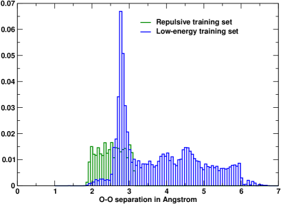
Figure 3: Distribution of O-O distances in the three-body training set, including all three O-O distances per trimer. “Low-energy” denotes configurations which were thermally accessible (see text for details).

It is important to mention that our initial model were fitted to a training set that emphasized only the low-energy and long-range regions, which is consistent with the parameterization strategy adopted for the WHBB 3B potentialWang et al. (2011). While the resulting models succeeded in predicting the relative stabilities of trimer and hexamer isomers, we found that they were numerically unstable in MD simulations of larger clusters, such as the 32-mer. This was related to insufficient coverage of the repulsive, short-ranged region of the trimer PES.

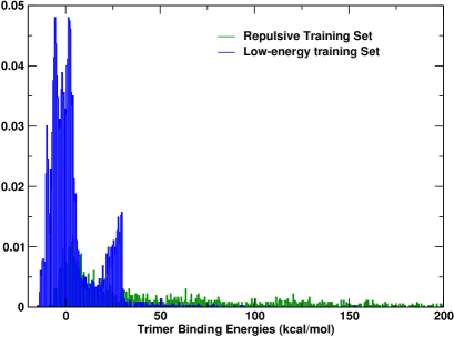
Figure 4: Distribution of trimer binding energies in the three-body training set.

To address this instability, 2072 configurations were generated by performing random rotations on monomers that were compressed relative to the trimer minimum geometry. As shown in Figure 3, this repulsive training set evenly covers O-O distances from 1.8 Å to 3.2 Å. Many of these compressed configurations, however, correspond to trimers that would practically never be sampled in simulations of water under ambient conditions. While including these configurations in the training set was required to ensure the numerical stability of the model, it was also necessary to guarantee that these highly-repulsive configurations did not degrade the quality of the fit in the region near the minimum. This consideration is discussed in the following section.

III.3 Testing the accuracy of the three-body fit

In order to assess the accuracy of any model with respect to ab initio data, it would be ideal to parameterize the model based on one set of reference data (the “training” set) and validate the model using a separate set of data (the “testing” set). However, due to the large computational cost associated with BSSE-corrected CCSD(T)/aug-cc-pVTZ 3B interactions and the fact that the model should be parametrized to as large of a reference set as possible, having two distinct sets is unfeasible. In order to estimate the bias associated with training and testing on the same reference data, the complete training set was equally divided into two parts, a training set and a testing set. Care was taken to preserve the relative compositions of each set, e.g., half of the 972 configurations extracted from simulations of ice were randomly selected and placed in the training set while the other half was placed in the testing set.

Since the goal of HBB2-pol is to describe water from small molecular clusters in the gas phase to condensed phases, we found it important to decompose the RMS into categories: 1) trimers with a binding energy of less than 5 kcal/mol, which are particularly important for low-temperature cluster isomer relative stabilities, 2) trimers with a binding energy of less than 30 kcal/mol, which are sampled during path-integral molecular dynamics (PIMD) simulations of bulk water at ambient conditions, and 3) the complete training set, regardless of binding energy (see Table 1). Due to the proximity of the energies for different isomers of the small clusters, it is desirable that 3B interactions corresponding to clusters with the lowest binding energies have the lowest RMS. As was discussed in Section III.2, it was necessary to include 3B energies corresponding to trimers with positive binding energies to ensure the stability of HBB2-pol. At the same time, care was taken to ensure that the accuracy in the low-energy region was not diluted by being needlessly accurate for trimers with enormous binding energies that will rarely be sampled. By appropriately weighting the reference data, HBB2-pol achieves the best accuracy in the low-energy region, slightly larger RMS in the intermediate region ($E_{bind}<5$ kcal/mol), and the largest error for those configurations with binding energies greater than 30 kcal/mol. To obtain this RMS distribution, configurations with 3B interactions were weighted according to their trimer binding energies, where configurations with $E_{bind}<15$ kcal/mol were given a weight of 1.0, while weights for configurations binding energies larger than 15 kcal/mol a weight of $e^{-a(E_{bind}-E_{0})}$, where a = 0.05 kcal/mol^-1 and $E_{0}$ was 15 kcal/mol.

Table 1: RMS deviation of three-body interactions from trimers with binding energies less than 5kcal/mol, less than 30kcal/mol, and for the complete training set. See main text for details.

	WHBB	$V_{ind}^{3B}$	HBB2-pol
	RMS for Training Set
Ebind $<$ 5	0.10	0.13	0.06
Ebind $<$ 30	0.14	0.35	0.10
Total	0.69	2.26	0.85
	RMS for Testing Set
Ebind $<$ 5	0.10	0.13	0.06
Ebind $<$ 30	0.15	0.35	0.16
Total	0.68	2.20	0.82
	RMS for Complete Set
Ebind $<$ 5	0.10	0.13	0.05
Ebind $<$ 30	0.14	0.34	0.11
Total	0.66	2.17	0.83

The results presented in Table 1 confirms the ability of the HBB2-pol 3B function to recover the ab initio data and demonstrates that the training set is sufficiently large to render the model insensitive to the size of the training set. This analysis does not, however, probe whether the training set includes all the physically relevant configurations. Assessing whether the composition of the training set is biased can only be accomplished by examining ab initio properties such as relative cluster isomer stabilities, experimental properties such as virial coefficients, and the overall numerical stability of the model.

III.4 HBB2-pol

Using the 3B interaction proposed in Eq. (2), HBB2-pol has been developed through the many-body expansion, Eq. (I). The spectroscopically-accurate monomer potential energy surface of Partridge and Schwenke is used for the 1B terms.Partridge and Schwenke (1997) For the 2B interaction, the HBB2 PESShank et al. (2009) is employed at short-range. The HBB2 short-range 2B interaction is smoothly switched to electrostatics/induction plus dispersion term at long-range over the interval $R^{2B}_{I}=5.5\text{\AA}<R_{\mathrm{OO}}<R^{2B}_{F}=7.5\text{\AA}$:

$$V^{2B} =(1-s_{2})V_{HBB2}^{2B}$$

$$+s_{2}\Big{[}V_{elec}^{2B}+V_{ind}^{2B}-\frac{C_{6}}{R_{\mathrm{OO}}^{6}}\Big{]},$$

$$s_{2} =\begin{cases}0&\xi\leq 0\\ \xi^{3}(10-15\xi+6\xi^{2})&0<\xi\leq 1\\ 1&1<\xi\end{cases},$$

where $\xi=(R_{\mathrm{OO}}-R_{I})\big{/}(R_{F}-R_{I})$. The $V_{elec}^{2B}$ and $V_{ind}^{2B}$ terms have the same form as TTM4-F, and the value of $C_{6}$ was taken as the difference between the sum of the ab initio van der Waals constants describing the dispersion and induction interactions in the asymptotic region from Ref. 49, and the $1/R_{\mathrm{OO}}^{6}$ coefficient of the isotropic part of $V_{ind}^{2B}$

$$C_{6}=(47.053232\;\mathrm{a.u.}+10.66517\;\mathrm{a.u})-2\alpha\mu^{2},$$

(using the isotropic molecular polarizability given by TTM4-F, $\alpha=1.41567$ Å³ the molecular dipole $\mu=1.864047$ D). The 3B interactions are those presented in Eq.(2), and all the higher-body terms are approximated by the induction energy as in TTM4-F,

$$V^{NB} =V_{ind}^{NB}-\sum_{i<j<k}^{N}V_{ind}^{3B}(i,j,k)$$

$$-\sum_{i<j}^{N}V_{ind}^{2B}(i,j).$$ (7)

Since $V_{HBB2}^{2B}$ accounts for polarization at the 2B level, the short-range 2B contribution must be subtracted from the N-body induction to prevent double counting. This problem does not arise for the 3B interactions since induction is not modified at the 3B level (Eq. (2)). The HBB2-pol interaction energy for $N$ water molecules is thus given by the following expression

$$E {}_{N-mer}=\sum_{i}^{N}V_{PS}^{1B}(i)$$

$$+\sum_{i<j}^{N}\biggl{\{}(1-s_{2})\bigl{[}V_{HBB2}^{2B}-V_{ind}^{2B}\bigr{]}+s_{2}\bigl{[}V_{elec}^{2B}-\frac{C_{6}}{R_{\mathrm{OO}}^{6}}\bigr{]}\biggr{\}}$$

$$+\sum_{i<j<k}^{N}s_{3}V_{poly}^{3B}(i,j,k)+V_{ind}^{NB}(1,\dots,N),$$ (8)

where the 3B switching functions, $s_{3}$, is given by Eq.(3).

IV Results

In this section we demonstrate the ability HBB2-pol to reproduce CCSD(T) calculations and the experimental second and third virial coefficients.

IV.1 Short-range Three-body Interaction Addresses Systematic Flaws in Polarizable Models

As discussed above, the three-body interactions primarily originate from induction, though for more strongly bound clusters effects including exhange-repulsion and charge transfer can also make a significant contribution.Mas et al. (2003); Chen and Gordon (1996) As a consequence, force fields which treat only induction are inherently unable to fully describe 3B interactions. By contrast, models that only treat short-range 3B interactions are unable to describe the induction interactions that dominate at long range. This is illustrated in Figure 5, where HBB2-pol is compared with WHBB, TTM4-F 3B induction, and CCSD(T)/aug-cc-pVTZ data along two representative cuts through the water trimer PES. The CCSD(T) reference data used for this comparison were not included in the training set. This comparison clearly shows that the addition of the short-range “correction” to the induction brings the 3B interactions of HBB2-pol into close agreement with the CCSD(T) data.

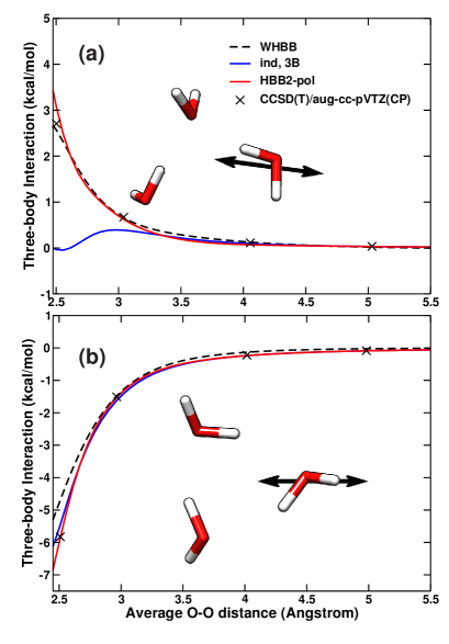
Figure 5: Three-body interaction energy for two cuts through the water trimer potential energy surface: WHBB (black dashes), three-body induction (blue), HBB2-pol (red) and CCSD(T)/aug-cc-pVTZ (crosses).

IV.2 Trimer stationary points

To assess the combined accuracy of the 1B, 2B, and 3B interactions of HBB2-pol, we studied the relative energies of four water trimer isomers identified in Table 2 by their free-hydrogen orientation: “u” for pointing up, “p” if the hydrogen lies in the plane of the oxygen atoms, and “d” for pointing down. The energetics of these structures have been reported in Ref. 75, where geometries optimized at the MP2/aug-cc-pVQZ level were used to calculate the energies at the CCSD(T) level in the complete basis limit. The HBB2-pol energies relative to the trimer global minimum (uud) are reported in Table 2 for the geometries optimized on the HBB2-pol PES. These favorably interacting trimers have CCSD(T) binding energies of approximately -15 kcal/mol, which implies that the energies separating these stationary points are on the order of 1-10% of the binding energy. The HBB2-pol relative energies fall within 0.05 kcal/mol of the reference data for the upd and uuu structures, while a larger difference of 0.23 kcal/mol is obtained for the ppp structure. HBB2-pol, however, is not expected to achieve perfect agreement with the CCSD(T)/CBS dataAnderson et al. (2004) due to the different basis set used in the fit of the 3B terms.

Table 2: Relative energies of water trimer isomers with respect to the global minimum “uud” in kcal/mol. CCSD(T) energies were extrapolated to complete basis set limit, from Ref. 75.

	CCSD(T)	HBB2-pol
uud	0.0	0.0
upd	0.23	0.18
uuu	0.77	0.73
ppp	1.25	1.02

IV.3 Virial coefficients

Virial coefficients are derived from the virial equation of state that expresses $p/k_{B}T$ as a power series in density and gauge deviations from the ideal gas behavior,

$$\frac{p}{k_{B}T}=\frac{N}{V}\biggl{[}1+B_{2}\frac{N}{V}+B_{3}\biggl{(}\frac{N}{V}\biggr{)}^{2}+...\biggr{]}.$$ (9)

Here, $B_{2}$ and $B_{3}$ are the second and third virial coefficients, respectively.Hill (1986); Mayer and Mayer (1940); Mason and Spurling (1969) The second virial coefficient depends only on the pair interaction while the third virial coefficient also includes the 3B interaction, but no $(n>3)$-body energies. Since both $B_{2}$ and $B_{3}$ are experimentally accessible, the virial coefficients provide a critical assessment of the accuracy of water potentials.

Neglecting the contribution of intramolecular vibrational modes (that is, assuming rigid monomers) and nuclear quantum effects, the second virial coefficient is given byMason and Spurling (1969),

$$B_{2}(T) =-2\pi\int\mathrm{d}R_{12}\,R_{12}^{2}\bigl{<}f_{12}\bigr{>}_{\bm{\Omega}_{1},\bm{\Omega}_{2}},$$

$$f_{12} =\mathrm{e}^{-\beta V^{2B}(R_{12},\bm{\Omega_{1}},\bm{\Omega_{2})}}-1,$$ (10)

where $\beta=1/k_{B}T$ is the inverse temperature, $R_{12}$ is the distance between the monomer centers of mass, $V^{2B}(R_{12},\bm{\Omega_{1}},\bm{\Omega_{2}})$ is the intermolecular interaction energy, and the angular brackets stand for the average over the orientations of the molecules $\bm{\Omega}_{1,2}$. The Mayer function, $f_{12}$, has the useful property of going to zero as the molecules move apart. To numerically evaluate Eq. (IV.3), the Simpson rule is used to calculate the radial component of the integral, while Monte Carlo integration is used to evaluate the orientational average using $10^{5}$ random orientations of the monomers at each point on the radial grid.

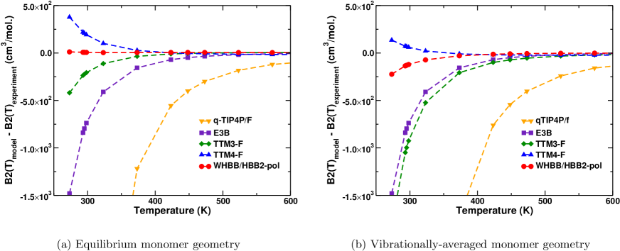
Figure 6: Effect of the rigid monomer configuration on the error in the classical second virial coefficient relative to experiment.Harvey and Lemmon (2004) Differences between WHBB and HBB2-pol were indistinguishable on the scale of this plot, so both have been assigned to the red line. For E3B, its rigid monomer geometry was used in both plots.

To explore the sensitivity of the second virial coefficient to the choice of the rigid monomer geometry, its values are calculated using two different configurations: the Born-Oppenheimer minimum energy configuration given by the Partridge-Schwenke potential energy surface ($r_{OH}^{eq}=0.95784\text{\AA}$ and $\theta_{HOH}^{eq}=104.508^{\circ}$) Partridge and Schwenke (1997), and the ground-state vibrationally-averaged configuration of $r_{OH}^{eq}=0.9716256\text{\AA}$ and reported in reference 80 ($\theta_{HOH}^{eq}=104.69^{\circ}$). Importantly, examining the results for these two configurations provides not only an estimate of the effect of flexibility, but also of nuclear quantum effects “sensed” through the ground-state vibrationally averaged configuration.

Plotted in Figure 6 is the difference between the calculated virial coefficients and the experimental data.Harvey and Lemmon (2004) Since $B_{2}$ is the integral of $e^{-\beta V^{2B}}-1$, comparison to low-temperature results are particularly interesting as these are most sensitive to the region near the dimer minimum geometry. For the Born-Oppenheimer equilibrium geometries (Fig. 6a), the ab initio-based potential energy surfaces WHBB and HBB2-pol very closely reproduce the experimental data. Since HBB2-pol and WHBB share the same two-body PES at dimer separations of less than 5.5Å, it is not surprising that both models predict similar values for the second virial coefficient. Though detectable, the differences between WHBB and HBB2-pol are not visible on the scale of Figure 6, so both have been assigned to the red line.

While both qTIP4P/f and E3B were empirically parametrized, the inclusion of explicit 3B interactions in E3B allows for a more accurate 2B interaction. Pairwise-additive models, such as qTIP4P/f, on the other hand, rely on the 2B interaction to (partially) recover 3B effects and would therefore be expected to have a much larger error for the second virial coefficient. When the monomer geometry is changed from the equilibrium to the vibrationally-averaged geometry, there is a small decrease in the value of $B_{2}(T)$ for most models. TTM3-F, however, exhibits a large change in its second virial coefficient. This is likely due to the empirical modification of the dipole moment surface, which only affects TTM3-F when the monomer distorts from the equilibrium configuration.Fanourgakis and Xantheas (2008)

The third virial coefficient depends on the interaction of trimers and provides an indirect measure of the 3B interaction. Following HillHill (1986), the third virial coefficient can be separated into a pairwise component, $B_{3}^{0}(T)$, and the 3B contribution, $\Delta B_{3}^{3B}(T)$:

$$B_{3}(T)=B_{3}^{0}(T)+\Delta B_{3}^{3B}(T),$$ (11)

where the pairwise contribution is the integral over the product of the three Mayer functions in Eq. (12), and the 3B contribution is given by Eq. (13).

$$B_{3}^{0}(T)=-\frac{8}{3}\pi^{2}\int\mathrm{d}R_{12}\mathrm{d}R_{13}\,R_{12}^{2}R_{13}^{2}\bigl{<}f_{12}f_{13}f_{23}\sin\vartheta_{(2,1,3)}\bigr{>}_{\bm{\Omega}_{1},\bm{\Omega}_{2},\bm{\Omega}_{3},\vartheta_{(2,1,3)}},$$ (12)

$$\Delta B_{3}^{3B}(T)=-\frac{8}{3}\pi^{2}\int\mathrm{d}R_{12}\mathrm{d}R_{13}\,R_{12}^{2}R_{13}^{2}\biggl{<}\bigl{[}\mathrm{e}^{-\beta V_{1,2,3}^{3B}}-1\bigr{]}\mathrm{e}^{-\beta(V_{1,2}^{2B}+V_{1,3}^{2B}+V_{2,3}^{2B})}\sin\vartheta_{(2,1,3)}\biggr{>}_{\bm{\Omega_{1}},\bm{\Omega_{2}},\bm{\Omega_{3}},\vartheta_{(2,1,3)}}.$$ (13)

Following the work of Tainter et al.,Tainter et al. (2011) we computed the third virial coefficient by fixing one molecule at the origin, evaluating two radial integrals through the two-dimensional Simpson rule, and using Monte Carlo integration for the 9 orientational degrees of freedom and the angle $\vartheta_{(2,1,3)}$ between the centers of mass of molecules 2, 1, 3 at each radial grid point (using $10^{6}$ monomer orientations). This integration strategy was demonstrated in Ref. 24 to recover the results from the more efficient Mayer sampling approach.Benjamin et al. (2007) Our implementation reproduces the data from Ref. 24 for the E3B model.

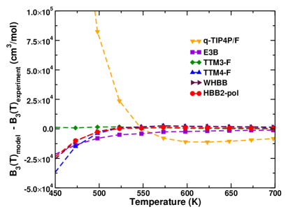
Figure 7: Rigid, classical third virial coefficient using vibrationally-averaged monomer geometries. Experimental data from Ref. 82.

Rigid, classical third virial coefficients using vibrationally-averaged monomer geometries are reported in figure 7. At lower temperatures, HBB2-pol agrees with WHBB. In the high temperature limit, however, HBB2-pol compare more favorably with experiment than WHBB, which is consistent with HBB2-pol providing a more accurate description of the 3B interactions. The errors in the 2B and 3B interactions of TTM3-F appear to cancel one another, resulting in an third virial coefficient that is remarkably close to experiment. Much work has been invested in exploring the role of nuclear quantum effects Garberoglio (2012); Schenter (2002); Bukowski et al. (2008) and monomer flexibility.Shaul et al. (2011) While the exploration of the monomer configuration on the second virial coefficient indicates that flexibility and nuclear quantum effects are important, these results are by no means conclusive. We will pursue a more rigorous characterization of the effect of flexibility and nuclear quantization in future work.

V Summary

In this study, the accuracy of several force fields, semiempirical methods, DFT, and ab initio-based models in reproducing the two- and three-body water interactions was assessed against BSSE-corrected CCSD(T)/aug-cc-pVTZ data. Our analysis of the many-body expansion of the interaction energy indicates that defects inherent to polarizable models, which are non-negligable when molecules are close to one another, can be effectively corrected through an explicit short-range term expressed in terms of permutationally invariant polynomials. Based on these findings, we developed a new water model, HBB2-pol, that is derived entirely from “first principles”. HBB2-pol achieves excellent accuracy with respect to the CCSD(T) data for the two- and three-body interactions, isomer relative energies of small clusters, and second and third virial coefficients. Importantly, the inclusion of explicit polarization in the three-body interaction term enables the use of relatively low-degree polynomials, which, in turn, results in a significant decrease in the computational cost associated with HBB2-pol relative to other ab initio-based models. Through its combined accuracy and computational efficiency, HBB2-pol thus opens the doorway to fully “first principles” simulations of water in the condensed phases, which will help resolve current controversiesWernet et al. (2004); Clark et al. (2010); Pieniazek et al. (2011); Nihonyanagi et al. (2011); Kumar et al. (2008); Limmer and Chandler (2011).

VI Acknowledgement

This research was supported by the National Science Foundation through grant CHE-1111364. We are grateful to the National Science Foundation for a generous allocation of computing time on Xsede resources (award TG-CHE110009). Additionally, we would like to thank Chris Mundy and Greg Schenter for their assistance in calculations involving SCP-NDDO.

References

- Dahlke et al. (2008) Dahlke, E.; Olson, R.; Leverentz, H.; Truhlar, D. J. Phys. Chem. A 2008, 112, 3976–84.
- Bates and Tschumper (2009) Bates, D.; Tschumper, G. J. Phys. Chem. A 2009, 113, 3555–3559.
- Góra et al. (2011) Góra, U.; Podeszwa, R.; Cencek, W.; Szalewicz, K. J. Chem. Phys. 2011, 135, 224102.
- Soper and Benmore (2008) Soper, A.; Benmore, C. Phys. Rev. Lett. 2008, 101, 065502.
- Paesani and Voth (2009) Paesani, F.; Voth, G. J. Phys. Chem. B 2009, 113, 5702–19.
- Wang et al. (2012) Wang, Y.; Babin, V.; Bowman, J.; Paesani, F. J. Am. Chem. Soc. 2012, 134, 11116–9.
- Markland and Berne (2012) Markland, T.; Berne, B. Proc. Natl. Acad. Sci. 2012, 109, 7988–7991.
- Hankins et al. (1970) Hankins, D.; Moskowitz, J.; Stillinger, F. J. Chem. Phys. 1970, 53, 4544–4554.
- Xantheas (1994) Xantheas, S. J. Chem. Phys. 1994, 100, 7523–7534.
- Xantheas (2000) Xantheas, S. Chem. Phys. 2000, 258, 225–231.
- Defusco et al. (2007) Defusco, A.; Schofield, D.; Jordan, K. Mol. Phys. 2007, 105, 2681–2696.
- Kumar et al. (2010) Kumar, R.; Wang, F.; Jenness, G.; Jordan, K. J. Chem. Phys. 2010, 132, 014309.
- Hodges et al. (1997) Hodges, M.; Stone, A.; Xantheas, S. J. Phys. Chem. A 1997, 101, 9163–9168.
- Ojamie and Hermansson (1994) Ojamie, L.; Hermansson, K. J. Phys. Chem. 1994, 98, 4271–4282.
- Pedulla et al. (1996) Pedulla, J.; Vila, F.; Jordan, K. J. Chem. Phys. 1996, 105, 11091.
- Cui et al. (2006) Cui, J.; Liu, H.; Jordan, K. J. Phys. Chem. B 2006, 110, 18872–18878.
- Hermann et al. (2007) Hermann, A.; Krawczyk, R.; Lein, M.; Schwerdtfeger, P.; Hamilton, I.; Stewart, J. Phys. Rev. A 2007, 76, 013202.
- Jorgensen et al. (1983) Jorgensen, W.; Chandrasekhar, J.; Madura, J.; Impey, R.; Klein, M. J. Chem. Phys. 1983, 79, 926.
- Berendsen et al. (1981) Berendsen, H.; Postma, J.; van Gunsteren, W.; Hermans, J. In Intermolecular Forces; Pullman, B., Ed.; Reidel Publishing Company: Dordrecht, 1981; pp 333–342.
- Habershon et al. (2009) Habershon, S.; Markland, T.; Manolopoulos, D. J. Chem. Phys. 2009, 131, 024501.
- Paesani et al. (2006) Paesani, F.; Zhang, W.; Case, D.; Cheatham, T.; Voth, G. J. Chem. Phys. 2006, 125, 184507.
- Vega and Abascal (2011) Vega, C.; Abascal, J. Phys. Chem. Chem. Phys. 2011, 13, 19663–19688.
- Kumar and Skinner (2008) Kumar, R.; Skinner, J. J. Phys. Chem. B 2008, 112, 8311–8318.
- Tainter et al. (2011) Tainter, C.; Pieniazek, P.; Lin, Y.; Skinner, J. J. Chem. Phys. 2011, 134, 184501.
- Tainter and Skinner (2012) Tainter, C.; Skinner, J. J. Chem. Phys. 2012, 137, 104304.
- Lopes et al. (2009) Lopes, P.; Roux, B.; Mackerell, A. Theor. Chem. Acc. 2009, 124, 11–28.
- Applequist et al. (1972) Applequist, J.; Carl, J.; Fung, K. J. Am. Chem. Soc. 1972, 94, 2952–2960.
- Thole (1981) Thole, B. Chem. Phys. 1981, 59, 341–350.
- Fanourgakis and Xantheas (2008) Fanourgakis, G.; Xantheas, S. J. Chem. Phys. 2008, 128, 074506.
- Burnham et al. (2008) Burnham, C.; Anick, D.; Mankoo, P.; Reiter, G. J. Chem. Phys. 2008, 128, 154519.
- Ren and Ponder (2003) Ren, P.; Ponder, J. J. Phys. Chem. B 2003, 107, 5933–5947.
- Stewart (1989) Stewart, J. J. Comput. Chem. 1989, 10, 209–220.
- Bernal-Uruchurtu and Ruiz-López (2000) Bernal-Uruchurtu, M.; Ruiz-López, M. Chem. Phys. Lett. 2000, 330, 118–124.
- Chang et al. (2008) Chang, D.; Schenter, G.; Garrett, B. J. Chem. Phys. 2008, 128, 164111.
- Murdachaew et al. (2011) Murdachaew, G.; Mundy, C.; Schenter, G.; Laino, T.; Hutter, J. J. Phys. Chem. A 2011, 115, 6046–53.
- Becke (1988) Becke, A. Phys. Rev. A 1988, 38, 3098–3100.
- Lee et al. (1988) Lee, C.; Yang, W.; Parr, R. Phys. Rev. B 1988, 37, 785–789.
- Perdew et al. (1996) Perdew, J.; Burke, K.; Ernzerhof, M. Phys. Rev. Lett. 1996, 77, 3865–3868.
- Grimme (2004) Grimme, S. J. Comput. Chem. 2004, 25, 1463–1473.
- Grimme (2006) Grimme, S. J. Comput. Chem. 2006, 27, 1787–1799.
- Fulton et al. (2010) Fulton, J.; Schenter, G.; Baer, M.; Mundy, C.; Dang, L.; Balasubramanian, M. J. Phys. Chem. B 2010, 114, 12926–12937.
- Ma et al. (2012) Ma, Z.; Zhang, Y.; Tuckerman, M. J. Chem. Phys. 2012, 044506, 044506.
- Grimme et al. (2010) Grimme, S.; Antony, J.; Ehrlich, S.; Krieg, H. J. Chem. Phys. 2010, 132, 154104.
- Dion et al. (2004) Dion, M.; Rydberg, H.; Schröder, E.; Langreth, D.; Lundqvist, B. Phys. Rev. Lett 2004, 92, 246401.
- Lee et al. (2010) Lee, K.; Murray, E.; Kong, L.; Lundqvist, B.; Langreth, D. Phys. Rev. B 2010, 82, 081101.
- Vydrov and Van Voorhis (2010) Vydrov, O.; Van Voorhis, T. J. Chem. Phys. 2010, 133, 244103.
- Wang et al. (2011) Wang, J.; Román-Pérez, G.; Soler, J.; Artacho, E.; Fernández-Serra, M. J. Chem. Phys. 2011, 134, 024516.
- Murray and Galli (2012) Murray, E.; Galli, G. Phys. Rev. Lett. 2012, 108, 105502.
- Bukowski et al. (2008) Bukowski, R.; Szalewicz, K.; Groenenboom, G.; van Der Avoird, A. J. Chem. Phys. 2008, 128, 094314.
- Bukowski et al. (2008) Bukowski, R.; Szalewicz, K.; Groenenboom, G.; van Der Avoird, A. J. Chem. Phys. 2008, 128, 094313.
- Wang et al. (2011) Wang, Y.; Huang, X.; Shepler, B.; Braams, B.; Bowman, J. J. Chem. Phys. 2011, 134, 094509.
- Bukowski et al. (2007) Bukowski, R.; Szalewicz, K.; Groenenboom, G.; van der Avoird, A. Science 2007, 315, 1249–52.
- Leforestier et al. (2012) Leforestier, C.; Szalewicz, K.; van der Avoird, A. J. Chem. Phys. 2012, 137, 014305.
- Raghavachari et al. (1989) Raghavachari, K.; Truck, G.; Pople, J.; Head-Gordon, M. Chem. Phys. Lett. 1989, 157, 479–483.
- Dunning (1989) Dunning, T. J. Chem. Phys. 1989, 90, 1007.
- Boys and Bernardi (1970) Boys, S.; Bernardi, F. Mol. Phys. 1970, 19, 553.
- Weigend and Ahlrichs (2005) Weigend, F.; Ahlrichs, R. Phys. Chem. Chem. Phys. 2005, 7, 3297–3305.
- Schafer et al. (1994) Schafer, A.; Huber, C.; Ahlrichs, R. J. Chem. Phys. 1994, 100, 5829–5835.
- Wennmohs and Neese (2008) Wennmohs, F.; Neese, F. Chem. Phys. 2008, 343, 217–230.
- Walker et al. (2008) Walker, R. C.; Crowley, M. F.; Case, D. A. J. Comput. Chem. 2008, 29, 1019–1031.
- cp (2) http://cp2k.berlios.de/ 2000–2012.
- Murdachaew et al. (2011) Murdachaew, G.; Mundy, C.; Schenter, G.; Laino, T.; Hutter, J. J. Phys. Chem. A 2011, 115, 6046–6053.
- Burnham and Xantheas (2002) Burnham, C.; Xantheas, S. J. Chem. Phys. 2002, 116, 5115.
- VandeVondele and Hutter (2007) VandeVondele, J.; Hutter, J. J. Chem. Phys. 2007, 127, 114105.
- Becke (1993) Becke, A. J. Chem. Phys 1993, 98, 5648.
- Stephens et al. (1994) Stephens, P.; Devlin, F.; Chabalowski, C.; Frisch, M. J. Phys. Chem. 1994, 98, 11623–11627.
- Klimes and Michaelides (2012) Klimes, J.; Michaelides, A. J. Chem. Phys. 2012, 137, 120901.
- Chen and Gordon (1996) Chen, W.; Gordon, M. J. Phys. Chem. 1996, 100, 14316–14328.
- Shank et al. (2009) Shank, A.; Wang, Y.; Kaledin, A.; Braams, B.; Bowman, J. J. Chem. Phys. 2009, 130, 144314.
- Mas et al. (2003) Mas, E.; Bukowski, R.; Szalewicz, K. J. Chem. Phys. 2003, 118, 4386–4403.
- Caldwell et al. (1990) Caldwell, J.; Dang, L.; Kollman, P. J. Am. Chem. Soc 1990, 112, 9144–9147.
- Galassi (2009) Galassi, M. GNU Scientific Library Reference Manual, 3rd ed.; Network Theory Ltd., 2009.
- (73) Maple 11, Maplesoft, a division of Waterloo Maple Inc., Waterloo, Ontario
- Partridge and Schwenke (1997) Partridge, H.; Schwenke, D. J. Chem. Phys. 1997, 106, 4618.
- Anderson et al. (2004) Anderson, J.; Crager, K.; Fedoroff, L.; Tschumper, G. J. Chem. Phys. 2004, 121, 11023–11029.
- Hill (1986) Hill, T. An Introduction to Statistical Thermodynamics; Dover, 1986.
- Mayer and Mayer (1940) Mayer, J.; Mayer, M. Statistical Mechanics; John Wiley & Sons Inc, 1940.
- Mason and Spurling (1969) Mason, E.; Spurling, T. International encyclopedia of physical chemistry and chemical physics. Topic 10, Fluid state, V. 2; Pergamon Press: New York, 1969.
- Harvey and Lemmon (2004) Harvey, A.; Lemmon, E. J. Phys. Chem. Ref. Data. 2004, 33, 369–376.
- Mas and Szalewicz (1996) Mas, E.; Szalewicz, K. J. Chem. Phys. 1996, 104, 7606.
- Benjamin et al. (2007) Benjamin, K.; Singh, J.; Schultz, A.; Kofke, D. J. Phys. Chem. B 2007, 111, 11463–11473.
- Kell et al. (1989) Kell, G.; McLaurin, G.; Whalley, E. Proc. R. Soc. Lond. A 1989, 425, 49–71.
- Garberoglio (2012) Garberoglio, G. Chem. Phys. Lett. 2012, 525-526, 19–23.
- Schenter (2002) Schenter, G. J. Chem. Phys. 2002, 117, 6573.
- Shaul et al. (2011) Shaul, K.; Schultz, A.; Kofke, D. J. Chem. Phys. 2011, 135, 124101.
- Wernet et al. (2004) Wernet, P.; Nordlund, D.; Bergmann, U.; Cavalleri, M.; Odelius, M.; Ogasawara, H.; Näslund, L.; Hirsch, T.; Ojamäe, L.; Glatzel, P.; Pettersson, L.; Nilsson, A. Science 2004, 304, 995–999.
- Clark et al. (2010) Clark, G.; Cappa, C.; Smith, J.; Saykally, R.; Head-Gordon, T. Mol. Phys. 2010, 108, 1415–1433.
- Pieniazek et al. (2011) Pieniazek, P.; Tainter, C.; Skinner, J. J. Am. Chem. Soc. 2011, 133, 10360.
- Nihonyanagi et al. (2011) Nihonyanagi, S.; Ishiyama, T.; Lee, T.; Yamaguchi, S.; Bonn, M.; Morita, A.; Tahara, T. J. Am. Chem. Soc. 2011, 133, 16875–16880.
- Kumar et al. (2008) Kumar, P.; Franzese, G.; Eugene Stanley, H. J. Phys. Condens. Matter 2008, 20, 244114.
- Limmer and Chandler (2011) Limmer, D.; Chandler, D. J. Chem. Phys. 2011, 135, 134503.