Optimization of QCD Perturbation Theory:

Results for $R_{e^{+}e^{-}}$ at fourth order

P. M. Stevenson

T.W. Bonner Laboratory, Department of Physics and Astronomy,
Rice University, Houston, TX 77251, USA

Abstract:

Physical quantities in QCD are independent of renormalization scheme (RS), but that exact invariance is spoiled by truncations of the perturbation series. “Optimization” corresponds to making the perturbative approximant, at any given order, locally invariant under small RS changes. A solution of the resulting optimization equations is presented. It allows an efficient algorithm for finding the optimized result. Example results for $R_{e^{+}e^{-}}=3\sum q_{i}^{2}(1+{\cal R})$ to fourth order (NNNLO) are given that show nice convergence, even down to arbitrarily low energies. The $Q=0$ “freezing” behaviour, ${\cal R}=0.3\pm 0.3$, found at third order is confirmed and made more precise; ${\cal R}=0.2\pm 0.1$. Low-energy results in the $\overline{\rm MS}$ scheme, by contrast, show the typical pathologies of a non-convergent asymptotic series.

1 Introduction

Renormalization, for physical quantities in massless QCD, amounts to eliminating the bare coupling constant in favour of a renormalized couplant. The precise definition of the renormalized couplant — the renormalization scheme (RS) — is in principle arbitrary, but at finite orders of perturbation theory the choice matters. It is well known that one can take advantage of this situation by allowing the renormalization scale, $\mu$, to “run” with the experimental energy scale $Q$, but this familiar idea is vague and incomplete. What matters is not $\mu$, in fact, but the ratio of $\mu$ to $\Lambda$, itself a RS-dependent parameter — and, at higher orders, there are further sources of RS ambiguity. “Optimized perturbation theory” (OPT) [1] provides both a complete parametrization of RS dependence and the means to sensibly resolve these ambiguities by taking full advantage of Renormalization-Group (RG) invariance [2].

The aim of this paper is twofold: (i) to present a mathematical solution to the “optimization equations” of Ref. [1], allowing the optimized result to be found efficiently; and (ii) to show numerical results for $R_{e^{+}e^{-}}\equiv\sigma(e^{+}e^{-}\to{\mbox{\rm hadrons}})/\sigma(e^{+}e^{-}\to\mu^{+}\mu^{-})$, updating the results of Refs. [3, 4, 5] now that fourth-order calculations are available [6].

The RS-dependence problem remains a controversial topic. Our arguments have been set out in detail in Refs. [1] and [7]–[10]. Here we give only a brief exposition of the key idea behind OPT, the “principle of minimal sensitivity.” This is the very general notion that, in any approximation method involving “extraneous” parameters (parameters that one knows the exact result must be independent of), the sensible strategy is to find where the approximant is minimally sensitive to small variations of those parameters. The unknown exact result is globally invariant, while the approximant is not; where the approximant has the right qualitative behaviour — local invariance (flatness as a function of the extraneous parameters) — is where one can have most confidence in its quantitative value. Many instructive examples testify to the basic soundness and power of this idea (see [1],[11]–[15]).

In the present context, RG invariance tells us that physical quantities should be independent of $\mu$ and all the other “extraneous” parameters involved in the RS choice. That statement translates into an infinite set of equations (Eqs. (2.1) below) that any physical quantity ${\cal R}$ must satisfy [1]. Perturbative approximations to ${\cal R}$ do not satisfy these equations, but we can find an “optimal RS” in which they are satisfied locally. We explain in this paper how these optimization equations can be solved efficiently.

Calculations in QCD perturbation theory, in particular for $\beta$ and $R_{e^{+}e^{-}}$, have progressed from leading order (LO) [16], to next-to-leading order (NLO) [17, 18], to next-to-next-to-leading (NNLO or N²LO) [19, 20], to now next-to-next-to-next-to-leading order (NNNLO or N³LO) [21, 6]. (We will use the terminology “first order” for leading order (LO) and “$(k+1)^{th}$ order” for N^kLO.) Tribute should be paid at this point to the heroic efforts involved in these enormously complex calculations. The results allow us now to get a real sense of how QCD perturbation theory behaves, both in a fixed RS and with the optimization procedure.

Perturbation series, in any fixed RS, are expected to be factorially divergent. However, it is possible that the optimized results converge, thanks to an “induced convergence” mechanism in which the optimized couplant shrinks from one order to the next [22] (see also [23, 12, 15]). Our numerical results here are quite consistent with that idea.

The plan of this paper is as follows: Section 2 reviews the mathematical consequences of RG invariance derived in Ref. [1]. Section 3 discusses finite-order approximants and explains how to “optimize” the RS choice based on the principle of minimal sensitivity. Section 4 solves the resulting optimization equations, in a general $(k+1)^{th}$ order, and Section 5 outlines an algorithm to determine the result efficiently. Section 6 applies this algorithm to obtain illustrative results for $R_{e^{+}e^{-}}$ in second, third, and fourth orders and compares them with results in a fixed scheme, $\overline{\rm MS}(\mu=Q)$. The optimized results exhibit steady convergence — even down to zero energy, where the limit ${\cal R}=0.3\pm 0.3$, found in third order [3, 4, 5], is confirmed and made more precise; ${\cal R}=0.2\pm 0.1$. The fixed-scheme results show pathologies at low energies and we argue that these are a preview of what one can expect at higher orders at higher energies. Concluding remarks are in Section 7. Appendix A proves an identity mentioned in Section 4, and Appendix B discusses optimization in the fixed-point ($Q\to 0$) limit, following Ref. [24].

2 RG invariance and its consequences

2.1 RG equations

We begin by reviewing the formalism introduced in Ref. [1]. First, we emphasize that OPT can only be applied to physical quantities (cross sections, decay rates, etc.). QCD involves many other objects – Green’s functions, renormalized couplants, etc. – that are not physically measurable and are not RS invariant; for our purposes these are merely intermediate steps in calculating physical quantities and need not be discussed. In general, a perturbatively calculable physical quantity will have the form $A_{1}{\cal R}+A_{0}$ with a leading-order coefficient $A_{1}$ and, sometimes, a zeroth-order term $A_{0}$. The coefficients $A_{0}$ and $A_{1}$, which carry dimensions of energy to the appropriate power, are RS invariant, so we may focus on dimensionless, normalized physical quantities ${\cal R}$ of the form:

$${\cal R}=a^{{\scriptstyle{{\rm P}}}}(1+r_{1}a+r_{2}a^{2}+\ldots),$$ (2.1)

where $a\equiv\alpha_{s}/\pi$ is the renormalized couplant. The power ${\scriptstyle{{\rm P}}}$ is usually $1$ or $2$ or $3$, but need not be an integer. Generally a physical quantity ${\cal R}$ is not a single quantity but rather a function of several experimentally defined parameters. We may always single out one such parameter with the dimensions of energy that we may call the “experimental energy scale” and denote by “$Q$.” (It is needed only to explain which quantities are, or are not, $Q$ dependent; the precise definition of $Q$ in any specific case is left to the reader.) Note that $Q$ must be defined in experimental terms and should not be confused with the renormalization scale $\mu$, which is defined only in terms of the technical details of the RS adopted.

In the specific case of $R_{e^{+}e^{-}}$ where, ignoring quark masses,

$$R_{e^{+}e^{-}}=3\sum q_{i}^{2}(1+{\cal R}),$$ (2.2)

we have ${\scriptstyle{{\rm P}}}=1$ and the $e^{+}e^{-}$ center-of-mass energy is a natural choice for $Q$.

The fundamental notion of RG invariance [2] means that a physical quantity is independent of the renormalization scheme (RS). Expressed symbolically it states that

$$0=\frac{d{\cal R}}{d(RS)}=\left.\frac{\partial{\cal R}}{\partial(RS)}\right|_{a}+\frac{da}{d(RS)}\frac{\partial{\cal R}}{\partial a},$$ (2.3)

where the total derivative is separated into two pieces corresponding, respectively, to RS dependence from the $r_{i}$ series coefficients, and from the couplant $a$ itself. A particular case of Eq. (2.3) is the familiar equation expressing the renormalization-scale independence of ${\cal R}$:

$$\left(\left.\mu\frac{\partial}{\partial\mu}\right|_{a}+\beta(a)\frac{\partial}{\partial a}\right){\cal R}=0,$$ (2.4)

where

$$\beta(a)\equiv\mu\frac{da}{d\mu}=-ba^{2}(1+ca+c_{2}a^{2}+c_{3}a^{3}+\ldots).$$ (2.5)

The first two coefficients of the $\beta$ function are RS invariant [25] and, in QCD with $n_{f}$ massless flavours, are given by [16, 17]:

$$b=\frac{(33-2n_{f})}{6},\quad\quad c=\frac{153-19n_{f}}{2(33-2n_{f})}.$$ (2.6)

When integrated, the $\beta$-function equation can be written as:

$$\int_{0}^{a}\frac{da^{\prime}}{\beta(a^{\prime})}+{\cal C}=\int_{\tilde{\Lambda}}^{\mu}\frac{d\mu^{\prime}}{\mu^{\prime}}=\ln(\mu/{\tilde{\Lambda}}).$$ (2.7)

where ${\cal C}$ is a suitably infinite constant and $\tilde{\Lambda}$ is a constant with dimensions of mass. The particular definition of $\tilde{\Lambda}$ that we use corresponds to choosing [1]

$${\cal C}=\int_{0}^{\infty}\frac{da^{\prime}}{b{a^{\prime}}^{2}(1+ca^{\prime})}$$ (2.8)

(where it is to be understood that the integrands on the left of (2.7) are to be combined before the bottom limit is taken). This $\tilde{\Lambda}$ parameter is related to the traditional definition [26, 27] by an RS-invariant, but $n_{f}$-dependent factor [1, 28]:

$$\ln(\Lambda/\tilde{\Lambda})=(c/b)\ln(2c/b).$$ (2.9)

The $\tilde{\Lambda}$ parameter is scheme dependent, but the $\tilde{\Lambda}$-parameters of two schemes are related by the Celmaster-Gonsalves relation [29]. If two schemes are related, for the same value of $\mu$, by

$$a^{\prime}=a(1+v_{1}a+\ldots)$$ (2.10)

then

$$\ln(\tilde{\Lambda}^{\prime}/\tilde{\Lambda})=v_{1}/b.$$ (2.11)

This relationship is exact and does not involve the $v_{2},v_{3},\ldots$ coefficients. Thus, the $\tilde{\Lambda}$’s of different schemes can be related exactly by a 1-loop calculation. Hence, the $\tilde{\Lambda}$ parameter of any convenient “reference RS” can be adopted, without prejudice, as the one free parameter of the theory, taking over the role of the “bare coupling constant” in the original Lagrangian.

From Eq. (2.7) it is clear that $a$ depends on RS only through the variables $\mu/\tilde{\Lambda}$ and $c_{2},c_{3},\ldots$, the scheme-dependent $\beta$-function coefficients. The coefficients of ${\cal R}$ can depend on RS only through these same variables — the RG-invariance equation, (2.3), could not be satisfied otherwise. Therefore, these variables provide a complete RS parametrization, as far as physical quantities are concerned [1]. Thus, we may write:

$$a=a({\rm RS})=a(\tau,c_{2},c_{3},\ldots),$$ (2.12)

where

$$\tau\equiv b\ln(\mu/\tilde{\Lambda}).$$ (2.13)

The $\tau$ variable is convenient and helps to emphasize the important point that $\mu$ itself is not meaningful because of the scheme ambiguity represented by Eq. (2.10); only the ratio of $\mu$ to $\tilde{\Lambda}$ matters.

The dependence of $a$ on the set of RS parameters $\tau$ and $c_{j}$ is given by [1]:

$$\frac{\partial a}{\partial\tau}=\beta(a)/b,$$ (2.14)

$$\frac{\partial a}{\partial c_{j}}\equiv\beta_{j}(a)=-b\beta(a)\int_{0}^{a}dx\;\frac{x^{j+2}}{\beta(x)^{2}},$$ (2.15)

where the first equation is just the $\beta$-function equation in new notation, and the second follows by taking the partial derivative of Eq. (2.7) with respect to $c_{j}$, holding $\tau$ and the other $c_{i}$ ($i\neq j$) constant.

The symbolic RG-invariance equation (2.3) can now be written out explicitly as the following set of equations [1]:

$$\frac{\partial{\cal R}}{\partial\tau}=\left(\left.\frac{\partial}{\partial\tau}\right|_{a}+\frac{\beta(a)}{b}\frac{\partial}{\partial a}\right){\cal R}\,=0, \quad\quad``j=1{\mbox{\rm''}}$$

$$\frac{\partial{\cal R}}{\partial c_{j}}=\left(\left.\frac{\partial}{\partial c_{j}}\right|_{a}+\beta_{j}(a)\frac{\partial}{\partial a}\right){\cal R}=0 \quad\quad j=2,3,\ldots,$$

2.2 The $\beta_{j}(a)$ and $B_{j}(a)$ functions

The $\beta_{j}$ functions, defined in Eq. (2.15), begin at order $a^{j+1}$ so it is convenient to define $B_{j}(a)$ functions whose series expansions begin $1+O(a)$:

$$B_{j}(a)\equiv\frac{(j-1)}{a^{j+1}}\beta_{j}(a).$$ (2.17)

For $j=1$ it is natural to define

$$B_{1}(a)\equiv B(a)\equiv\frac{\beta(a)}{-ba^{2}}=1+ca+c_{2}a^{2}+\ldots=\sum_{i=0}^{\infty}c_{i}a^{i},$$ (2.18)

with the convention that $c_{0}\equiv 1$ and $c_{1}\equiv c$. Equation (2.15) can then be re-written as

$$B_{j}(a)=\frac{(j-1)}{a^{j-1}}B(a)I_{j}(a),$$ (2.19)

where

$$I_{j}(a)\equiv\int_{0}^{a}dx\,\frac{x^{j-2}}{B(x)^{2}}.$$ (2.20)

(Note that this formula for $B_{j}(a)$ even holds for $j=1$ if the r.h.s. is interpreted as the limit $j\to 1$ from above.)

The $B_{j}(a)$ functions have power-series expansions whose coefficients we write as $W^{j}_{i}$:

$$B_{j}(a)\equiv\sum_{i=0}^{\infty}W^{j}_{i}a^{i},$$ (2.21)

with $W^{j}_{0}\equiv 1$. The other $W^{j}_{i}$ coefficients are fixed in terms of the $c_{i}$’s [1]. Differentiating Eq. (2.15), or equivalently by requiring commutation of the second derivatives, $\partial^{2}a/\partial\tau\partial c_{j}=\partial^{2}a/\partial c_{j}\partial\tau$, leads to [1]

$$\beta_{j}^{\prime}(a)\beta(a)-\beta^{\prime}(a)\beta_{j}(a)=-ba^{j+2},$$ (2.22)

where here the prime indicates differentiation with respect to $a$, regarding the coefficients $c_{j}$ as fixed. From this differential equation it is straightforward to show that the $W^{j}_{i}$’s satisfy the relation

$$\sum_{m=0}^{i}(i+j-1-2m)c_{m}W^{j}_{i-m}=(j-1)\delta_{i0}$$ (2.23)

for $i=0,1,2,\ldots$ and $j=1,2,\ldots$. In the special case $j=1$ one has $W^{1}_{i}\equiv c_{i}$ and the above equation reduces to

$$\sum_{m=0}^{i}(i-2m)c_{m}c_{i-m}=0,$$ (2.24)

which is true identically, since the left-hand side is

$$\sum_{m=0}^{i}(i-m)c_{m}c_{i-m}-\sum_{m=0}^{i}mc_{m}c_{i-m}$$ (2.25)

and the first sum, by changing the summation variable from $m$ to $n=i-m$, is seen to cancel the second.

2.3 The $\tilde{\rho}_{n}$ invariants (${\scriptstyle{{\rm P}}}=1$ case)

The RG equations (2.1) determine how the coefficients $r_{i}$ of ${\cal R}$ must depend on the RS variables $\{\tau,c_{j}\}$. To show explicitly how this works we specialize to the ${\scriptstyle{{\rm P}}}=1$ case, where

$${\cal R}=a(1+r_{1}a+r_{2}a^{2}+\ldots)$$ (2.26)

and write out the lowest-order terms to obtain

$$\left(a^{2}\frac{\partial r_{1}}{\partial\tau}+a^{3}\frac{\partial r_{2}}{\partial\tau}+\ldots\right)-a^{2}(1+ca+\ldots)(1+2r_{1}a+\ldots)=0,$$ (2.27)

$$\left(a^{2}\frac{\partial r_{1}}{\partial c_{2}}+a^{3}\frac{\partial r_{2}}{\partial c_{2}}+\ldots\right)+a^{3}(1+W^{2}_{1}a+\ldots)(1+2r_{1}a+\ldots)=0,$$ (2.28)

and so on. (In fact, the coefficient $W^{2}_{1}$ is zero.) Equating powers of $a$, one sees that $r_{1}$ depends on $\tau$ only, while $r_{2}$ depends on $\tau$ and $c_{2}$ only, etc., with

$$\frac{\partial r_{1}}{\partial\tau}=1,$$ (2.29)

$$\frac{\partial r_{2}}{\partial\tau}=2r_{1}+c,\quad\quad\frac{\partial r_{2}}{\partial c_{2}}=-1,$$ (2.30)

etc.. Upon integration one will obtain $r_{i}$ as a function of $\tau,c_{2},\ldots,c_{i}$ plus a constant of integration that is RS invariant. Thus, certain combinations of series coefficients and RS parameters are RS invariant [1]. The first two are

$${\boldsymbol{\rho}}_{1}(Q)\equiv\tau-r_{1},$$ (2.31)

$$\tilde{\rho}_{2}\equiv c_{2}+r_{2}-cr_{1}-r_{1}^{2}.$$ (2.32)

The first invariant, ${\boldsymbol{\rho}}_{1}(Q)$, is unique in being dependent on the experimental energy scale, $Q$. A calculation of the coefficient $r_{1}$, in some arbitrary RS, yields a result of the form

$$r_{1}=b\ln(\mu/Q)+r_{1,0},$$ (2.33)

whose $\mu$ dependence indeed conforms with Eq. (2.29). For dimensional reasons, the $\mu$ and $Q$ dependences are tied together; the $r_{1}$ calculation does not “know” what boundary condition will later be applied to the $\beta$-function equation, so the parameter $\tilde{\Lambda}$ cannot explicitly appear. Similarly, the higher coefficients $r_{2},\ldots$ depend on $\ln(\mu/Q)$, but not on $\mu$ or $Q$ separately. Hence, for the invariants $\tilde{\rho}_{2},\tilde{\rho}_{3},\ldots$ the cancellation of $\mu$ dependence also implies the cancellation of $Q$ dependence. However, ${\boldsymbol{\rho}}_{1}(Q)$ is different because its definition explicitly involves $\tau$, and we find

$${\boldsymbol{\rho}}_{1}(Q) = b\ln(\mu/\tilde{\Lambda})-\left(b\ln(\mu/Q)+r_{1,0}\right)$$ (2.34)

$$= b\ln(Q/\tilde{\Lambda})-r_{1,0}$$

$$\equiv b\ln(Q/\tilde{\Lambda}_{\cal R}),$$

where $\tilde{\Lambda}$ is the $\tilde{\Lambda}$-parameter in the RS in which the $r_{1}$ calculation was done, and $\tilde{\Lambda}_{\cal R}$ is a characteristic scale specific to the particular physical quantity ${\cal R}$. We can regard the last step as a Celmaster-Gonsalves relation, (2.11), that relates $\tilde{\Lambda}_{\cal R}$ back to the theory’s one free parameter, the $\tilde{\Lambda}$ of some reference RS.

Some convention must be adopted to uniquely define the higher invariants $\tilde{\rho}_{j}$ (for $j\geq 2$) because, of course, any sum of invariants is also an invariant. For example, one might quite naturally add some multiple of $c^{2}$ to Eq. (2.32). Indeed, the tildes over the $\tilde{\rho}_{j}$’s are included to distinguish them from an earlier definition [1]. One convenient definition is as follows [31]. For any given physical quantity ${\cal R}$ one can always define a RS (known either as the “fastest apparent convergence” (FAC) or “effective charge” [30] scheme) such that all the series coefficients $r_{i}$ vanish in that scheme, so that ${\cal R}=a_{{\scriptscriptstyle{\rm FAC}}}(1+0+0+\ldots)$. Since the $\beta$ functions of any two RS’s are related by

$$\beta^{\prime}(a^{\prime})\equiv\mu\frac{da^{\prime}}{d\mu}=\frac{da^{\prime}}{da}\mu\frac{da}{d\mu}=\frac{da^{\prime}}{da}\beta(a),$$ (2.35)

we must have

$$\beta_{{\scriptscriptstyle{\rm FAC}}}({\cal R})=\frac{d{\cal R}}{da}\beta(a).$$ (2.36)

The $\tilde{\rho}_{n}$ invariants can be defined to coincide with the coefficients of the FAC-scheme $\beta$ function:

$$\beta_{{\scriptscriptstyle{\rm FAC}}}({\cal R})=-b{\cal R}^{2}\sum_{n=0}^{\infty}\,\tilde{\rho}_{n}{\cal R}^{n}=-ba^{2}\frac{d{\cal R}}{da}B(a)$$ (2.37)

where $\tilde{\rho}_{0}\equiv 1$ and $\tilde{\rho}_{1}\equiv c$ (not to be confused with the independent invariant $\boldsymbol{\rho}_{1}(Q)\equiv\tau-r_{1}$). Re-arranging this equation as

$$B(a)=\sum_{n=0}^{\infty}\,\tilde{\rho}_{n}a^{n}\left(\frac{{\cal R}}{a}\right)^{n+2}\frac{1}{\frac{d{\cal R}}{da}}$$ (2.38)

and equating powers of $a$ we obtain

$$c_{j}=\sum_{i=0}^{j}\,\tilde{\rho}_{i}\,\mathbb{C}_{j-i}\!\left[\left(\frac{{\cal R}}{a}\right)^{i+2}\frac{1}{\frac{\partial{\cal R}}{\partial a}}\right],$$ (2.39)

where $\mathbb{C}_{n}[F(a)]$ means “the coefficient of $a^{n}$ in the series expansion of $F(a)$.”

The first few invariants are listed below (for ${\scriptstyle{{\rm P}}}=1$):

$$\tilde{\rho}_{1} = c,\quad\quad{\mbox{\rm and}}\quad\quad\boldsymbol{\rho}_{1}(Q)=\tau-r_{1},$$

$$\tilde{\rho}_{2} = c_{2}+r_{2}-cr_{1}-r_{1}^{2},$$ (2.40)

$$\tilde{\rho}_{3} = c_{3}+2r_{3}-2c_{2}r_{1}-6r_{2}r_{1}+cr_{1}^{2}+4r_{1}^{3}.$$

(Note that our earlier papers used a different convention, with $\rho_{2}^{\rm old}=\tilde{\rho}_{2}-{\scriptstyle{\frac{1}{4}}}c^{2}$ and $\rho_{3}^{\rm old}={\scriptstyle{\frac{1}{2}}}\tilde{\rho}_{3}$.)

2.4 The $\tilde{\rho}_{n}$ invariants (general ${\scriptstyle{{\rm P}}}$)

For general ${\scriptstyle{{\rm P}}}$ the first few invariants are

$$\tilde{\rho}_{1} = c,\quad\quad{\mbox{\rm and}}\quad\quad\boldsymbol{\rho}_{1}(Q)=\tau-\frac{r_{1}}{{\scriptstyle{{\rm P}}}},$$

$$\tilde{\rho}_{2} = c_{2}+\frac{r_{2}}{{\scriptstyle{{\rm P}}}}-\frac{c\,r_{1}}{{\scriptstyle{{\rm P}}}}-\left(\frac{{\scriptstyle{{\rm P}}}+1}{2{\scriptstyle{{\rm P}}}^{2}}\right)r_{1}^{2},$$ (2.41)

$$\tilde{\rho}_{3} = c_{3}+\frac{2r_{3}}{{\scriptstyle{{\rm P}}}}-\frac{2c_{2}r_{1}}{{\scriptstyle{{\rm P}}}}-2\left(\frac{{\scriptstyle{{\rm P}}}+2}{{\scriptstyle{{\rm P}}}^{2}}\right)r_{2}r_{1}+\frac{c\,r_{1}^{2}}{{\scriptstyle{{\rm P}}}^{2}}+\left(\frac{2({\scriptstyle{{\rm P}}}+1)({\scriptstyle{{\rm P}}}+2)}{3{\scriptstyle{{\rm P}}}^{3}}\right)r_{1}^{3}.$$

The generalization of Eq. (2.39) to general ${\scriptstyle{{\rm P}}}$ is given below in Eq. (5.1). An explicit inverse formula giving the $\tilde{\rho}$’s in terms of the $c_{j}$ and $r_{j}$ coefficients can be found [31]:

$$\tilde{\rho}_{n}=\mathbb{C}_{n}\!\left[B(a)\frac{1}{{\scriptstyle{{\rm P}}}^{2}}\left(\frac{{\cal R}^{1/{\scriptstyle{{\rm P}}}}}{a}\right)^{-(n+1)}\left(\frac{a}{{\cal R}}\frac{\partial{\cal R}}{\partial a}\right)^{2}\right].$$ (2.42)

3 Finite orders and “optimization”

3.1 Finite-order approximants

So far our discussion has been formal and the results have been mathematical theorems. Now we need to discuss finite-order approximants. At this point matters inevitably become controversial, because any approximation (unless it uses rigorously proven inequalities that bound the exact result) is necessarily a gamble; one is trying to guess at the exact result based on incomplete information. The issue is how best to use all available information.

The first point to make is that two truncations are involved, for ${\cal R}$ and for $\beta$. (We need $\beta$ in order to relate $a$ to the $\tilde{\Lambda}$ parameter of some reference scheme.) Thus, the $(k+1)^{th}$ order, or (next-to)^k-leading order (N^kLO) approximant is naturally defined with both ${\cal R}$ and $\beta$ truncated after $k+1$ terms:

$${\cal R}^{(k+1)}\equiv a^{{\scriptstyle{{\rm P}}}}(1+r_{1}a+\ldots+r_{k}a^{k}),$$ (3.1)

where $a$ here is shorthand for $a^{(k+1)}$, the solution to the int-$\beta$ equation with $\beta$ replaced by $\beta^{(k+1)}$:

$$\beta^{(k+1)}\equiv-ba^{2}(1+ca+\ldots+c_{k}a^{k}).$$ (3.2)

It is straightforward to check that the order of the error term ${\cal R}-{\cal R}^{(k+1)}$ is determined by whichever truncation, of ${\cal R}$ or $\beta$, is the more severe, so it is natural to use the same number of terms in each [1, 7].

In a fixed RS (with the RS choice also entailing a choice of $\mu$), the first step will be to find the value of $a$ in that RS by solving the integrated $\beta$-function equation, Eq. (2.7). That equation can be re-written (with $\tau\equiv b\ln(\mu/\tilde{\Lambda})$) in the form:

$$\tau=K(a)=K^{(2)}(a)-\Delta(a),$$ (3.3)

where

$$K^{(2)}(a)\equiv\int_{a}^{\infty}\frac{dx}{x^{2}(1+cx)}=\frac{1}{a}+c\ln\left|\frac{ca}{1+ca}\right|.$$ (3.4)

and

$$\Delta(a)\equiv\int_{0}^{a}\!\frac{dx}{x^{2}}\left(\frac{1}{B(x)}-\frac{1}{1+cx}\right).$$ (3.5)

In $(k+1)^{th}$ order $B(x)$ is replaced by $B^{(k+1)}(x)\equiv 1+cx+\ldots+c_{k}x^{k}$. Hence $\Delta(a)$ would vanish in second order, so that $K^{(2)}(a)$ is indeed the second-order approximation to $K(a)$.

We shall refer to Eq. (3.3) as the “integrated $\beta$-function equation” or “int-$\beta$ equation.” It should be solved numerically — to an accuracy comfortably better than the expected error in the final result (see discussion in Section 6). To use an analytic approximation, such as a truncated expansion in inverse powers of $\ln(\mu^{2}/\Lambda^{2})$ [26, 27], would introduce another uncontrolled approximation and create another source of ambiguity [32, 8], namely dependence on how precisely the $\Lambda$-parameter is defined (e.g., the choice between $\tilde{\Lambda}$ and the more conventional $\Lambda$; see Eq. (2.9)). This is a wholly avoidable ambiguity and it is sensible to avoid it.

3.2 Optimization in low orders (${\scriptstyle{{\rm P}}}=1$ case)

While the exact ${\cal R}$ is RG-invariant, the finite-order approximants are not, since the truncations spoil the cancellations in the RG equations (2.1). If ${\cal R}$ in those equations is replaced by ${\cal R}^{(k+1)}$ then the r.h.s. is not zero but is some remainder term $O(a^{{\scriptstyle{{\rm P}}}+k+1})$. As explained in the introduction, the idea of “optimized perturbation theory” [1] is to choose an “optimal” RS in which the approximant ${\cal R}^{(k+1)}$ is locally stationary with respect to RS variations; i.e., the RS in which ${\cal R}^{(k+1)}$ satisfies the RG equations, (2.1), with no remainder:

$$\left(\left.\frac{\partial{\cal R}^{(k+1)}}{\partial\tau}\right|_{a}+\frac{\beta(a)}{b}\frac{\partial{\cal R}^{(k+1)}}{\partial a}\right)_{\rm opt.\,RS}=0. {\mbox{\rm``}}j=1{\mbox{\rm''}}$$

$$\left(\left.\frac{\partial{\cal R}^{(k+1)}}{\partial c_{j}}\right|_{a}+\beta_{j}(a)\frac{\partial{\cal R}^{(k+1)}}{\partial a}\right)_{\rm opt.\,RS}=0. j=2,\ldots,k.$$

We assume here that the QFT calculations of the ${\cal R}$ and $\beta$-function coefficients up to and including $r_{k}$ and $c_{k}$ have been done in some (calculationally convenient) RS. From those results we can compute the values of the invariants $\boldsymbol{\rho}_{1}(Q)$ and $\tilde{\rho}_{1}\equiv c$ and $\tilde{\rho}_{2},\ldots,\tilde{\rho}_{k}$. Our optimized result will be expressed solely in terms of those invariants.

To see how this works let us consider the second-order (NLO) approximant. (For simplicity we set ${\scriptstyle{{\rm P}}}=1$ for the remainder of this subsection.)

$${\cal R}^{(2)} = a(1+r_{1}a),$$ (3.7)

$$\beta^{(2)} = -ba^{2}(1+ca),$$ (3.8)

where $a$ here is short for $a^{(2)}$, the solution to the int-$\beta$ equation (3.3) with $\beta$ replaced by $\beta^{(2)}$:

$$\tau=K^{(2)}(a)=\frac{1}{a}+c\ln\left|\frac{ca}{1+ca}\right|.$$ (3.9)

Since ${\cal R}^{(2)}$ depends on RS only through the variable $\tau$, only the “$j=1$” equation in Eq. (3.2) above is non-trivial. Thus, the optimized ${\cal R}^{(2)}$ is determined by a single optimization equation:

$$\frac{\partial r_{1}}{\partial\tau}\,\bar{a}^{2}-\bar{a}^{2}(1+c\bar{a})(1+2\bar{r}_{1}\bar{a})=0.$$ (3.10)

(Overbars are used to indicate the value in the optimum RS.) As discussed in subsection 2.3, the $a^{2}$ terms must cancel in any RS, which fixes $\frac{\partial r_{1}}{\partial\tau}=1$, leaving

$$1-(1+c\bar{a})(1+2\bar{r}_{1}\bar{a})=0.$$ (3.11)

This determines the optimized coefficient $\bar{r}_{1}$ in terms of the invariant $c$ and the optimized couplant $\bar{a}$:

$$\bar{r}_{1}=-\frac{1}{2}\frac{c}{1+c\bar{a}}.$$ (3.12)

But $\bar{r}_{1}$ is related to $\bar{\tau}$ by the definition of the $\boldsymbol{\rho}_{1}(Q)$ invariant, Eq. (2.31):

$$\boldsymbol{\rho}_{1}(Q)\equiv\bar{\tau}-\bar{r}_{1}.$$ (3.13)

Eliminating $\bar{r}_{1}$ between these last two equations and substituting into the second-order int-$\beta$ equation, (3.9), gives

$$\frac{1}{\bar{a}}\left[1+c\bar{a}\ln\left(\frac{c\bar{a}}{1+c\bar{a}}\right)+\frac{1}{2}\left(\frac{c\bar{a}}{1+c\bar{a}}\right)\right]=\boldsymbol{\rho}_{1}(Q).$$ (3.14)

If the values of the invariants $c$ and $\boldsymbol{\rho}_{1}(Q)$ are known, as we assume, then we may numerically solve this last equation to obtain $\bar{a}$. Substituting back in (3.12) we can find $\bar{r}_{1}$ and hence obtain the optimized approximant $\bar{{\cal R}}^{(2)}=\bar{a}(1+\bar{r}_{1}\bar{a})$.

Note that the only approximations made here are the truncations of the ${\cal R}$ and $\beta$ series in Eqs. (3.7, 3.8), which define the second-order approximant is some general RS. We do not, for instance, approximate Eq. (3.12) as $\bar{r}_{1}\approx-{\scriptstyle{\frac{1}{2}}}c$ (which corresponds to the PWMR [33] approximation, discussed later). Also, we will need to solve Eq. (3.14) numerically

We now turn to third order. The third order approximant is defined by

$${\cal R}^{(3)} = a(1+r_{1}a+r_{2}a^{2}),$$ (3.15)

$$\beta^{(3)} = -ba^{2}(1+ca+c_{2}a^{2}),$$ (3.16)

where now $a$ is short for $a^{(3)}$, the solution to the int-$\beta$ equation with $\beta$ replaced by $\beta^{(3)}$. Since ${\cal R}^{(3)}$ depends on RS through two parameters, $\tau$ and $c_{2}$, there are two optimization equations coming from Eq. (3.2). These correspond to suitably truncated versions of Eqs. (2.27, 2.28). Using Eqs. (2.29, 2.30) they reduce to:

$$1+\left(2\bar{r}_{1}+c\right)\bar{a}-\bar{B}^{(3)}(\bar{a})\left(1+2\bar{r}_{1}\bar{a}+3\bar{r}_{2}\bar{a}^{2}\right)=0,$$ (3.17)

$$1-\bar{B}_{2}^{(3)}(\bar{a})\left(1+2\bar{r}_{1}\bar{a}+3\bar{r}_{2}\bar{a}^{2}\right)=0.$$ (3.18)

Here $\bar{B}^{(3)}(\bar{a})\equiv\left(1+c\bar{a}+\bar{c}_{2}\bar{a}^{2}\right)$ is the $B(a)$ function truncated at third order in the optimum scheme. The other function $\bar{B}_{2}^{(3)}(\bar{a})$ is not a polynomial; it is obtained from Eqs. (2.19, 2.20) with $B(x)$ replaced by $(1+cx+\bar{c}_{2}x^{2})$.

These optimization equations, together with the definitions of the invariants $\tilde{\rho}_{2}$ and $\boldsymbol{\rho}_{1}(Q)$ and the int-$\beta$ equation, fully determine the optimized result, $\bar{{\cal R}}^{(3)}$ [1, 5]. The new algorithm of Section 5 provides a more efficient route to the result than the method in Ref. [5].

Note that the “optimum RS” evolves from one order to the next; for instance $\bar{r}_{1}$ at third order is not the same as $\bar{r}_{1}$ at second order (so, strictly we should have distinguished $\bar{r}_{1}^{(2)}$ and $\bar{r}_{1}^{(3)}$ in the above).

3.3 The optimization equations

We now write down the optimization equations at some general, $(k+1)^{th}$, order [1]. To treat a general power ${\scriptstyle{{\rm P}}}$, it is convenient to define

$${\cal S}=\frac{1}{{\scriptstyle{{\rm P}}}a^{{\scriptstyle{{\rm P}}}-1}}\frac{\partial{\cal R}}{\partial a},$$ (3.19)

whose series expansion

$${\cal S}=1+s_{1}a+s_{2}a^{2}+\ldots$$ (3.20)

has coefficients

$$s_{m}\equiv\left(\frac{m+{\scriptstyle{{\rm P}}}}{{\scriptstyle{{\rm P}}}}\right)r_{m}.$$ (3.21)

Using the $s_{m}$ coefficients absorbs all the ${\scriptstyle{{\rm P}}}$ dependence in the analysis of the next section. (However, ${\scriptstyle{{\rm P}}}$ will re-appear later when we need to combine those results with the ${\scriptstyle{{\rm P}}}$-dependent $\tilde{\rho}_{n}$ invariants.)

As we saw in subsection 2.3 (in the ${\scriptstyle{{\rm P}}}=1$ case) all terms in the RG equations up to and including $O(a^{{\scriptstyle{{\rm P}}}+k})$ must cancel automatically in any RS. In the “$j=1$” optimization equation of Eq. (3.2), the $\left.\frac{\partial{\cal R}^{(k+1)}}{\partial\tau}\right|_{a}$ term is a polynomial which must cancel the first $k$ terms of $\frac{\beta(a)}{b}\frac{\partial{\cal R}^{(k+1)}}{\partial a}$. A similar observation applies to the other optimization equations of Eq. (3.2). Hence, we may reduce the optimization conditions to

$$\bar{B}_{j}^{(k+1)}(\bar{a})\bar{{\cal S}}^{(k+1)}(\bar{a})-{\mathbb{T}}_{k-j}\left[\bar{B}_{j}^{(k+1)}(\bar{a})\bar{{\cal S}}^{(k+1)}(\bar{a})\right]=0,$$ (3.22)

for $j=1,2,\ldots,k$, where the notation $\mathbb{T}_{n}[F(a)]$ means “truncate the series for $F(a)=F_{0}+F_{1}a+\ldots$ immediately after the $a^{n}$ term” (i.e., $\mathbb{T}_{n}[F(a)]\equiv F_{0}+F_{1}a+\ldots+F_{n}a^{n}$.).

Note that the $B^{(k+1)}_{j}(a)$ functions are defined by Eqs. (2.19, 2.20) with $B(a)$ replaced by the polynomial $B^{(k+1)}(a)\equiv 1+ca+\ldots+c_{k}a^{k}$.

4 Solution for the optimized $r_{m}$ coefficients

4.1 Definition of the $H_{i}(a)$ functions

In this section it is implicit that all quantities are in the optimum RS at $(k+1)^{th}$ order; overbars and ${\scriptstyle{(k+1)}}$ superscripts will be omitted. Also, we make the convention that

$$r_{0}\equiv s_{0}\equiv c_{0}\equiv 1,\quad{\mbox{\rm and}}\quad c_{1}\equiv c.$$ (4.1)

Next – for reasons that will become clear in the next subsection – we define some functions $H_{1}(a),\ldots,H_{k}(a)$ that are combinations of the $B_{1}(a),\ldots,B_{k}(a)$ functions:

$$H_{i}(a)\equiv\sum_{j=0}^{k-i}c_{j}a^{j}\left(\frac{i-j-1}{i+j-1}\right)B_{i+j}(a)\quad\quad\quad i=(1),2,\ldots,k.$$ (4.2)

For $i=1$ this definition, as it stands, is ambiguous; it should be interpreted as

$$H_{1}(a)=B_{1}(a)-\sum_{j=1}^{k-1}c_{j}a^{j}B_{j+1}(a),$$ (4.3)

corresponding to

$$\lim_{i\to 1}\left(\frac{i-j-1}{i+j-1}\right)=\left\{\begin{array}[]{ll}1,&j=0\\ -1,&j\neq 0\end{array}\right.$$ (4.4)

It is also convenient and natural to define

$$H_{0}(a)\equiv 1\quad\quad\mbox{{\rm and}}\quad\quad H_{k+1}(a)\equiv 0.$$ (4.5)

The $H$’s are defined as combinations of the $B$’s. It turns out that there is a simple formula for the inverse relationship, giving the $B$’s as combinations of the $H$’s.

Lemma:

$$B_{j}(a)=\sum_{q=0}^{k-j}W^{j}_{q}a^{q}H_{j+q}(a)\quad\quad\quad j=1,\ldots,k,$$ (4.6)

where the $W^{j}_{i}$ coefficients are those of the series expansion of $B_{j}(a)$, Eq. (2.21). (One might describe this result as follows: Take the power series for $B_{j}(a)$ and truncate it after the $a^{k-j}$ term. Now re-weight each term, replacing $a^{q}$ by $a^{q}H_{j+q}(a)$, and the result is the full series for $B_{j}(a)$.)

Proof: We first treat the cases with $j\neq 1$. Using the definition of the $H$’s, Eq. (4.2), the r.h.s becomes

$$\sum_{q=0}^{k-j}W^{j}_{q}a^{q}\sum_{p=0}^{k-j-q}c_{p}a^{p}\frac{(j+q-p-1)}{(j+q+p-1)}B_{j+q+p}(a).$$ (4.7)

Reorganizing the double sum by defining $n=q+p$ converts this expression to

$$\sum_{n=0}^{k-j}\frac{a^{n}B_{j+n}(a)}{(j+n-1)}\sum_{p=0}^{n}(n+j-1-2p)c_{p}W^{j}_{n-p}.$$ (4.8)

The inner sum reduces to $(j-1)\delta_{n0}$ by virtue of Eq. (2.23). Thus, only the $n=0$ term of the outer sum survives, the $(j-1)$ factors cancel, and one is left with just $B_{j}(a)$, as claimed.

In the case $j=1$ the result to be proved, Eq. (4.6), becomes

$$B_{1}(a)=\sum_{q=0}^{k-1}c_{q}a^{q}H_{q+1}(a).$$ (4.9)

Using Eq (4.3) for $H_{1}(a)$ and Eq (4.2) for the other $H$’s, the r.h.s. becomes

$$B_{1}(a)-\sum_{j=1}^{k-1}c_{j}a^{j}B_{j+1}(a)+\sum_{q=1}^{k-1}c_{q}a^{q}\sum_{j=0}^{k-q-1}c_{j}a^{j}\frac{(q-j)}{(q+j)}B_{q+j+1}(a).$$ (4.10)

Reorganizing the double sum by defining $n=q+j$ yields

$$B_{1}(a)-\sum_{j=1}^{k-1}c_{j}a^{j}B_{j+1}(a)+\sum_{n=1}^{k-1}\frac{a^{n}}{n}B_{n+1}(a)\left(\sum_{q=1}^{n}(2q-n)c_{q}c_{n-q}\right)$$ (4.11)

The inner sum, in parentheses, after adding and subtracting a $q=0$ term becomes

$$\sum_{q=0}^{n}(2q-n)c_{q}c_{n-q}+nc_{n}=nc_{n}$$ (4.12)

since the full sum vanishes, as noted in Eq. (2.24). Thus, the two series terms in (4.11) cancel leaving just $B_{1}(a)$, as claimed.

4.2 Formula for the optimized $s_{m}$ coefficients

We are now ready to state the main new result; an exact, analytic expression for the optimized $s_{m}$ (and hence the $r_{m}$) coefficients, for $m=0,1,\ldots,k$, in terms of the (optimized values of) $a$ and the $\beta$-function coefficients $c_{2},\ldots,c_{k}$:

Theorem

The optimization equations (3.22) are satisfied by

$$s_{m}=\frac{a^{-m}}{B_{k}(a)}\left(H_{k-m}(a)-H_{k-m+1}(a)\right),\quad\quad\quad m=0,1,\ldots,k.$$ (4.13)

Proof: In the case $j=k$, where the $\mathbb{T}_{0}[\ldots]$ term in (3.22) is just unity, the optimization equation reduces to

$${\cal S}=\frac{1}{B_{k}(a)}.$$ (4.14)

We first prove that this equation is satisfied. Substituting Eq. (4.13) into the series for ${\cal S}$ gives

$${\cal S}\equiv\sum_{m=0}^{k}s_{m}a^{m}=\frac{1}{B_{k}(a)}\sum_{m=0}^{k}\left(H_{k-m}(a)-H_{k-m+1}(a)\right).$$ (4.15)

The $H$’s cancel in pairs leaving

$${\cal S}=\frac{1}{B_{k}(a)}\left(H_{0}-H_{k+1}\right)=\frac{1}{B_{k}(a)},$$ (4.16)

since we defined $H_{0}\equiv 1$ and $H_{k+1}\equiv 0$ above.

Using this result and writing out the truncated-series term explicitly, the remaining optimization equations can be re-written as

$$\frac{B_{j}(a)}{B_{k}(a)}=\sum_{i=0}^{k-j}a^{i}\sum_{m=0}^{i}s_{m}W^{j}_{i-m}\quad\quad\quad j=1,\ldots,k-1.$$ (4.17)

We now need to prove that these equations are satisfied by Eq. (4.13). The r.h.s. becomes

$$\sum_{i=0}^{k-j}a^{i}\sum_{m=0}^{i}W^{j}_{i-m}\frac{a^{-m}}{B_{k}(a)}\left(H_{k-m}(a)-H_{k-m+1}(a)\right).$$ (4.18)

Reorganizing the double summation, defining $q=i-m$ and thereby replacing $i$ with $m+q$ yields

$$\frac{1}{B_{k}(a)}\sum_{q=0}^{k-j}W^{j}_{q}a^{q}\sum_{m=0}^{k-j-q}\left(H_{k-m}(a)-H_{k-m+1}(a)\right).$$ (4.19)

The inner summation reduces to $H_{j+q}(a)$ since the $H$’s again cancel in pairs (and $H_{k+1}\equiv 0$). Thus, the r.h.s of (4.17) reduces to

$$\frac{1}{B_{k}(a)}\sum_{q=0}^{k-j}W^{j}_{q}a^{q}H_{j+q}(a)=\frac{B_{j}(a)}{B_{k}(a)},$$ (4.20)

where the last step uses the Lemma, Eq. (4.6), and produces the l.h.s. of (4.17), completing the proof.

4.3 An identity and the PWMR approximation

It is worth noting the following “complete sum” identity (proved in Appendix B)

$$\sum_{j=0}^{k}\,c_{j}a^{j}\left(\frac{i-j-1}{i+j-1}\right)B_{i+j}(a)=1\quad\quad\quad i=(1),2,\ldots,k,$$ (4.21)

with the $i=1$ case interpreted using (4.4). This identity reveals a remarkable property of the $H_{i}(a)$’s, which are defined as a “partial sum” (over $j=0,\ldots,k-i$) of the same terms. Hence, we can write

$$H_{i}(a)=1-\sum_{j=k-i+1}^{k}c_{j}a^{j}\left(\frac{i-j-1}{i+j-1}\right)B_{i+j}(a)\quad\quad\quad i=(1),2,\ldots,k\,,$$ (4.22)

which, unlike the $H_{i}$ definition, involves $B_{j}$’s with $j$ greater than $k$. Since the $B_{j}$’s all start $1+O(a)$ we see that the series for $(H_{i}(a)-1)$ begins only at order $a^{k-i+1}$:

$$H_{i}(a)-1=\frac{k-2i+2}{k}c_{k-i+1}a^{k-i+1}\left(1+O(a)\right).$$ (4.23)

Substituting this result into Eq. (4.13) quickly leads to the result

$$s_{m}=\frac{k-2m}{k}c_{m}+O(a).$$ (4.24)

This result was first obtained — in a quite different manner — by Pennington, Wrigley, and Minaco and Roditi (PWMR) [33]. The resulting PWMR approximation can be useful when $a\ll 1$. (In fact, one also needs $a\ll a^{*}$ if a “fixed point” $a^{*}$ exists; see Appendix B.)   Inserting the above equation into the definitions of the $\tilde{\rho}_{n}$ invariants, one can find the PWMR-approximation $s_{m}$’s in terms of the invariants. For $k=2$ one finds

$$s_{1}\approx 0,\quad s_{2}\approx-\frac{3}{2}\tilde{\rho}_{2},$$ (4.25)

while for $k=3$ one finds

$$s_{1}\approx\frac{1}{3}c,\quad s_{2}\approx-\frac{3}{8}\tilde{\rho}_{2}-\frac{7}{96}c^{2},\quad s_{3}\approx-2\tilde{\rho}_{3}-\frac{1}{2}\tilde{\rho}_{2}c-\frac{1}{216}c^{3}.$$ (4.26)

These results provide a useful starting point for the optimization algorithm described in the next section.

5 Optimization algorithm

The optimization problem at $(k+1)^{th}$ order involves $2k+1$ variables, namely, $a$, $\tau,c_{2},\ldots,c_{k}$, and $r_{1},\ldots,r_{k}$. These are connected by $2k+1$ equations, namely, the int-$\beta$ equation, the $k$ optimization equations, and the $k$ formulas for the invariants $\boldsymbol{\rho}_{1}(Q)$ and $\tilde{\rho_{2}},\ldots,\tilde{\rho_{k}}$, whose numerical values we assume are given — in the case of $\boldsymbol{\rho}_{1}(Q)$ the numerical value will depend on the value of $Q$ being considered. We shall use $a,c_{2},\ldots,c_{k}$ as the principal variables. The solution to the optimization equations then explicitly determines the coefficients $r_{1},\ldots,r_{k}$ in terms of these principal variables. The int-$\beta$ equation explicitly fixes $\tau$ in terms of the principal variables. The $\boldsymbol{\rho}_{1}(Q)=\tau-r_{1}$ equation can be used at the end to relate $a$ to $Q$, so the remaining task is to use the formulas for $\tilde{\rho_{2}},\ldots,\tilde{\rho_{k}}$ to determine, self-consistently, by some convergent iterative procedure, the $c_{2},\ldots,c_{k}$ variables. One such algorithm is the following (recall $s_{m}\equiv\left(\frac{m+{\scriptstyle{{\rm P}}}}{{\scriptstyle{{\rm P}}}}\right)r_{m}$):

(1) Choose a numerical value for $a$.

(2) Make an initial guess for numerical values of $s_{1},\ldots,s_{k}$
(e.g. use the PWMR approximation).

(3) Find $c_{j}$ values from the invariants using Eq. (2.39) generalized to any ${\scriptstyle{{\rm P}}}$:

$$c_{j}=\sum_{i=0}^{j}\,\tilde{\rho}_{i}\,\mathbb{C}_{j-i}\!\left[{\scriptstyle{{\rm P}}}\left(\frac{{\cal R}^{1/{\scriptstyle{{\rm P}}}}}{a}\right)^{i+1}\frac{1}{\frac{a}{{\cal R}}\frac{\partial{\cal R}}{\partial a}}\right],$$ (5.1)

where $\mathbb{C}_{n}[F(a)]$ means “the coefficient of $a^{n}$ in the series expansion of $F(a)$.”

(4) Hence construct the $B(x)$ function as $\sum_{j=0}^{k}c_{j}x^{j}$ and then obtain $B(a)$ by substituting $x=a$ and the $B_{j}(a)$’s ($j=2,\ldots,k$) by numerical integration of their definition:

$$B_{j}(a)=\frac{(j-1)}{a^{j-1}}B(a)\int_{0}^{a}\!dx\frac{x^{j-2}}{B(x)^{2}}.$$ (5.2)

(5) Now find the $H_{i}(a)$’s from their definition:

$$H_{i}(a)=\sum_{j=0}^{k-i}\,c_{j}a^{j}\left(\frac{i-j-1}{i+j-1}\right)B_{i+j}(a),$$ (5.3)

and hence obtain new values for the $s_{m}$ coefficients from

$$s_{m}=\frac{a^{-m}}{B_{k}(a)}\left(H_{k-m}(a)-H_{k-m+1}(a)\right).$$ (5.4)

(6) Iterate from step 3 until the results converge to the desired precision.

(7) Finally, use

$$\boldsymbol{\rho}_{1}(Q)=\hat{K}^{(k+1)}(a)-\frac{s_{1}}{({\scriptstyle{{\rm P}}}+1)}$$ (5.5)

(from the int-$\beta$ equation $\tau=\hat{K}^{(k+1)}(a)$, combined with $\boldsymbol{\rho}_{1}(Q)\equiv\tau-r_{1}/{\scriptstyle{{\rm P}}}$) to find the value of $Q$ that corresponds to the chosen $a$ value.

(8) One can then repeat the whole procedure with different initial $a$ values to cover the desired range of $Q$ values – or to home in on one particular $Q$ value, if desired.

Various details of this algorithm can be refined. In particular one can try to avoid numerical problems with the large cancellation between the two $H$’s in (5.4), by constructing $H_{i}(a)-1$. This algorithm appears to be quite robust and efficient provided that $B(a)$ is not too small; i.e., provided we are not close to a fixed point. In that case one can find one of the iterations generating a negative $B(a)$ which makes the integrals in (5.2) blow up. A simple cure for this problem is to is to use a modified algorithm that works with a fixed $B(a)$ rather than a fixed $a$. That is, one sets a fixed value of $B(a)=B_{0}$ at step 1 and then in step 4, having constructed the new $B(x)$ function, one solves for a new $a$ from $B(a)=B_{0}$. Also, near to the fixed point the PWMR approximation is not a good starting point and a better one is to use the fixed-point result instead (see Appendix B).

6 Numerical Examples for $R_{e^{+}e^{-}}$

6.1 Procedure

We turn next to illustrative numerical results for a specific physical quantity, namely

$$R_{e^{+}e^{-}}\equiv\frac{\sigma_{tot}(e^{+}e^{-}\rightarrow{\rm hadrons})}{\sigma(e^{+}e^{-}\rightarrow\mu^{+}\mu^{-})}$$ (6.1)

at a centre-of-mass energy $Q$. We shall neglect quark masses and consider $n_{f}$ flavours of quarks with electric charges $q_{i}$ ($i=1,\ldots,n_{f}$). If there were no QCD interactions then $R_{e^{+}e^{-}}$ would equal the parton-model result, $3\sum q_{i}^{2}$. Including perturbative QCD corrections we have

$$R_{e^{+}e^{-}}=(3\sum q_{i}^{2})(1+{\cal R}),$$ (6.2)

where ${\cal R}$ is a normalized physical quantity whose perturbation series has the form

$${\cal R}=a(1+r_{1}a+r_{2}a^{2}+\ldots).$$ (6.3)

Previous discussions of this quantity to third order in OPT [3, 4, 5] can now be extended to fourth order thanks to recent results from Baikov et al [6]. Most importantly (see Example 7 below), we find that the infrared fixed-point (“freezing”) behaviour is confirmed and made more precise in fourth order. There is, though, no need to update the phenomenological conclusions of Ref. [5] because the changes are well within the uncertainties discussed there. Therefore, we shall ignore various phenomenological issues (the effect of quark masses, the matching of $\tilde{\Lambda}$’s at flavour thresholds [34], Poggio-Quinn-Weinberg smearing [35], experimental uncertainties, etc.) that were discussed in Ref. [5].

Our focus here will be on the apparent convergence, or otherwise, of results from second to third to fourth order. We shall compare the optimized results with those in a fixed scheme, the “modified minimal subtraction” ($\overline{\rm MS}$) scheme with the renormalization scale $\mu$ chosen equal to the center-of-mass energy $Q$. (Properly speaking, we should denote this scheme as $\overline{\rm MS}(\mu\!=\!Q)$, but for brevity we leave the $\mu\!=\!Q$ specification understood.) We will essentially presume that the value of $\tilde{\Lambda}_{\scriptscriptstyle{\overline{\rm MS}}}$ is known from fitting other experimental data. However, to avoid committing to any specific value, we label our examples, not by $Q$, but by the ratio of $Q$ to $\tilde{\Lambda}_{\scriptscriptstyle{\overline{\rm MS}}}$. At each order we proceed as if only the coefficients to that order had been calculated.

To obtain the $\overline{\rm MS}$ results, the first step is to evaluate the numerical value of the $\tau$ parameter of the $\overline{\rm MS}$ scheme:

$$\tau^{\scriptscriptstyle{\overline{\rm MS}}}=b\ln(Q/\tilde{\Lambda}_{\scriptscriptstyle{\overline{\rm MS}}}).$$ (6.4)

Then, one must numerically solve the int-$\beta$ equation, (3.3). At second order, where $B(a)$ is approximated by $1+ca$, this equation is

$$\tau^{\scriptscriptstyle{\overline{\rm MS}}}=K^{(2)}(a)\equiv\frac{1}{a}+c\ln\left|\frac{ca}{1+ca}\right|.$$ (6.5)

With the resulting $a$, one then evaluates ${\cal R}_{{\scriptscriptstyle{\overline{\rm MS}}}}^{(2)}=a(1+r_{1}^{\scriptscriptstyle{\overline{\rm MS}}}a)$. At third order one must numerically solve

$$\tau^{\scriptscriptstyle{\overline{\rm MS}}}=K^{(3)}_{\scriptscriptstyle{\overline{\rm MS}}}(a)\equiv K^{(2)}(a)-\Delta^{(3)}_{\scriptscriptstyle{\overline{\rm MS}}}(a),$$ (6.6)

where

$$\Delta(a)\equiv\int_{0}^{a}\!\frac{dx}{x^{2}}\left(\frac{1}{B(x)}-\frac{1}{1+cx}\right),$$ (6.7)

with, in this case, $B(x)$ approximated by $1+cx+c_{2}x^{2}$ with $c_{2}=c_{2}^{\scriptscriptstyle{\overline{\rm MS}}}$. (A convenient approach is to first evaluate $\Delta$ at some initial value of $a$; then numerically solve Eq. (6.6), with $\Delta$ treated as a constant, to obtain a new $a$; and then iterate.) With the resulting $a$ one then evaluates ${\cal R}_{{\scriptscriptstyle{\overline{\rm MS}}}}^{(3)}=a(1+r_{1}^{\scriptscriptstyle{\overline{\rm MS}}}a+r_{2}^{\scriptscriptstyle{\overline{\rm MS}}}a^{2})$. At fourth order the procedure is the same, except that one now includes a $c_{3}^{\scriptscriptstyle{\overline{\rm MS}}}$ term in $B(x)$ and an $r_{3}^{\scriptscriptstyle{\overline{\rm MS}}}$ term in ${\cal R}$.

To obtain the optimized results one first needs to calculate the numerical values of the invariants. At a given $Q/\tilde{\Lambda}_{\scriptscriptstyle{\overline{\rm MS}}}$ one can find $\tau^{\scriptscriptstyle{\overline{\rm MS}}}$ from Eq. (6.4) and then obtain ${\boldsymbol{\rho}}_{1}(Q)$ as $\tau^{\scriptscriptstyle{\overline{\rm MS}}}-r_{1}^{{\scriptscriptstyle{\overline{\rm MS}}}}$. Numerical values for the $\tilde{\rho}_{2}$ and $\tilde{\rho}_{3}$ invariants (which are $Q$-independent) are similarly obtained by evaluating their definitions in Eq. (2.40) using the $\overline{\rm MS}$-scheme $r_{i}$ and $c_{j}$ coefficients. The optimized result to second order is obtained from Eqs. (3.14) and (3.12). At higher orders one uses the algorithm described in the preceding section.

At each order one wants, not only a result for ${\cal R}$ but also an estimate for its likely error. There is no rigorous way of doing this. However, it is reasonable to expect the “apparent convergence” of the series (i.e., the behaviour of the terms that have been calculated) is some sort of guide. We shall adopt the common practice when dealing with asymptotic series of viewing the magnitude of the last calculated term, $\mid\!r_{k}a^{k+1}\!\mid$, as the error estimate. We do this both for the $\overline{\rm MS}$ and the optimized results. The change in the ${\cal R}$ results from one order to the next is another indicator; it seems quite consistent with our error estimate.

We will give two sets of examples; one set at moderately high energies, and the other at low energies. For the first set of examples the appropriate number of flavours is $n_{f}=5$ ($u,d,s,c,b$ quarks), while for the second set it is $n_{f}=2$ ($u,d$ quarks only).

6.2 High-energy examples

For $n_{f}=5$ the $\beta$ function’s leading, RS-invariant coefficients are

$$b=\frac{23}{6},\quad\quad c=\frac{29}{23}.$$ (6.8)

In the $\overline{\rm MS}$ scheme its next two coefficients are [19, 21]

$$c_{2}^{\scriptscriptstyle{\overline{\rm MS}}}=\frac{9769}{6624}=1.474789,$$ (6.9)

$$c_{3}^{\scriptscriptstyle{\overline{\rm MS}}}=-\frac{26017}{31104}+\frac{11027}{1242}\zeta(3)=9.835916,$$ (6.10)

where $\zeta(s)$ is the Riemann zeta function. The $\overline{\rm MS}$ coefficients in ${\cal R}(e^{+}e^{-})$ are [18, 20, 6]

$$r_{1}^{\scriptscriptstyle{\overline{\rm MS}}}=1.409230,\quad\quad r_{2}^{\scriptscriptstyle{\overline{\rm MS}}}=-12.80463,\quad\quad r_{3}^{\scriptscriptstyle{\overline{\rm MS}}}=-80.43373.$$ (6.11)

(The exact values, involving $\pi^{2}$, $\zeta(3)$, $\zeta(5)$ and $\zeta(7)$ [6] were used in our calculations.) Inserting these values in Eq. (2.40) yields

$$\tilde{\rho}_{2}=-15.0926,\quad\quad\tilde{\rho}_{3}=-33.2216.$$ (6.12)

Our first two examples update those in Table II of Ref. [5]. Results for $(k+1)^{th}$ order ($k=1,2,3$) in both the $\overline{\rm MS}$ and optimized schemes are presented in the tables and figures below.

At these energies the perturbation series seems well behaved. The $\overline{\rm MS}$ results are quite satisfactory but the optimized results offer greater precision, with smaller expected errors that tend to shrink more rapidly with increasing $k$. It is noteworthy that while $a_{\scriptscriptstyle{\overline{\rm MS}}}$ slightly increases with $k$, the optimized couplant $\bar{a}$ shrinks, consistent with the “induced convergence” scenario of Ref. [22].

Example 1: $Q/\tilde{\Lambda}_{\scriptscriptstyle{\overline{\mathrm{MS}}}}=340$.

Order	$a_{\scriptscriptstyle{\overline{\mathrm{MS}}}}$	$\mathcal{R}_{\scriptscriptstyle{\overline{\mathrm{MS}}}}$ series	$\mathcal{R}_{\scriptscriptstyle{\overline{\mathrm{MS}}}}$
$k=1$	$0.0381237$	$0.04(1+0.05)$	$0.04017[205]$
$k=2$	$0.0382058$	$0.04(1+0.05-0.02)$	$0.03955[71]$
$k=3$	$0.0382161$	$0.04(1+0.054-0.019-0.004)$	$0.03939[17]$
Order	$\bar{a}$	$\bar{\mathcal{R}}$ series	$\bar{\mathcal{R}}$
$k=1$	$0.0414570$	$0.04(1-0.02)$	$0.04043[103]$
$k=2$	$0.0394420$	$0.04(1-0.01+0.01)$	$0.03944[47]$
$k=3$	$0.0391507$	$0.04(1+0.003+0.002+0.001)$	$0.03941[4]$

Table 1. Results for ${\cal R}$, the QCD corrections to $R_{e^{+}e^{-}}$, in $(k+1)^{th}$ order (N^kLO) at an energy $Q/\tilde{\Lambda}_{\scriptscriptstyle{\overline{\mathrm{MS}}}}=340$. The upper and lower sub-tables list, respectively, the $\overline{\rm MS}$ and optimized results. The columns give the couplant value, the rough form of the series, and the result for ${\cal R}$ with an error estimate corresponding to $\mid\!r_{k}a^{k+1}\!\mid$, the magnitude of the last term included in the perturbation series.

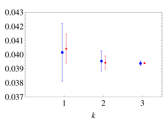
Figure 1: Results for ${\cal R}$, the QCD corrections to $R_{e^{+}e^{-}}$, in $(k+1)^{th}$ order (N^kLO) at an energy $Q/\tilde{\Lambda}_{\scriptscriptstyle{\overline{\mathrm{MS}}}}=340$. The larger points displaced leftwards are in the $\overline{\rm MS}$ scheme, while the smaller points displaced rightwards are the optimized results. In both cases the error bars correspond to $\mid\!r_{k}a^{k+1}\!\mid$.

Example 2: $Q/\tilde{\Lambda}_{\scriptscriptstyle{\overline{\mathrm{MS}}}}=68$.

Order	$a_{\scriptscriptstyle{\overline{\mathrm{MS}}}}$	$\mathcal{R}_{\scriptscriptstyle{\overline{\mathrm{MS}}}}$ series	$\mathcal{R}_{\scriptscriptstyle{\overline{\mathrm{MS}}}}$
$k=1$	$0.0507097$	$0.05(1+0.07)$	$0.05433[362]$
$k=2$	$0.0509032$	$0.05(1+0.07-0.03)$	$0.05287[169]$
$k=3$	$0.0509356$	$0.05(1+0.07-0.03-0.01)$	$0.05236[54]$
Order	$\bar{a}$	$\bar{\mathcal{R}}$ series	$\bar{\mathcal{R}}$
$k=1$	$0.0568587$	$0.06(1-0.03)$	$0.05496[190]$
$k=2$	$0.0525541$	$0.05(1-0.02+0.02)$	$0.05256[112]$
$k=3$	$0.0520416$	$0.05(1+0.002+0.003+0.002)$	$0.05245[13]$

Table 2. Results (as Table 1) for $Q/\tilde{\Lambda}_{\scriptscriptstyle{\overline{\mathrm{MS}}}}=68$.

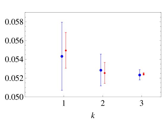
Figure 2: As Fig. 1 but for $Q/\tilde{\Lambda}_{\scriptscriptstyle{\overline{\mathrm{MS}}}}=68$.

6.3 Low-energy examples

Next we turn to lower-energy examples, where the differences between $\overline{\rm MS}$ and OPT are more dramatic. With $n_{f}=2$ the $\beta$ function’s leading coefficients are

$$b=\frac{29}{6},\quad\quad c=\frac{115}{58},$$ (6.13)

and [19, 21]

$$c_{2}^{\scriptscriptstyle{\overline{\rm MS}}}=\frac{48241}{8352}=5.77598,$$ (6.14)

$$c_{3}^{\scriptscriptstyle{\overline{\rm MS}}}=\frac{18799309}{902016}+\frac{68881}{12528}\zeta(3)=27.45054.$$ (6.15)

The ${\cal R}$ coefficients, in the $\overline{\rm MS}$ scheme, are [18, 20, 6]

$$r_{1}^{\scriptscriptstyle{\overline{\rm MS}}}=1.755117,\quad\quad r_{2}^{\scriptscriptstyle{\overline{\rm MS}}}=-9.14055,\quad\quad r_{3}^{\scriptscriptstyle{\overline{\rm MS}}}=-123.18799.$$ (6.16)

(Again, the exact values [6] were used in our calculations.) Inserting these values in Eq. (2.40) yields

$$\tilde{\rho}_{2}=-9.92498,\quad\quad\tilde{\rho}_{3}=-115.21021.$$ (6.17)

Tables 3–7 and Figures 3–7 give results at successively lower energies; $Q/\tilde{\Lambda}_{\scriptscriptstyle{\overline{\rm MS}}}=5,2,1.7,1.5$ and $0$. One sees in the $\overline{\rm MS}$ results the characteristic symptoms of an asymptotic series; after initially seeming to converge, the series starts to go bad, with the error estimate increasing with order. In Example 3 the effect is just visible in the $k=3$ result, but in Examples 4 and 5 the effect becomes more dramatic. In Example 6 there is no $k=3\,\,\,\overline{\rm MS}$ result at all since for $Q/\tilde{\Lambda}_{\scriptscriptstyle{\overline{\rm MS}}}<1.645$ there is no solution to the $k=3$ int-$\beta$ equation. At still lower values of $Q/\tilde{\Lambda}_{\scriptscriptstyle{\overline{\rm MS}}}$, below $1.396$ and $1$ respectively, the $k=2$ and $k=1$ $\overline{\rm MS}$ int-$\beta$ equations have no solution.

By contrast, the optimized results show a monotonic decrease in the expected error at higher orders. The $k=1$ results, in Examples 5 and 6 particularly, are very uncertain at low energies — indeed, for $Q/\tilde{\Lambda}_{\scriptscriptstyle{\overline{\rm MS}}}<1.438$ there is no solution to the $k=1$ optimal int-$\beta$ equation, Eq. (3.14). However, for $k=2$ and $3$ the optimized results improve very significantly. Indeed, for $k=2$ and $3$ there are optimized results down to zero energy, because the optimized $\beta$ function turns out to have a non-trivial fixed point (see Appendix B). The new $k=3$ results provide solid confirmation of the earlier $k=2$ results [3, 4, 5]. As shown in the table for example 7, the $Q=0$ result for $\bar{{\cal R}}$ improves from $0.3\pm 0.3$ to $0.2\pm 0.1$.

Example 3: $Q/\tilde{\Lambda}_{\scriptscriptstyle{\overline{\rm MS}}}=5$.

Order	$a_{\scriptscriptstyle{\overline{\rm MS}}}$	${\cal R}_{\scriptscriptstyle{\overline{\rm MS}}}$ series	${\cal R}_{\scriptscriptstyle{\overline{\rm MS}}}$
$k=1$	$0.0862557$	$0.09(1+0.15)$	$0.099[13]$
$k=2$	$0.0902494$	$0.09(1+0.16-0.07)$	$0.098[7]$
$k=3$	$0.0911287$	$0.09(1+0.16-0.08-0.09)$	$0.090[8]$
Order	$\bar{a}$	$\bar{{\cal R}}$ series	$\bar{{\cal R}}$
$k=1$	$0.117285$	$0.12(1-0.09)$	$0.106[11]$
$k=2$	$0.0952429$	$0.10(1-0.05+0.05)$	$0.095[5]$
$k=3$	$0.0899359$	$0.09(1-0.01-0.02+0.04)$	$0.091[4]$

Table 3. Results for $Q/\tilde{\Lambda}_{\scriptscriptstyle{\overline{\rm MS}}}=5$.

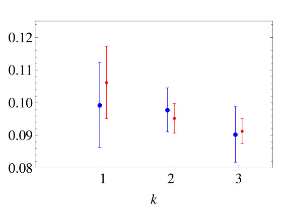
Figure 3: As Fig. 1 but for $Q/\tilde{\Lambda}_{\scriptscriptstyle{\overline{\rm MS}}}=5$.

Example 4: $Q/\tilde{\Lambda}_{\scriptscriptstyle{\overline{\rm MS}}}=2$.

Order	$a_{\scriptscriptstyle{\overline{\rm MS}}}$	${\cal R}_{\scriptscriptstyle{\overline{\rm MS}}}$ series	${\cal R}_{\scriptscriptstyle{\overline{\rm MS}}}$
$k=1$	$0.1626471$	$0.16(1+0.29)$	$0.209[46]$
$k=2$	$0.1963533$	$0.20(1+0.34-0.35)$	$0.195[69]$
$k=3$	$0.2193679$	$0.22(1+0.39-0.44-1.30)$	$-0.08\pm 0.29$
Order	$\bar{a}$	$\bar{{\cal R}}$ series	$\bar{{\cal R}}$
$k=1$	$0.3648099$	$0.36(1-0.21)$	$0.288[77]$
$k=2$	$0.1725913$	$0.17(1-0.17+0.18)$	$0.173[31]$
$k=3$	$0.1421756$	$0.14(1-0.08-0.09+0.17)$	$0.143[25]$

Table 4. Results for $Q/\tilde{\Lambda}_{\scriptscriptstyle{\overline{\rm MS}}}=2$.

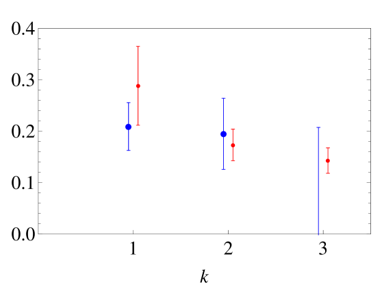
Figure 4: As Fig. 1 but for $Q/\tilde{\Lambda}_{\scriptscriptstyle{\overline{\rm MS}}}=2$. (The $k=3\,\,\,\overline{\rm MS}$ result is slightly negative; only its error bar is visible.)

Example 5: $Q/\tilde{\Lambda}_{\scriptscriptstyle{\overline{\rm MS}}}=1.7$.

Order	$a_{\scriptscriptstyle{\overline{\rm MS}}}$	${\cal R}_{\scriptscriptstyle{\overline{\rm MS}}}$ series	${\cal R}_{\scriptscriptstyle{\overline{\rm MS}}}$
$k=1$	$0.1966624$	$0.20(1+0.35)$	$0.265[68]$
$k=2$	$0.2691684$	$0.27(1+0.47-0.66)$	$0.218[178]$
$k=3$	$0.4153849$	$0.42(1+0.73-1.58-8.83)$	$-3.60\pm 3.67$
Order	$\bar{a}$	$\bar{{\cal R}}$ series	$\bar{{\cal R}}$
$k=1$	$0.6669931$	$0.67(1-0.28)$	$0.477[190]$
$k=2$	$0.1970393$	$0.20(1-0.24+0.25)$	$0.199[49]$
$k=3$	$0.1530735$	$0.15(1-0.11-0.11+0.22)$	$0.153[34]$

Table 5. Results for $Q/\tilde{\Lambda}_{\scriptscriptstyle{\overline{\rm MS}}}=1.7$.

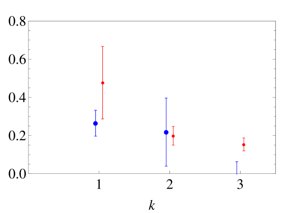
Figure 5: As Fig. 1 but for $Q/\tilde{\Lambda}_{\scriptscriptstyle{\overline{\rm MS}}}=1.7$. (Only the tip of the huge error bar for the $k=3\,\,\,\overline{\rm MS}$ result is visible.)

Example 6: $Q/\tilde{\Lambda}_{\scriptscriptstyle{\overline{\rm MS}}}=1.5$.

Order	$a_{\scriptscriptstyle{\overline{\rm MS}}}$	${\cal R}_{\scriptscriptstyle{\overline{\rm MS}}}$ series	${\cal R}_{\scriptscriptstyle{\overline{\rm MS}}}$
$k=1$	$0.236877$	$0.24(1+0.42)$	$0.335[98]$
$k=2$	$0.431322$	$0.43(1+0.76-1.70)$	$0.02\pm 0.73$
$k=3$	no solution
Order	$\bar{a}$	$\bar{{\cal R}}$ series	$\bar{{\cal R}}$
$k=1$	$2.4690661$	$2.5(1-0.42)$	$1.4\pm 1.0$
$k=2$	$0.2173977$	$0.22(1-0.31+0.33)$	$0.221[71]$
$k=3$	$0.1605183$	$0.16(1-0.13-0.13+0.26)$	$0.161[42]$

Table 6. Results for $Q/\tilde{\Lambda}_{\scriptscriptstyle{\overline{\rm MS}}}=1.5$.

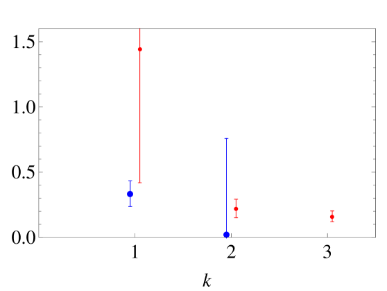
Figure 6: As Fig. 1 but for $Q/\tilde{\Lambda}_{\scriptscriptstyle{\overline{\rm MS}}}=1.5$. (There is no $k=3\,\,\,\overline{\rm MS}$ result in this case.)

Example 7: $Q/\tilde{\Lambda}_{\scriptscriptstyle{\overline{\rm MS}}}=0$  (fixed point).

Order	$\bar{a}$	$\bar{{\cal R}}$ series	$\bar{{\cal R}}$
$k=1$	no solution
$k=2$	$0.2635259$	$0.26(1-0.76+1.01)$	$0.330[267]$
$k=3$	$0.1800794$	$0.18(1-0.25-0.16+0.44)$	$0.185[79]$

Table 7. Results for the infrared fixed-point limit, $Q/\tilde{\Lambda}_{\scriptscriptstyle{\overline{\rm MS}}}=0$. There are no $\overline{\rm MS}$ results in this case.

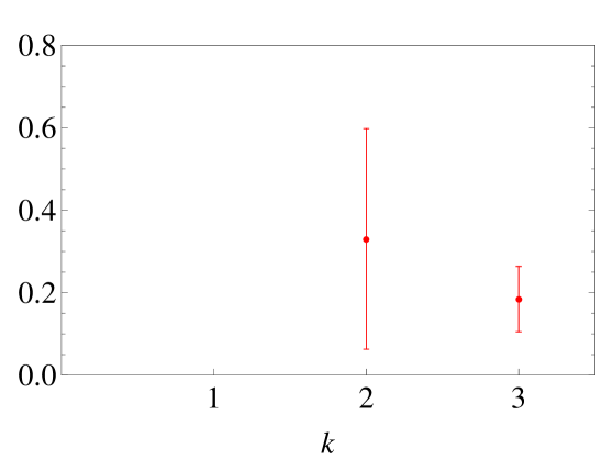
Figure 7: As Fig. 1 but for the infrared fixed-point limit, $Q/\tilde{\Lambda}_{\scriptscriptstyle{\overline{\rm MS}}}=0$. There are no $\overline{\rm MS}$ results in this case, and no $k=1$ optimized result.

7 Concluding Remarks

We first summarize the lessons of the numerical examples, which compared the $\overline{\rm MS}(\mu=Q)$ and optimized results. At moderately high energies, the differences are well within the error estimates; the main advantage of optimization here is to achieve greater precision. At low energies, however, the optimized results show steady convergence, while the $\overline{\rm MS}$ results begin to show the typical pathologies of a non-convergent asymptotic series. We can expect these pathologies to eventually show up in the $\overline{\rm MS}$ results at higher energies when the series is taken to high enough order. In this sense the low-energy examples are a “preview” of the divergent-series problems to be expected in $\overline{\rm MS}$ or any fixed RS.

Whether or not the optimized results ultimately converge is a matter of conjecture at present. However, the lessons of toy models [22, 23] and from the linear $\delta$-expansion for the anharmonic oscillator [15], together with the present results, suggest that it is a very real possibility. We should say at once that we would not expect the optimized results to converge to the exact, physical answer. We certainly expect there to be nonperturbative contributions (higher-twist terms that involve powers of $e^{-1/(ba)}$ and hence are invisible to perturbation theory). A physically defined quantity ${\cal R}$ in QCD is, in general, a sum of perturbative and nonperturbative terms, ${\cal R}_{\rm pert}+{\cal R}_{\rm nonpert}$. The issue, though, is whether this decomposition can be made unique and physically meaningful or whether it is inherently ambiguous and dependent on RS. It seems reasonable that ${\cal R}_{\rm nonpert}$ should involve only infrared physics and so should be calculable, in principle, without any essential need for renormalization. If that is so, there would have to be a version of perturbation theory that converges to a RS-invariant result, ${\cal R}_{\rm pert}$. Optimization, where at each order we demand that the result be “as RS invariant as possible,” is the natural candidate to be that version of perturbation theory — without any need to invoke extra tricks (such as Padé approximants, Borel summation, etc.).

The good convergence of the optimized results in the $e^{+}e^{-}$ case remains true even down to zero energy, where the third-order finding [3, 4, 5] of a limit ${\cal R}=0.3\pm 0.3$ is confirmed and made more precise; ${\cal R}=0.2\pm 0.1$. This result is very important because there are many indications from phenomenology (see the mini-review in Ref. [5]) that the QCD couplant does freeze at low energies. Usually freezing is something that theorists put in by hand, but here it is an outcome, a prediction. There is nothing in the optimization approach that forces freezing to occur; the fact that it does for $R_{e^{+}e^{-}}$ is due to the $\tilde{\rho}_{2},\tilde{\rho}_{3}$ values resulting from the Feynman-diagram calculations.

The methods described here could be applied to many other perturbative physical quantities. In particular, fourth-order results are now available for $\tau$-lepton and $Z^{0}$ decay widths and for some deep-inelastic-scattering sum rules [6, 36]. Previous studies of OPT applied to these quantities [3, 37, 38] could now be extended to fourth order.

We have not discussed here physical quantities that explicitly involve parton distribution functions or fragmentation functions. Such quantities are plagued by another kind of ambiguity; factorization-scheme dependence — an ambiguity similar to, and entangled with, RS dependence. The “principle of minimal sensitivity” can be applied here, too. Unfortunately, the original analysis [39] was stymied by an algebraic error, corrected later in Ref. [40] (see also [41]). These papers use the language of structure-function moments — which, while natural theoretically, is perhaps not very convenient phenomenologically. A purely numerical approach to “optimization” [42, 43] is certainly feasible, but laborious. It would be valuable to somehow reformulate Ref. [40]’s results in a way that would combine easily with practical methods for using and empirically determining parton distribution functions. We suspect, based on the important results of [42, 43], that several important QCD cross sections are currently underestimated, and that “optimization” could significantly reduce the theoretical uncertainties of many others.

Acknowledgments

I am grateful to T. J. Sarkar for discussions that were helpful in refining the solution for the optimized coefficients. I also thank Tal Einav for detailed comments on an early version of the manuscript.

Appendix A: Proof of the “complete sum” identity

This appendix provides a proof of the identity, mentioned in subsection 4.3, for the “complete sum:”

$$\sum_{j=0}^{k}\,c_{j}a^{j}\left(\frac{i-j-1}{i+j-1}\right)B_{i+j}(a)=1\quad\quad\quad i=(1),2,\ldots,k.$$ (A.1)

From the definition of the $\beta_{j}(a)$ and $B_{j}(a)$ functions we have Eqs. (2.19) and (2.20). Substituting into the l.h.s. of (A.1) yields

$$\frac{B(a)}{a^{i-1}}\sum_{j=0}^{k}\,c_{j}(i-j-1)\int_{0}^{a}\!dx\frac{x^{i+j-2}}{B(x)^{2}}.$$ (A.2)

Pulling the integration outside the sum and re-grouping leads to

$$\frac{B(a)}{a^{i-1}}\int_{0}^{a}\!dx\frac{x^{i-2}}{B(x)^{2}}\left((i-1)\sum_{j=0}^{k}c_{j}x^{j}-\sum_{j=0}^{k}jc_{j}x^{j}\right).$$ (A.3)

The integrand can now be recognized as

$$\frac{x^{i-2}}{B(x)^{2}}\left((i-1)B(x)-x\frac{dB(x)}{dx}\right)=\frac{d}{dx}\left(\frac{x^{i-1}}{B(x)}\right),$$ (A.4)

so the integral can be done immediately, giving

$$\frac{B(a)}{a^{i-1}}\left[\frac{x^{i-1}}{B(x)}\right]_{x=0}^{x=a}.$$ (A.5)

For $i>1$ the lower endpoint ($x=0$) makes no contribution, so the result is unity, as claimed.

The case $i=1$ requires special treatment. As in the definition of $H_{1}(a)$, Eqs. (4.3,  4.4), we should interpret the $i=1$ case of Eq. (A.1) above as

$$B(a)-\sum_{j=1}^{k}c_{j}a^{j}B_{j+1}(a)=1.$$ (A.6)

The proof parallels the steps above except that there is now a contribution from the $x=0$ endpoint that results in the cancellation of the $B(a)$ term.

Appendix B: Infrared limit and fixed-point behaviour

In asymptotically free theories, perturbation theory works best at high energies. By investigating low energies we can learn important lessons about how perturbation theory can go bad, and why RS choice is crucial. As the physical scale $Q$ is lowered, and the effective couplant grows, we can expect the physical quantity ${\cal R}$ to either (i) go to infinity at some finite energy of order $\tilde{\Lambda}$, or (ii) tend to a finite limit as $Q\to 0$. The latter scenario is usually said to happen if and only if the $\beta$ function has a zero at some finite $a=a^{*}$, called a “fixed point.” That statement, however, is too naive because “the $\beta$ function” is not a unique object; it depends on RS.

At second order in QCD, for $n_{f}\!\leq\!8$, the $\beta$ function has no non-zero fixed point in any RS. At higher orders, though, the question depends entirely on the RS choice. In the $\overline{\rm MS}$ scheme the $c_{2}$ and $c_{3}$ coefficients are positive, so no fixed point exists and $\overline{\rm MS}$ results, at third and fourth orders, go to infinity at some $Q$ of order $\Lambda_{{\scriptscriptstyle{\overline{\rm MS}}}}$. However, the optimization procedure does give finite results at arbitrarily low energies in the $e^{+}e^{-}$ case. At third order [5] ${\cal R}(e^{+}e^{-})$ approaches a finite limit, $0.3\pm 0.3$. At fourth order we find $0.2\pm 0.1$. These results can be found by applying the algorithm of Section 5 at lower and lower $Q$, but can also be obtained much more simply because [24] the optimization equations greatly simplify at a fixed point. The results of Ref. [24] (converting notation: $\rho_{2}^{\rm old}=\tilde{\rho}_{2}-{\scriptstyle{\frac{1}{4}}}c^{2}$ and $\rho_{3}^{\rm old}={\scriptstyle{\frac{1}{2}}}\tilde{\rho}_{3}$) are as follows. At third order the optimized $a^{*}$ is given by the smallest root of the quadratic equation

$$\frac{7}{4}+ca^{*}+3\left(\tilde{\rho}_{2}-\frac{1}{4}c^{2}\right){a^{*}}^{2}=0,$$ (B.1)

and the limiting value of ${\cal R}^{(3)}$ is

$${{\cal R}^{*}}^{(3)}=a^{*}\left(\frac{7}{6}+\frac{1}{6}ca^{*}\right).$$ (B.2)

At fourth order the corresponding equations are

$$\frac{83}{64}+\frac{13}{16}ca^{*}+\frac{3}{4}\tilde{\rho}_{2}{a^{*}}^{2}+2\tilde{\rho}_{3}{a^{*}}^{3}=0,$$ (B.3)

and

$${{\cal R}^{*}}^{(4)}=a^{*}\left(\frac{249}{256}+\frac{13}{64}ca^{*}+\frac{1}{16}\tilde{\rho}_{2}{a^{*}}^{2}\right).$$ (B.4)

The fixed-point limit of Eq. (4.13), the new formula for the $s_{m}\equiv\left(\frac{m+{\scriptstyle{{\rm P}}}}{{\scriptstyle{{\rm P}}}}\right)r_{m}$ coefficients, can be written as

$$\hat{s}_{m}=\frac{1}{(k-1)}\left[(k-2m-1)\hat{t}_{m}-(k-2m)\hat{t}_{m-1}\right],$$ (B.5)

or, equivalently,

$$\hat{s}_{m}=\frac{1}{(k-1)}\left[(k-2m)\hat{c}_{m}-\hat{t}_{m}\right],$$ (B.6)

where $\hat{s}_{m}\equiv s_{m}{a^{*}}^{m}$, and $\hat{c}_{m}\equiv c_{m}{a^{*}}^{m}$, and $\hat{t}_{m}$ is a partial sum of $\beta$-function terms:

$$\hat{t}_{m}=\sum_{i=0}^{m}c_{j}{a^{*}}^{j}.$$ (B.7)

These new formulas simplify the task of generalizing Ref. [24]’s results to higher orders.

The occurrence of a fixed point is not inevitable in OPT; the $a^{*}$ equation, (B.1) or (B.3), may or may not have a positive, real root. A small positive $a^{*}$ is found for ${\cal R}(e^{+}e^{-})$, for $n_{f}=2$, because the invariants $\tilde{\rho}_{2}$ and $\tilde{\rho}_{3}$ are negative and sizeable. Interestingly, for $n_{f}$ above about $6$ (depending on the assumed electric charges of the extra quarks) one does not find a solution to Eq. (B.3). However, a finite infrared limit still exists, but it occurs by a new mechanism; we hope to report on this phenomenon in a future publication.

References

- [1] P. M. Stevenson, Phys. Rev. D 23, 2916 (1981).
- [2] E. C. G. Stueckelberg and A. Peterman, Helv. Phys. Acta 26, 449 (1953); M. Gell Mann and F. Low, Phys. Rev. 95, 1300 (1954).
- [3] J. Chýla, A. Kataev, and S. A. Larin, Phys. Lett. B 267, 269 (1991).
- [4] A. C. Mattingly and P. M. Stevenson, Phys. Rev. Lett. 69, 1320 (1992).
- [5] A. C. Mattingly and P. M. Stevenson, Phys. Rev. D 49, 437 (1994).
- [6] P. A. Baikov, K. G. Chetyrkin, J. H. Kühn, and J. Rittinger, Phys. Lett. B 714, 62 (2012); P. A. Baikov, K. G. Chetyrkin, and J. H. Kühn, Phys. Rev. Lett. 101, 012002 (2008).
- [7] P. M. Stevenson, Nucl. Phys. B 203, 472 (1982).
- [8] P. M. Stevenson in Perturbative Quantum Chromodynamics (Tallahassee, 1981), ed. D. W. Duke and J. F. Owens (AIP, New York, 1981).
- [9] P. M. Stevenson, in Radiative Corrections in , ed. B. W. Lynn and J. F. Wheater (World Scientific, Singapore, 1984).
- [10] W. Celmaster and P. M. Stevenson, Phys. Lett. B 125, 493 (1983); J. Chýla, Phys. Lett. B 356, 341 (1995).
- [11] W. Caswell, Ann. Phys. (N.Y.) 123, 153 (1979); J. Killingbeck, J. Phys. A 14, 1005 (1981); E. J. Austin and J. Killingbeck, ibid. 15, L443 (1982).
- [12] J. M. Rabin, Nucl. Phys. B 224, 308 (1983).
- [13] S. K. Kauffmann and S. M. Perez, J. Phys. A 17, 2027 (1984).
- [14] H. F. Jones and M. Monoyios, Int. J. Mod. Phys. A 4, 1735 (1989); J. O. Akeyo and H. F. Jones, ibid., 1668; J-H. Pei, C. M. Dai, and D. S. Chuu, Surf. Sci. 222 1 (1989); P. M. Stevenson, Phys. Rev. D 24, 1622 (1981).
- [15] I. R. C. Buckley, A. Duncan, and H. F. Jones, Phys. Rev. D 47, 2554 (1993); A. Duncan and H. F. Jones, ibid., 2560; C. M. Bender, A. Duncan and H. F. Jones, ibid., 49, 4219 (1994); C. Arvantis, H. F. Jones, and C. S. Parker, ibid., 52, 3704 (1995); R. Guida, K. Konishi, and H. Suzuki, Ann. Phys. 241, 152 (1995); ibid., 249, 109 (1996); H. Kleinert and V. Schulte-Frohlinde, Critical Properties of Theories, Chap. 19 (World Scientific, Singapore, 2001).
- [16] H. D. Politzer, Phys. Rev. Lett. 30, 1346 (1973); D. J. Gross and F. Wilczek, ibid. 30, 1343 (1973); G. ’t Hooft, report at the Marseille Conference Yang-Mills Fields, 1972.
- [17] D. R. T. Jones, Nucl. Phys. B 75, 531 (1974); W. Caswell, Phys. Rev. Lett. 33, 244 (1974); E. S. Egorian and O. V. Tarasov, Theor. Mat. Fiz. 41, 26 (1979).
- [18] K. G. Chetyrkin, A. L. Kataev, and F. V. Tkachov, Phys. Lett. B 85, 277 (1979); M. Dine and J. Sapirstein, Phys. Rev. Lett. 43, 668 (1979); W. Celmaster and R. J. Gonsalves, Phys. Rev. D 21, 3112 (1980).
- [19] O. V. Tarasov, A. A. Vladimirov, and A. Yu. Zharkov, Phys. Lett. B 93, 429 (1980); S. A. Larin and J. A. M. Vermaseren, Phys. Lett. B 303, 334 (1993).
- [20] L. R. Surguladze and M. A. Samuel, Phys. Rev. Lett. 66, 560 (1991); S. G. Gorishny, A. L. Kataev, and S. A. Larin, Phys. Lett. B 259, 144 (1991).
- [21] T. van Ritbergen, J. A. M. Vermaseren, and S. A. Larin, Phys. Lett. B 400, 379 (1997).
- [22] P. M. Stevenson, Nucl. Phys. B 231, 65 (1984).
- [23] K. Van Acoleyen and H. Verschelde, Phys. Rev. D 69 125006 (2004).
- [24] J. Kubo, S. Sakakibara, and P. M. Stevenson, Phys. Rev. D 29, 1682 (1984).
- [25] G. ’t Hooft, Lecture at 1977 Coral Gables Conf., Orbis Scientiae.
- [26] A. J. Buras, E. G. Floratos, D. A. Ross, and C. T. Sachrajda, Nucl. Phys. B 131, 308 (1977); W. A. Bardeen, A. J. Buras, D. W. Duke, and T. Muta, Phys. Rev. D 18, 3998 (1978).
- [27] G. Dissertori and G. P. Salam, “Quantum Chromodynamics” review in K. Nakamura et al. (Particle Data Group), J. Phys. G 37, 075021 (2010).
- [28] D. W. Duke and R. G. Roberts, Phys. Rep. 120, 275 (1985).
- [29] W. Celmaster and R. J. Gonsalves, Phys. Rev. D 20, 1420 (1979).
- [30] G. Grunberg, Phys. Rev. D 29, 2315 (1984).
- [31] P. M. Stevenson, Phys. Rev. D 33, 3130 (1986).
- [32] E. Monsay and C. Rosenzweig, Phys. Rev. D 23, 1217 (1981).
- [33] M. R. Pennington, Phys. Rev. D 26, 2048 (1982); J. C. Wrigley, Phys. Rev. D 27, 1965 (1983); See also P. M. Stevenson, ibid., 27, 1968 (1983); J. A. Mignaco and I. Roditi, Phys. Lett. B 126, 481 (1983).
- [34] W. J. Marciano, Phys. Rev. D 29, 580 (1984).
- [35] E. C. Poggio, H. R. Quinn, and S. Weinberg, Phys. Rev. D 13, 1958 (1976).
- [36] P. A. Baikov, K. G. Chetyrkin, and J. H. Kühn, Phys. Rev. Lett. 104, 132004 (2010); hep-ph/1201.5804.
- [37] A. C. Mattingly, hep-ph/9402230 (1994).
- [38] J. Chýla and A. L. Kataev, Phys. Lett. B 297, 385 (1992); in Report of the Working Group on Precision Calculations for the Resonance (CERN Yellow Report), ed. D. Yu. Bardin, G. Passarino, and W. Hollik.
- [39] H. D. Politzer, Nucl. Phys. B 194, 493 (1982).
- [40] P. M. Stevenson and H. D. Politzer, Nucl. Phys. B 277, 758 (1986).
- [41] H. Nakkagawa, A. Niégawa, and H. Yokota, Phys. Rev. D 34, 244 (1986).
- [42] P. Aurenche, R. Baier, and M. Fontannaz, Z. Phys. C 48, 143 (1990); P. Aurenche, R. Baier, M. Fontannaz, J. F. Owens, and M. Werlen, Phys. Rev. D 39, 3275 (1989).
- [43] J. Chýla, JHEP 03, 042 (2003) [arXiv:hep-ph/0303179]; J. Srbek and J. Chýla arXiv:hep-ph/0504089; M. J. Dinsdale, arXiv:hep-ph/0512069 (2005).