Attractor networks and memory replay of phase coded spike patterns

Abstract

We analyse the storage and retrieval capacity in a recurrent neural network of spiking integrate and fire neurons. In the model we distinguish between a learning mode, during which the synaptic connections change according to a Spike-Timing Dependent Plasticity (STDP) rule, and a recall mode, in which connections strengths are no more plastic. Our findings show the ability of the network to store and recall periodic phase coded patterns a small number of neurons has been stimulated. The self sustained dynamics selectively gives an oscillating spiking activity that matches one of the stored patterns, depending on the initialization of the network.

, and

Introduction

In many areas of the brain, with different brain functionality, it has been recently hypothesized that spike phase (i.e. the relative phases of the spikes of neurons participating to a collective oscillation, or the phases of spikes relatively to the ongoing oscillation) play a crucial role in coding information, together with the conventional spike rate code. Experimental evidence of the importance of spike phases in neural coding starts with the first experiments on theta phase precession in rat’s place cells [1, 2], showing that both spike rate and spike phase are correlated with rat’s position. In addition to this, several experiments on short-term memory of multiple objects in prefrontal cortices of monkeys [3] supported the hypothesis that collective oscillations may underlie a phase-dependent neural coding and that the distinct phase alignment of information relative to population oscillations may play a role for disambiguating individual short-term memory items. hypothesis are also pointed out in the experiments on spike-phase coding of natural stimuli in auditory and visual primary cortex [4, 5].
In particular the path-integration system and the hippocampal and entorhinal cortex circuit, that forms a spatial map of the environment, has been deeply investigated [1, 2, 6], showing that the place cells and grid cells form a map in which precise phase relationship among units play a critical role. The oscillators interference models [7, 8] of path-integration are based on the integration of animal velocity by phase of oscillator cells (such as a theta cell whose frequency is modulated by the animals’ velocity), and the read-out of this phase by interference between different oscillators. In the paper of Blair et al. [7], for example, the rate-coded position information of the grid cells comes from a set of theta oscillatory cells whose frequency is precisely modulated by the rat’s movements’ velocity. Different sets of such theta cells are needed, with cells in different sets have different frequency, and cells in each set have a different phase relationships each other. Moreover, since phase angles between different theta oscillators encode the rat’s position, the oscillators must maintain stable phase relationships with one other over behaviorally relevant time scales (many seconds, or dozens of theta cycle periods). Hence, oscillatory interference models impose strict constraints upon the dynamical properties of theta oscillators. It is not presently known whether these constraints are satisfied by theta-generating circuits in the rat brain, and if so, how.

In this paper we present a possibility to build a circuit in which stable phase relationships between spikes of different neurons are maintained in a robust way with respect to noise. This feature is due to the robustness of the dynamical attractors with respect to noise, which are also stable across the changes of frequency. Indeed the collective frequency of the circuit depends on the firing threshold $\Theta$ and the phase relationships among units in the circuit is maintained when output global frequency of the circuit is changed, indeed it is the phase relationship that is a dynamical attractor of the circuit and not the absolute spike timing difference among units. The mechanism of storing information in the specific spike pattern of activity and recall info by recalling the specific spike alignment (or spike phase in case of periodic spatiotemporal pattern) may be a useful mechanism as substrate for memory. The importance of precise timing relationships among neurons, which may carry information to be stored, is supported also by the evidence that precise timing of few milliseconds is able to change the sign of synaptic plasticity. The dependence of synaptic modification on the precise timing and order of pre- and postsynaptic spiking has been demonstrated in a variety of neural circuits of different species. Many experiments show that a synapse can be potentiated or depressed depending on the relative timing of the pre- and post-synaptic spikes. This timing dependence of magnitude and sign of plasticity, observed in several types of cortical [10, 11, 12] and hippocampal [12, 13, 15] neurons, is usually termed Spike Timing Dependent Plasticity or STDP. Here, we face the role of a learning rule based on STDP in storing multiple phase-coded memories as attractor states of the neural dynamics.The spatio-temporal patterns are periodic sequences of spikes, whose features are encoded in the phase shifts between firing neurons.
We use an Integrate-and-Fire (IF) neuronal model, namely in a Spike-Response Model (SRM) formulation, which is very popular for theoretical studies on populations of neurons, especially for large-scale simulations. This simple choice is suitable to study the storage and retrieve capability of the network, instead of focusing on the complexity of the neuronal structure. Once performed the learning stage, we examine the network capability to replay(retrieve) a stored pattern. Partial presentation of a pattern, i.e. short externally induced spike sequences, with phases similar to the ones of the stored phase pattern, induces the network to retrieve selectively the stored item, as far as the number of stored items is not larger then the network storage capacity. If the network retrieves one of the stored items, the neural population spontaneously fires with the specific phase alignments of that pattern, until external input does not change the state of the network.

1 Learning with Spike-Timing Dependent Plasticity

In the experiment of Markram [10] it was reported that if the pre-synaptic spike repeatedly precedes a post- synaptic action potential within a short time window (10 -20 ms), the synapse is potentiated (Long Term Potentiation, LTP). If the opposite occurs, the synapse undergoes depression (Long Term Depression, LTD). Both effects are combined in a synapse equipped with STDP [16, 15, 13, 14, 10, 11], where the degree of change in synaptic strength depends on the delay between pre and post-synaptic spikes, via a learning window that is temporally asymmetric (see Fig. 1). In our model we consider a recurrent neural network with $N(N-1)$ possible connections $J_{ij}$, where $N$ is the number of neural units. The connections $J_{ij}$, during the learning mode, are subject to plasticity and change their efficacy according to a learning rule inspired to the STDP. After the learning stage, the collective dynamics is studied.
According to the learning model already introduced in [19, 18, 17], the change in the connection $J_{ij}$ that occurs in the time interval $[-T,0]$ due to periodic spike trains can be formulated as follows:

$$\delta J_{ij}\propto\int\limits_{-T}^{0}dt\int\limits_{-T}^{0}dt^{\prime}\,y_{i}(t)A(t-t^{\prime})y_{j}(t^{\prime})$$ (1)

where $y_{j}(t)$ is the activity of the pre-synaptic neuron at time t, and $y_{i}(t)$ the activity of the post-synaptic one. It means that the probability that unit $i$ has a spike in the interval $(t,t+\Delta t)$ is proportional to $y_{i}(t)\Delta t$ in the limit $\Delta t\to 0$. The learning window A($\tau=t-t^{\prime}$) is the measure of the strength of synaptic change when a time delay $\tau$ occurs between pre and post-synaptic train. To model the experimental results of STDP, the learning window $A(\tau)$ should be an asymmetric function of $\tau$, mainly positive (LTP) for $\tau>0$ and mainly negative (LTD) for $\tau<0$.
While Eqn. (1) holds for activity pattern $y(t)$ which represents instantaneous firing rate and it has been studied in a analog rate model [19, 18, 17] and in a spin network model [26], here we want to study the case of spiking neurons. Therefore, the patterns to be stored are defined as precise periodic sequence of spikes. Namely, the activity of the neuron $j$ is a spike train at times $t^{\mu}_{j}$,

$$y_{j}^{\mu}(t)=\sum_{n}\delta(t-(t^{\mu}_{j}+nT^{\mu})),$$ (2)

where $t^{\mu}_{j}+nT^{\mu}$ is the set of spike times of unit j in the pattern $\mu$ with period $T^{\mu}$. Therefore the change in the connection $J_{ij}$ during the learning of pre-synaptic and post-synaptic spike trains of the periodic pattern $\mu$, is given, following Eqn. 1, by

$$J_{ij}^{\mu}=\sum_{n}A(t^{\mu}_{j}-t^{\mu}_{i}+nT^{\mu}).$$ (3)

           Figure 1: a) Plot of the learning window $A(\tau)$ used in the learning rule (see Eqs. (1), (2), (3)) to model STDP. Parameters of the function (see Eqn. (4)) fit the experimental data of [13].

The window $A(\tau)$ that we use, shown in Fig. 1, is given by

$$A(\tau)=a_{p}e^{-\tau/T_{p}}-a_{D}e^{-\eta\tau/T_{p}}\;\textrm{for}\;\tau>0\;\textrm{and}\;A(\tau)=a_{p}e^{\eta\tau/T_{D}}-a_{D}e^{\tau/T_{D}}\;\textrm{for}\;\tau<0,$$ (4)

with the same parameters used in [20] to fit the experimental data of [13], $a_{p}=\gamma\,[1/T_{p}+\eta/T_{D}]^{-1}$, $a_{D}=\gamma\,[\eta/T_{p}+1/T_{D}]^{-1}$, with $T_{p}=10.2$ ms, $T_{D}=28.6$ ms, $\eta=4$, $\gamma=42$. This function satisfies the balance condition $\int_{-\infty}^{\infty}A(\tau)d\tau=0$.
Writing Eqn. (1)-(2), implicitly we have assumed that, with periodic spike trains used to induce plasticity, the effects of all separate spike pairs sum linearly with the STDP kernel shown in Fig. 1. Note that this rule is valid only when, as here, simple periodic spike trains are used to induce plasticity, and in a proper range of frequency. Timing-dependent learning curves as shown in Fig. 1 are indeed typically measured by giving a sequence of 100 pairs of spikes repeatedly, with fixed frequency in a proper range. In fact, pairing single presynaptic and postsynaptic spikes, or pairing at very low frequency (1Hz) led to an LTD-only STDP kernel [27]. Similarly, pairing at high enough frequencies [12] the timing-dependent rule becomes LTP-only, i.e., both positive and negative timings produce LTP. Moreover the number of pairing also can change the bidirectional kernel shape into a LTP-only shape. In particular, for arbitrary non-periodic spike trains major nonlinearities arise from the history of spike activity, also on timescales longer than the width of the STDP curve (see [9] and reference therein). The simple model that we use here, Eqn. 3, is enough to describe the plasticity that occurs when long periodic spike trains with frequency in a proper range is used. At very low, as well as very high frequency, and with few spike pairs, the timing dependence of plasticity is not well described by the bidirectional kernel shown in Fig. 1, and a more detailed model is needed to account for integration of spike pairs when not-periodic arbitrary trains are used [9].

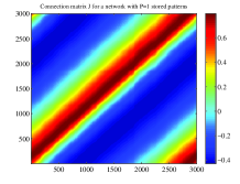
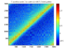
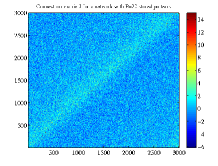
Figure 2: Visual representation of the connection matrix $J_{ij}$ resulting from network with N=3000 units and P stored patterns at $\omega_{\mu}=20Hz$. Left P=1, middle P=2, right P=20.

The spike spatiotemporal patterns that we study in this paper are periodic spatiotemporal patterns of spikes, with phases of spike $\phi^{\mu}_{j}$ randomly chosen from a uniform distribution in $[0,2\pi)$. Namely, the set of timing of spikes of unit $j$ can be noted as $\quad t^{\mu}_{j}+nT^{\mu}=(\phi^{\mu}_{j}+2\pi n)/\omega_{\mu}$, $\omega_{\mu}/2\pi$ is the oscillation frequency of the neurons. Thus, each pattern $\mu$ is defined by its frequency $\omega_{\mu}/2\pi$, and by the specific phases of spike $\phi^{\mu}_{j}$ of the neurons $j=1,..,N$.
Therefore, the change in the connection $J_{ij}$ provided by the learning of pattern $\mu$ is given by

$$J_{ij}^{\mu}=\sum_{n}A(t^{\mu}_{j}-t^{\mu}_{i}+nT^{\mu})=\sum_{n}A(\phi^{\mu}_{j}/\omega_{\mu}-\phi^{\mu}_{i}/\omega_{\mu}+2\pi n/\omega_{\mu}).$$ (5)

In each pattern, information is coded in the precise time delay between unit $i$ and unit $j$ spikes, that corresponds to a precise phase relationship among the unit $i$ and $j$, therefore this kind of spatiotemporal patterns is often called phase coded pattern. When we store multiple phase coded patterns defined in (2), with $\mu=1,2,\ldots,P$, the learned connections are the sum of the contributions from individual patterns, namely

$$J_{ij}=\sum_{\mu=1}^{P}J^{\mu}_{ij}.$$ (6)

The connection matrix $J_{ij}$ coming out from Eqn. (3) and (5) at $\omega_{\mu}=20Hz$ and $\phi^{\mu}_{i}$ randomly chosen in $[0,2\pi]$, is shown in Fig. 2 for P=1, P=2 and P=20. The units $i,j$ on the axes are sorted according to the value of $\phi^{1}_{i}$ of first pattern $\mu=1$. With P=1 it’s clearly visible the structure of the connectivity matrix, however note that even at P=20, when the correlation structure of the connectivity matrix with the stored patterns is not visible, the network is still able to selectively retrieve each of the P stored patterns, in a range of neuronal threshold values such that storage capacity is equal or higher then 20.

2 Model Dynamics

We distinguish a learning mode in which plasticity rule (3), (4) and (5) is used to store P phase-coded pattern into the network connectivity, from a dynamic mode (or retrieval mode) in which connections $J_{ij}$ are fixed to the value found after learning (Eqn. (5)) and the dynamics of the neurons is studied. Therefore we simulate a Leaky Integrate and Fire network, with fixed connections. The Leaky Integrate and Fire model of single neuron is given by a simple Spike-Response-Model formulation (SRM) introduced by Gernster in [21, 22]. While integrate-and-fire models are usually defined in terms of differential equations, the SRM expresses the membrane potential at time $t$ as an integral over the past. When membrane potential reach a threshold $\Theta$ a spike is scheduled. This allows us to use a event-driven programming and makes the numerical simulations faster with respect to a differential equation formulation. In its simplified version [21], the SRM₀ model, where neuronal refractoriness is not taken into account, the internal state of a spiking neuron depends on the last output spike and on the total postsynaptic potential. Supposing the membrane resting potential is set to zero after a spike, neglecting the shape of the spiking pulse, the postsynaptic membrane potential is given by:

$$h_{i}(t)=\sum_{j}J_{ij}\sum_{\hat{t_{j}}}\epsilon(t-\hat{t_{j}}),$$ (7)

where the sum over $\hat{t_{j}}$ runs over all presynaptic firing times. The function $\epsilon$ describe the response kernel to incoming spikes on neuron $i$. Namely, each presynaptic spike $j$, with arrival time $\hat{t_{j}}$, is supposed to add to the membrane potential a postsynaptic potential of the form $J_{ij}\epsilon(t-\hat{t_{j}})$, where

$$\epsilon(t-\hat{t_{j}})=K\left[\exp\left(-\frac{t-\hat{t_{j}}}{\tau_{m}}\right)-\exp\left(-\frac{t-\hat{t_{j}}}{\tau_{s}}\right)\right]H(t-\hat{t_{j}})$$ (8)

where $\tau_{m}$ is the membrane time constant (here 10 ms), $\tau_{s}$ is the synapse time constant (here 5 ms), $H$ is the Heaviside step function, and K is a multiplicative constant chosen so that the maximum value of the kernel is 1. The sign of the synaptic connection $J_{ij}$ set the sign of the postsynaptic potential’s change. When the postsynaptic potential of neuron $i$ reaches the threshold $\Theta$, a postsynaptic spike is scheduled, and postsynaptic potential is reset to the resting value zero. Note that a change of $\Theta$ in our model may correspond to a change in the value of spiking threshold of the units, or to a global change in the scaling factor of synaptic connections $J_{ij}$ since what matters is the ratio $J_{ij}/\Theta$. Anyway a lower value of $\Theta$ correspond to a higher excitability of the network. We simulate this simple model with $J_{ij}$ taken from the learning rule given by Eqn. (5)-(6), with $P$ patterns in a network of $N$ units.
In the following, the network capacity is analyzed considering the maximum number of patterns that the network is able to perfectly recall. In particular we investigate the role of two parameters of the model: the frequency of the stored patterns $\omega_{\mu}$, and the firing threshold $\Theta$ which change the excitability of the network.

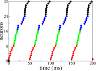
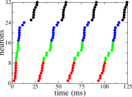
a)  b)  c) 

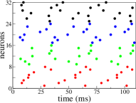
Figure 3: Dynamics of a network with $N=3000$ neurons and connections given by Eqn. (6) with $P=5$ and $\omega_{\mu}=20$ Hz. A subset of 32 neurons is chosen and sorted by increasing values of phase $\phi_{i}^{1}$ of the stored pattern $\mu=1$. Different colors refer to phase values belonging to different phase intervals of pattern $\mu=1$: $(0-\pi/2)$ red, $(\pi/2-\pi)$ green, $(\pi-3/2\pi)$ blue,$(3/2\pi-2\pi)$ black . The stored pattern is shown in a), plotting the times $(\phi_{i}^{1}+2\pi n)/\omega_{1}$. Hence, the generated dynamics when a short train of $M=300$ spikes is induced on the network, corresponding to the pattern $\mu=1$ in b) and $\mu=2$ in c). Figure b) shows that when the network dynamic is stimulated by a partial cue of pattern $\mu=1$, the neurons oscillate with phase alignments resembling pattern $\mu=1$, but at different frequency. Otherwise, in c), when the partial cue is taken from pattern $\mu=2$, the neurons phase relationships, even if periodic, are uncorrelated with pattern $\mu=1$, and recall the phase of pattern $\mu=2$.

3 Storage capacity analysis

We did numerical simulations of the SRM network described in Eqn. (8)-(9) with $N=3000$ neurons, and connections $J_{ij}$ given by (5) with different number of patterns P. After the learning process, to check if it’s possible to recall one of the encoded patterns, we give an initial signal equal to $M\ll N$ spikes, taken from the stored pattern $\mu$, and we check that after this short signal the spontaneous dynamics of the network gives sustained activity with spikes aligned to the phases $\phi_{i}^{\mu}$ of pattern $\mu$. During the retrieval mode, connections strength is no more plastic as it happens for the learning mode. This distinction in two stages (learning and retrieval), even though is not well assessed in real neural dynamics, is useful to simplify the analysis and also finds some neurophysiological motivations [23, 24]. An example of successful selective retrieval process is shown in Fig. 3 where, depending on the partial cue presented to the network, the phase of firing neurons resemble one or another of the stored patterns. The network dynamic is initially stimulated by an initial short train of $M=300$ spikes (10% of the network) chosen at times $t^{\mu}_{i}$ from pattern $\mu=1,2$ and we check if this initial train triggers the sustained replay of pattern $\mu=1,2$ at large times. We introduce a quantitative similarity measure to estimate the overlap between the network activity during the spontaneous dynamics and the stored phase-coded pattern, defined as

$$|m^{\mu}(t)|=\left|\frac{1}{N}\sum_{j=1,\ldots,N}e^{-i2\pi t_{j}^{*}/T^{*}}e^{i\phi_{j}^{\mu}}\right|$$ (9)

where $t_{j}^{*}$ is the spike timing of neuron $j$ during the spontaneous dynamics, and $T^{*}$ is an estimation of the period of the collective spontaneous dynamics. The overlap in Eqn. (9) is equal to $1$ when the phase-coded pattern is retrieved perfectly (even thou with a different time scale), while is $\simeq 1/\sqrt{N}$ when phases of spikes are uncorrelated to the stored phases.

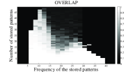
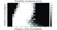
a) b) c)

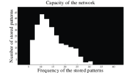
Figure 4: Capacity estimation of a network made up of 3000 neurons. In order to verify that recall of a stored pattern is correct, we compared the phases of pattern $\mu=1$ with spontaneous network dynamic stimulated by 300 spikes chosen at times $t^{1}_{i}$ ($i=1\ldots 300$). The firing neuronal firing threshold, $\Theta_{n}=170$. For each boxes in the figure the y-axis represent the number of stored patterns and x-axis is the frequency of the stored patterns $\omega_{\mu}/2\pi$. In a) the overlap measure defined in Eqn. (9) is shown in a black and white color legend: the brighter is the color the higher is the overlap $|m^{\mu}(t)|$. b) Probability of sustained activity with the same color legend used for the overlap. In c) the effective capacity of the network is shown, i.e. a pattern is considered perfectly retrieved once the product of the overlap with the probability of sustained activity is higher than 0.5.

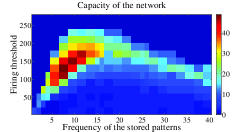
a) b)

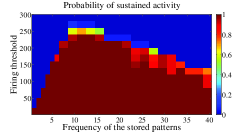
Figure 5: a) Summary of the network capacity as a function of the frequency and firing threshold. The color legend shows the number of correctly stored pattern. b) Probability of self-sustained activity for a network with P=3 stored patterns in the plane $(\omega,\Theta)$. The color legend shows the region of the plane where a pattern could be stored.

The Figure 4 shows results of numerical simulations averaged over 50 runs, namely for different implementations of the network and patterns to be stored. The overlap $|m^{\mu}(t)|$ is reported in Fig. 4a in a black and white colored legend, along with the probability of self-sustained activity, Fig. 4b as a function of $\omega_{\mu}$ at fixed firing threshold ($\Theta=170$). This gives an indication of whether or not the initial stimulating spikes are sufficient to generate a persistent spontaneous oscillatory activity regardless of the phases alignment between neurons. In our analysis we did not considered the non-persistent activity, that is the spontaneous dynamic occurring in a short transient time, right after the initial stimulating spikes. This means that black colored areas in Fig. 4 are not necessarily associated with an absence of spontaneous activity, but only to an absence of long term activity. Hence, we consider a successful pattern replay when the overlap, weighted with the probability of long term sustained activity, is larger than 0.5. This is reported in Fig. 4c, where we observe a large interval of frequency with a good storage capacity.
We also investigate the role of the firing threshold $\Theta$. Note that changing $\Theta$ in our model may correspond to a change excitability. i.e a change of firing threshold or in global change in the synaptic connections $J_{ij}$. Indeed, the working range of the network depends on both the frequency of the stored pattern, as well as on the threshold $\Theta$. The capacity of the network is summarized in Fig. 5, where we report, in the plane frequency-threshold $(\omega,\Theta)$, the number of perfectly replayed pattern (Fig. 5a) and the probability of sustained activity (Fig. 5b).
Another important result is observed looking at neurons firing activity. In Fig. 6 we see that by lowering the threshold $\Theta$ below an optimal value, a burst of activity takes place within each cycle, with phases aligned with the pattern. This open the possibility to have a coding scheme in which the phases encode pattern’s information, and rate in each cycle represents the strength and saliency of the retrieval or it may encode another variable. The recall of the same phase-coded pattern with different number of spikes per cycle accords well with recent observation of Huxter et al. [25] in hippocampal place cells, showing occurrence of the same phases with different rates. They show that the phase of firing and firing rate are dissociable and can represent two independent variables, e.g. the animals location within the place field and its speed of movement through the field. The number of spikes per cycle as a function of the threshold $\Theta$ is reported in Fig 7a, where a dependence on the frequency of the replayed pattern is also observed in the plane frequency-threshold.

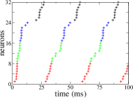
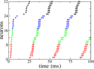
a)  b)  c) 

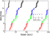
Figure 6: Recall of the pattern $\mu=1$ for networks of 3000 neurons having different values of parameter $\Theta$, namely $\Theta=100$ in a), $\Theta=60$ in b) and $\Theta=20$ in c). Depending on the value of $\Theta$, the phase-coded pattern is replayed with a different number of spikes per cycle.

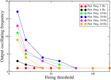
a)  b) 

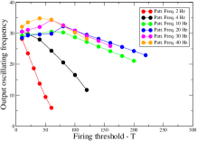
Figure 7: (a) The number of spikes per cycle as a function of the firing threshold $\Theta$ for a network with one encoded pattern, at different frequencies $\omega_{\mu}/2\pi$. (b) The network oscillating frequencies as function of the firing threshold. A stored pattern is replayed at frequencies which slowly decays with increasing $\Theta$ for most of the pattern frequencies $\omega_{\mu}/2\pi$.

Lastly, in Fig. 7b, the dependence of the output frequency of collective oscillations is studied as a function of $\Theta$. Notably, the stored phase-coded patterns are replayed in a compressed time scale for $\omega^{\mu}/2\pi<30$ Hz.

4 Conclusions

We studied the storage and replay properties of a network of spiking integrate and fire neurons, whose learning mechanism is based on the Spike-Timing Dependent Plasticity. The encoded patterns are periodic spike sequences, whose features are encoded in the relative phase shifts between neurons. The proposed associative memory approach, that replay the stored sequence, can be a method for recognize an item, by activating the same memorized pattern in response of a similar input, or could be a method to transfer the memorized item to another area of the brain (such as for memory consolidation during sleep). We systematically quantify and compare the retrieval capacity of the network by changing two parameters of the model: the frequency of the input (encoding) patterns, $\omega/2\pi$, and the neuronal firing threshold, $\Theta$. The response of the network changes by changing those parameters which, however, are not the only ones governing the spiking activity of neurons. Future works will consider a further analysis of the model parameters and wheter to tune them to modify the network capability in a controlled manner.

References

- [1] O’Keefe J., Recce M.L. (1993). Phase relationship between hippocampal place units and the EEG theta rhythm. Hippocampus, Vol 3, 317-330.
- [2] O’Keefe J., Burgess N. (2005). Dual phase and rate coding in hippocampal place cells: theoretical significance and relationship to entorhinal grid cells. Hippocampus, 15(7):853-866.
- [3] Siegel M., Warden M.R., and Miller E.K. (2009). Phase-dependent neuronal coding of objects in short-term memory. PNAS 106, 21341-21346.
- [4] Montemurro M.A., Rasch M.J., Murayama Y., Logothetis N.K., Panzeri S. (2008). Phase-of-Firing Coding of Natural Visual Stimuli in Primary Visual Cortex. Current Biology, Volume 18, Issue 5, 375-380.
- [5] Kayser C., Montemurro M.A., Logothetis N.K., Panzeri S. (2009). Spike-Phase Coding Boosts and Stabilizes Information Carried by Spatial and Temporal Spike Patterns. Neuron, Vol. 61, Issue 4, 597-608.
- [6] Geisler C., Robbe D., Zugaro M., Sirota A., Buzsaki G. (2007). Hippocampal place cell assemblies are speed-controlled oscillators. PNAS.
- [7] Blair H.T.,Gupta K., Zhang K. (2008). Conversion of a phase- to a rate-coded position signal by a three-stage model of theta cells, grid cells, and place cells. Hippocampus, Vol. 18 (12), 1239-1255.
- [8] Burgess N., Barry C., O’Keefe J. (2007). An oscillatory interference model of grid cell firing. Hippocampus, Vol. 17, 801-812.
- [9] Shouval H.Z., Wang S.S., Wittenberg G.M. (2010). Spike timing dependent plasticity: a consequence of more fundamental learning rules. Frontiers in Computational Neuroscience, 4, 19.
- [10] Markram H., Lubke J., Frotscher M., Sakmann B. (1997). Regulation of synaptic efficacy by coincidence of postsynaptic APs and EPSPs. Science, 275, 213-215.
- [11] Feldman D.E. (2000). Timing-based LTP and LTD and vertical inputs to layer II/III pyramidal cells in rat barrel cortex. Neuron 27, 45-56.
- [12] Sjostrom P.J., Turrigiano G., Nelson S.B. (2001). Rate, Timing, and Cooperativity Jointly Determine Cortical Synaptic Plasticity. Neuron, 32, 1149-1164.
- [13] Bi G.Q., and Poo M.M. (1998). Precise spike timing determines the direction and extent of synaptic modifications in cultured hippocampal neurons. J. Neurosci. 18, 10464:10472.
- [14] Bi G.Q., and Poo M.M. (2001). Synaptic modification by correlated activity: Hebb’s postulate revisited. Annual Review Neuroscience 24, 139-166.
- [15] Debanne D., Gahwiler B.H. and Thompson S.M. (1998).event driven programming Long-term synaptic plasticity between pairs of individual CA3 pyramidal cells in rat hippocampal slice cultures. J. Physiol. 507, 237-247.
- [16] Magee J.C., and Johnston D. (1997). A synaptically controlled associative signal for Hebbian plasticity in hippocampal neurons. Science 275, 209-212.
- [17] Yoshioka M., Scarpetta S., Marinaro M. (2007). Spatiotemporal learning in analog neural networks using spike-timing-dependent synaptic plasticity. Phys. Rev. E, 75, 051917.
- [18] Scarpetta S., Zhaoping L., Hertz J. (2002). Hebbian Imprinting and Retrieval in Oscillatory Neural Networks. Neural Computation, Vol. 14(10), 2371-96.
- [19] Scarpetta S., Zhaoping L., Hertz J. (2001). Spike-Timing-Dependent Learning for Oscillatory Networks. NIPS, Vol. 13, MIT Press.
- [20] Abarbanel H., Huerta R., Rabinovich M.I. (2002) Dynamical model of long-term synaptic plasticity. Proc. Nas. Acad. Sci. 99, n.15, 10132-10137.
- [21] Gerstner W., Kistler W. (2001) Spiking neuron models: single neurons, populations, plasticity Cambridge University Press, New York, NY.
- [22] Gerstner W., Ritz R., van Hemmen J.L. (1993). Why spikes? Hebbian learning and retrieval of time-resolved excitation patterns. Biological Cybernetics 69(5-6), 503-515.
- [23] Hasselmo M.E. (1993). Acetylcholine and learning in a cortical associative memory. Neural Computation 5, p.32-44.
- [24] Hasselmo M.E. (1999). Neuromodulation: acetylcholine and memory consolidation. Trend in Cognitive Sciences 3(9) 351.
- [25] Huxter J., Burgess N., O’Keefe J. (2003). Independent rate and temporal coding in hippocampal pyramidal cells. Nature 425, 828-32.
- [26] Scarpetta S., Antonio de Candia A., Giacco F. (2010). Storage of phase-coded patterns via STDP in fully-connected and sparse network: a study of the network capacity. Frontiers in synaptic neuroscience 2, 1-12.
- [27] Wittenberg G.M., Wang S.S. (2006). Malleability of spike-timing-dependent plasticity at the CA3-CA1 synapse. Journal of Neuroscience, 26, 6610-6617.