Vortexje - An Open-Source Panel Method for Co-Simulation

Abstract

This paper discusses the use of the 3-dimensional panel method for dynamical system simulation. Specifically, the advantages and disadvantages of model exchange versus co-simulation of the aerodynamics and the dynamical system model are discussed. Based on a trade-off analysis, a set of recommendations for a panel method implementation and for a co-simulation environment is proposed. These recommendations are implemented in a C++ library, offered on-line under an open source license. This code is validated against XFLR5, and its suitability for co-simulation is demonstrated with an example of a tethered wing, i.e, a kite. The panel method implementation and the co-simulation environment are shown to be able to solve this stiff problem in a stable fashion.

1 Introduction

This paper focuses on the application of the 3-dimensional panel method [13, 17, 8, 15] to simulation of dynamical systems interacting with fluid flow. The primary advantage of such a potential flow method over numerical solution of the Navier-Stokes equations is the ease by which the panel equations can be solved numerically. A panel method has unknowns on the surface of the immersed body only, whereas numerical solution of the Navier-Stokes equations requires a 3-dimensional mesh throughout the region of flow. This reduced computational requirement renders the panel method a viable candidate for dynamic simulation.

On the other hand, the standard panel method is restricted to the modelling of inviscid, incompressible, and irrotational flows. This implies that the unmodified panel method is only applicable to subsonic flows at angles of attack where flow separation does not occur. Even under these circumstances, the standard panel method does not predict viscuous drag. Nevertheless, the panel method has turned out to be a valuable tool for aerodynamic analysis [8, 15], and extensions have been developed to incorporate viscosity effects [8].

Other 3-dimensional potential flow methods, such as the vortex-lattice and lifting-line methods, share the same assumptions of inviscid, incompressible, and irrotational flow [15]. These methods, however, introduce the further assumption of an infinitely thin airfoil. For this reason we will not consider these methods further, and focus our attention on the 3-dimensional panel method.

Our aim lies in the development of an open-source implementation of the panel method specifically designed for dynamical system simulation, where the aerodynamic forces and moments interact with the system dynamics. An example of such a system is a wing tethered to the ground, i.e., a kite. We use the panel method to obtain the aerodynamic forces and moments acting on the kite, and an ODE solver to compute the shape and tension of the tether. The aerodynamic forces of the kite act on the tether, and the other way around. We use this stiff interaction as a test problem for the development of a panel method and dynamical system simulation methodology.

Our approach based on the panel method stands in contrast to the approach taken in [6], where a kite is discretized into multiple bodies. In the multi-body approach, the aerodynamics for each body are independent, and prescribed by the modeller. When the panel method is used, the computed aerodynamic forces and moments result from the shape of the entire wing, its orientation in the flow, and its interaction with the wake. Results obtained from the panel method can therefore be expected to be more accurate.

In the next section, we start by outlining the basic ideas underlying the panel method.

2 The Panel Method

Let a body be immersed in a flow with velocity field $\vec{v}$. The panel method models flows that are irrotational. Irrotationality means that, outside of the body and inside of the flow,

$$\nabla\times\vec{v}=\vec{0},$$

or, equivalently [20],

$$\vec{v}=\nabla\phi,$$ (1)

for some potential function $\phi$.

In our application, we furthermore assume the flow to be incompressible, as is applicable for subsonic flows [15]:

$$\nabla\cdot\vec{v}=0.$$ (2)

Substituting Equation 1 into Equation 2, we find that the potential function satisfies the Laplace equation:

$$\nabla^{2}\phi=0.$$ (3)

The panel method arrives at a solution of the Laplace equation by summing up certain elementary solutions located on the body boundary. In our implementation, we use the elementary solutions known as the source and the doublet [15].

Taking the gradient of the potential, we obtain the velocity field. From the velocity field, in turn, an application of the Bernoulli equation yields the pressure distribution.

The source and doublet elementary solutions are weighted such that, firstly, on the boundary there results no flow velocity normal to it, and secondly, that the resulting potential is zero on the body interior. To make this proceduce suitable for a digital computer, we discretize the body and its wake into a number of panels. We then assign each panel both a source as well as a doublet weight variable, labeled $\sigma$ and $\mu$, respectively. This results in the so-called source and doublet distributions. The weight assignment conditions, finally, translate into an asymmetric system of linear equations. For further details, we refer the reader to [15].

3 Existing Open-Source Panel Method Implementations

The XFLR5 package [9] is the only available open-source implementation of the 3-dimensional source-doublet panel method that the author is aware of. Unfortunately, XFLR5 features a tight integration between the method implementation and the user interface. The user interface is designed for the analysis of fixed flight conditions. To use the underlying method implementation for dynamic simulation, it would need to be separated from the rest of the code base. This would be an unpractical and time-consuming process.

Instead of going through such a process of scavenging bits and pieces from the XFLR5 code base, we choose to start from a clean slate. In this way we ensure that the code follows our design goals, rather than the other way around. Furthermore, we aim to design the implementation such that a graphical user interface could readily be built using our implementation as a reusable component. This stands in contrast to XFLR5, where the user interface is an integral and hard-to-separate part of the package.

4 Use Case: A Tethered Wing

During the last two decades, kites, i.e. tethered wings, have gained popularity not only for sports, but also for the towing of ships [18], and for the generation of wind energy on land [16, 7]. In our case we investigate the kite as it poses a stiff simulation problem, and therefore a challenge for our simulation paradigm. We will use a kite simulation to validate our design decisions.

We model the kite aerodynamics using the panel method, and the tether as a string of point-masses connected by high-modulus spring-dampers, represented by an ODE. The aerodynamic forces acting on the kite, resulting from the panel method, are added to the spring-damper forces of the top point-mass in the tether model – see Figure 1. In this way the bulk of the kite’s lift force is balanced by the line forces. As a consequence, the aerodynamic forces and the kinematics operate on different orders of magnitude, resulting in a stiff interaction.

We generated a mesh for a typical C-shaped surf kite with the geometry specified in Table 1. The resulting mesh is shown in Figure 1.

Parameter	Value
Airfoil	Clark-Y
Aspect ratio	$6.0$
Projected aspect ratio	$4.5$
Tip alignment	Trailing edge
Root chord	$3$ m
Tip/chord ratio	$0.25$
Airfoil panels	$18$
Spanwise panels	$18$
Tether attachment point	$0.75$ m from leading edge
Mass	$6.0$ kg
Yawing inertia	$5.0$ kg $\cdot$ m2

Table 1: Kite parameters

Figure 1: Kite and tether simulation. The yawing direction of the kite is indicated with the dotted arrow.

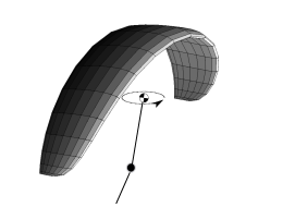
Such surf kites yaw around their tether (cf. Figure 1) in response to asymmetrical deformations [6]. To obtain such asymmetrical states, we set up the following dynamic deformation in the spanwise coordinate $z_{b}$:

$$\Delta z_{b}=ux_{b},$$

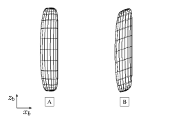
where $x_{b}$ is a dimensionless chordwise coordinate between 0 and 1. This simplified deformation is inspired by the observation that the tips of arc-shaped kites bend inward when pulling on their respective steering lines. In order to focus on the essentials, we neglect any further deformation in the normal direction.

The steering input $u$ is commanded as a single scalar input variable. The top view of an undeformed mesh, and of a deformed mesh with a steering input of $u=1$, is displayed in Figure 2.

Figure 2: Kite mesh without steering deformation (A) and with steering deformation $u=1$ (B). Top view.

Further deformation as well as viscuous effects are neglected. While viscuous drag is crucial in obtaining an accurate model, in this work we are primarily interested in obtaining a rudimentary model suitable for testing our simulation setup. Empirically identified viscuous drag may be added to the equations of motion in the dynamical system simulation.

The equations of the tether model are trivial but space-consuming. For this reason, we do not include them in the present paper. The full equations can be obtained from the author on request.

5 Model Exchange versus Co-Simulation

In the present section we discuss two different practices that can be used to integrate the panel method with a dynamical system simulator. Of primary importance is the distinction between the so-called model exchange and co-simulation paradigms [5].

Model exchange refers to the practice of wrapping an external model in a stateless function, evaluated as part of an ODE or DAE. The external model thereby becomes a part of a containing dynamical system model. In our case, any states such as the source and doublet distributions, would become part of the system of equations. We note that these states must indeed be stored, as a proper use of the unsteady Bernoulli equation does require knowledge of the time-variation of the source and doublet distributions. The disadvantage of model exchange for the panel method is that the size of the system matrix would grow quadratically in the number of panels. Furthermore, all but the most trivial solvers would make repeated calls to the panel method function. This would pose a performance problem due to the overhead of solving the – usually large – linear system for computing the doublet distribution.

A co-simulation master, on the other hand, manages two different simulation environments, each with their own internal states. The co-simulation master coordinates the interaction between the simulation environments at pre-defined events or times. The simulators are commanded to step forward in turns [5]. In a co-simulation environment, a panel method simulator is able to maintain internal states without expanding the system matrices of the dynamical system simulator.

Stiff interactions between the panel method and the dynamical system simulator pose a challange for both concepts. In a model exchange environment, performance of the overall system solver would be limited by an implicit solver evaluating the panel method Jacobian using finite differences. The same holds for co-simulation context, where in this case a specialized implicit co-simulation solver would need to be developed in addition.

Comparing our two options we see that both suffer from the panel method’s linear system overhead equally. Co-simulation, however, does not suffer from quadratic growth of the system matrix. This advantage compels us to focus on the co-simulation paradigm.

6 Panel Method API Design

As our focus lies with dynamic simulation, rather than with highly detailed aerodynamic analysis, we implement a classical first-order source-doublet panel method as described in [16]. For computation of the surface velocities we follow the treatment of N. Marcov [11], and for 3-D mesh generation we follow the algorithm detailed in [8].

Furthermore, during a dynamic simulation a body may find itself interacting with its own wake. Therefore we supplement the classical method with singularity elimination following Dixon [10].

For now, we will not consider aeroelastacity and boundary layer models. We may, however, add such features in the future.

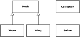
We will now briefly discuss the considerations leading to our software architecture. In order to facilitate a modular description of an object in flow, we choose to allow for a multitude of meshes to be specified. Wake-emitting, wake, and source-only meshes are allowed. In line with the common approach of modeling an airplane as consisting of wake-emitting and source-only parts [8, 15], we choose to implement an additional class for collecting a multitude of meshes. In this way, the programmer may handle the airplane as one, applying transformations to the collection as if it were a single object. These design considerations are shown in the diagram shown in Figure 3.

Figure 3: Class diagram.

The classes were implemented in C++ in a library called Vortexje, available on-line [3] under the terms of an open-source license. Its sole dependency, aside from a C++ compiler, is the Eigen [12] template library for linear algebra. Vortexje uses the Bi-CGSTAB [21] implementation from Eigen [12] to solve the doublet coefficient equations. An example code using the library is listed on the Vortexje website [3].

In the next section we compare simulation results from Vortexje and XFLR5 for a simple example, before, in the section thereafter, embarking on a co-simulation of a kite with its tether.

7 Validation

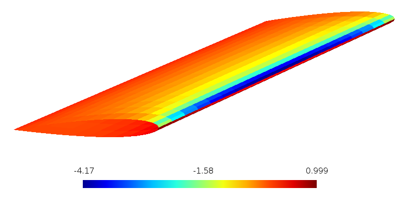
To validate our implementation, we simulate a simple reference wing using both XFLR5 (in inviscid mode) and Vortexje. Since the use of XFLR5 is well-established, we expect it to compute the pressure distribution on our reference wing correctly. For this reason, we test the pressure distribution and resulting aerodynamic coefficients computed by Vortexje against those computed by XFLR5.

Our reference wing is specified in Table 2. The pressure distribution of this wing, computed by Vortexje at an angle of attack of $10$ degrees, is shown in Figure 4. A comparison of the integrated pressure distributions of XFLR5 and Vortexje is shown in Figure 5.

Parameter	Value
Airfoil	NACA0012
Span	$6$ m
Chord	$1$ m
Airfoil panels	$32$
Spanwise panels	$40$
Airspeed	$30$ m/s
Fluid density	$1.2$ kg/m3

Table 2: Validation set-up.

Figure 4: Pressure distribution, as computed by Vortexje.

Figure 5: Comparison of XFLR5 and Vortexje simulation results.

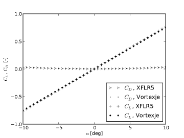
On closer inspection of the subtle differences shown in Figure 5, we find that XFLR5 computes the potential gradient on the wing surface as the gradient of the doublet distribution:

$$\vec{v}(\vec{x})=-(\nabla\mu)(\vec{x}).$$

This assumption originates from [17], where it is stated without proof. We, on other hand, implemented N. Marcov’s formula [11], which derives an alternative expression for the surface-derivative of the potential:

$$\vec{v}(\vec{x})=\vec{w}(\vec{x})-\frac{1}{2}(\nabla\mu)(\vec{x}),$$ (4)

with the term $\vec{w}(\vec{x})$ representing the Cauchy principal value of the potential gradient contribution of the entire boundary. To compute this value numerically, we sum up the potential gradients of all panels, treating the local panel the same as all others. We do not run into the theoretical singularity this way, as the explicit expressions of the potential gradients for source and doublet panels are singular only on panel boundaries [15]. The theoretical singularity of the local potential contribution at the point of evaluation, however, is significant, and gives rise to the second term in Equation 4.

There is one more difference in implementation. This pertains the so-called far-field formulas [15]. The far-field formulas are computationally inexpensive approximations of the panel potential contributions for points far away from the respective panel. Our omission of the far-field formulas is likely to share responsiblity for the subtle divergence in results of Figure 5.

Based on the fact that the observed differences are extremely small, we consider Vortexje to have passed our validation test for the reference wing. Furthermore, our implementation rests on a mathematically underpinned surface-derivative formula, and its results may therefore be more reliable than those provided by XFLR5.

8 Co-Simulation Methodology

We now return to co-simulation, and verify our approach with our case problem, the tethered kite.

For encoding the tether ODE, we selected Modelica for its ease of use and extensibility. As the bulk of the computational time will be spent in the ODE and panel method solvers, we choose to implement the co-simulation master in the Python scripting language. The JModelica project [1] maintains an open-source Python package for simulating model exchange Functional Mock-up Units (FMUs), PyFMI [5].

We also use JModelica to compile the tether model to an FMU, and use PyFMI to access the FMU from Python. JModelica’s Assimulo package – which wraps the SUNDIALS suite of integrators [14] – is used to integrate the tether model.

To the upper end of the tether, we attach a kite mesh with predefined deformation states in C++. The presence of multiple lines is emulated by prescribing zero roll and pitch angles with respect to the tether. The yaw angle, on the other hand, is determined by the aerodynamic moments acting on the kite mesh. See Figure 1.

The interaction between kite and tether might, in theory, be handled using a Functional Mock-up Interface (FMI) co-simulator. As of this writing, however, PyFMI does not support the FMI co-simulation standard. Instead, we use a Boost.Python [19] class to set up communication between Python and Vortexje. Figure 6 summarizes the complete set-up.

Figure 6: Co-simulation architecture.

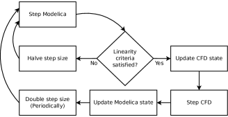
Both simulators are stepped in turn. The step size $h$ is reduced on a binary logarithmic scale until roughly linear behaviour is achieved:

$$\frac{\left|\|y(t+h)-y(t)\|-\|\dot{y}\|h\right|}{\|\dot{y}\|h}<\varepsilon,$$

where $y$ denotes the state of the dynamical system, and $\varepsilon$ is a pre-defined linearity tolerance value. The step size reduction is carried out down to a minimum step size $h_{0}$. Every $T_{h}$ time steps the step size is doubled, up to a maximum step size $h_{1}$, before entering the step size reduction algorithm. In this way, we ensure that the simulator does not remain stuck with a very small step size after integrating an interval of high stiffness, while at the same time refraining from trying an excessively large step size in vain too often. This stepping scheme is summarized as a flow chart in Figure 7. The parameters values selected for the solver are shown in Table 3.

Figure 7: Co-simulation flow chart.

Setting	Value
Minimum master step size $h_{0}$	$1\times 10^{-6}$
Maximum master step size $h_{1}$	$5\times 10^{-3}$
Step size doubling period $T_{h}$	$10$
Linearity tolerance $\varepsilon$	$0.1$
SUNDIALS solver	CVODE
CVODE absolute tolerance	$1\times 10^{-6}$
CVODE relative tolerance	$1\times 10^{-6}$
Bi-CGSTAB maximum iterations	$20\times 10^{3}$
Bi-CGSTAB tolerance	$1\times 10^{-10}$

Table 3: Solver parameters.

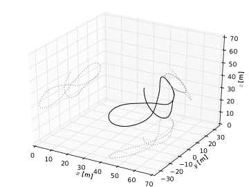
With the control algorithm from [4, 2] and an environmental wind velocity of $6$ m/s, the trajectory of the kite is shown in Figure 8. The “tail” in said figure is the arc traced from the initial point to the target trajectory. No numerical instability was observed.

Figure 8: Co-simulated kite trajectory.

9 Conclusions and Future Directions

In this work we proposed a design for a panel method implementation capable of efficient co-simulation. The design was implemented in a C++ code, released on-line under an open-source license. We continued with validation results, followed by an analysis of a co-simulation of a kite with its tether. This tether is composed of point-masses and spring-dampers, and the interaction of the spring-damper and aerodynamic kite forces results in a stiff problem. We showed that our co-simulation framework – implemented entirely using open-source software – is able to solve the kite problem in a stable fashion.

Future work will focus on adding optional aeroelasticity and boundary layer simulation features to the software. We invite interested readers to evaluate our software, and hope to establish a community of users and developers.

References

- [1] J. Åkesson, M. Gäfvert, and T. Tummescheit. JModelica - an open source platform for optimization of Modelica models. In Proceedings of MATHMOD 2009 - 6th Vienna International Conference on Mathematical Modelling, Vienna, 2009.
- [2] J. H. Baayen. Trajectory tracking control of kites with system delay, 2012, arXiv:1212.6388.
- [3] J. H. Baayen. Vortexje: Source-doublet panel method library. http://www.baayen-heinz.com/vortexje, 2012.
- [4] J. H. Baayen and W. J. Ockels. Tracking control with adaption of kites. IET Journal of Control Theory & Applications, 6(2):182–191, 2012.
- [5] T. Blochwitz, M. Otter, J. Akesson, M. Arnold, C. Clauß, H. Elmqvist, M. Friedrich, A. Junghanns, J. Mauss, D. Neumerkel, et al. Functional Mockup Interface 2.0: The standard for tool independent exchange of simulation models. In 9th International Modelica Conference, Munich, 2012.
- [6] J. Breukels. An Engineering Methodology for Kite Design. PhD thesis, Delft University of Technology, Delft, 2011.
- [7] M. Canale, L. Fagiano, and M. Milanese. Power kites for wind energy generation. IEEE Control Systems Magazine, 27(6):25–38, 2007.
- [8] T. Cebeci. An engineering approach to the calculation of aerodynamic flows. Springer, New York, 1st edition, 1999.
- [9] A. Deperrois. XFLR5. http://www.xflr5.com/, 2012.
- [10] K. Dixon, C. S. Ferreira, C. Hofemann, G. van Bussel, and G. van Kuik. A 3d unsteady panel method for vertical axis wind turbines. In The proceedings of the European Wind Energy Conference & Exhibiti on EWEC Brussels, pages 1–10, 2008.
- [11] L. Dragoş. Mathematical methods in aerodynamics. Kluwer Academic Publishers, Dordrecht, 1st edition, 2010.
- [12] G. Guennebaud, B. Jacob, et al. Eigen v3. http://eigen.tuxfamily.org, 2012.
- [13] J. L. Hess and A. M. O. Smith. Calculation of potential flow about arbitrary bodies. Progress in Aeronautical Sciences, 8:1–138, 1967.
- [14] A.C. Hindmarsh, P.N. Brown, K.E. Grant, S.L. Lee, R. Serban, D.E. Shumaker, and C.S. Woodward. SUNDIALS: Suite of nonlinear and differential/algebraic equation solvers. ACM Transactions on Mathematical Software, 31(3):363–396, 2005.
- [15] J. Katz and A. Plotkin. Low-Speed Aerodynamics. Cambridge University Press, Cambridge, 2nd edition, 2001.
- [16] M. L. Loyd. Crosswind kite power. Journal of Energy, 4(3):106–111, 1980.
- [17] B. Maskew. Program VSAERO theory document: A computer program for calculating nonlinear aerodynamic characteristics of arbitrary configurations. Technical report, NASA, 1987.
- [18] P. Naaijen, V. Koster, and R. P. Dallinga. On the power savings by an auxiliary kite propulsion system. International shipbuilding progress, 53(4):255–279, 2006.
- [19] R. Rivera, B. Dawes, and D. Abrahams. Boost. C++ libraries. http://www.boost.org, 2012.
- [20] W. Rudin. Principles of mathematical analysis. McGraw-Hill, Inc., New York, 3rd edition, 1964.
- [21] H.A. Van der Vorst. Bi-CGSTAB: A fast and smoothly converging variant of Bi-CG for the solution of nonsymmetric linear systems. SIAM Journal on Scientific and Statistical Computing, 13(2):631–644, 1992.