Clustering hidden Markov models with variational HEM

Abstract

The hidden Markov model (HMM) is a widely-used generative model that copes with sequential data, assuming that each observation is conditioned on the state of a hidden Markov chain. In this paper, we derive a novel algorithm to cluster HMMs based on the hierarchical EM (HEM) algorithm. The proposed algorithm i) clusters a given collection of HMMs into groups of HMMs that are similar, in terms of the distributions they represent, and ii) characterizes each group by a “cluster center”, i.e., a novel HMM that is representative for the group, in a manner that is consistent with the underlying generative model of the HMM. To cope with intractable inference in the E-step, the HEM algorithm is formulated as a variational optimization problem, and efficiently solved for the HMM case by leveraging an appropriate variational approximation. The benefits of the proposed algorithm, which we call variational HEM (VHEM), are demonstrated on several tasks involving time-series data, such as hierarchical clustering of motion capture sequences, and automatic annotation and retrieval of music and of online hand-writing data, showing improvements over current methods. In particular, our variational HEM algorithm effectively leverages large amounts of data when learning annotation models by using an efficient hierarchical estimation procedure, which reduces learning times and memory requirements, while improving model robustness through better regularization.

Keywords: Hierarchical EM algorithm, clustering, hidden Markov model, hidden Markov mixture model, variational approximation, time-series classification

1 Introduction

The hidden Markov model (HMM) (Rabiner and Juang, 1993) is a probabilistic model that assumes a signal is generated by a double embedded stochastic process. A discrete-time hidden state process, which evolves as a Markov chain, encodes the dynamics of the signal, while an observation process encodes the appearance of the signal at each time, conditioned on the current state. HMMs have been successfully applied to a variety of fields, including speech recognition (Rabiner and Juang, 1993), music analysis (Qi et al., 2007) and identification (Batlle et al., 2002), online hand-writing recognition (Nag et al., 1986), analysis of biological sequences (Krogh et al., 1994), and clustering of time series data (Jebara et al., 2007; Smyth, 1997).

This paper is about clustering HMMs. More precisely, we are interested in an algorithm that, given a collection of HMMs, partitions them into $K$ clusters of “similar” HMMs, while also learning a representative HMM “cluster center” that concisely and appropriately represents each cluster. This is similar to standard k-means clustering, except that the data points are HMMs now instead of vectors in $\mathbb{R}^{d}$.

Various applications motivate the design of HMM clustering algorithms, ranging from hierarchical clustering of sequential data (e.g., speech or motion sequences modeled by HMMs  (Jebara et al., 2007)), to hierarchical indexing for fast retrieval, to reducing the computational complexity of estimating mixtures of HMMs from large datasets (e.g., semantic annotation models for music and video)  — by clustering HMMs, efficiently estimated from many small subsets of the data, into a more compact mixture model of all data. However, there has been little work on HMM clustering and, therefore, its applications.

Existing approaches to clustering HMMs operate directly on the HMM parameter space, by grouping HMMs according to a suitable pairwise distance defined in terms of the HMM parameters. However, as HMM parameters lie on a non-linear manifold, a simple application of the k-means algorithm will not succeed in the task, since it assumes real vectors in a Euclidean space. In addition, such an approach would have the additional complication that HMM parameters for a particular generative model are not unique, i.e., a permutation of the states leads to the same generative model. One solution, proposed by Jebara et al. (2007), first constructs an appropriate similarity matrix between all HMMs that are to be clustered (e.g., based on the Bhattacharya affinity, which depends non-linearly on the HMM parameters (Jebara et al., 2004)), and then applies spectral clustering. While this approach has proven successful to group HMMs into similar clusters (Jebara et al., 2007), it does not directly address the issue of generating HMM cluster centers. Each cluster can still be represented by choosing one of the given HMMs, e.g., the HMM which the spectral clustering procedure maps the closest to each spectral clustering center. However, this may be suboptimal for some applications of HMM clustering, for example in hierarchical estimation of annotation models. Another distance between HMM distributions suitable for spectral clustering is the KL divergence, which in practice has been approximated by sampling sequences from one model and computing their log-likelihood under the other (Juang and Rabiner, 1985; Zhong and Ghosh, 2003; Yin and Yang, 2005).

Instead, in this paper we propose to cluster HMMs directly with respect to the probability distributions they represent. The probability distributions of the HMMs are used throughout the whole clustering algorithm, and not only to construct an initial embedding as in (Jebara et al., 2007). By clustering the output distributions of the HMMs, marginalized over the hidden-state distributions, we avoid the issue of multiple equivalent parameterizations of the hidden states. We derive a hierarchical expectation maximization (HEM) algorithm that, starting from a collection of input HMMs, estimates a smaller mixture model of HMMs that concisely represents and clusters the input HMMs (i.e., the input HMM distributions guide the estimation of the output mixture distribution).

The HEM algorithm is a generalization of the EM algorithm — the EM algorithm can be considered as a special case of HEM for a mixture of delta functions as input. The main difference between HEM and EM is in the E-step. While the EM algorithm computes the sufficient statistics given the observed data, the HEM algorithm calculates the expected sufficient statistics averaged over all possible observations generated by the input probability models. Historically, the first HEM algorithm was designed to cluster Gaussian probability distributions (Vasconcelos and Lippman, 1998). This algorithm starts from a Gaussian mixture model (GMM) with $K^{(b)}$ components and reduces it to another GMM with fewer components, where each of the mixture components of the reduced GMM represents, i.e., clusters, a group of the original Gaussian mixture components. More recently, Chan et al. (2010a) derived an HEM algorithm to cluster dynamic texture (DT) models (i.e., linear dynamical systems, LDSs) through their probability distributions. HEM has been applied successfully to construct GMM hierarchies for efficient image indexing (Vasconcelos, 2001), to cluster video represented by DTs (Chan et al., 2010b), and to estimate GMMs or DT mixtures (DTMs, i.e., LDS mixtures) from large datasets for semantic annotation of images (Carneiro et al., 2007), video (Chan et al., 2010b) and music (Turnbull et al., 2008; Coviello et al., 2011).

To extend the HEM framework for GMMs to mixtures of HMMs (or hidden Markov mixture models, H3Ms), additional marginalization over the hidden-state processes is required, as with DTMs. However, while Gaussians and DTs allow tractable inference in the E-step of HEM, this is no longer the case for HMMs. Therefore, in this work, we derive a variational formulation of the HEM algorithm (VHEM), and then leverage a variational approximation derived by Hershey et al. (2008) (which has not been used in a learning context so far) to make the inference in the E-step tractable. The resulting algorithm not only clusters HMMs, but also learns novel HMMs that are representative centers of each cluster. The resulting VHEM algorithm can be generalized to handle other classes of graphical models, for which exact computation of the E-step in the standard HEM would be intractable, by leveraging similar variational approximations — e.g., the more general case of HMMs with emission probabilities that are (mixtures of) continuous exponential family distributions.

Compared to the spectral clustering algorithm of (Jebara et al., 2007), the VHEM algorithm has several advantages that make it suitable for a variety of applications. First, the VHEM algorithm is capable of both clustering, as well as learning novel cluster centers, in a manner that is consistent with the underlying generative probabilistic framework. In addition, since it does not require sampling steps, it is also scalable with low memory requirements. As a consequence, VHEM for HMMs allows for efficient estimation of HMM mixtures from large datasets using a hierarchical estimation procedure. In particular, intermediate HMM mixtures are first estimated in parallel by running the EM algorithm on small independent portions of the dataset. The final model is then estimated from the intermediate models using the VHEM algorithm. Because VHEM is based on maximum-likelihood principles, it drives model estimation towards similar optimal parameter values as performing maximum-likelihood estimation on the full dataset. In addition, by averaging over all possible observations compatible with the input models in the E-step, VHEM provides an implicit form of regularization that prevents over-fitting and improves robustness of the learned models, compared to a direct application of the EM algorithm on the full dataset. Note that, in contrast to (Jebara et al., 2007), VHEM does not construct a kernel embedding, which is a costly operation that requires calculating of $O((K^{(b)})^{2})$ pairwise similarity scores between all input HMMs to form the similarity matrix, as well as the inversion of this matrix.

In summary, the contributions of this paper are three-fold: i) we derive a variational formulation of the HEM algorithm for clustering HMMs, which generates novel HMM centers representative of each cluster; ii) we evaluate VHEM on a variety of clustering, annotation, and retrieval problems involving time-series data, showing improvement over current clustering methods; iii) we demonstrate in experiments that VHEM can effectively learn HMMs from large sets of data, more efficiently than standard EM, while improving model robustness through better regularization. With respect to our previous work, the VHEM algorithm for H3M was originally proposed in (Coviello et al., 2012a)

The remainder of the paper is organized as follows. We review the hidden Markov model (HMM) and the hidden Markov mixture model (H3M) in Section 2. We present the derivation of the VHEM-H3M algorithm in Section 3, followed by a discussion in Section 4. Finally, we present experimental results in Sections 5 and 6.

2 The hidden Markov (mixture) model

A hidden Markov model (HMM) ${\cal M}$ assumes a sequence of $\tau$ observations $y_{1:\tau}=\{y_{1},\ldots,y_{\tau}\}$ is generated by a double embedded stochastic process, where each observation (or emission) $y_{t}$ at time $t$ depends on the state of a discrete hidden variable $x_{t}$, and the sequence of hidden states $x_{1:\tau}=\{x_{1},\ldots,x_{\tau}\}$ evolves as a first-order Markov chain. The hidden variables can take one of $S$ values, $\{1,\ldots,S\}$, and the evolution of the hidden process is encoded in a state transition matrix $A=[a_{\beta,\beta^{\prime}}]_{\beta,\beta^{\prime}=1,\dots,S}$, where each entry, $a_{\beta,\beta^{\prime}}=p(x_{t+1}=\beta^{\prime}|x_{t}=\beta,{\cal M})$, is the probability of transitioning from state $\beta$ to state $\beta^{\prime}$, and an initial state distribution $\pi=[\pi_{1},\dots,\pi_{S}]$, where $\pi_{\beta}=p(x_{1}=\beta|{\cal M})$.

Each state $\beta$ generates observations according to an emission probability density function, $p(y_{t}|x_{t}=\beta,{\cal M})$. Here, we assume the emission density is time-invariant, and modeled as a Gaussian mixture model (GMM) with $M$ components:

$$p(y|x=\beta,{\cal M}) =\sum_{m=1}^{M}c_{\beta,m}p(y|\zeta=m,x=\beta,{\cal M}),$$ (1)

where $\zeta\sim\mathrm{multinomial}(c_{\beta,1},\dots,c_{\beta,M})$ is the hidden assignment variable that selects the mixture component, with $c_{\beta,m}$ as the mixture weight of the $m$th component, and each component is a multivariate Gaussian distribution,

$$p(y|\zeta=m,x=\beta,{\cal M}) ={\cal N}(y;\mu_{\beta,m},\Sigma_{\beta,m}),$$ (2)

with mean $\mu_{\beta,m}$ and covariance matrix $\Sigma_{\beta,m}$. The HMM is specified by the parameters

$${\cal M}=\{\pi,A,\{\{c_{\beta,m},\mu_{\beta,m},\Sigma_{\beta,m}\}_{m=1}^{M}\}_{\beta=1}^{S}\},$$ (3)

which can be efficiently learned from an observation sequence $y_{1:\tau}$ with the Baum-Welch algorithm (Rabiner and Juang, 1993), which is based on maximum likelihood estimation.

The probability distribution of a state sequence $x_{1:\tau}$ generated by an HMM ${\cal M}$ is

$$p(x_{1:\tau}|{\cal M})=p(x_{1}|{\cal M})\prod_{t=2}^{\tau}p(x_{t}|x_{t-1},{\cal M})=\pi_{x_{1}}\prod_{t=2}^{\tau}a_{x_{t-1},x_{t}},$$ (4)

while the joint likelihood of an observation sequence $y_{1:\tau}$ and a state sequence $x_{1:\tau}$ is

$$p(y_{1:\tau},x_{1:\tau}|{\cal M})=p(y_{1:\tau}|x_{1:\tau},{\cal M})p(x_{1:\tau}|{\cal M})=p(x_{1}|{\cal M})\prod_{t=2}^{\tau}p(x_{t}|x_{t-1},{\cal M})\prod_{t=1}^{\tau}p(y_{t}|x_{t},{\cal M}).$$ (5)

Finally, the observation likelihood of $y_{1:\tau}$ is obtained by marginalizing out the state sequence from the joint likelihood,

$$p(y_{1:\tau}|{\cal M})=\sum_{x_{1:\tau}}p(y_{1:\tau},x_{1:\tau}|{\cal M})=\sum_{x_{1:\tau}}p(y_{1:\tau}|x_{1:\tau},{\cal M})p(x_{1:\tau}|{\cal M}),$$ (6)

where the summation is over all state sequences of length $\tau$, and can be performed efficiently using the forward algorithm (Rabiner and Juang, 1993).

A hidden Markov mixture model (H3M) (Smyth, 1997) models a set of observation sequences as samples from a group of $K$ hidden Markov models, each associated to a specific sub-behavior. For a given sequence, an assignment variable $z\sim\mathrm{multinomial}(\omega_{1},\cdots,\omega_{K})$ selects the parameters of one of the $K$ HMMs, where the $k$th HMM is selected with probability $\omega_{k}$. Each mixture component is parametrized by

$${\cal M}_{z}=\{\pi^{z},A^{z},\{\{c_{\beta,m}^{z},\mu_{\beta,m}^{z},\Sigma_{\beta,m}^{z}\}_{m=1}^{M}\}_{\beta=1}^{S}\},$$ (7)

and the H3M is parametrized by ${\cal M}=\{\omega_{z},{\cal M}_{z}\}_{z=1}^{K}$, which can be estimated from a collection of observation sequences using the EM algorithm (Smyth, 1997).

To reduce clutter, here we assume that all the HMMs have the same number $S$ of hidden states and that all emission probabilities have $M$ mixture components. Our derivation could be easily extended to the more general case though.

3 Clustering hidden Markov models

Algorithms for clustering HMMs can serve a wide range of applications, from hierarchical clustering of sequential data (e.g., speech or motion sequences modeled by HMMs  (Jebara et al., 2007)), to hierarchical indexing for fast retrieval, to reducing the computational complexity of estimating mixtures of HMMs from large weakly-annotated datasets  — by clustering HMMs, efficiently estimated from many small subsets of the data, into a more compact mixture model of all data.

In this work we derive a hierarchical EM algorithm for clustering HMMs (HEM-H3M) with respect to their probability distributions. We approach the problem of clustering HMMs as reducing an input HMM mixture with a large number of components to a new mixture with fewer components. Note that different HMMs in the input mixture are allowed to have different weights (i.e., the mixture weights $\{\omega_{z}\}_{z=1}^{K}$ are not necessarily all equal).

One method for estimating the reduced mixture model is to generate samples from the input mixture, and then perform maximum likelihood estimation, i.e., maximize the log-likelihood of these samples. However, to avoid explicitly generating these samples, we instead maximize the expectation of the log-likelihood with respect to the input mixture model, thus averaging over all possible samples from the input mixture model. In this way, the dependency on the samples is replaced by a marginalization with respect to the input mixture model. While such marginalization is tractable for Gaussians and DTs, this is no longer the case for HMMs. Therefore, in this work, we i) derive a variational formulation of the HEM algorithm (VHEM), and ii) specialize it to the HMM case by leveraging a variational approximation proposed by Hershey et al. (2008). Note that (Hershey et al., 2008) was proposed as an alternative to MCMC sampling for the computation of the KL divergence between two HMMs, and has not been used in a learning context so far.

We present the problem formulation in Section 3.1, and derive the algorithm in Sections 3.2, 3.3 and 3.4.

3.1 Formulation

Let ${\cal M}^{(b)}$ be a base hidden Markov mixture model with $K^{(b)}$ components. The goal of the VHEM algorithm is to find a reduced hidden Markov mixture model ${\cal M}^{(r)}$ with $K^{(r)}<K^{(b)}$ (i.e., fewer) components that represents ${\cal M}^{(b)}$ well. The likelihood of a random sequence $y_{1:\tau}\sim{\cal M}^{(b)}$ is given by

$$p(y_{1:\tau}|{\cal M}^{(b)})=\sum_{i=1}^{K^{(b)}}\omega_{i}^{(b)}p(y_{1:\tau}|z^{(b)}=i,{\cal M}^{(b)}),$$ (8)

where $z^{(b)}\sim\mathrm{multinomial}(\omega_{1}^{(b)},\cdots\omega_{K^{(b)}}^{(b)})$ is the hidden variable that indexes the mixture components. $p(y_{1:\tau}|z=i,{\cal M}^{(b)})$ is the likelihood of $y_{1:\tau}$ under the $i$th mixture component, as in (6), and $\omega_{i}^{(b)}$ is the mixture weight for the $i$th component. Likewise, the likelihood of the random sequence $y_{1:\tau}\sim{\cal M}^{(r)}$ is

$$p(y_{1:\tau}|{\cal M}^{(r)})=\sum_{j=1}^{K^{(r)}}\omega_{j}^{(r)}p(y_{1:\tau}|z^{(r)}=j,{\cal M}^{(r)}),$$ (9)

where $z^{(r)}\sim\mathrm{multinomial}(\omega_{1}^{(r)},\cdots,\omega_{K^{(r)}}^{(r)})$ is the hidden variable for indexing components in ${\cal M}^{(r)}$.

At a high level, the VHEM-H3M algorithm estimates the reduced H3M model ${\cal M}^{(r)}$ in (9) from virtual sequences distributed according to the base H3M model ${\cal M}^{(b)}$ in (8). From this estimation procedure, the VHEM algorithm provides:

1. a soft clustering of the original $K^{(b)}$ components into $K^{(r)}$ groups, where cluster membership is encoded in assignment variables that represent the responsibility of each reduced mixture component for each base mixture component, i.e., $\hat{z}_{i,j}=p(z^{(r)}=j|z^{(b)}=i)$, for $i=1,\dots,K^{(b)}$ and $j=1,\dots,K^{(r)}$;

2. novel cluster centers represented by the individual mixture components of the reduced model in (9), i.e., $p(y_{1:\tau}|z^{(r)}=j,{\cal M}^{(r)})$ for $j=1,\dots,K^{(r)}$.

Finally, because we take the expectation over the virtual samples, the estimation is carried out in an efficient manner that requires only knowledge of the parameters of the base model, without the need of generating actual virtual samples.

Notation.

Table 1: Notation used in the derivation of the VHEM-H3M algorithm.

variables	base model (b)	reduced model (r)
index for HMM components	$i$	$j$
number of HMM components	$K^{(b)}$	$K^{(r)}$
HMM states	$\beta$	$\rho$
number of HMM states	$S$	$S$
HMM state sequence	$\beta_{1:\tau}=\{\beta_{1},\cdots,\beta_{\tau}\}$	$\rho_{1:\tau}=\{\rho_{1},\cdots,\rho_{\tau}\}$
index for component of GMM	$m$	$\ell$
number of Gaussian components	$M$	$M$
models
H3M	${\cal M}^{(b)}$	${\cal M}^{(r)}$
HMM component (of H3M)	${\cal M}^{(b)}_{i}$	${\cal M}^{(r)}_{j}$
GMM emission	${\cal M}^{(b)}_{i,\beta}$	${\cal M}^{(r)}_{j,\rho}$
Gaussian component (of GMM)	${\cal M}^{(b)}_{i,\beta,m}$	${\cal M}^{(r)}_{j,\rho,\ell}$
parameters
H3M mixture weights	$\omega^{(b)}=\{\omega^{(b)}_{i}\}$	$\omega^{(r)}=\{\omega^{(r)}_{j}\}$
HMM initial state	$\pi^{(b),i}=\{\pi^{(b),i}_{\beta}\}$	$\pi^{(r),j}=\{\pi^{(r),j}_{\rho}\}$
HMM state transition matrix	$A^{(b),i}=[a^{(b),i}_{\beta,\beta^{\prime}}]$	$A^{(r),j}=[a^{(r),j}_{\rho,\rho^{\prime}}]$
GMM emission	$\{c^{(b),i}_{\beta,m},\mu^{(b),i}_{\beta,m},\Sigma^{(b),i}_{\beta,m}\}_{m=1}^{M}$	$\{c^{(r),j}_{\rho,\ell},\mu^{(r),j}_{\rho,\ell},\Sigma^{(r),j}_{\rho,\ell}\}_{\ell=1}^{M}$
probability distributions	notation	short-hand
HMM state sequence (b)	$p(x_{1:\tau}=\beta_{1:\tau}|z^{(b)}=i,{\cal M}^{(b)})$	$p(\beta_{1:\tau}|{\cal M}^{(b)}_{i})=\pi^{(b),i}_{\beta_{1:\tau}}$
HMM state sequence (r)	$p(x_{1:\tau}=\rho_{1:\tau}|z^{(r)}=j,{\cal M}^{(r)})$	$p(\rho_{1:\tau}|{\cal M}^{(r)}_{j})=\pi^{(r),j}_{\rho_{1:\tau}}$
HMM observation likelihood (r)	$p(y_{1:\tau}|z^{(r)}=j,{\cal M}^{(r)})$	$p(y_{1:\tau}|{\cal M}^{(r)}_{j})$
GMM emission likelihood (r)	$p(y_{t}|x_{t}=\rho,{\cal M}^{(r)}_{j})$	$p(y_{t}|{\cal M}^{(r)}_{j,\rho})$
Gaussian component likelihood (r)	$p(y_{t}|\zeta_{t}=\ell,x_{t}=\rho,{\cal M}^{(r)}_{j})$	$p(y_{t}|{\cal M}^{(r)}_{j,\rho,\ell})$
expectations
HMM observation sequence (b)	$\mathrm{E}_{y_{1:\tau}|z^{(b)}=i,{\cal M}^{(b)}}[\cdot]$	$\mathrm{E}_{{\cal M}^{(b)}_{i}}[\cdot]$
GMM emission (b)	$\mathrm{E}_{y_{t}|x_{t}=\beta,{\cal M}^{(b)}_{i}}[\cdot]$	$\mathrm{E}_{{\cal M}^{(b)}_{i,\beta}}[\cdot]$
Gaussian component (b)	$\mathrm{E}_{y_{t}|\zeta_{t}=m,x_{t}=\beta,{\cal M}^{(b)}_{i}}[\cdot]$	$\mathrm{E}_{{\cal M}^{(b)}_{i,\beta,m}}[\cdot]$
expected log-likelihood	lower bound	variational distribution
$\mathrm{E}_{{\cal M}^{(b)}_{i}}[\log p(Y_{i}|{\cal M}^{(r)})]$	${\cal L}_{H3M}^{i}$	$q_{i}(z_{i}=j)=z_{ij}$
$\mathrm{E}_{{\cal M}^{(b)}_{i}}[\log p(y_{1:\tau}|{\cal M}^{(r)}_{j})]$	${\cal L}_{HMM}^{i,j}$	$q^{i,j}(\rho_{1:\tau}|\beta_{1:\tau})=\phi^{i,j}_{\rho_{1:\tau}|\beta_{1:\tau}}$
		$=\phi^{i,j}_{1}(\rho_{1}|\beta_{1})\prod_{t=2}^{\tau}\phi^{i,j}_{t}(\rho_{t}|\rho_{t-1},\beta_{t})$
$\mathrm{E}_{{\cal M}^{(b)}_{i,\beta}}[\log p(y|{\cal M}^{(r)}_{j,\rho})]$	${\cal L}_{GMM}^{(i,\beta),(j,\rho)}$	$q_{\beta,\rho}^{i,j}(\zeta=\ell|m)=\eta^{(i,\beta),(j,\rho)}_{\ell|m}$

We will always use $i$ and $j$ to index the components of the base model ${\cal M}^{(b)}$ and the reduced model ${\cal M}^{(r)}$, respectively. To reduce clutter, we will also use the short-hand notation ${\cal M}^{(b)}_{i}$ and ${\cal M}^{(r)}_{j}$ to denote the $i$th component of ${\cal M}^{(b)}$ and the $j$th component of ${\cal M}^{(r)}$, respectively. Hidden states of the HMMs are denoted with $\beta$ for the base model ${\cal M}^{(b)}_{i}$, and with $\rho$ for the reduced model ${\cal M}^{(r)}_{j}$.

The GMM emission models for each hidden state are denoted as ${\cal M}^{(b)}_{i,\beta}$ and ${\cal M}^{(r)}_{j,\rho}$. We will always use $m$ and $\ell$ for indexing the individual Gaussian components of the GMM emissions of the base and reduced models, respectively. The individual Gaussian components are denoted as ${\cal M}^{(b)}_{i,\beta,m}$ for the base model, and ${\cal M}^{(r)}_{j,\rho,\ell}$ for the reduced model. Finally, we denote the parameters of $i$th HMM component of the base mixture model as ${\cal M}^{(b)}_{i}=\{\pi^{(b),i},A^{(b),i},\{\{c^{(b),i}_{\beta,m},\mu^{(b),i}_{\beta,m},\Sigma^{(b),i}_{\beta,m}\}_{m=1}^{M}\}_{\beta=1}^{S}\}$, and for the $j$th HMM in the reduced mixture as ${\cal M}^{(r)}_{j}=\{\pi^{(r),j},A^{(r),j},\{\{c^{(r),j}_{\rho,\ell},\mu^{(r),j}_{\rho,\ell},\Sigma^{(r),j}_{\rho,\ell}\}_{\ell=1}^{M}\}_{\rho=1}^{S}\}$.

When appearing in a probability distribution, the short-hand model notation (e.g., ${\cal M}^{(b)}_{i}$) always implies conditioning on the model being active. For example, we will use $p(y_{1:\tau}|{\cal M}^{(b)}_{i})$ as short-hand for $p(y_{1:\tau}|z^{(b)}=i,{\cal M}^{(b)})$, or $p(y_{t}|{\cal M}^{(b)}_{i,\beta})$ as short-hand for $p(y_{t}|x_{t}=\beta,z^{(b)}=i,{\cal M}^{(b)})$. Furthermore, we will use $\pi^{(b),i}_{\beta_{1:\tau}}$ as short-hand for the probability of the state sequence $\beta_{1:\tau}$ according to the base HMM component ${\cal M}^{(b)}_{i}$, i.e., $p(\beta_{1:\tau}|{\cal M}^{(b)}_{i})$, and likewise ${\cal M}^{(r),j}_{\rho_{1:\tau}}$ for the reduced HMM component.

Expectations will also use the short-hand model notation to imply conditioning on the model. In addition, expectations are assumed to be taken with respect to the output variable ($y_{1:\tau}$ or $y_{t}$), unless otherwise specified. For example, we will use $\mathrm{E}_{{\cal M}^{(b)}_{i}}[\cdot]$ as short-hand for $\mathrm{E}_{y_{1:\tau}|z^{(b)}=i,{\cal M}^{(b)}}[\cdot]$.

Table 1 summarizes the notation used in the derivation, including the variable names, model parameters, and short-hand notations for probability distributions and expectations. The bottom of Table 1 also summarizes the variational lower bound and variational distributions, which will be introduced subsequently.

3.2 Variational HEM algorithm

To learn the reduced model in (9), we consider a set of $N$ virtual samples, distributed according to the base model ${\cal M}^{(b)}$ in (8), such that $N_{i}=N\omega^{(b)}_{i}$ samples are drawn from the $i$th component. We denote the set of $N_{i}$ virtual samples for the $i$th component as $Y_{i}=\{y^{(i,m)}_{1:\tau}\}_{m=1}^{N_{i}}$, where $y^{(i,m)}_{1:\tau}\sim{\cal M}^{(b)}_{i}$, and the entire set of $N$ samples as $Y=\{Y_{i}\}_{i=1}^{K^{(b)}}$. Note that, in this formulation, we are not considering virtual samples $\{x^{(i,m)}_{1:\tau},y^{(i,m)}_{1:\tau}\}$ for each base component, according to its joint distribution $p(x_{1:\tau},y_{1:\tau}|{\cal M}^{(b)}_{i})$. The reason is that the hidden-state space of each base mixture component ${\cal M}^{(b)}_{i}$ may have a different representation (e.g., the numbering of the hidden states may be permuted between the components). This mismatch will cause problems when the parameters of ${\cal M}^{(r)}_{j}$ are computed from virtual samples of the hidden states of $\{{\cal M}^{(b)}_{i}\}_{i=1}^{K^{(b)}}$. Instead, we treat $X_{i}=\{x_{1:\tau}^{(i,m)}\}_{m=1}^{N_{i}}$ as “missing” information, and estimate them in the E-step. The log-likelihood of the virtual samples is

$$\log p(Y|{\cal M}^{(r)})=\sum_{i=1}^{K^{(b)}}\log p(Y_{i}|{\cal M}^{(r)}),$$ (10)

where, in order to obtain a consistent clustering, we assume the entirety of samples $Y_{i}$ is assigned to the same component of the reduced model (Vasconcelos and Lippman, 1998).

The original formulation of HEM (Vasconcelos and Lippman, 1998) maximizes (10) with respect to ${\cal M}^{(r)}$, and uses the law of large numbers to turn the virtual samples $Y_{i}$ into an expectation over the base model components ${\cal M}^{(b)}_{i}$. In this paper, we will start with a different objective function to derive the VHEM algorithm. To estimate ${\cal M}^{(r)}$, we will maximize the average log-likelihood of all possible virtual samples, weighted by their likelihood of being generated by ${\cal M}^{(b)}_{i}$, i.e., the expected log-likelihood of the virtual samples,

$${{\cal J}({{\cal M}^{(r)}})}=\mathrm{E}_{{\cal M}^{(b)}}\left[\log p(Y|{\cal M}^{(r)})\right]=\sum_{i=1}^{K^{(b)}}\mathrm{E}_{{\cal M}^{(b)}_{i}}\left[\log p(Y_{i}|{\cal M}^{(r)})\right],$$ (11)

where the expectation is over the base model components ${\cal M}^{(b)}_{i}$. Maximizing (11) will eventually lead to the same estimate as maximizing (10), but allows us to strictly preserve the variational lower bound, which would otherwise be ruined when applying the law of large numbers to (10).

A general approach to deal with maximum likelihood estimation in the presence of hidden variables (which is the case for H3Ms) is the EM algorithm (Dempster et al., 1977). In the traditional formulation the EM algorithm is presented as an alternation between an expectation step (E-step) and a maximization step (M-step). In this work, we take a variational perspective (Neal and Hinton, 1998; Wainwright and Jordan, 2008; Csisz et al., 1984), which views each step as a maximization step. The variational E-step first obtains a family of lower bounds to the (expected) log-likelihood (i.e., to (11)), indexed by variational parameters, and then optimizes over the variational parameters to find the tightest bound. The corresponding M-step then maximizes the lower bound (with the variational parameters fixed) with respect to the model parameters. One advantage of the variational formulation is that it readily allows for useful extensions to the EM algorithm, such as replacing a difficult inference in the E-step with a variational approximation. In practice, this is achieved by restricting the maximization in the variational E-step to a smaller domain for which the lower bound is tractable.

3.2.1 Lower bound to an expected log-likelihood

Before proceeding with the derivation of VHEM for H3Ms, we first need to derive a lower-bound to an expected log-likelihood term, e.g., (11). In all generality, let $\{O,H\}$ be the observation and hidden variables of a probabilistic model, respectively, where $p(H)$ is the distribution of the hidden variables, $p(O|H)$ is the conditional likelihood of the observations, and $p(O)=\sum_{H}p(O|H)p(H)$ is the observation likelihood. We can define a variational lower bound to the observation log-likelihood (Jordan et al., 1999; Jaakkola, 2000):

$$\log p(O) \geq\log p(O)-D(q(H)||p(H|O))$$ (12)

$$=\sum_{H}q(H)\log\frac{p(H)p(O|H)}{q(H)},$$ (13)

where $p(H|O)$ is the posterior distribution of $H$ given observation $O$, and $D(p\|q)=\int p(y)\log\frac{p(y)}{q(y)}dy$ is the Kullback-Leibler (KL) divergence between two distributions, $p$ and $q$. We introduce a variational distribution $q(H)$, which approximates the posterior distribution, where $\sum_{H}q(H)=1$ and $q(H)\geq 0$. When the variational distribution equals the true posterior, $q(H)=P(H|O)$, then the KL divergence is zero, and hence the lower-bound reaches $\log p(O)$. When the true posterior cannot be computed, then typically $q$ is restricted to some set of approximate posterior distributions $\cal Q$ that are tractable, and the best lower-bound is obtained by maximizing over $q\in{\cal Q}$,

$$\log p(O) \geq\max_{q\in{\cal Q}}\sum_{H}q(H)\log\frac{p(H)p(O|H)}{q(H)}.$$ (14)

Using the lower bound in (14), we can now derive a lower bound to an expected log-likelihood expression. Let $\mathrm{E}_{b}[\cdot]$ be the expectation with respect to $O$ with some distribution $p_{b}(O)$. Since $p_{b}(O)$ is non-negative, taking the expectation on both sides of $(\ref{eqn:LB-maxLL})$ yields,

$$\mathrm{E}_{b}\left[\log p(O)\right] \geq\mathrm{E}_{b}\left[\max_{q\in Q}\sum_{H}q(H)\log\frac{p(H)p(O|H)}{q(H)}\right]$$ (15)

$$\geq\max_{q\in Q}\mathrm{E}_{b}\left[\sum_{H}q(H)\log\frac{p(H)p(O|H)}{q(H)}\right]$$ (16)

$$=\max_{q\in Q}\sum_{H}q(H)\left\{\log\frac{p(H)}{q(H)}+\mathrm{E}_{b}\left[\log p(O|H)\right]\right\},$$ (17)

where (16) follows from Jensen’s inequality (i.e., $f(\mathrm{E}[x])\leq\mathrm{E}[f(x)]$ when $f$ is convex), and the convexity of the $\max$ function. Hence, (17) is a variational lower bound on the expected log-likelihood, which depends on the family of variational distributions $Q$.

3.2.2 Variational lower bound

We now derive a lower bound to the expected log-likelihood cost function in (11). The derivation will proceed by successively applying the lower bound from (17) to each expected log-likelihood term that arises. This will result in a set of nested lower bounds. We first define the following three lower bounds:

$$\mathrm{E}_{{\cal M}^{(b)}_{i}}[\log p(Y_{i}|{\cal M}^{(r)})] \geq{\cal L}_{H3M}^{i},$$ (18)

$$\mathrm{E}_{{\cal M}^{(b)}_{i}}[\log p(y_{1:\tau}|{\cal M}^{(r)}_{j})] \geq{\cal L}_{HMM}^{i,j},$$ (19)

$$\mathrm{E}_{{\cal M}^{(b)}_{i,\beta}}[\log p(y|{\cal M}^{(r)}_{j,\rho})] \geq{\cal L}_{GMM}^{(i,\beta),(j,\rho)}.$$ (20)

The first lower bound, ${\cal L}_{H3M}^{i}$, is on the expected log-likelihood of an H3M ${\cal M}^{(r)}$ with respect to an HMM ${\cal M}^{(b)}_{i}$. The second lower bound, ${\cal L}_{HMM}^{i,j}$, is on the expected log-likelihood of an HMM ${\cal M}^{(r)}_{j}$, averaged over observation sequences from a different HMM ${\cal M}^{(b)}_{i}$. Although the data log-likelihood $\log p(y_{1:\tau}|{\cal M}^{(r)}_{j})$ can be computed exactly using the forward algorithm (Rabiner and Juang, 1993), calculating its expectation is not analytically tractable since an observation sequence $y_{1:\tau}$ from a HMM ${\cal M}^{(r)}_{j}$ is essentially an observation from a mixture model. The third lower bound, ${\cal L}_{GMM}^{(i,\beta),(j,\rho)}$, is on the expected log-likelihood of a GMM emission density ${\cal M}^{(r)}_{j,\rho}$ with respect to another GMM ${\cal M}^{(b)}_{i,\beta}$. This lower bound does not depend on time, as we have assumed that the emission densities are time-invariant.

Looking at an individual term in (11), $p(Y_{i}|{\cal M}^{(r)})$ is the likelihood under a mixture of HMMs, as in (9), where the observation variable is $Y_{i}$ and the hidden variable is $z_{i}$ (the assignment of $Y_{i}$ to a component of ${\cal M}^{(r)}$). Hence, introducing the variational distribution $q_{i}(z_{i})$ and applying (17), we have

$$\mathrm{E}_{{\cal M}^{(b)}_{i}}\left[\log p(Y_{i}|{\cal M}^{(r)})\right]$$

$$\geq\max_{q_{i}}\sum_{j}q_{i}(z_{i}=j)\left\{\log\frac{p(z_{i}=j|{\cal M}^{(r)})}{q_{i}(z_{i}=j)}+\mathrm{E}_{{\cal M}^{(b)}_{i}}[\log p(Y_{i}|{\cal M}^{(r)}_{j})]\right\}$$ (21)

$$=\max_{q_{i}}\sum_{j}q_{i}(z_{i}=j)\left\{\log\frac{p(z_{i}=j|{\cal M}^{(r)})}{q_{i}(z_{i}=j)}+\mathrm{E}_{{\cal M}^{(b)}_{i}}[\log p(y_{1:\tau}|{\cal M}^{(r)}_{j})^{N_{i}}]\right\}$$ (22)

$$=\max_{q_{i}}\sum_{j}q_{i}(z_{i}=j)\left\{\log\frac{p(z_{i}=j|{\cal M}^{(r)})}{q_{i}(z_{i}=j)}+N_{i}\mathrm{E}_{{\cal M}^{(b)}_{i}}[\log p(y_{1:\tau}|{\cal M}^{(r)}_{j})]\right\},$$ (23)

where in (22) we use the fact that $Y_{i}$ is a set of $N_{i}$ i.i.d. samples. In (23), $\log p(y_{1:\tau}|{\cal M}^{(r)}_{j})$ is the observation log-likelihood of an HMM, which is essentially a mixture distribution, and hence its expectation cannot be calculated directly. Instead, we use the lower bound ${\cal L}_{HMM}^{i,j}$ defined in (19), yielding

$$\mathrm{E}_{{\cal M}^{(b)}_{i}}\left[\log p(Y_{i}|{\cal M}^{(r)})\right]\geq\max_{q_{i}}\sum_{j}q_{i}(z_{i}=j)\left\{\log\frac{p(z_{i}=j|{\cal M}^{(r)})}{q_{i}(z_{i}=j)}+N_{i}{\cal L}_{HMM}^{i,j}\right\}\triangleq{\cal L}_{H3M}^{i}.$$ (24)

Next, we calculate the lower bound ${\cal L}_{HMM}^{i,j}$. Starting with (19), we first rewrite the expectation $\mathrm{E}_{{\cal M}^{(b)}_{i}}$ to explicitly marginalize over the HMM state sequence $\beta_{1:\tau}$ from ${\cal M}^{(b)}_{i}$,

$$\mathrm{E}_{{\cal M}^{(b)}_{i}}[\log p(y_{1:\tau}|{\cal M}^{(r)}_{j})] =\mathrm{E}_{\beta_{1:\tau}|{\cal M}^{(b)}_{i}}\left[\mathrm{E}_{y_{1:\tau}|\beta_{1:\tau},{\cal M}^{(b)}_{i}}[\log p(y_{1:\tau}|{\cal M}^{(r)}_{j})]\right]$$ (25)

$$=\sum_{\beta_{1:\tau}}\pi_{\beta_{1:\tau}}^{(b),i}\mathrm{E}_{y_{1:\tau}|\beta_{1:\tau},{\cal M}^{(b)}_{i}}[\log p(y_{1:\tau}|{\cal M}^{(r)}_{j})].$$ (26)

For the HMM likelihood $p(y_{1:\tau}|{\cal M}^{(r)}_{j})$, given by (6), the observation variable is $y_{1:\tau}$ and the hidden variable is the state sequence $\rho_{1:\tau}$. We therefore introduce a variational distribution $q^{i,j}(\rho_{1:\tau}|\beta_{1:\tau})$ on the state sequence $\rho_{1:\tau}$, which depends on a particular sequence $\beta_{1:\tau}$ from ${\cal M}^{(b)}_{i}$. Applying (17) to (26), we have

$$\mathrm{E}_{{\cal M}^{(b)}_{i}}[\log p(y_{1:\tau}|{\cal M}^{(r)}_{j})]$$

$$\geq\sum_{\beta_{1:\tau}}\pi_{\beta_{1:\tau}}^{(b),i}\max_{q^{i,j}}\sum_{\rho_{1:\tau}}q^{i,j}(\rho_{1:\tau}|\beta_{1:\tau})\left\{\log\frac{p(\rho_{1:\tau}|{\cal M}^{(r)}_{j})}{q^{i,j}(\rho_{1:\tau}|\beta_{1:\tau})}+\mathrm{E}_{y_{1:\tau}|\beta_{1:\tau},{\cal M}^{(b)}_{i}}[\log p(y_{1:\tau}|\rho_{1:\tau},{\cal M}^{(r)}_{j})]\right\}$$ (27)

$$=\sum_{\beta_{1:\tau}}\pi_{\beta_{1:\tau}}^{(b),i}\max_{q^{i,j}}\sum_{\rho_{1:\tau}}q^{i,j}(\rho_{1:\tau}|\beta_{1:\tau})\left\{\log\frac{p(\rho_{1:\tau}|{\cal M}^{(r)}_{j})}{q^{i,j}(\rho_{1:\tau}|\beta_{1:\tau})}+\sum_{t}\mathrm{E}_{{\cal M}^{(b)}_{i,\beta_{t}}}[\log p(y_{t}|{\cal M}^{(r)}_{j,\rho_{t}})]\right\}$$ (28)

$$\geq\sum_{\beta_{1:\tau}}\pi_{\beta_{1:\tau}}^{(b),i}\max_{q^{i,j}}\sum_{\rho_{1:\tau}}q^{i,j}(\rho_{1:\tau}|\beta_{1:\tau})\left\{\log\frac{p(\rho_{1:\tau}|{\cal M}^{(r)}_{j})}{q^{i,j}(\rho_{1:\tau}|\beta_{1:\tau})}+\sum_{t}{\cal L}_{GMM}^{(i,\beta_{t}),(j,\rho_{t})}\right\}\triangleq{\cal L}_{HMM}^{i,j},$$ (29)

where in (28) we use the conditional independence of the observation sequence given the state sequence, and in (29) we use the lower bound, defined in (20), on each expectation.

Finally, we derive the lower bound ${\cal L}_{GMM}^{(i,\beta),(j,\rho)}$ for (20). First, we rewrite the expectation with respect to ${\cal M}^{(b)}_{i,\beta}$ to explicitly marginalize out the GMM hidden assignment variable $\zeta$,

$$\mathrm{E}_{{\cal M}^{(b)}_{i,\beta}}[\log p(y|{\cal M}^{(r)}_{j,\rho})] =\mathrm{E}_{\zeta|{\cal M}^{(b)}_{i,\beta}}\left[\mathrm{E}_{{\cal M}^{(b)}_{i,\beta,\zeta}}[\log p(y|{\cal M}^{(r)}_{j,\rho})]\right]$$ (30)

$$=\sum_{m=1}^{M}c^{(b),i}_{\beta,m}\mathrm{E}_{{\cal M}^{(b)}_{i,\beta,m}}\left[\log p(y|{\cal M}^{(r)}_{j,\rho})\right].$$ (31)

Note that $p(y|{\cal M}^{(r)}_{j,\rho})$ is a GMM emission distribution as in (1). Hence, the observation variable is $y$, and the hidden variable is $\zeta$. Therefore, we introduce the variational distribution $q^{i,j}_{\beta,\rho}(\zeta|m)$, which is conditioned on the observation $y$ arising from the $m$th component in ${\cal M}^{(b)}_{i,\beta}$, and apply (17),

$$\mathrm{E}_{{\cal M}^{(b)}_{i,\beta}}[\log p(y|{\cal M}^{(r)}_{j,\rho})]$$

$$\geq\sum_{m=1}^{M}c^{(b),i}_{\beta,m}\max_{q^{i,j}_{\beta,\rho}}\sum_{\zeta=1}^{M}q^{i,j}_{\beta,\rho}(\zeta|m)\left\{\log\frac{p(\zeta|{\cal M}^{(r)}_{j,\rho})}{q^{i,j}_{\beta,\rho}(\zeta|m)}+\mathrm{E}_{{\cal M}^{(b)}_{i,\beta,m}}[\log p(y|{\cal M}^{(r)}_{j,\rho,\zeta})]\right\}\triangleq{\cal L}_{GMM}^{(i,\beta),(j,\rho)},$$ (32)

where $\mathrm{E}_{{\cal M}^{(b)}_{i,\beta,m}}[\log p(y|{\cal M}^{(r)}_{j,\rho,\ell})]$ is the expected log-likelihood of the Gaussian distribution ${\cal M}^{(r)}_{j,\rho,\ell}$ with respect to the Gaussian ${\cal M}^{(b)}_{i,\beta,m}$, which has a closed-form solution (see Section 3.3.1).

In summary, we have derived a variational lower bound to the expected log-likelihood of the virtual samples in (11),

$${{\cal J}({{\cal M}^{(r)}})}=\mathrm{E}_{{\cal M}^{(b)}}\left[\log p(Y|{\cal M}^{(r)})\right]\geq\sum_{i=1}^{K^{(b)}}{\cal L}_{H3M}^{i},$$ (33)

which is composed of three nested lower bounds, corresponding to different model elements (the H3M, the component HMMs, and the emission GMMs),

$${\cal L}_{H3M}^{i} =\max_{q_{i}}\sum_{j}q_{i}(z_{i}=j)\left\{\log\frac{p(z_{i}=j|{\cal M}^{(r)})}{q_{i}(z_{i}=j)}+N_{i}{\cal L}_{HMM}^{i,j}\right\},$$ (34)

$${\cal L}_{HMM}^{i,j} =\sum_{\beta_{1:\tau}}\pi_{\beta_{1:\tau}}^{(b),i}\max_{q^{i,j}}\sum_{\rho_{1:\tau}}q^{i,j}(\rho_{1:\tau}|\beta_{1:\tau})\left\{\log\frac{p(\rho_{1:\tau}|{\cal M}^{(r)}_{j})}{q^{i,j}(\rho_{1:\tau}|\beta_{1:\tau})}+\sum_{t}{\cal L}_{GMM}^{(i,\beta_{t}),(j,\rho_{t})}\right\},$$ (35)

$${\cal L}_{GMM}^{(i,\beta),(j,\rho)} =\sum_{m=1}^{M}c^{(b),i}_{\beta,m}\max_{q^{i,j}_{\beta,\rho}}\sum_{\zeta=1}^{M}q^{i,j}_{\beta,\rho}(\zeta|m)\left\{\log\frac{p(\zeta|{\cal M}^{(r)}_{j,\rho})}{q^{i,j}_{\beta,\rho}(\zeta|m)}+\mathrm{E}_{{\cal M}^{(b)}_{i,\beta,m}}[\log p(y|{\cal M}^{(r)}_{j,\rho,\zeta})]\right\},$$ (36)

where $q_{i}(z_{i})$, $q^{i,j}(\rho_{1:\tau}|\beta_{1:\tau})$, and $q^{i,j}_{\beta,\rho}(\zeta|m)$ are the corresponding variational distributions. Finally, the variational HEM algorithm for HMMs consists of two alternating steps:

• (variational E-step) given ${\cal M}^{(r)}$, calculate the variational distributions $q^{i,j}_{\beta,\rho}(\zeta|m)$, $q^{i,j}(\rho_{1:\tau}|\beta_{1:\tau})$, and $q_{i}(z_{i})$ for the lower bounds in (36), (35), and (34);

• (M-step) update the model parameters via ${{\cal M}^{(r)}}^{*}=\mathop{\mathrm{argmax}}_{{\cal M}^{(r)}}\sum_{i=1}^{K^{(b)}}{\cal L}_{H3M}^{i}$.

In the following subsections, we derive the E- and M-steps of the algorithm.

3.3 Variational E-step

The variational E-step consists of finding the variational distributions that maximize the lower bounds in (36), (35), and (34). In particular, given the nesting of the lower bounds, we proceed by first maximizing the GMM lower bound ${\cal L}_{GMM}^{(i,\beta),(j,\rho)}$ for each pair of emission GMMs in the base and reduced models. Next, the HMM lower bound ${\cal L}_{HMM}^{i,j}$ is maximized for each pair of HMMs in the base and reduced models, followed by maximizing the H3M lower bound ${\cal L}_{H3M}^{i}$ for each base HMM. Finally, a set of summary statistics are calculated, which will be used in the M-step.

3.3.1 Variational distributions

We first consider the forms of the three variational distributions, as well as the optimal parameters to maximize the corresponding lower bounds.

GMM: For the GMM lower bound ${\cal L}_{GMM}^{(i,\beta),(j,\rho)}$, we assume each variational distribution has the form (Hershey et al., 2008)

$$q^{i,j}_{\beta,\rho}(\zeta=l|m)=\eta^{(i,\beta),(j,\rho)}_{\ell|m},$$ (37)

where $\sum_{\ell=1}^{M}\eta^{(i,\beta),(j,\rho)}_{\ell|m}=1$, and $\eta^{(i,\beta),(j,\rho)}_{\ell|m}\geq 0$, $\forall\ell$. Intuitively, $\boldsymbol{\eta}^{(i,\beta),(j,\rho)}$ is the responsibility matrix between each pair of Gaussian components in the GMMs ${\cal M}^{(b)}_{i,\beta}$ and ${\cal M}^{(r)}_{j,\rho}$, where $\eta^{(i,\beta),(j,\rho)}_{\ell|m}$ represents the probability that an observation from component $m$ of ${\cal M}^{(b)}_{i,\beta}$ corresponds to component $\ell$ of ${\cal M}^{(r)}_{j,\rho}$.

Substituting into (36), we have

$${\cal L}_{GMM}^{(i,\beta),(j,\rho)} =\sum_{m=1}^{M}c^{(b),i}_{\beta,m}\max_{\eta^{(i,\beta),(j,\rho)}_{\ell|m}}\sum_{\ell=1}^{M}\eta^{(i,\beta),(j,\rho)}_{\ell|m}\left\{\log\frac{c^{(r),j}_{\rho,\ell}}{\eta^{(i,\beta),(j,\rho)}_{\ell|m}}+\mathrm{E}_{{\cal M}^{(b)}_{i,\beta,m}}[\log p(y|{\cal M}^{(r)}_{j,\rho,\ell})]\right\}.$$ (38)

The maximizing variational parameters are obtained as (see Appendix C.2)

$$\hat{\eta}^{(i,\beta),(j,\rho)}_{\ell|m}=\frac{c^{(r),j}_{\rho,\ell}\exp\left\{\mathrm{E}_{{\cal M}^{(b)}_{i,\beta,m}}[\log p(y|{\cal M}^{(r)}_{j,\rho,\ell})]\right\}}{\sum_{\ell^{\prime}}c^{(r),j}_{\rho,\ell^{\prime}}\exp\left\{\mathrm{E}_{{\cal M}^{(b)}_{i,\beta,m}}[\log p(y|{\cal M}^{(r)}_{j,\rho,\ell^{\prime}})]\right\}},$$ (39)

where the expected log-likelihood of a Gaussian ${\cal M}^{(r)}_{j,\rho,\ell}$ with respect to another Gaussian ${\cal M}^{(b)}_{i,\beta,m}$ is computable in closed-form (Penny and Roberts, 2000),

$$\begin{split}\mathrm{E}_{{\cal M}^{(b)}_{i,\beta,m}}[\log p(y|{\cal M}^{(r)}_{j,\rho,\ell})]&=-\frac{d}{2}\log 2\pi-\frac{1}{2}\log\left|\Sigma^{(r),j}_{\rho,\ell}\right|-\frac{1}{2}\mbox{tr}\left(({\Sigma^{(r),j}_{\rho,\ell}})^{-1}\Sigma^{(b),i}_{\beta,m}\right)\\ &\quad-\frac{1}{2}(\mu^{(r),j}_{\rho,\ell}-\mu^{(b),i}_{\beta,m})^{T}({\Sigma^{(r),j}_{\rho,\ell}})^{-1}(\mu^{(r),j}_{\rho,\ell}-\mu^{(b),i}_{\beta,m}).\end{split}$$ (40)

HMM: For the HMM lower bound ${\cal L}_{HMM}^{i,j}$, we assume each variational distribution takes the form of a Markov chain,

$$q^{i,j}(\rho_{1:\tau}|\beta_{1:\tau})=\phi^{i,j}(\rho_{1:\tau}|\beta_{1:\tau})=\phi^{i,j}_{1}(\rho_{1}|\beta_{1})\prod_{t=2}^{\tau}\phi^{i,j}_{t}(\rho_{t}|\rho_{t-1},\beta_{t}),$$ (41)

where $\sum_{\rho_{1}=1}^{S}\phi^{i,j}_{1}(\rho_{1}|\beta_{1})=1,$ and $\sum_{\rho_{t}=1}^{S}\phi^{i,j}_{t}(\rho_{t}|\rho_{t-1},\beta_{t})=1$, and all the factors are non-negative. The variational distribution $q^{i,j}(\rho_{1:\tau}|\beta_{1:\tau})$ represents the probability of the state sequence $\rho_{1:\tau}$ in HMM ${\cal M}^{(r)}_{j}$, when ${\cal M}^{(r)}_{j}$ is used to explain the observation sequence generated by ${\cal M}^{(b)}_{i}$ that evolved through state sequence $\beta_{1:\tau}$.

Substituting into (35), we have

$${\cal L}_{HMM}^{i,j} =\sum_{\beta_{1:\tau}}\pi_{\beta_{1:\tau}}^{(b),i}\max_{\phi^{i,j}}\sum_{\rho_{1:\tau}}\phi^{i,j}(\rho_{1:\tau}|\beta_{1:\tau})\left\{\log\frac{\pi^{(r),j}_{\rho_{1:\tau}}}{\phi^{i,j}(\rho_{1:\tau}|\beta_{1:\tau})}+\sum_{t}{\cal L}_{GMM}^{(i,\beta_{t}),(j,\rho_{t})}\right\}.$$ (42)

The maximization with respect to $\phi^{i,j}_{t}(\rho_{t}|\rho_{t-1},\beta_{t})$ and $\phi^{i,j}_{1}(\rho_{1}|\beta_{1})$ is carried out independently for each pair $(i,j)$, and follows (Hershey et al., 2008). This is further detailed in Appendix A. By separating terms and breaking up the summation over $\beta_{1:\tau}$ and $\rho_{1:\tau}$, the optimal $\hat{\phi}^{i,j}_{t}(\rho_{t}|\rho_{t-1},\beta_{t})$ and $\hat{\phi}^{i,j}_{1}(\rho_{1}|\beta_{1})$ can be obtained using an efficient recursive iteration (similar to the forward algorithm).

H3M: For the H3M lower bound ${\cal L}^{i}_{H3M}$, we assume variational distributions of the form $q_{i}(z_{i}=j)=z_{ij}$, where $\sum_{j=1}^{K^{(r)}}z_{ij}=1$, and $z_{ij}\geq 0$. Substituting into (34), we have

$${\cal L}_{H3M}^{i} =\max_{z_{ij}}\sum_{j}z_{ij}\left\{\log\frac{\omega^{(r)}_{j}}{z_{ij}}+N_{i}{\cal L}_{HMM}^{i,j}\right\}.$$ (43)

The maximizing variational parameters of (43) are obtained in Appendix C.2,

$$\hat{z}_{ij}=\frac{\omega^{(r)}_{j}\exp(N_{i}{\cal L}_{HMM}^{i,j})}{\sum_{j^{\prime}}\omega^{(r)}_{j^{\prime}}\exp(N_{i}{\cal L}_{HMM}^{i,j^{\prime}})}.$$ (44)

Note that in the standard HEM algorithm derived in (Vasconcelos and Lippman, 1998; Chan et al., 2010b), the assignment probabilities $z_{ij}$ are based on the expected log-likelihoods of the components, (e.g., $\mathrm{E}_{{\cal M}^{(b)}_{i}}[\log p(y_{1:\tau}|{\cal M}^{(r)}_{j})]$ for H3Ms). For the variational HEM algorithm, these expectations are now replaced with their lower bounds (in our case, ${\cal L}_{HMM}^{i,j}$).

3.3.2 Lower bound

Substituting the optimal variational distributions into (38), (42), and (43) gives the lower bounds,

$${\cal L}_{H3M}^{i} =\sum_{j}\hat{z}_{ij}\left\{\log\frac{\omega^{(r)}_{j}}{\hat{z}_{ij}}+N_{i}{\cal L}_{HMM}^{i,j}\right\},$$ (45)

$${\cal L}_{HMM}^{i,j} =\sum_{\beta_{1:\tau}}\pi_{\beta_{1:\tau}}^{(b),i}\sum_{\rho_{1:\tau}}\hat{\phi}^{i,j}(\rho_{1:\tau}|\beta_{1:\tau})\left\{\log\frac{\pi^{(r),j}_{\rho_{1:\tau}}}{\hat{\phi}^{i,j}(\rho_{1:\tau}|\beta_{1:\tau})}+\sum_{t}{\cal L}_{GMM}^{(i,\beta_{t}),(j,\rho_{t})}\right\},$$ (46)

$${\cal L}_{GMM}^{(i,\beta),(j,\rho)} =\sum_{m=1}^{M}c^{(b),i}_{\beta,m}\sum_{\ell=1}^{M}\hat{\eta}^{(i,\beta),(j,\rho)}_{\ell|m}\left\{\log\frac{c^{(r),j}_{\rho,\ell}}{\hat{\eta}^{(i,\beta),(j,\rho)}_{\ell|m}}+\mathrm{E}_{{\cal M}^{(b)}_{i,\beta,m}}[\log p(y|{\cal M}^{(r)}_{j,\rho,\ell})]\right\}.$$ (47)

The lower bound ${\cal L}_{HMM}^{i,j}$ requires summing over all sequences $\beta_{1:\tau}$ and $\rho_{1:\tau}$. This summation can be computed efficiently along with $\hat{\phi}^{i,j}_{t}(\rho_{t}|\rho_{t-1},\beta_{t})$ and $\hat{\phi}^{i,j}_{1}(\rho_{1}|\beta_{1})$ using a recursive algorithm from (Hershey et al., 2008). This is described in Appendix A.

3.3.3 Summary Statistics

After calculating the optimal variational distributions, we calculate the following summary statistics, which are necessary for the M-step:

$$\nu_{1}^{i,j}(\rho_{1},\beta_{1}) =\pi^{(b),i}_{{\beta_{1}}}\,\hat{\phi}^{i,j}_{1}(\rho_{1}|\beta_{1}),$$ (48)

$$\xi_{t}^{i,j}(\rho_{t-1},\rho_{t},\beta_{t}) =\left(\sum_{\beta_{t-1}=1}^{S}\nu_{t-1}^{i,j}(\rho_{t-1},\beta_{t-1})\,a^{(b),i}_{\beta_{t-1},\beta_{t}}\right)\,\hat{\phi}^{i,j}_{t}(\rho_{t}|\rho_{t-1},\beta_{t})\mbox{, for }t=2,\dots,\tau,$$ (49)

$$\nu_{t}^{i,j}(\rho_{t},\beta_{t}) =\sum_{\rho_{t-1}=1}^{S}\xi_{t}^{i,j}(\rho_{t-1},\rho_{t},\beta_{t})\mbox{, for }t=2,\dots,\tau,$$ (50)

and the aggregate statistics

$$\hat{\nu}_{1}^{i,j}(\rho) =\sum_{\beta=1}^{S}\nu_{1}^{i,j}(\rho,\beta),$$ (51)

$$\hat{\nu}^{i,j}(\rho,\beta) =\sum_{t=1}^{\tau}\nu_{t}^{i,j}(\rho,\beta),$$ (52)

$$\hat{\xi}^{i,j}(\rho,\rho^{\prime}) =\sum_{t=2}^{\tau}\sum_{\beta=1}^{S}\xi^{i,j}_{t}(\rho,\rho^{\prime},\beta).$$ (53)

The statistic $\hat{\nu}_{1}^{i,j}(\rho)$ is the expected number of times that the HMM ${\cal M}^{(r)}_{j}$ starts from state $\rho$, when modeling sequences generated by ${\cal M}^{(b)}_{i}$. The quantity $\hat{\nu}^{i,j}(\rho,\beta)$ is the expected number of times that the HMM ${\cal M}^{(r)}_{j}$ is in state $\rho$ when the HMM ${\cal M}^{(b)}_{i}$ is in state $\beta$, when both HMMs are modeling sequences generated by ${\cal M}^{(b)}_{i}$. Similarly, the quantity $\hat{\xi}^{i,j}(\rho,\rho^{\prime})$ is the expected number of transitions from state $\rho$ to state $\rho^{\prime}$ of the HMM ${\cal M}^{(r)}_{j}$, when modeling sequences generated by ${\cal M}^{(b)}_{i}$.

3.4 M-step

In the M-step, the lower bound in (33) is maximized with respect to the parameters ${\cal M}^{(r)}$,

$${{\cal M}^{(r)}}^{*}=\mathop{\mathrm{argmax}}_{{\cal M}^{(r)}}\sum_{i=1}^{K^{(b)}}{\cal L}_{H3M}^{i}.$$ (54)

The derivation of the maximization is presented in Appendix B. Each mixture component of ${\cal M}^{(r)}$ is updated independently according to

$${\omega^{(r)}_{j}}^{*} =\frac{\sum_{i=1}^{K^{(b)}}\hat{z}_{i,j}}{K^{(b)}},$$ (55)

$${\pi^{(r),j}_{\rho}}^{*} =\frac{\sum_{i=1}^{K^{(b)}}\hat{z}_{i,j}\omega^{(b)}_{i}\hat{\nu}_{1}^{i,j}(\rho)}{\sum_{\rho^{\prime}=1}^{S}\sum_{i=1}^{K^{(b)}}\hat{z}_{i,j}\omega^{(b)}_{i}\hat{\nu}_{1}^{i,j}(\rho^{\prime}))}\mbox{,}\quad{a^{(r),j}_{\rho,\rho^{\prime}}}^{*}=\frac{\sum_{i=1}^{K^{(b)}}\hat{z}_{i,j}\omega^{(b)}_{i}\hat{\xi}^{i,j}(\rho,\rho^{\prime})}{\sum_{\sigma=1}^{S}\sum_{i=1}^{K^{(b)}}\hat{z}_{i,j}\omega^{(b)}_{i}\hat{\xi}^{i,j}(\rho,\sigma)},$$ (56)

$${c^{(r),j}_{\rho,\ell}}^{*} =\frac{\Omega_{j,\rho}\left(\hat{\eta}^{(i,\beta),(j,\rho)}_{\ell|m}\right)}{\sum_{\ell^{\prime}=1}^{M}\Omega_{j,\rho}\left(\hat{\eta}^{(i,\beta),(j,\rho)}_{\ell^{\prime}|m}\right)}\mbox{,}\quad\quad{\mu^{(r),j}_{\rho,\ell}}^{*}=\frac{\Omega_{j,\rho}\left(\eta^{(i,\beta),(j,\rho)}_{\ell|m}\,\,\,\mu^{(b),i}_{\beta,m}\right)}{\Omega_{j,\rho}\left(\hat{\eta}^{(i,\beta),(j,\rho)}_{\ell|m}\right)},$$ (57)

$${\Sigma^{(r),j}_{\rho,\ell}}^{*} =\frac{\Omega_{j,\rho}\left(\hat{\eta}^{(i,\beta),(j,\rho)}_{\ell|m}\left[\Sigma^{(b),i}_{\beta,m}+(\mu^{(b),i}_{\beta,m}-\mu^{(r),j}_{\rho,\ell})(\mu^{(b),i}_{\beta,m}-\mu^{(r),j}_{\rho,\ell})^{T}\right]\right)}{\Omega_{j,\rho}\left(\hat{\eta}^{(i,\beta),(j,\rho)}_{\ell|m}\right)},$$ (58)

where $\Omega_{j,\rho}(\cdot)$ is the weighted sum operator over all base models, HMM states, and GMM components (i.e., over all tuples $(i,\beta,m)$),

$$\Omega_{j,\rho}(f(i,\beta,m))=\sum_{i=1}^{K^{(b)}}\hat{z}_{i,j}\omega^{(b)}_{i}\sum_{\beta=1}^{S}\hat{\nu}^{i,j}(\rho,\beta)\,\sum_{m=1}^{M}c^{(b),i}_{\beta,m}\,f(i,\beta,m).$$ (59)

Note that the covariance matrices of the reduced models in (58) include an additional outer-product term, which acts to regularize the covariances of the base models. This regularization effect derives from the E-step, which averages all possible observations from the base model.

4 Applications and related work

In the previous section, we derived the VHEM-H3M algorithm to cluster HMMs. We now discuss various applications of the algorithm (Section 4.1), and then present some literature that is related to HMM clustering (Section 4.2).

4.1 Applications of the VHEM-H3M algorithm

The proposed VHEM-H3M algorithm clusters HMMs directly through the distributions they represent, and learns novel HMM cluster centers that compactly represent the structure of each cluster.

An application of the VHEM-H3M algorithm is in hierarchical clustering of HMMs. In particular, the VHEM-H3M algorithm is used recursively on the HMM cluster centers, to produce a bottom-up hierarchy of the input HMMs. Since the cluster centers condense the structure of the clusters they represent, the VHEM-H3M algorithm can implicitly leverage rich information on the underlying structure of the clusters, which is expected to impact positively the quality of the resulting hierarchical clustering.

Another application of VHEM is for efficient estimation of H3Ms from data, by using a hierarchical estimation procedure to break the learning problem into smaller pieces. First, a data set is split into small (non-overlapping) portions and intermediate HMMs are learned for each portion, via standard EM. Then, the final model is estimated from the intermediate models using the VHEM-H3M algorithm. Because VHEM and standard EM are based on similar maximum-likelihood principles, it drives model estimation towards similar optimal parameter values as performing EM estimation directly on the full dataset. However, compared to direct EM estimation, VHEM-H3M is more memory- and time-efficient. First, it no longer requires storing in memory the entire data set during parameter estimation. Second, it does not need to evaluate the likelihood of all the samples at each iteration, and converges to effective estimates in shorter times. Note that even if a parallel implementation of EM could effectively handle the high memory requirements, a parallel-VHEM will still require fewer resources than a parallel-EM.

In addition, for the hierarchical procedure, the estimation of the intermediate models can be easily parallelized, since they are learned independently of each other. Finally, hierarchical estimation allows for efficient model updating when adding new data. Assuming that the previous intermediate models have been saved, re-estimating the H3M requires learning the intermediate models of only the new data, followed by running VHEM again. Since estimation of the intermediate models is typically as computationally intensive as the VHEM stage, reusing the previous intermediate models will lead to considerable computational savings when re-estimating the H3M.

In hierarchical estimation (EM on each time-series, VHEM on intermediate models), VHEM implicitly averages over all possible observations (virtual variations of each time-series) compatible with the intermediate models. We expect this to regularize estimation, which may result in models that generalize better (compared to estimating models with direct EM). Lastly, the “virtual” samples (i.e., sequences), which VHEM implicitly generates for maximum-likelihood estimation, need not be of the same length as the actual input data for estimating the intermediate models. Making the virtual sequences relatively short will positively impact the run time of each VHEM iteration. This may be achieved without loss of modeling accuracy, as show in Section 6.3.

4.2 Related work

Jebara et al. (2007)’s approach to clustering HMMs consists of applying spectral clustering to a probability product kernel (PPK) matrix between HMMs — we will refer to it as PPK-SC. In particular, the PPK similarity between two HMMs, ${\cal M}^{(a)}$ and ${\cal M}^{(b)}$, is defined as

$$\begin{split}k(a,b)=&\int p(y_{1:\tau}|{\cal M}^{(a)})^{\lambda}\,p(y_{1:\tau}|{\cal M}^{(b)})^{\lambda}dy_{1:\tau},\end{split}$$ (60)

where $\lambda$ is a scalar, and $\tau$ is the length of “virtual” sequences. The case $\lambda=\frac{1}{2}$ corresponds to the Bhattacharyya affinity. While this approach indirectly leverages the probability distributions represented by the HMMs (i.e., the PPK affinity is computed from the probability distributions of the HMMs) and has proven successful in grouping HMMs into similar clusters (Jebara et al., 2007), it has several limitations. First, the spectral clustering algorithm cannot produce novel HMM cluster centers to represent the clusters, which is suboptimal for several applications of HMM clustering. For example, when implementing hierarchical clustering in the spectral embedding space (e.g., using hierarchical k-means clustering), clusters are represented by single points in the embedding space. This may fail to capture information on the local structure of the clusters that, when using VHEM-H3M, would be encoded by the novel HMM cluster centers. Hence, we expect VHEM-H3M to produce better hierarchical clustering than the spectral clustering algorithm, especially at higher levels of the hierarchy. This is because, when building a new level, VHEM can leverage more information from the lower levels, as encoded in the HMM cluster centers.

One simple extension of PPK-SC to obtain a HMM cluster center is to select the input HMM that the spectral clustering algorithm maps closest to the spectral clustering center. However, with this method, the HMM cluster centers are limited to be one of the existing input HMMs (i.e., similar to k-medoids (Kaufman and Rousseeuw, 1987)), instead of the HMMs that optimally condense the structure of the clusters. Therefore, we expect the novel HMM cluster centers learned by VHEM-H3M to better represent the clusters. A more involved, “hybrid” solution is to learn the HMM cluster centers with VHEM-H3M after obtaining clusters with PPK-SC — using the VHEM-H3M algorithm to summarize all the HMMs within each PPK-SC cluster into a single HMM. However, we expect our VHEM-H3M algorithm to learn more accurate clustering models, since it jointly learns the clustering and the HMM centers, by optimizing a single objective function (i.e., the lower bound to the expected log-likelihood in (33)).

A second drawback of the spectral clustering algorithm is that the construction and the inversion of the similarity matrix between the input HMMs is a costly operation when their number is large (e.g., see the experiment on H3M density estimation on the music data in Section 6.1). Therefore, we expect VHEM-H3M to be computationally more efficient than the spectral clustering algorithm since, by directly operating on the probability distributions of the HMMs, it does not require the construction of an initial embedding or any costly matrix operation on large kernel matrices.

Finally, as Jebara et al. (2004) note, the exact computation of (60) cannot be carried out efficiently, unless $\lambda=1$. For different values of $\lambda$, Jebara et al. (2004) propose to approximate $k(a,b)$ with an alternative kernel function that can be efficiently computed; this alternative kernel function, however, is not guaranteed to be invariant to different but equivalent representations of the hidden state process (Jebara et al., 2004).

Note that spectral clustering algorithms similar to (Jebara et al., 2007) can be applied to kernel (similarity) matrices that are based on other affinity scores between HMM distributions than the PPK similarity of Jebara et al. (2004). Examples can be found in earlier work on HMM-based clustering of time-series, such as Juang and Rabiner (1985), Lyngso et al. (1999), Bahlmann and Burkhardt (2001), Panuccio et al. (2002). In particular, Juang and Rabiner (1985) propose to approximate the (symmetrised) log-likelihood between two HMM distributions by computing the log-likelihood of real samples generated by one model under the other. Extensions of Juang and Rabiner (1985) have been proposed by Zhong and Ghosh (2003) and Yin and Yang (2005). In this work we do not pursue a comparison of the various similarity functions, but implement spectral clustering only based on PPK similarity (which Jebara et al. (2007) showed to be superior).

HMMs can also be clustered by sampling a number of time-series from each of the HMMs in the base mixture, and then applying the EM algorithm for H3Ms (Smyth, 1997), to cluster the time-series. Despite its simplicity, this approach would suffer from high memory and time requirements, especially when dealing with a large number of input HMMs. First, all generated samples need to be stored in memory. Second, evaluating the likelihood of the generated samples at each iteration is computationally intensive, and prevents the EM algorithm from converging to effective estimates in acceptable times. On the contrary, VHEM-H3M is more efficient in computation and memory usage, as it replaces a costly sampling step (along with the associated likelihood computations at each iteration) with an expectation. An additional problem of EM with sampling is that, with a simple application of the EM algorithm, time-series generated from the same input HMM can be assigned to different clusters of the output H3M. As a consequence, the resulting clustering is not necessary consistent, since in this case the corresponding input HMM may not be clearly assigned to any single cluster. In our experiments, we circumvent this problem by defining appropriate constrains on the assignment variables.

The VHEM algorithm is similar in spirit to Bregman-clustering in Banerjee et al. (2005). Both algorithms base clustering on KL-divergence — the KL divergence and the expected log-likelihood differ only for an entropy term that does not affect the clustering. The main differences are: 1) in our setting, the expected log-likelihood (and KL divergence) is not computable in closed form, and hence VHEM uses an approximation; 2) VHEM-H3M clusters random processes (i.e., time series models), whereas (Banerjee et al., 2005) is limited to single random variables.

In the next two sections, we validate the points raised in this discussion through experimental evaluation using the VHEM-H3M algorithm. In particular, we consider clustering experiments in Section 5, and H3M density estimation for automatic annotation and retrieval in Section 6. Each application exploits some of the benefits of VHEM. First, we show that VHEM-H3M is more accurate in clustering than PPK-SC, in particular at higher levels of a hierarchical clustering (Section 5.2), and in an experiment with synthetic data (Section 5.3). Similarly, the annotation and retrieval results in Section 6 favor VHEM-H3M over PPK-SC and over standard EM, suggesting that VHEM-H3M is more robust and effective for H3M density estimation. Finally, in all the experiments, the running time of VHEM-H3M compares favorably with the other HMM clustering algorithms; PPK-SC suffers long delays when the number of input HMMs is large and the standard EM algorithm is considerably slower. This demonstrates that VHEM-H3M is most efficient for clustering HMMs.

5 Clustering Experiments

In this section, we present an empirical study of the VHEM-H3M algorithm for clustering and hierarchical clustering of HMMs. Clustering HMMs consists in partitioning $K_{1}$ input HMMs into $K_{2}<K_{1}$ groups of similar HMMs. Hierarchical clustering involves organizing the input HMMs in a multi-level hierarchy with $h$ levels, by applying clustering in a recursive manner. Each level $\ell$ of the hierarchy has $K_{\ell}$ groups (with $K_{1}>K_{2}>\dots>K_{h-1}>K_{h}$), and the first level consists of the $K_{1}$ input HMMs.

We begin with an experiment on hierarchical clustering, where each of the input HMMs to be clustered is estimated on a sequence of motion capture data (Section 5.2). Then, we present a simulation study on clustering synthetic HMMs (Section 5.3). First, we provide an overview of the different algorithms used in this study.

5.1 Clustering methods

In the clustering experiments, we will compare our VHEM-H3M algorithm with several other clustering algorithms. The various algorithms are summarized here.

• VHEM-H3M: We cluster $K_{1}$ input HMMs into $K_{2}$ clusters by using the VHEM-H3M algorithm (on the input HMMs) to learn a H3M with $K_{2}$ components (as explained in Section 3.1). To build a multi-level hierarchy of HMMs with $h$ levels, we start from the first level of $K_{1}$ input HMMs, and recursively use the VHEM-H3M algorithm $h-1$ times. Each new level $\ell$ is formed by clustering the $K_{\ell-1}$ HMMs at the previous level into $K_{\ell}<K_{\ell-1}$ groups with the VHEM-H3M algorithm, and using the learned HMMs as cluster centers at the new level. In our experiments, we set the number of virtual samples to $N={10}^{4}K^{(\ell-1)}$, a large value that favors “hard” clustering (where each HMM is univocally assigned to a single cluster), and the length of the virtual sequences to $\tau=10$.

• PPK-SC: Jebara et al. (2007) cluster HMMs by calculating a PPK similarity matrix between all HMMs, and then applying spectral clustering. The work in Jebara et al. (2007) only considered HMMs with single Gaussian emissions, which did not always give satisfactory results in our experiments. Hence, we extended (Jebara et al., 2007) by allowing GMM emissions, and derived the PPK similarity for this more general case using (Jebara et al., 2004). From preliminary experiments, we found the best performance for PPK with $\lambda=\frac{1}{2}$ (i.e., Bhattacharyya affinity), and when integrating over sequences of length $\tau=10$. Finally, we also extend Jebara et al. (2007) to construct multi-level hierarchies, by using hierarchical k-means in the spectral clustering embedding.

• SHEM-H3M: This is a version of HEM-H3M that maximizes the likelihood of actual samples generated from the input HMMs, as in (10), rather than the expectation of virtual samples, as in (11). In particular, from each input HMM ${\cal M}^{(b)}_{i}$ we sample a set $Y_{i}$ of $N_{i}=\pi^{(b)}_{i}N$ observation sequences (for a large value of $N$). We then estimate the reduced H3M from the $N$ samples $Y=\{Y_{i}\}_{i=1}^{K^{(b)}}$, with the EM-H3M algorithm of Smyth (1997), which was modified to use a single assignment variable for each sample set $Y_{i}$, to obtain a consistent clustering.

In many real-life applications, the goal is to cluster a collection of time series, i.e., observed sequences. Although the input data is not a collection of HMMs in that case, it can still be clustered with the VHEM-H3M algorithm by first modeling each sequence as an HMM, and then using the HMMs as input for the VHEM-H3M algorithm. With time-series data as input, it is also possible to use clustering approaches that do not model each sequence as a HMM. Hence, in one of the hierarchical motion clustering experiments, we also compare to the following two algorithms, one that clusters time-series data directly (Smyth, 1997), and a second one that clusters the time series after modeling each sequence with a dynamic texture (DT) model (Chan et al., 2010b).

• EM-H3M: The EM algorithm for H3Ms (Smyth, 1997) is applied directly on a collection of time series to learn the clustering and HMM cluster centers, thus bypassing the intermediate HMM modeling stage. To obtain a hierarchical clustering (with $h\geq 3$ levels), we proceed in a bottom up fashion and build each new level by simply re-clustering the given time series in a smaller number of clusters using (Smyth, 1997). We extend the algorithm to use a single assignment variable for each set of sequences $Y_{i}$ that are within the same cluster in the immediately lower level of the hierarchy. This modification preserves the hierarchical clustering property that sequences in a cluster will remain together at the higher levels.

• HEM-DTM: Rather than use HMMs, we consider a clustering model based on linear dynamical systems, i.e., dynamic textures (DTs) (Doretto et al., 2003). Hierarchical clustering is performed using the hierarchical EM algorithm for DT mixtures (HEM-DTM) (Chan et al., 2010b), in an analogous way to VHEM-H3M. The main difference is that, with HEM-DTM, time-series are modeled as DTs, which have a continuous state space (a Gauss-Markov model) and unimodal observation model, whereas VHEM-H3M uses a discrete state space and multimodal observations (GMMs).

We will use several metrics to quantitatively compare the results of different clustering algorithms. First, we will calculate the Rand-index (Hubert and Arabie, 1985), which measures the correctness of a proposed clustering against a given ground truth clustering. Intuitively, this index measures how consistent cluster assignments are with the ground truth (i.e., whether pairs of items are correctly or incorrectly assigned to the same cluster, or different clusters). Second, we will consider the log-likelihood, as used by Smyth (1997) to evaluate a clustering. This measures how well the clustering fits the input data. When time series are given as input data, we compute the log-likelihood of a clustering as the sum of the log-likelihoods of each input sequence under the HMM cluster center to which it has been assigned. When the input data consists of HMMs, we will evaluate the log-likelihood of a clustering by using the expected log-likelihood of observations generated from an input HMM under the HMM cluster center to which it is assigned. For PPK-SC, the cluster center is estimated by running the VHEM-H3M algorithm (with $K^{(r)}=1$) on the HMMs assigned to the cluster. Note that the log-likelihood will be particularly appropriate to compare VHEM-H3M, SHEM-H3M, EM-H3M and HEM-DTM, since they explicitly optimize for it. However, it may be unfair for PPK-SC, since this method optimizes the PPK similarity and not the log-likelihood. As a consequence, we also measure the PPK cluster-compactness, which is more directly related to what PPK-SC optimizes for. The PPK cluster-compactness is the sum (over all clusters) of the average intra-cluster PPK pair-wise similarity. This performance metric favors methods that produce clusters with high intra-cluster similarity.

5.2 Hierarchical motion clustering

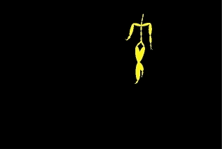
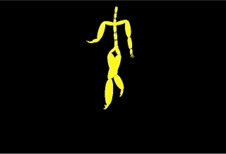
(a) “Walk” sequence.
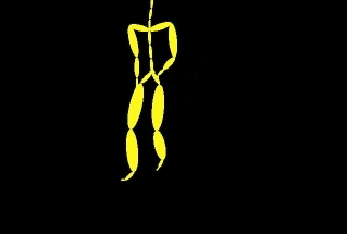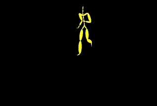
(b) “Run” sequence.

Figure 1: Examples of motion capture sequences from the MoCap dataset, shown with stick figures.

Figure 2: An example of hierarchical clustering of the MoCap dataset, with VHEM-H3M and PPK-SC. Different colors represent different motion classes. Vertical bars represent clusters, with the colors indicating the proportions of the motion classes in a cluster, and the numbers on the x-axes representing the clusters’ indexes. At Level 1 there are $56$ clusters, one for each motion sequence. At Levels $2$, $3$ and $4$ there are $8$, $4$ and $2$ HMM clusters, respectively. For VHEM almost all clusters at Level 2 are populated by examples from a single motion class. The error of VHEM in clustering a portion of “soccer” with “basket” is probably because both actions involve a sequence of movement, shot, and pause. Moving up the hierarchy, the VHEM algorithm clusters similar motions classes together, and at Level 4 creates a dichotomy between “sit” and the other (more dynamic) motion classes. PPK-SC also clusters motion sequences well at Level 2, but incorrectly aggregates “sit” and “soccer”, which have quite different dynamics. At Level 4, the clustering obtained by PPK-SC is harder to interpret than that by VHEM.

In this experiment we test the VHEM algorithm on hierarchical motion clustering from motion capture data, i.e., time series representing human locomotions and actions. To hierarchically cluster a collection of time series, we first model each time series with an HMM and then cluster the HMMs hierarchically. Since each HMM summarizes the appearance and dynamics of the particular motion sequence it represents, the structure encoded in the hierarchy of HMMs directly applies to the original motion sequences. Jebara et al. (2007) uses a similar approach to cluster motion sequences, applying PPK-SC to cluster HMMs. However, they did not extend their study to hierarchies with multiple levels.

5.2.1 Datasets and setup

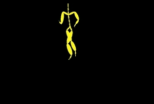
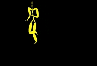
We experiment on two motion capture datasets, the MoCap dataset (http://mocap.cs.cmu.edu/) and the Vicon Physical Action dataset (Theodoridis and Hu, 2007; Frank and Asuncion, 2010). For the MoCap dataset, we use $56$ motion examples spanning $8$ different classes (“jump”, “run”, “jog”, “walk 1”, “walk 2”, “basket”, “soccer”, and “sit”). Each example is a sequence of $123$-dimensional vectors representing the $(x,y,z)$-coordinates of $41$ body markers tracked spatially through time. Figure 1 illustrates some typical examples. We built a hierarchy of $h=4$ levels. The first level (Level 1) was formed by the $K_{1}=56$ HMMs learned from each individual motion example (with $S=4$ hidden states, and $M=2$ components for each GMM emission). The next three levels contain $K_{2}=8$, $K_{3}=4$ and $K_{4}=2$ HMMs. We perform the hierarchical clustering with VHEM-H3M, PPK-SC, EM-H3M, SHEM-H3M ($N\in\{560,2800\}$ and $\tau=10$), and HEM-DTM (state dimension of $7$). The experiments were repeated $10$ times for each clustering method, using different random initializations of the algorithms.

The Vicon Physical Action dataset is a collection of $200$ motion sequences. Each sequence consists of a time series of $27$-dimensional vectors representing the $(x,y,z)$-coordinates of $9$ body markers captured using the Vicon 3D tracker. The dataset includes $10$ normal and $10$ aggressive activities, performed by each of $10$ human subjects a single time. We build a hierarchy of $h=5$ levels, starting with $K_{1}=200$ HMMs (with $S=4$ hidden states and $M=2$ components for each GMM emission) at the first level (i.e., one for each motion sequence), and using $K_{2}=20$, $K_{3}=8$, $K_{4}=4$, and $K_{5}=2$ for the next four levels. The experiment was repeated $5$ times with VHEM-H3M and PPK-SC, using different random initializations of the algorithms.

In similar experiments where we varied the number of levels $h$ of the hierarchy and the number of clusters at each level, we noted similar relative performances of the various clustering algorithms, on both datasets.

5.2.2 Results on the MoCap dataset

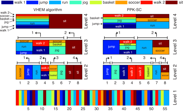
An example of hierarchical clustering of the MoCap dataset with VHEM-H3M is illustrated in Figure 2 (left). In the first level, each vertical bar represents a motion sequence, with different colors indicating different ground-truth classes. In the second level, the $K_{2}=8$ HMM clusters are shown with vertical bars, with the colors indicating the proportions of the motion classes in the cluster. Almost all clusters are populated by examples from a single motion class (e.g., “run”, “jog”, “jump”), which demonstrates that VHEM can group similar motions together. We note an error of VHEM in clustering a portion of the “soccer” examples with “basket”. This is probably caused by the similar dynamics of these actions, which both consist of a sequence of movement, shot, and pause. Moving up the hierarchy, the VHEM algorithm clusters similar motion classes together (as indicated by the arrows), for example “walk 1” and “walk 2” are clustered together at Level 2, and at the highest level (Level 4) it creates a dichotomy between “sit” and the rest of the motion classes. This is a desirable behavior as the kinetics of the “sit” sequences (which in the MoCap dataset correspond to starting in a standing position, sitting on a stool, and returning to a standing position) are considerably different from the rest. On the right of Figure 2, the same experiment is repeated with PPK-SC. PPK-SC clusters motion sequences properly, but incorrectly aggregates “sit” and “soccer” at Level 2, even though they have quite different dynamics. Furthermore, the highest level (Level 4) of the hierarchical clustering produced by PPK-SC is harder to interpret than that of VHEM.

Table 2: Hierarchical clustering of the MoCap dataset using VHEM-H3M, PPK-SC, SHEM-H3M, EM-H3M and HEM-DTM. The number in brackets after SHEM-H3M represents the number of real samples used. We computed Rand-index, data log-likelihood and cluster compactness at each level of the hierarchy, and registered the time (in seconds) to learn the hierarchical structure. Differences in Rand-index at Levels 2, 3, and 4 are statistically significant based on a paired t-test with confidence $95\%$.

	Rand-index			log-likelihood ($\times 10^{6}$)			PPK cluster-compactness			time (s)
Level	2	3	4	2	3	4	2	3	4
VHEM-H3M	0.937	0.811	0.518	-5.361	-5.682	-5.866	0.0075	0.0068	0.0061	30.97
PPK-SC	0.956	0.740	0.393	-5.399	-5.845	-6.068	0.0082	0.0021	0.0008	37.69
SHEM-H3M (560)	0.714	0.359	0.234	-13.632	-69.746	-275.650	0.0062	0.0034	0.0031	843.89
SHEM-H3M (2800)	0.782	0.685	0.480	-14.645	-30.086	-52.227	0.0050	0.0036	0.0030	3849.72
EM-H3M	0.831	0.430	0.340	-5.713	-202.55	-168.90	0.0099	0.0060	0.0056	667.97
HEM-DTM	0.897	0.661	0.412	-7.125	-8.163	-8.532	-	-	-	121.32

Table 2 presents a quantitative comparison between PPK-SC and VHEM-H3M at each level of the hierarchy. While VHEM-H3M has lower Rand-index than PPK-SC at Level 2 ($0.937$ vs. $0.956$), VHEM-H3M has higher Rand-index at Level 3 ($0.811$ vs. $0.740$) and Level 4 ($0.518$ vs. $0.393$). In terms of PPK cluster-compactness, we observe similar results. In particular, VHEM-H3M has higher PPK cluster-compactness than PPK-SC at Level 3 and 4. Overall, keeping in mind that PPK-SC is explicitly driven by PPK-similarity, while the VHEM-H3M algorithm is not, these results can be considered as strongly in favor of VHEM-H3M (over PPK-SC). In addition, the data log-likelihood for VHEM-H3M is higher than that for PPK-SC at each level of the hierarchy. This suggests that the novel HMM cluster centers learned by VHEM-H3M fit the motion capture data better than the spectral cluster centers. This conclusion is further supported by the results of the density estimation experiments in Sections 6.1 and 6.2. Note that the higher up in the hierarchy, the more clearly this effect is manifested.

Comparing to other methods (also in Table 2), EM-H3M generally has lower Rand-index than VHEM-H3M and PPK-SC (consistent with the results in (Jebara et al., 2007)). While EM-H3M directly clusters the original motion sequences, both VHEM-H3M and PPK-SC implicitly integrate over all possible virtual variations of the original motion sequences (according to the intermediate HMM models), which results in more robust clustering procedures. In addition, EM-H3M has considerably longer running times than VHEM-H3M and PPK-SC (i.e., roughly $20$ times longer) since it needs to evaluate the likelihood of all training sequences at each iteration, at all levels.

The results in Table 2 favor VHEM-H3M over SHEM-H3M, and empirically validate the variational approximation that VHEM uses for learning. For example, when using $N=2800$ samples, running SHEM-H3M takes over two orders of magnitude more time than VHEM-H3M, but still does not achieve performance competitive with VHEM-H3M. With an efficient closed-form expression for averaging over all possible virtual samples, VHEM approximates the sufficient statistics of a virtually unlimited number of observation sequences, without the need of using real samples. This has an additional regularization effect that improves the robustness of the learned HMM cluster centers. In contrast, SHEM-H3M uses real samples, and requires a large number of them to learn accurate models, which results in significantly longer running times.

Finally, in Table 2, we also report hierarchical clustering performance for HEM-DTM. VHEM-H3M consistently outperforms HEM-DTM, both in terms of Rand-index and data log-likelihood. Since both VHEM-H3M and HEM-DTM are based on the hierarchical EM algorithm for learning the clustering, this indicates that HMM-based clustering models are more appropriate than DT-based models for the human MoCap data. Note that, while PPK-SC is also HMM-based, it has a lower Rand-index than HEM-DTM at Level 4. This further suggests that PPK-SC does not optimally cluster the HMMs.

Table 3: Hierarchical clustering of the Vicon Physical Action dataset using VHEM-H3M and PPK-SC. Performance is measured in terms of Rand-index, data log-likelihood and PPK cluster-compactness at each level. Differences in Rand-index at Levels 2, 4 and 5 are statistically significant based on a paired t-test with confidence $95\%$. The test failed at Level 3.

	Rand-index				log-likelihood ($\times 10^{6}$)				PPK cluster-compactness
Level	2	3	4	5	2	3	4	5	2	3	4	5
VHEM-H3M	0.909	0.805	0.610	0.244	-1.494	-3.820	-5.087	-6.172	0.224	0.059	0.020	0.005
PPK-SC	0.900	0.807	0.452	0.092	-3.857	-5.594	-6.163	-6.643	0.324	0.081	0.026	0.008

5.2.3 Results on the Vicon Physical Action dataset

Table 3 presents results using VHEM-H3M and PPK-SC to cluster the Vicon Physical Action dataset. While the two algorithms performs similarly in terms of Rand-index at lower levels of the hierarchy (i.e., Level 2 and Level 3), at higher levels (i.e., Level 4 and Level 5) VHEM-H3M outperforms PPK-SC. In addition, VHEM-H3M registers higher data log-likelihood than PPK-SC at each level of the hierarchy. This, again, suggests that by learning new cluster centers, the VHEM-H3M algorithm retains more information on the clusters’ structure than PPK-SC. Finally, compared to VHEM-H3M, PPK-SC produces clusters that are more compact in terms of PPK similarity. However, this does not necessarily imply a better agreement with the ground truth clustering, as evinced by the Rand-index metrics.

5.3 Clustering synthetic data

In this experiment, we compare VHEM-H3M and PPK-SC on clustering a synthetic dataset of HMMs.

5.3.1 Dataset and setup

The synthetic dataset of HMMs is generated as follows. Given a set of $C$ HMMs $\{{\cal M}^{(c)}\}_{c=1}^{C}$, for each HMM we synthesize a set of $K$ “noisy” versions of the original HMM. Each “noisy” HMM $\tilde{\cal M}^{(c)}_{k}$ ($k=1,\dots K$) is synthesized by generating a random sequence $y_{1:T}$ of length $T$ from ${\cal M}^{(c)}$, corrupting it with Gaussian noise $\sim{\cal N}(0,\sigma_{n}^{2}\mathrm{I}_{d})$, and estimating the parameters of $\tilde{\cal M}^{(c)}_{k}$ on the corrupted version of $y_{1:T}$. Note that this procedure adds noise in the observation space. The number of noisy versions (of each given HMM), $K$, and the noise variance, $\sigma_{n}^{2}$, will be varied during the experiments.

The collection of original HMMs was created as follows. Their number was always set to $C=4$, the number of hidden states of the HMMs to $S=3$, the emission distributions to be single, one-dimensional Gaussians (i.e., GMMs with $M=1$ component), and the length of the sequences to $T=100$. For all original HMMs ${\cal M}^{(c)}$, the initial state probability and state transition matrix were fixed as

$$\pi^{(c)}=\left[\begin{array}[]{c}1/3\\ 1/3\\ 1/3\\ \end{array}\right],\quad A^{(c)}=\left[\begin{array}[]{ccc}0.8&0.1&0.1\\ 0.2&0.8&0\\ 0&0.2&0.8\\ \end{array}\right],\forall c.$$ (67)

We consider two settings of the emission distributions. In the first setting, experiment (a), the HMMs ${\cal M}^{(c)}$ only differ in the means of the emission distributions,

$$\begin{split}&\left\{\begin{array}[]{c}\mu^{(1)}_{1}=1\\ \mu^{(1)}_{2}=2\\ \mu^{(1)}_{3}=3\\ \end{array}\right.,\left\{\begin{array}[]{c}\mu^{(2)}_{1}=3\\ \mu^{(2)}_{2}=2\\ \mu^{(2)}_{3}=1\\ \end{array}\right.,\left\{\begin{array}[]{c}\mu^{(3)}_{1}=1\\ \mu^{(3)}_{2}=2\\ \mu^{(3)}_{3}=2\\ \end{array}\right.,\left\{\begin{array}[]{c}\mu^{(4)}_{1}=1\\ \mu^{(4)}_{2}=3\\ \mu^{(4)}_{3}=3\\ \end{array}\right.,\quad{\sigma^{(c)}_{\rho}}^{2}=0.5,\quad\forall\rho,c.\end{split}$$ (68)

In the second setting, experiment (b), the HMMs differ in the variances of the emission distributions,

$$\begin{split}&\left\{\begin{array}[]{c}\mu^{(c)}_{1}=1\\ \mu^{(c)}_{2}=2\\ \mu^{(c)}_{3}=3\\ \end{array}\right.,\forall c,\quad{\sigma^{(1)}_{\rho}}^{2}=0.5,\quad{\sigma^{(2)}_{\rho}}^{2}=0.1,\quad{\sigma^{(3)}_{\rho}}^{2}=1,\quad{\sigma^{(4)}_{\rho}}^{2}=0.05,\quad\forall\rho.\end{split}$$ (69)

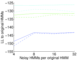
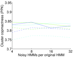
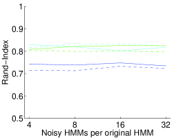
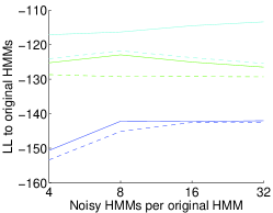
The VHEM-H3M and PPK-SC algorithms are used to cluster the synthesized HMMs, $\{\{\tilde{\cal M}^{(c)}_{k}\}_{k=1}^{K}\}_{c=1}^{C}$, into $C$ groups, and the quality of the resulting clusterings is measured with the Rand-index, PPK cluster-compactness, and the expected log-likelihood of the discovered cluster centers with respect to the original HMMs. The expected log-likelihood was computed using the lower bound, as in (19), with each of the original HMMs assigned to the most likely HMM cluster center. The results are averages over $10$ trials.

5.3.2 Results

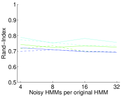
Figure 3 reports the performance metrics when varying the number $K\in\{2,4,8,16,32\}$ of noisy versions of each of the original HMMs, and the noise variance $\sigma_{n}^{2}\in\{0.1,0.5,1\}$, for the two experimental settings.

Experiment (a): different emission means.
Experiment (b): different emission variances.

Figure 3: Results on clustering synthetic data with VHEM-H3M and PPK-SC. Performance is measured in terms of Rand-index, expected log-likelihood and PPK cluster-compactness.

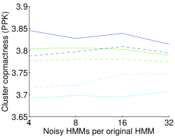For the majority of settings of $K$ and $\sigma_{n}^{2}$, the clustering produced by VHEM-H3M is superior to the one produced by PPK-SC, for each of the considered metrics (i.e., in the plots, solid lines are usually above dashed lines of the same color). The only exception is in experiment (b) where, for low noise variance (i.e., $\sigma_{n}^{2}=0.1$) PPK-SC is the best in terms of Rand-index and cluster compactness. It is interesting to note that the gap in performance between VHEM-H3M and PPK-SC is generally larger at low values of $K$. We believe this is because, when only a limited number of input HMMs is available, PPK-SC produces an embedding of lower quality. This does not affect VHEM-H3M, since it clusters in HMM distribution space and does not use an embedding.

These results suggest that, by clustering HMMs directly in distribution space, VHEM-H3M is generally more robust than PPK-SC, the performance of which instead depends on the quality of the underlying embedding.

6 Density estimation experiments

In this section, we present an empirical study of VHEM-H3M for density estimation, in automatic annotation and retrieval of music (Section 6.1) and hand-written digits (Section 6.2).

6.1 Music annotation and retrieval

In this experiment, we evaluate VHEM-H3M for estimating annotation models in content-based music auto-tagging. As a generative time-series model, H3Ms allow to account for timbre (i.e., through the GMM emission process) as well as longer term temporal dynamics (i.e., through the HMM hidden state process), when modeling musical signals. Therefore, in music annotation and retrieval applications, H3Ms are expected to prove more effective than existing models that do not explicitly account for temporal information (Turnbull et al., 2008; Mandel and Ellis, 2008; Eck et al., 2008; Hoffman et al., 2009).

6.1.1 Music dataset

We consider the CAL500 collection from (Turnbull et al., 2008), which consists of 502 songs and provides binary annotations with respect to a vocabulary ${\cal V}$ of 149 tags, ranging from genre and instrumentation, to mood and usage. To represent the acoustic content of a song we extract a time series of audio features ${\cal Y}=\{y_{1},\dots,y_{|{\cal Y}|}\}$, by computing the first 13 Mel frequency cepstral coefficients (MFCCs) (Rabiner and Juang, 1993) over half-overlapping windows of $46$ms of audio signal, augmented with first and second instantaneous derivatives. The song is then represented as a collection of audio fragments, which are sequences of $T=125$ audio features (approximately 6 seconds of audio), using a dense sampling with $80\%$ overlap.

6.1.2 Music annotation models

Automatic music tagging is formulated as a supervised multi-label problem (Carneiro et al., 2007), where each class is a tag from ${\cal V}$. We approach this problem by modeling the audio content for each tag with a H3M probability distribution. I.e., for each tag, we estimate an H3M over the audio fragments of the songs in the database that have been associated with that tag, using the hierarchical estimation procedure based on VHEM-H3M. More specifically, the database is first processed at the song level, using the EM algorithm to learn a H3M with $K^{(s)}=6$ components for each song from its audio fragments. Then, for each tag, the song-level H3Ms labeled with that tag are pooled together to form a large H3M, and the VHEM-H3M algorithm is used to reduce this to a final H3M tag-model with $K=3$ components ($\tau=10$ and $N=N_{v}N_{t}K^{(s)}$, where $N_{v}=1000$ and $N_{t}$ is the number of training songs for the particular tag).

Given the tag-level models, a song can be represented as a vector of posterior probabilities of each tag (a semantic multinomial, SMN), by extracting features from the song, computing the likelihood of the features under each tag-level model, and applying Bayes’ rule. A test song is annotated with the top-ranking tags in its SMN. To retrieve songs given a tag query, a collection of songs is ranked by the tag’s probability in their SMNs.

We compare VHEM-H3M with three alternative algorithms for estimating the H3M tag models: PPK-SC, PPK-SC-hybrid, and EM-H3M. For all three alternatives, we use the same number of mixture components in the tag models ($K=3$). For the two PPK-SC methods, we leverage the work of Jebara et al. (2007) to learn H3M tag models, and use it in place of the VHEM-H3M algorithm in the second stage of the hierarchical estimation procedure. We found that it was necessary to implement the PPK-SC approaches with song-level H3Ms with only $K^{(s)}=1$ component (i.e., a single HMM), since the computational cost for constructing the initial embedding scales poorly with the number of input HMMs. PPK-SC first applies spectral clustering to the song-level HMMs and then selects as the cluster centers the HMMs that map closest to the spectral cluster centers in the spectral embedding. PPK-SC-hybrid is a hybrid method combining PPK-SC for clustering, and VHEM-H3M for estimating the cluster centers. Specifically, after spectral clustering, HMM cluster centers are estimated by applying VHEM-H3M (with $K^{(r)}=1$) to the HMMs assigned to each of the resulting clusters. In other words, PPK-SC and PPK-SC-hybrid use spectral clustering to summarize a collection of song-level HMMs with a few HMM centers, forming a H3M tag model. The mixture weight of each HMM component (in the H3M tag model) is set proportional to the number of HMMs assigned to that cluster.

For EM-H3M, the H3M tag models were estimated directly from the audio fragments from the relevant songs using the EM-H3M algorithm. Empirically, we found that, due to its runtime and RAM requirements, for EM-H3M we must use non-overlapping audio-fragments and evenly subsample by $73\%$ on average, resulting in $14.5\%$ of the sequences used by VHEM-H3M. Note that, however, EM-H3M is still using $73\%$ of the actual song data (just with non-overlapping sequences). We believe this to be a reasonable comparison between EM and VHEM, as both methods use roughly similar resources (the sub-sampled EM is still $3$ times slower, as reported in Table 4). Based on our projections, running EM over densely sampled song data would require roughly $9000$ hours of CPU time (e.g., more than $5$ weeks when parallelizing the algorithm over $10$ processors), as opposed to 630 hours for VHEM-H3M. This would be extremely cpu-intensive given the computational limits of our cluster. The VHEM algorithm, on the other hand, can learn from considerable amounts of data while still maintaining low runtime and memory requirements.

Finally, we also compare against two state-of-the-art models for music tagging, HEM-DTM (Coviello et al., 2011), which is based on a different time-series model (mixture of dynamic textures), and HEM-GMM (Turnbull et al., 2008), which is a bag-of-features model using GMMs. Both methods use efficient hierarchical estimation based on a HEM algorithm (Chan et al., 2010b; Vasconcelos and Lippman, 1998) to obtain the tag-level models.

6.1.3 Performance metrics

A test song is annotated with the 10 most likely tags, and annotation performance is measured with the per-tag precision (P), recall (R), and F-score (F), averaged over all tags. If $|w_{H}|$ is the number of test songs that have the tag $w$ in their ground truth annotations, $|w_{A}|$ is the number of times an annotation system uses $w$ when automatically tagging a song, and $|w_{C}|$ is the number of times $w$ is correctly used, then precision, recall and F-score for the tag $w$ are defined as:

$$\mbox{P}=\frac{|w_{C}|}{|w_{A}|},\,\,\,\mbox{R}=\frac{|w_{C}|}{|w_{H}|},\,\,\,\mbox{F}=2\left((\mbox{P})^{-1}+(\mbox{R})^{-1}\right)^{-1}.$$ (70)

Retrieval is measured by computing per-tag mean average precision (MAP) and precision at the first $k$ retrieved songs (P@$k$), for $k\in\{5,10,15\}$. The P@$k$ is the fraction of true positives in the top-$k$ of the ranking. MAP averages the precision at each point in the ranking where a song is correctly retrieved. All reported metrics are averages over the 97 tags that have at least 30 examples in CAL500 (11 genre, 14 instrument, 25 acoustic quality, 6 vocal characteristics, 35 emotion and 6 usage tags), and are the result of 5-fold cross-validation.

Finally, we also record the total time (in hours) to learn the $97$ tag-level H3Ms on the 5 splits of the data. For hierarchical estimation methods (VHEM-H3M and the PPK-SC approaches), this also includes the time to learn the song-level H3Ms.

Table 4: Annotation and retrieval performance on CAL500, for VHEM-H3M, PPK-SC, PPK-SC-hybrid, EM-H3M, HEM-DTM (Coviello et al., 2011) and HEM-GMM (Turnbull et al., 2008).

	annotation			retrieval
	P	R	F	MAP	P@5	P@10	P@15	time ($h$)
VHEM-H3M	0.446	0.211	0.260	0.440	0.474	0.451	0.435	629.5
PPK-SC	0.299	0.159	0.151	0.347	0.358	0.340	0.329	974.0
PPK-SC-hybrid	0.407	0.200	0.221	0.415	0.439	0.421	0.407	991.7
EM-H3M	0.415	0.214	0.248	0.423	0.440	0.422	0.407	1860.4
HEM-DTM	0.431	0.202	0.252	0.439	0.479	0.454	0.428	-
HEM-GMM	0.374	0.205	0.213	0.417	0.441	0.425	0.416	-

6.1.4 Results

In Table 4 we report the performance of the various algorithms for both annotation and retrieval on the CAL500 dataset. Looking at the overall runtime, VHEM-H3M is the most efficient algorithm for estimating H3M distributions from music data, as it requires only $34\%$ of the runtime of EM-H3M, and $65\%$ of the runtime of PPK-SC. The VHEM-H3M algorithm capitalizes on the first stage of song-level H3M estimation (about one third of the total time) by efficiently and effectively using the song-level H3Ms to learn the final tag models. Note that the runtime of PPK-SC corresponds to setting $K^{(s)}=1$. When we set $K^{(s)}=2$, we registered a running time four times longer, with no significant improvement in performance.

The gain in computational efficiency does not negatively affect the quality of the corresponding models. On the contrary, VHEM-H3M achieves better performance than EM-H3M, strongly improving the top of the ranked lists, as evinced by the higher P@$k$ scores. Relative to EM-H3M, VHEM-H3M has the benefit of regularization, and during learning can efficiently leverage all the music data condensed in the song H3Ms. VHEM-H3M also outperforms both PPK-SC approaches on all metrics. PPK-SC discards considerable information on the clusters’ structure by selecting one of the original HMMs to approximate each cluster. This significantly affects the accuracy of the resulting annotation models. VHEM-H3M, on the other hand, generates novel HMM cluster centers to summarize the clusters. This allows to retain more accurate information in the final annotation models.

PPK-SC-hybrid achieves considerable improvements relative to standard PPK-SC, at relatively low additional computational costs. This further demonstrates that the VHEM-H3M algorithm can effectively summarize in a smaller model the information contained in several HMMs. In addition, we observe that VHEM-H3M still outperforms PPK-SC-hybrid, suggesting that the former produces more accurate cluster centers and density estimates. In fact, VHEM-H3M couples clustering and learning HMM cluster centers, and is entirely based on maximum likelihood for estimating the H3M annotation models. PPK-SC-hybrid, on the contrary, separates clustering and parameter estimation, and optimizes them against two different metrics (i.e., PPK similarity and expected log-likelihood, respectively). As a consequence, the two phases may be mismatched, and the centers learned with VHEM may not be the best representatives of the clusters according to PPK affinity.

Finally, VHEM-H3M compares favorably to the auto-taggers based on other generative models. First, VHEM-H3M outperforms HEM-GMM, which does not model temporal information in the audio signal, on all metrics. Second, the performances of VHEM-H3M and HEM-DTM (a continuous-state temporal model) are not statistically different based on a paired t-test with $95\%$ confidence, except for annotation precision where VHEM-H3M scores significantly higher. Since HEM-DTM is based on linear dynamic systems (a continuous-state model), it can model stationary time-series in a linear subspace. In contrast, VHEM-H3M uses HMMs with discrete states and GMM emissions, and can hence better adapt to non-stationary time-series on a non-linear manifold. This difference is illustrated in the experiments: VHEM-H3M outperforms HEM-DTM on the human MoCap data (see Table 2), which has non-linear dynamics, while the two perform similarly on the music data (see Table 4), where audio features are often stationary over short time frames.

6.2 On-line hand-writing data classification and retrieval

In this experiment, we investigate the performance of the VHEM-H3M algorithm in estimating class-conditional H3M distributions for automatic classification and retrieval of on-line hand-writing data.

6.2.1 Dataset

We consider the Character Trajectories Data Set (Frank and Asuncion, 2010), which is a collection of $2858$ examples of characters from the same writer, originally compiled to study handwriting motion primitives (Williams et al., 2006). Each example is the trajectory of one of the $20$ different characters that correspond to a single pen-down segment. The data was captured from a WACOM tablet at 200 Hz, and consists of $(x,y)$-coordinates and pen tip force. The data has been numerically differentiated and Gaussian smoothed (Williams et al., 2006). Half of the data is used for training, with the other half held out for testing.

6.2.2 Classification models and setup

From the hand-writing examples in the training set, we estimate a series of class-conditional H3M distributions, one for each character, using hierarchical estimation with the VHEM-H3M algorithm. First, for each character, we partition all the relevant training data into groups of $3$ sequences, and learn a HMM (with $S=4$ states and $M=1$ component for the GMM emissions) from each group using the Baum-Welch algorithm. Next, we estimate the class-conditional distribution (classification model) for each character by aggregating all the relevant HMMs and summarizing them into a H3M with $K=4$ components using the VHEM-H3M algorithm ($\tau=10$ and $N=N_{v}N_{c}$, where $N_{v}=10$, and $N_{c}$ is the number of intermediate models for that character). Using the character-level H3Ms and Bayes’ rule, for each hand-writing example in the test set we compute the posterior probabilities of all of the 20 characters. Each example is classified as the character with largest posterior probability. For retrieval given a query character, examples in the test set are ranked by the character’s posterior probability.

We repeated the same experiment using PPK-SC or SHEM-H3M ($\tau=10$, $N=1000$) to estimate the classification models from the intermediate HMMs. Finally, we considered the EM-H3M algorithm, which directly uses the training sequences to learn the class-conditional H3M ($K=4$).

Since VHEM-H3M, SHEM-H3M and EM-H3M are iterative algorithms, we studied them when varying the stopping criterion. In particular, the algorithms were terminated when the relative variation in the value of the objective function between two consecutive iterations was lower than a threshold $\Delta LL$, which we varied in $\{10^{-2},10^{-3},10^{-4},10^{-5}\}$.

Finally, we measure classification and retrieval performance on the test set using the classification accuracy, and the average per-tag P@$3$ and P@$5$. We also report the total training time, which includes the time used to learn the intermediate HMMs. The experiments consisted of 5 trials with different random initializations of the algorithms.

6.2.3 Results

Table 5: Classification and retrieval performance, and training time on the Character Trajectories Data Set, for VHEM-H3M, PPK-SC, SHEM-H3M, and EM-H3M.

	stop	retrieval		classification
	$\Delta LL$	P@3	P@5	Accuracy	total time (s)
VHEM-H3M	$10^{-2}$	0.750	0.750	0.618	1838.34
	$10^{-3}$	0.717	0.750	0.619	1967.55
	$10^{-4}$	0.733	0.790	0.648	2210.77
	$10^{-5}$	0.750	0.820	0.651	2310.93
SHEM-H3M	$10^{-2}$	0.417	0.440	0.530	13089.32
	$10^{-3}$	0.683	0.680	0.664	23203.44
	$10^{-4}$	0.700	0.750	0.689	35752.20
	$10^{-5}$	0.700	0.750	0.690	50094.36
EM-H3M	$10^{-2}$	0.583	0.610	0.646	6118.53
	$10^{-3}$	0.617	0.650	0.674	7318.56
	$10^{-4}$	0.650	0.710	0.707	9655.08
	$10^{-5}$	0.517	0.560	0.635	10957.38
PPK-SC	-	0.600	0.700	0.646	1463.54

Table 5 lists the classification and retrieval performance on the test set for the various methods. Consistent with the experiments on music annotation and retrieval (Section 6.1), VHEM-H3M performs better than PPK-SC on all metrics. By learning novel HMM cluster centers, VHEM-H3M estimates H3M distributions that are representative of all the relevant intermediate HMMs, and hence of all the relevant training sequences. While EM-H3M is the best in classification (at the price of longer training times), VHEM-H3M performs better in retrieval, as evinced by the P@$3$ and P@$5$ scores. In terms of training time, VHEM-H3M and PPK-SC are about $5$ times faster than EM-H3M. In particular, PPK-SC is the fastest algorithm, since the small number of input HMMs (i.e., on average $23$ per character) allows to build the spectral clustering embedding efficiently.

The version of HEM based on actual sampling (SHEM-H3M) performs better than VHEM-H3M in classification, but VHEM-H3M has higher retrieval scores. However, the training time for SHEM-H3M is approximately $15$ times longer than for VHEM-H3M. In order to reliably estimate the reduced models, the SHEM-H3M algorithm requires generating a large number of samples, and computing their likelihood at each iteration. In contrast, the VHEM-H3M algorithm efficiently approximates the sufficient statistics of a virtually unlimited number of samples, without the need of using real samples.

It is also interesting to note that EM-H3M appears to suffer from overfitting of the training set, as suggested by the overall drop in performance when the stopping criterion changes from $\Delta LL=10^{-4}$ to $\Delta LL=10^{-5}$. In contrast, both VHEM-H3M and SHEM-H3M consistently improve on all metrics as the algorithm converges (again looking at $\Delta LL\in\{10^{-4},10^{-5}\}$). These results suggest that the regularization effect of hierarchical estimation, which is based on averaging over more samples (either virtual or actual), can positively impact the generalization of the learned models.

Finally, we elaborate on how these results compare to the experiments on music annotation and retrieval (in Section 6.1). First, in the Character Trajectory Data Set the number of training sequences associated with each class (i.e, each character) is small compared to the CAL500 dataset. As a result, the EM-H3M algorithm is able to process all the data, and achieve good classification performance. However, EM-H3M still needs to evaluate the likelihood of all the original sequences at each iteration. This leads to slower iterations, and results in a total training time about $5$ times longer than that of VHEM-H3M (see Table 5). Second, the Character Trajectory data is more “controlled” than the CAL500 data, since each class corresponds to a single character, and all the examples are from the same writer. As a consequence, there is less variation in the intermediate HMMs (i.e., they are clustered more closely), and several of them may summarize the cluster well, providing good candidate cluster centers for PPK-SC. In conclusion, PPK-SC faces only a limited loss of information when selecting one of the initial HMMs to represent each cluster, and achieves reasonable performances.

6.3 Robustness of VHEM-H3M to number and length of virtual samples

Table 6: Annotation and retrieval performance on CAL500 for VHEM-H3M when varying the virtual sample parameters $N_{v}$ and $\tau$.

	$N_{v}=1000$				$\tau=10$
	$\tau=2$	$\tau=5$	$\tau=10$	$\tau=20$	$N_{v}=1$	$N_{v}=10$	$N_{v}=100$	$N_{v}=1000$
P@5	0.4656	0.4718	0.4738	0.4734	0.4775	0.4689	0.4689	0.4738
P@10	0.4437	0.4487	0.4507	0.4478	0.4534	0.4491	0.4466	0.4507
P@15	0.4236	0.4309	0.4346	0.4327	0.4313	0.4307	0.4242	0.4346

The generation of virtual samples in VHEM-H3M is controlled by two parameters: the number of virtual sequences ($N$), and their length ($\tau$). In this section, we investigate the impact of these parameters on annotation and retrieval performance on CAL500. For a given tag $t$, we set $N=N_{v}N_{t}K^{(s)}$, where $N_{v}$ is a constant, $N_{t}$ the number of training songs for the tag, and $K^{(s)}$ the number of mixture components for each song-level H3M. Starting with $(N_{v},\tau)=(1000,10)$, each parameter is varied while keeping the other one fixed, and annotation and retrieval performance on the CAL500 dataset are calculated, as described in Section 6.1.

Table 6 presents the results, for $\tau\in\{2,5,10,20\}$ and $N_{v}\in\{1,10,100,1000\}$. The performances when varying $\tau$ are close on all metrics. For example, average P@5, P@10 and P@15 vary in small ranges ($0.0082$, $0.0070$ and $0.0110$, respectively). Similarly, varying the number of virtual sequences $N_{v}$ has a limited impact on performance as well. This demonstrates that VHEM-H3M is fairly robust to the choice of these parameters.

Finally, we tested VHEM-H3M for music annotation and retrieval on CAL500, using virtual sequences of the same length as the audio fragments used at the song level, i.e., $\tau=T=125$. Compared to $\tau=10$ (the setting used in earlier experiments), we registered an $84\%$ increase in total running time, with no corresponding improvement in performance. Thus, in our experimental setting, making the virtual sequences relatively short positively impacts the running time, without reducing the quality of the learned models.

7 Conclusion

In this paper, we presented a variational HEM (VHEM) algorithm for clustering HMMs with respect to their probability distributions, while generating a novel HMM center to represent each cluster. Experimental results demonstrate the efficacy of the algorithm on various clustering, annotation, and retrieval problems involving time-series data, showing improvement over current methods. In particular, using a two-stage, hierarchical estimation procedure — learn H3Ms on many smaller subsets of the data, and summarize them in a more compact H3M model of the data — the VHEM-H3M algorithm estimates annotation models from data more efficiently than standard EM and also improves model robustness through better regularization. Specifically, averaging over all possible virtual samples prevents over-fitting, which can improve the generalization of the learned models. Moreover, using relatively short virtual sequences positively impacts the running time of the algorithm, without negatively affecting its performance on practical applications. In addition, we have noted that the VHEM-H3M algorithm is robust to the choice of the number and length of virtual samples.

In our experiments, we have implemented the first stage of the hierarchical estimation procedure by partitioning data in non-overlapping subsets (and learning an intermediate H3M on each subset). In particular, partitioning the CAL500 data at the song level had a practical advantage. Since individual songs in CAL500 are relevant to several tags, the estimation of the song H3Ms can be executed one single time for each song in the database, and re-used in the VHEM estimation of all the associated tag models. This has a positive impact on computational efficiency. Depending on the particular application, however, a slightly different implementation of this first stage (of the hierarchical estimation procedure) may be better suited. For example, when estimating a H3M from a very large amount of training data, one could use a procedure that does not necessarily cover all data, inspired by Kleiner et al. (2011). If $n$ is the size of the training data, first estimate $B>1$ intermediate H3Ms on as many (possibly overlapping) “little” bootstrap subsamples of the data, each of size $b<n$. Then summarize all the intermediate H3Ms into a final H3M using the VHEM-H3M algorithm.

In future work we plan to extend VHEM-H3M to the case where all HMMs share a large GMM universal background model for the emission distributions (with each HMM state having a different set of weights for the Gaussian components), which is commonly used in speech (Huang and Jack, 1989; Bellegarda and Nahamoo, 1990; Rabiner and Juang, 1993). This would allow for faster training (moving the complexity to estimating the noise background model) and would require a faster implementation of the inference (e.g., using a strategy similar to (Coviello et al., 2012b)). In addition, we plan to derive a HEM algorithm for HMMs with discrete emission distributions, and compare its performance to the work presented here and to the extension with the large GMM background model.

Acknowledgments

E.C. thanks Yingbo Song for providing the code of (Jebara et al., 2007) and assistance with the experiments on motion clustering. The authors acknowledge support from Google, Inc. E.C. and G.R.G.L. also wish to acknowledge support from Qualcomm, Inc., Yahoo! Inc., the Hellman Fellowship Program, and the National Science Foundation (grants CCF-0830535 and IIS-1054960). A.B.C. was supported by the Research Grants Council of the Hong Kong Special Administrative Region, China (CityU 110610). G.R.G.L. acknowledges support from the Alfred P. Sloan Foundation. This research was supported in part by the UCSD FWGrid Project, NSF Research Infrastructure Grant Number EIA-0303622.

Appendix A. Derivation of the E-step

The maximization of (42) with respect to $\phi^{i,j}_{t}(\rho_{t}|\rho_{t-1},\beta_{t})$ and $\phi^{i,j}_{1}(\rho_{1}|\beta_{1})$ is carried out independently for each pair $(i,j)$, and follow (Hershey et al., 2008). In particular it uses a backward recursion, starting with ${\cal L}^{i,j}_{\tau+1}(\beta_{t},\rho_{t})=0$, for $t=\tau,\dots,2$,

$$\hat{\phi}^{i,j}_{t}(\rho_{t}|\rho_{t-1},\beta_{t})={} \frac{a^{(r),j}_{\rho_{t-1},\rho_{t}}\exp\left\{{\cal L}_{\text{\tiny GMM}}^{(i,\beta_{t}),(j,\rho_{t})}+{\cal L}^{i,j}_{t+1}(\beta_{t},\rho_{t})\right\}}{\sum_{\rho}^{S}a^{(r),j}_{\rho_{t-1},\rho}\exp\left\{{\cal L}_{\text{\tiny GMM}}^{(i,\beta_{t}),(j,\rho)}+{\cal L}^{i,j}_{t+1}(\beta_{t},\rho)\right\}}$$ (71)

$${\cal L}^{i,j}_{t}(\beta_{t-1},\rho_{t-1})={} \sum_{\beta=1}^{S}a^{(b),i}_{\beta_{t-1},\beta}\log\sum_{\rho=1}^{S}a^{(r),j}_{\rho_{t-1},\rho}\exp\left\{{\cal L}_{\text{\tiny GMM}}^{(i,\beta),(j,\rho)}+{\cal L}^{i,j}_{t+1}(\beta,\rho)\right\},$$ (72)

and terminates with

$$\hat{\phi}^{i,j}_{1}(\rho_{1}|\beta_{1})={} \frac{\pi^{(r),j}_{\rho_{1}}\exp\left\{{\cal L}_{\text{\tiny GMM}}^{(i,\beta_{1}),(j,\rho_{1})}+{\cal L}^{i,j}_{2}(\beta_{1},\rho_{1})\right\}}{\sum_{\rho}^{S}\pi^{(r),j}_{\rho}\exp\left\{{\cal L}_{\text{\tiny GMM}}^{(i,\beta_{1}),(j,\rho)}+{\cal L}^{i,j}_{2}(\beta_{1},\rho)\right\}}$$ (73)

$${\cal L}_{\text{\tiny HMM}}^{i,j}={} \sum_{\beta=1}^{S}\pi^{(b),i}_{\beta}\log\sum_{\rho=1}^{S}\pi^{(r),j}_{\rho}\exp\left\{{\cal L}_{\text{\tiny GMM}}^{(i,\beta),(j,\rho)}+{\cal L}^{i,j}_{2}(\beta,\rho)\right\}$$ (74)

where (74) is the maxima of the terms in (42) in Section 3.3.1.

Appendix B. Derivation of the M-step

The M-steps involves maximizing the lower bound in (33) with respect to ${{\cal M}^{(r)}}$, while holding the variational distributions fixed,

$${{\cal M}^{(r)}}^{*}=\mathop{\mathrm{argmax}}_{{\cal M}^{(r)}}\sum_{i=1}^{K^{(b)}}{\cal L}_{H3M}^{i}.$$ (75)

Substituting (45) and (46) into the objective function of (75),

$${\cal L}({\cal M}^{(r)})=\sum_{i=1}^{K^{(b)}}{\cal L}_{H3M}^{i}$$ (76)

$$=\sum_{i,j}\hat{z}_{ij}\left\{\log\frac{\omega^{(r)}_{j}}{\hat{z}_{ij}}+N_{i}\sum_{\beta_{1:\tau}}\pi_{\beta_{1:\tau}}^{(b),i}\sum_{\rho_{1:\tau}}\hat{\phi}^{i,j}(\rho_{1:\tau}|\beta_{1:\tau})\left[\log\frac{\pi^{(r),j}_{\rho_{1:\tau}}}{\hat{\phi}^{i,j}(\rho_{1:\tau}|\beta_{1:\tau})}+\sum_{t}{\cal L}_{GMM}^{(i,\beta_{t}),(j,\rho_{t})}\right]\right\}$$ (77)

In the following, we detail the update rules for the parameters of the reduced model ${\cal M}^{(r)}$.

HMMs mixture weights

Collecting terms in (77) that only depend on the mixture weights $\{\omega^{(r)}_{j}\}_{j=1}^{K^{(r)}}$, we have

$$\widetilde{{\cal L}}(\{\omega^{(r)}_{j}\})=\sum_{i}\sum_{j}\hat{z}_{ij}\log\omega^{(r)}_{j}=\sum_{j}\left[\sum_{i}\hat{z}_{ij}\right]\log\omega^{(r)}_{j}$$ (78)

Given the constraints $\sum_{j=1}^{K^{(r)}}\omega^{(r)}_{j}=1$ and $\omega^{(r)}_{j}\geq 0$, (78) is maximized using the result in Appendix C.1, which yields the update in (55).

Initial state probabilities

The objective function in (77) factorizes for each HMM ${\cal M}^{(r)}_{j}$, and hence the parameters of each HMM are updated independently. For the $j$-th HMM, we collect terms in (77) that depend on the initial state probabilities $\{\pi^{(r),j}_{\rho}\}_{\rho=1}^{S}$,

$$\widetilde{{\cal L}}_{j}(\{\pi^{(r),j}_{\rho}\}) =\sum_{i}\hat{z}_{ij}N_{i}\sum_{\beta_{1}}\pi_{\beta_{1}}^{(b),i}\sum_{\rho_{1}}\hat{\phi}^{i,j}_{1}(\rho_{1}|\beta_{1})\log\pi^{(r),j}_{\rho_{1}}$$ (79)

$$=\sum_{\rho_{1}}\sum_{i}\hat{z}_{ij}N_{i}\underbrace{\sum_{\beta_{1}}\pi_{\beta_{1}}^{(b),i}\hat{\phi}^{i,j}_{1}(\rho_{1}|\beta_{1})}_{\hat{\nu}^{i,j}_{1}(\rho_{1})}\log\pi^{(r),j}_{\rho_{1}}$$ (80)

$$=\sum_{\rho}\sum_{i}\hat{z}_{ij}N_{i}\hat{\nu}^{i,j}_{1}(\rho)\log\pi^{(r),j}_{\rho}$$ (81)

$$\propto\sum_{\rho}\left[\sum_{i}\hat{z}_{ij}\omega^{(b)}_{i}\hat{\nu}^{i,j}_{1}(\rho)\right]\log\pi^{(r),j}_{\rho},$$ (82)

where in the (81) we have used the summary statistic defined in (48). Considering the constraints $\sum_{\rho=1}^{S}\pi^{(r),j}_{\rho}=1$ and $\pi^{(r),j}_{\rho}\geq 0$, (82) is maximized using the result in Appendix C.1, giving the update formula in (56).

State transition probabilities

Similarly, for each HMM ${\cal M}^{(r)}_{j}$ and previous state $\rho$, we collect terms in (77) that depend on the transition probabilities $\{a^{(r),j}_{\rho,\rho^{\prime}}\}_{\rho^{\prime}=1}^{S}$,

$$\widetilde{{\cal L}}_{j,\rho}(\{a^{(r),j}_{\rho,\rho^{\prime}}\}_{\rho^{\prime}=1}^{S})=\sum_{i}\hat{z}_{ij}N_{i}\sum_{\beta_{1:\tau}}\pi_{\beta_{1:\tau}}^{(b),i}\sum_{\rho_{1:\tau}}\hat{\phi}^{i,j}(\rho_{1:\tau}|\beta_{1:\tau})\log\pi^{(r),j}_{\rho_{1:\tau}}$$ (83)

$$\propto\sum_{i}\hat{z}_{ij}N_{i}\sum_{\beta_{1:\tau}}\left[\pi^{(b),i}_{\beta_{1}}\prod_{t=2}^{\tau}a^{(b),i}_{\beta_{t-1},\beta_{t}}\right]\sum_{\rho_{1:\tau}}\left[\hat{\phi}^{i,j}_{1}(\rho_{1}|\beta_{1})\prod_{t=2}^{\tau}\hat{\phi}^{i,j}_{t}(\rho_{t}|\rho_{t-1},\beta_{t})\right]\left[\sum_{t=2}^{\tau}\log a^{(r),j}_{\rho_{t-1},\rho_{t}}\right]$$ (84)

$$=\sum_{i}\hat{z}_{ij}N_{i}\sum_{\rho_{1}}\sum_{\rho_{2}}\sum_{\beta_{2}}\underbrace{\sum_{\beta_{1}}\underbrace{\pi^{(b),i}_{\beta_{1}}\hat{\phi}^{i,j}_{1}(\rho_{1}|\beta_{1})}_{\nu_{1}^{i,j}(\rho_{1},\beta_{1})}a^{(b),i}_{\beta_{1},\beta_{2}}\hat{\phi}^{i,j}_{2}(\rho_{2}|\rho_{1},\beta_{2})}_{\xi_{2}^{i,j}(\rho_{1},\rho_{2},\beta_{2})}\left[\log a^{(r),j}_{\rho_{1},\rho_{2}}\right.$$ (85)

$$\qquad+\left.\sum_{\beta_{3:\tau}}\sum_{\rho_{3:\tau}}\prod_{t=3}^{\tau}a^{(b),i}_{\beta_{t-1},\beta_{t}}\prod_{t=3}^{\tau}\hat{\phi}^{i,j}_{t}(\rho_{t}|\rho_{t-1},\beta_{t})\sum_{t=3}^{\tau}\log a^{(r),j}_{\rho_{t-1},\rho_{t}}\right]$$ (86)

$$=\sum_{i}\hat{z}_{ij}N_{i}\sum_{\rho_{1}}\sum_{\rho_{2}}\sum_{\beta_{2}}{\xi_{2}^{i,j}(\rho_{1},\rho_{2},\beta_{2})}\log a^{(r),j}_{\rho_{1},\rho_{2}}$$ (87)

$$\quad+\sum_{i}\hat{z}_{ij}N_{i}\sum_{\rho_{2}}\sum_{\rho_{3}}\sum_{\beta_{3}}\underbrace{\sum_{\beta_{2}}\underbrace{\sum_{\rho_{1}}{\xi_{2}^{i,j}(\rho_{1},\rho_{2},\beta_{2})}}_{\nu_{2}^{i,j}(\rho_{2},\beta_{2})}a^{(b),i}_{\beta_{2},\beta_{3}}\hat{\phi}^{i,j}_{3}(\rho_{3}|\rho_{2},\beta_{3})}_{\xi_{3}^{i,j}(\rho_{2},\rho_{3},\beta_{3})}\left[\log a^{(r),j}_{\rho_{2},\rho_{3}}\right.$$ (88)

$$\qquad+\left.\sum_{\beta_{4:\tau}}\sum_{\rho_{4:\tau}}\prod_{t=4}^{\tau}a^{(b),i}_{\beta_{t-1},\beta_{t}}\prod_{t=4}^{\tau}\hat{\phi}^{i,j}_{t}(\rho_{t}|\rho_{t-1},\beta_{t})\sum_{t=4}^{\tau}\log a^{(r),j}_{\rho_{t-1},\rho_{t}}\right]$$ (89)

$$=\dots$$ (90)

$$=\sum_{i}\hat{z}_{ij}N_{i}\sum_{t=2}^{\tau}\sum_{\rho_{t-1}}\sum_{\rho_{t}}\sum_{\beta_{t}}{\xi_{t}^{i,j}(\rho_{t-1},\rho_{t},\beta_{t})}\log a^{(r),j}_{\rho_{t-1},\rho_{t}}$$ (91)

$$\propto\sum_{i}\hat{z}_{ij}N_{i}\sum_{\rho^{\prime}}\underbrace{\sum_{t=2}^{\tau}\sum_{\beta}{\xi_{t}^{i,j}(\rho,\rho^{\prime},\beta)}}_{\hat{\xi}^{i,j}(\rho,\rho^{\prime})}\log a^{(r),j}_{\rho,\rho^{\prime}}$$ (92)

$$\propto\sum_{\rho^{\prime}=1}^{S}\left[\sum_{i}\hat{z}_{ij}\omega^{(b)}_{i}\hat{\xi}^{i,j}(\rho,\rho^{\prime})\right]\log a^{(r),j}_{\rho,\rho^{\prime}}.$$ (93)

Considering the constraints $\sum_{\rho^{\prime}=1}^{S}a^{(r),j}_{\rho,\rho^{\prime}}=1$ and $a^{(r),j}_{\rho,\rho^{\prime}}\geq 0$, (93) is maximized using the result in Appendix C.1, giving the update in (56).

Emission probability density functions

The cost function (77) factors also for each GMM indexed by $(j,\rho,\ell)$. Factoring (77),

$$\widetilde{{\cal L}}({\cal M}^{(r)}_{j,\rho,\ell})=\sum_{i}\hat{z}_{ij}N_{i}\sum_{\beta_{1:\tau}}\pi_{\beta_{1:\tau}}^{(b),i}\sum_{\rho_{1:\tau}}\hat{\phi}^{i,j}(\rho_{1:\tau}|\beta_{1:\tau})\sum_{t}{\cal L}_{GMM}^{(i,\beta_{t}),(j,\rho_{t})}$$ (94)

$$=\sum_{i}\hat{z}_{ij}N_{i}\sum_{\beta_{1:\tau}}\left[\pi_{\beta_{1}}^{(b),i}\prod_{t=2}^{\tau}a_{\beta_{t-1},\beta_{t}}^{(b),i}\right]\sum_{\rho_{1:\tau}}\left[\hat{\phi}_{1}^{i,j}(\rho_{1}|\beta_{1})\prod_{t=2}^{\tau}\hat{\phi}_{t}^{i,j}(\rho_{t}|\rho_{t-1},\beta_{t})\right]\sum_{t}{\cal L}_{GMM}^{(i,\beta_{t}),(j,\rho_{t})}$$ (95)

$$=\sum_{i}\hat{z}_{ij}N_{i}\sum_{\rho_{1}}\sum_{\beta_{1}}\underbrace{\pi_{\beta_{1}}^{(b),i}\hat{\phi}^{i,j}_{1}(\rho_{1}|\beta_{1})}_{\nu^{i,j}_{1}(\rho_{1},\beta_{1})}\left[{\cal L}_{GMM}^{(i,\beta_{1}),(j,\rho_{1})}\dots\right.$$ (96)

$$\qquad\qquad\qquad\qquad\qquad\left.+\sum_{\beta_{2:\tau}}\prod_{t=2}^{\tau}a_{\beta_{t-1},\beta_{t}}^{(b),i}\sum_{\rho_{2:\tau}}\prod_{t=2}^{\tau}\hat{\phi}^{i,j}(\rho_{t}|\rho_{t-1},\beta_{t})\sum_{t=2}^{\tau}{\cal L}_{GMM}^{(i,\beta_{t}),(j,\rho_{t})}\right]$$ (97)

$$=\sum_{i}\hat{z}_{ij}N_{i}\sum_{\rho_{1}}\sum_{\beta_{1}}\nu^{i,j}_{1}(\rho_{1},\beta_{1}){\cal L}_{GMM}^{(i,\beta_{1}),(j,\rho_{1})}$$ (98)

$$\quad+\sum_{i}\hat{z}_{ij}N_{i}\sum_{\rho_{2}}\sum_{\beta_{2}}\underbrace{\sum_{\rho_{1}}\underbrace{\sum_{\beta_{1}}\left(\nu^{i,j}_{1}(\rho_{1},\beta_{1})a_{\beta_{1},\beta_{2}}^{(b),i}\right)\hat{\phi}_{2}^{i,j}(\rho_{2}|\rho_{1},\beta_{2})}_{\xi^{i,j}_{2}(\rho_{1},\rho_{2},\beta_{2})}}_{\nu^{i,j}_{2}(\rho_{2},\beta_{2})}\left[{\cal L}_{GMM}^{(i,\beta_{2}),(j,\rho_{2})}\dots\right.$$ (99)

$$\qquad\qquad+\left.\sum_{\beta_{3:\tau}}\prod_{t=3}^{\tau}a_{\beta_{t-1},\beta_{t}}^{(b),i}\sum_{\rho_{3:\tau}}\prod_{t=3}^{\tau}\hat{\phi}_{t}^{i,j}(\rho_{t}|\rho_{t-1},\beta_{t})\sum_{t=3}^{\tau}{\cal L}_{GMM}^{(i,\beta_{t}),(j,\rho_{t})}\right]$$ (100)

$$=\dots$$

$$=\sum_{i}\hat{z}_{ij}N_{i}\sum_{t=1}^{\tau}\sum_{\rho_{t}}\sum_{\beta_{t}}\nu^{i,j}_{t}(\rho_{t},\beta_{t}){\cal L}_{GMM}^{(i,\beta_{t}),(j,\rho_{t})}$$ (101)

$$\propto\sum_{i}\hat{z}_{ij}N_{i}\sum_{\beta}\underbrace{\sum_{t=1}^{\tau}\nu^{i,j}_{t}(\rho,\beta)}_{\hat{\nu}^{i,j}_{t}(\rho,\beta)}{\cal L}_{GMM}^{(i,\beta),(j,\rho)}$$ (102)

$$\propto\sum_{i}\hat{z}_{ij}N_{i}\sum_{\beta=1}^{S}\hat{\nu}^{i,j}(\rho,\beta)\sum_{m=1}^{M}c^{(b),i}_{\beta,m}\,\,\hat{\eta}^{(i,\beta),(j,\rho)}_{\ell|m}\left[\log c^{(r),j}_{\rho,\ell}+\mathrm{E}_{{\cal M}^{(b)}_{i,\beta,m}}[\log p(y|{\cal M}^{(r)}_{j,\rho,\ell})]\right]$$ (103)

$$=\Omega_{j,\rho}\left(\hat{\eta}^{(i,\beta),(j,\rho)}_{\ell|m}\left[\log c^{(r),j}_{\rho,\ell}+\mathrm{E}_{{\cal M}^{(b)}_{i,\beta,m}}[\log p(y|{\cal M}^{(r)}_{j,\rho,\ell})]\right]\right),$$ (104)

where in (104) we use the weighted-sum operator defined in (59), which is over all base model GMMs $\{{\cal M}^{(b)}_{i,\beta,m}\}$. The GMM mixture weights are subject to the constraints $\sum_{\ell=1}^{M}c^{(r),j}_{\rho,\ell}=1$, $\forall j,\rho$. Taking the derivative with respect to each parameter and setting it to zero, gives the GMM update equations (57) and (58).

Appendix C. Useful optimization problems

Appendix C.1

The optimization problem

$$\max_{\alpha_{\ell}}\quad{}\sum_{\ell=1}^{L}\beta_{\ell}\log\alpha_{\ell}\qquad\mbox{s.t.}\qquad{}\sum_{\ell=1}^{L}\alpha_{\ell}=1,\quad{}\alpha_{\ell}\geq 0,\,\forall\ell$$ (105)

is optimized by $\alpha_{\ell}^{*}=\frac{\beta_{\ell}}{\sum_{\ell^{\prime}=1}^{L}\beta_{\ell}^{\prime}}$.

Appendix C.2

The optimization problem

$$\max_{\alpha_{\ell}}\quad{}\sum_{\ell=1}^{L}\alpha_{\ell}\left(\beta_{\ell}-\log\alpha_{\ell}\right)\qquad\mbox{s.t.}\qquad{}\sum_{\ell=1}^{L}\alpha_{\ell}=1\quad{}\alpha_{\ell}\geq 0,\,\forall\ell$$ (106)

is optimized by $\alpha_{\ell}^{*}=\frac{\exp\beta_{\ell}}{\sum_{\ell^{\prime}=1}^{L}\exp\beta_{\ell}^{\prime}}$.

References

- Bahlmann and Burkhardt (2001) C. Bahlmann and H. Burkhardt. Measuring HMM similarity with the Bayes probability of error and its application to online handwriting recognition. In Document Analysis and Recognition, 2001. Proceedings. Sixth International Conference on, pages 406–411. IEEE, 2001.
- Banerjee et al. (2005) A. Banerjee, S. Merugu, I.S. Dhillon, and J. Ghosh. Clustering with Bregman divergences. The Journal of Machine Learning Research, 6:1705–1749, 2005.
- Batlle et al. (2002) E. Batlle, J. Masip, and E. Guaus. Automatic song identification in noisy broadcast audio. In IASTED International Conference on Signal and Image Processing. Citeseer, 2002.
- Bellegarda and Nahamoo (1990) J.R. Bellegarda and D. Nahamoo. Tied mixture continuous parameter modeling for speech recognition. Acoustics, Speech and Signal Processing, IEEE Transactions on, 38(12):2033–2045, 1990.
- Carneiro et al. (2007) G. Carneiro, A.B. Chan, P.J. Moreno, and N. Vasconcelos. Supervised learning of semantic classes for image annotation and retrieval. IEEE Transactions on Pattern Analysis and Machine Intelligence, 29(3):394–410, 2007.
- Chan et al. (2010a) A. B. Chan, E. Coviello, and G.R.G. Lanckriet. Derivation of the hierarchical EM algorithm for dynamic textures. Technical report, City University of Hong Kong, 2010a.
- Chan et al. (2010b) A.B. Chan, E. Coviello, and G.R.G. Lanckriet. Clustering Dynamic Textures with the Hierarchical EM Algorithm. In Intl. Conference on Computer Vision and Pattern Recognition, 2010b.
- Coviello et al. (2011) E. Coviello, A.B. Chan, and G.R.G. Lanckriet. Time series models for semantic music annotation. Audio, Speech, and Language Processing, IEEE Transactions on, 5(19):1343–1359, 2011.
- Coviello et al. (2012a) E. Coviello, A.B. Chan, and G.R.G. Gert. The variational hierarchical EM algorithm for clustering hidden Markov models. In Advances in neural information processing systems, 2012a.
- Coviello et al. (2012b) E. Coviello, A. Mumtaz, A.B. Chan, and G.R.G. Lanckriet. Growing a Bag of Systems Tree for fast and accurate classification. In Computer Vision and Pattern Recognition (CVPR), 2012 IEEE Conference on, pages 1979–1986. IEEE, 2012b.
- Csisz et al. (1984) I. Csisz, G. Tusnády, et al. Information geometry and alternating minimization procedures. Statistics and decisions, 1984.
- Dempster et al. (1977) A. P. Dempster, N. M. Laird, and D. B. Rubin. Maximum likelihood from incomplete data via the EM algorithm. Journal of the Royal Statistical Society B, 39:1–38, 1977.
- Doretto et al. (2003) G. Doretto, A. Chiuso, Y. N. Wu, and S. Soatto. Dynamic textures. Intl. J. Computer Vision, 51(2):91–109, 2003.
- Eck et al. (2008) D. Eck, P. Lamere, T. Bertin-Mahieux, and S. Green. Automatic generation of social tags for music recommendation. In Advances in Neural Information Processing Systems, 2008.
- Frank and Asuncion (2010) A. Frank and A. Asuncion. UCI machine learning repository, 2010. URL http://archive.ics.uci.edu/ml.
- Hall et al. (1995) P. Hall, J.L. Horowitz, and B.Y. Jing. On blocking rules for the bootstrap with dependent data. Biometrika, 82(3):561–574, 1995.
- Hershey et al. (2008) J.R. Hershey, P.A. Olsen, and S.J. Rennie. Variational Kullback-Leibler divergence for hidden Markov models. In Automatic Speech Recognition & Understanding, 2007. ASRU. IEEE Workshop on, pages 323–328. IEEE, 2008.
- Hoffman et al. (2009) M. Hoffman, D. Blei, and P. Cook. Easy as CBA: A simple probabilistic model for tagging music. In Proc. ISMIR, pages 369–374, 2009.
- Huang and Jack (1989) XD Huang and MA Jack. Semi-continuous hidden Markov models for speech signals. Computer Speech & Language, 3(3):239–251, 1989.
- Hubert and Arabie (1985) L. Hubert and P. Arabie. Comparing partitions. Journal of classification, 2(1):193–218, 1985.
- Jaakkola (2000) Tommi S. Jaakkola. Tutorial on Variational Approximation Methods. In In Advanced Mean Field Methods: Theory and Practice, pages 129–159. MIT Press, 2000.
- Jebara et al. (2004) T. Jebara, R. Kondor, and A. Howard. Probability product kernels. The Journal of Machine Learning Research, 5:819–844, 2004.
- Jebara et al. (2007) T. Jebara, Y. Song, and K. Thadani. Spectral clustering and embedding with hidden Markov models. Machine Learning: ECML 2007, pages 164–175, 2007.
- Jordan et al. (1999) M.I. Jordan, Z. Ghahramani, T.S. Jaakkola, and L.K. Saul. An introduction to variational methods for graphical models. Machine learning, 37(2):183–233, 1999.
- Juang and Rabiner (1985) B. H. Juang and L. R. Rabiner. A probabilistic distance measure for hidden Markov models. AT&T Technical Journal, 64(2):391–408, February 1985.
- Kaufman and Rousseeuw (1987) L. Kaufman and P. Rousseeuw. Clustering by means of medoids. Statistical data analysis based on the L1-norm and related methods, pages 405–416, 1987.
- Kleiner et al. (2011) A. Kleiner, A. Talwalkar, P. Sarkar, and M.I. Jordan. Bootstrapping big data. In Advances in Neural Information Processing Systems, Workshop: Big Learning: Algorithms, Systems, and Tools for Learning at Scale, 2011.
- Krogh et al. (1994) A. Krogh, M. Brown, I.S. Mian, K. Sjolander, and D. Haussler. Hidden Markov models in computational biology. Applications to protein modeling. Journal of Molecular Biology, 235(5):1501–1531, 1994.
- Lyngso et al. (1999) RB Lyngso, CN Pedersen, and H. Nielsen. Metrics and similarity measures for hidden Markov models. In Proc. Int. Conf. Intell. Syst. Mol. Biol, pages 178–186, 1999.
- Mandel and Ellis (2008) M.I. Mandel and D.P.W. Ellis. Multiple-instance learning for music information retrieval. In Proc. ISMIR, pages 577–582, 2008.
- Nag et al. (1986) R. Nag, K. Wong, and F. Fallside. Script recognition using hidden Markov models. In Acoustics, Speech, and Signal Processing, IEEE International Conference on ICASSP’86., volume 11, pages 2071–2074. IEEE, 1986.
- Neal and Hinton (1998) R.M. Neal and G.E. Hinton. A view of the EM algorithm that justifies incremental, sparse, and other variants. NATO ASI Series D Behavioral and Social Sciences, 89:355–370, 1998.
- Panuccio et al. (2002) A. Panuccio, M. Bicego, and V. Murino. A hidden Markov model-based approach to sequential data clustering. Structural, Syntactic, and Statistical Pattern Recognition, pages 734–743, 2002.
- Penny and Roberts (2000) WD Penny and SJ Roberts. Notes on variational learning. Technical report, Technical report, Oxford University, 2000.
- Qi et al. (2007) Y. Qi, J.W. Paisley, and L. Carin. Music analysis using hidden Markov mixture models. Signal Processing, IEEE Transactions on, 55(11):5209–5224, 2007.
- Rabiner and Juang (1993) L. Rabiner and B. H. Juang. Fundamentals of Speech Recognition. Prentice Hall, Upper Saddle River (NJ, USA), 1993.
- Reed and Lee (2006) J. Reed and C.H. Lee. A study on music genre classification based on universal acoustic models. In Proc. ISMIR, pages 89–94, 2006.
- Scaringella and Zoia (2005) N. Scaringella and G. Zoia. On the modeling of time information for automatic genre recognition systems in audio signals. In Proc. ISMIR, pages 666–671, 2005.
- Smyth (1997) P. Smyth. Clustering sequences with hidden Markov models. In Advances in neural information processing systems, 1997.
- Theodoridis and Hu (2007) T. Theodoridis and H. Hu. Action classification of 3d human models using dynamic ANNs for mobile robot surveillance. In Robotics and Biomimetics, 2007. ROBIO 2007. IEEE International Conference on, pages 371–376. IEEE, 2007.
- Turnbull et al. (2008) D. Turnbull, L. Barrington, D. Torres, and G. Lanckriet. Semantic annotation and retrieval of music and sound effects. IEEE Transactions on Audio, Speech and Language Processing, 16(2):467–476, February 2008.
- Vasconcelos (2001) N. Vasconcelos. Image indexing with mixture hierarchies. In IEEE Conf. Computer Vision and Pattern Recognition, 2001.
- Vasconcelos and Lippman (1998) N. Vasconcelos and A. Lippman. Learning mixture hierarchies. In Advances in Neural Information Processing Systems, 1998.
- Wainwright and Jordan (2008) M.J. Wainwright and M.I. Jordan. Graphical models, exponential families, and variational inference. Foundations and Trends in Machine Learning, 1(1-2):1–305, 2008.
- Williams et al. (2006) B. Williams, M. Toussaint, and A. Storkey. Extracting motion primitives from natural handwriting data. Artificial Neural Networks–ICANN 2006, pages 634–643, 2006.
- Yin and Yang (2005) J. Yin and Q. Yang. Integrating hidden Markov models and spectral analysis for sensory time series clustering. In Data Mining, Fifth IEEE International Conference on, pages 8–pp. IEEE, 2005.
- Zhong and Ghosh (2003) S. Zhong and J. Ghosh. A unified framework for model-based clustering. The Journal of Machine Learning Research, 4:1001–1037, 2003.