Quantifying properties of ICM inhomogeneities

Abstract

We present a new method to identify and characterize the structure of the intracluster medium (ICM) in simulated galaxy clusters. The method uses the median of gas properties, such as density and pressure, which we show to be very robust to the presence of gas inhomogeneities. In particular, we show that the radial profiles of median gas properties in cosmological simulations of clusters are smooth and do not exhibit fluctuations at locations of massive clumps in contrast to mean and mode properties. Analysis of simulations shows that distribution of gas properties in a given radial shell can be well described by a log-normal PDF and a tail. The former corresponds to a nearly hydrostatic “bulk” component, accounting for $\sim$ 99 per cent of the volume, while the tail corresponds to high density inhomogeneities. The clumps can thus be easily identified with the volume elements corresponding to the tail of the distribution. We show that this results in a simple and robust separation of the diffuse and clumpy components of the ICM. The full width half maximum of the density distribution in simulated clusters is a growing function of radius and varies from $\sim$ 0.15 dex in cluster centre to $\sim$ 0.5 dex at $2\,r_{500}$ in relaxed clusters. The small scatter in the width between relaxed clusters suggests that the degree of inhomogeneity is a robust characteristic of the ICM. It broadly agrees with the amplitude of density perturbations found in the Coma cluster core. We discuss the origin of ICM density variations in spherical shells and show that less than 20 per cent of the width can be attributed to the triaxiality of the cluster gravitational potential. As a link to X-ray observations of real clusters we evaluated the ICM clumping factor, weighted with the temperature dependent X-ray emissivity, with and without high density inhomogeneities. We argue that these two cases represent upper and lower limits on the departure of the observed X-ray emissivity from the median value. We find that the typical value of the clumping factor in the bulk component of relaxed clusters varies from $\sim$ $1.1-1.2$ at $r_{500}$ up to $\sim$ $1.3-1.4$ at $r_{200}$ , in broad agreement with recent observations.

1 Introduction

Table 1: Properties of simulated clusters in our sample at $z=0$.

Cluster ID	r500c ($h^{-1}$Mpc)	Relaxed (R)
		Unrelaxed (U)
	CSF / NR	CSF / NR
CL101	1.16 / 1.14	U / U
CL102	0.98 / 0.95	U / U
CL103	0.99 / 0.99	U / U
CL104	0.97 / 0.97	R / R
CL105	0.94 / 0.92	U / U
CL106	0.84 / 0.84	U / U
CL107	0.76 / 0.78	U / U
CL3	0.71 / 0.70	R / R
CL5	0.61 / 0.61	R / U
CL6	0.66 / 0.61	U / R
CL7	0.62 / 0.60	R / R
CL9	0.52 / 0.51	U / U
CL10	0.49 / 0.47	R / R
CL11	0.54 / 0.44	U / R
CL14	0.51 / 0.48	R / R
CL24	0.39 / 0.39	U / U

Hot intracluster gas constitutes $\sim 10$ per cent of the total gravitating mass of galaxy clusters and is the dominant baryonic component. If the gravitational potential of a cluster is static then the gas would eventually settle into a hydrostatic equilibrium (HSE) with the density and temperature isosurfaces aligned with the equipotential surfaces. If in addition the potential is spherically symmetric, then all gas thermodynamic properties (e.g. density and pressure) are functions of radius only, i.e. the intracluster medium (ICM) is homogeneous within a narrow radial shell. In reality, both X-ray observations and hydrodynamical simulations of galaxy clusters show that the gas is continuously perturbed as a cluster forms and the ICM is not perfectly homogeneous (see e.g. Mathiesen, Evrard, & Mohr, 1999; Nagai & Lau, 2011; Churazov et al., 2012). Among plausible sources of the ICM inhomogeneities are: non-sphericity of the gravitational potential; fluctuations of the potential, e.g. due to moving subhalos associated with galaxies or subgroups; low entropy gas lumps; presence of bubbles of relativistic plasma; turbulent gas motions and associated gas displacement; sound waves and shocks, etc.

The properties of hot gas in clusters are used to determine the total gravitating mass of clusters, which is very important for constraining cosmological parameters (see e.g. White et al., 1993; Haiman, Mohr, & Holder, 2001; Allen et al., 2004; Vikhlinin et al., 2009). This is usually done by assuming that the gas is in HSE and deriving mass profiles from the temperature and gas density profiles or by using calibrated mass proxies, such as $Y_{X}$ parameter (Kravtsov, Vikhlinin, & Nagai, 2006). The accuracy of both approaches is affected by gas inhomogeneities. Therefore, it is crucial to understand the physical origin of the inhomogeneities and to find a robust and unambiguous way to characterize and exclude them from the bulk of the gas.

The level of the ICM inhomogeneity may also depend on the microphysics, in particular, on the thermal conductivity and viscosity of the gas and on the topology and magnitude of the magnetic field. Therefore, the quantitative characterization of the ICM inhomogeneities could potentially serve as a proxy to these physical processes.

In this theoretical study we propose a more detailed characterization of the ICM in numerical simulations. The sample of simulated clusters is described in Section 2. In Section 3 we introduce a median radial profiles of the gas thermodynamic properties. The median radial profiles are robust to local fluctuations and recover the overall smooth radial trends that go through the peaks of the gas density and temperature distributions in radial shells. We then introduce an effective measure of the width of the density distribution (§3.2) and split the ICM (§4) into a nearly hydrostatic “bulk” component, accounting for $\sim$ 99 per cent of the volume, and non-hydrostatic high density inhomogeneities. The typical gas velocities in both components and the clumping factor of the ICM are discussed in Sections 5 and 6 respectively. The origin of the bulk component inhomogeneities is discussed in Section 7. The sensitivity of the results to the physics included in simulations is briefly discussed in Section 8. We summarize our results in Section 9.

Figure 1: Probability Density Function (PDF) of the ICM density, pressure and temperature in radial shells as a function of distance from the cluster centre. Colour coding: black colour corresponds to the highest probability, red colour - to the lowest probability. PDFs are calculated for the relaxed galaxy cluster CL7 in CFS (1st column) and NR (2nd column) runs and for unrelaxed galaxy cluster CL107 in CSF (3rd column) and NR (4th column) runs. The integral of the PDF in each radial shell is equal to unity. White curves plotted on the top of the PDF show the median values of density, pressure and temperature respectively (see Section 3.1). Strong deviations from the overall smooth trend are associated with high density inhomogeneities in the ICM. The width of distributions is substantial and increases with radius. Note that the width of distributions is larger in unrelaxed clusters.

Figure 2: Left: Sketch of ICM description used in the paper. The PDF of the density in a radial shell at 1.1-1.2 $r_{500}$ in the relaxed cluster CL7 (CSF run) is shown with the solid curve. The solid vertical line shows the median value of the density (see §3.1). The ICM is divided (see §4) into two components (hatched regions): bulk, volume-filling component and high density inhomogeneities, occupying small fraction of the shell volume. The bulk component in the paper is characterized by two main parameters: (1) the median value of the density and (2) by the width of the density distribution. The separation of the components is based on the width of the bulk component and on the deviation of the density from the median value (see §4). Right: Log-Normal approximation of the density PDF. The solid curves show the density PDF in three radial shells: 0.9-1$r_{500}$, 1.1-1.2 $r_{500}$ (same as in the left panel) and 1.6-1.8 $r_{500}$. For comparison the dashed curves show the log-normal distribution centered at the median density value. The Full Width Half Maximum of the log-normal distribution is calculated as $\displaystyle W_{10}(n_{e})=\log_{10}\frac{n_{e,2}}{n_{e,1}}$, where the interval from $n_{e,1}$ to $n_{e,2}$ corresponds to 76 per cent of the shell volume (see §3.2). With these definitions a log-normal distribution provides good approximation of the bulk component PDF in each radial shell.

Figure 3: PDF (colour coded) of the ICM density in radial shells as a function of distance from the centre of the CL106 cluster (NR run). Superposed white, green and red curves show the median, mean and mode values of density respectively. The mode, median and mean radial profiles of density are calculated on logarithmic grid over $r$ with $r_{i+1}=r_{i}f$, where increment f=1.01. The median closely follows the peak of the PDF, is a smooth function of radius and does not show any wiggles at the radii, where prominent high density inhomogeneities are present. The mean density is reasonably smooth, but it is strongly affected by clumps, which drive it well above the PDF peak. The mode value on the other hand by definition coincides with the peak of the PDF, but is not smooth. Its fluctuations reflect small variations of the PDF near the maximum. Clearly the median value is an optimal choice if one thinks of using it for the HSE equation. Indeed, on physical grounds one can claim that only the bulk component has a chance to be in the HSE. From the numerical perspective the median is insensitive to the presence of inhomogeneities and is smooth, simplifying the calculation of the derivatives, needed for the HSE equation.

2 Simulations and sample of galaxy clusters

We use a sample of 16 simulated clusters of galaxies at $z=0$ (Nagai, Kravtsov, & Vikhlinin, 2007; Nagai, Vikhlinin, & Kravtsov, 2007). The simulations were done using the Adaptive Refinement Tree N-body+gas-dynamics code (Kravtsov, Klypin, & Khokhlov, 1997; Kravtsov, Klypin, & Hoffman, 2002). Parameters of a flat $\Lambda$CDM model are $\Omega_{m}=0.3,\Omega_{b}=0.04286,h=0.7$ and $\sigma_{8}=0.9$. We use two sets of simulations with the same initial conditions but with different physics involved in simulations: non-radiative (NR) run without any radiative cooling or star formation and cooling+star formation (CSF) run, which includes metallicity-dependent radiative cooling, star formation, supernova feedback and UV background. These 16 clusters with virial masses ranging from $\sim 7\times 10^{13}$ to $2\times 10^{15}~{}h^{-1}~{}M_{\odot}$ were selected from low-resolution simulations and resimulated at higher resolution. The initial selection was not aimed to balance between relaxed and unrelaxed clusters. The division of the sample into relaxed and unrelaxed subsamples (see Table LABEL:tab:sample) was done in Nagai, Vikhlinin, & Kravtsov (2007) by visually examining the morphology of mock X-ray images.

Instead of using full AMR mesh hierarchy, for convenience we sample the hydrodynamical data using $4\times 10^{7}$ random data points within the sphere of radius of 5 Mpc/h centered on the cluster centre, defined as the position of the most bound particle in the simulation box. The simulated volume is sampled with a weight $\propto 1/r^{2}$, where $r$ is the distance from the centre. This sampling is uniform in azimuthal and polar directions and provides equal number of points per spherical shell of a given thickness. As the result the 3D density of sampling points is highest at the centre.

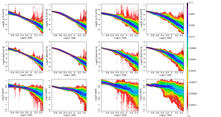
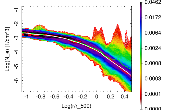
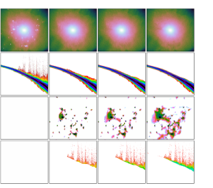
Using these data we generated Probability Density Function (PDF) of the ICM thermodynamic quantities in a set of radial shells for all clusters in the CSF and NR runs. The examples of the PDF for the relaxed cluster CL7 and unrelaxed cluster CL107 are shown in Fig. 1. The colour changing from red to dark-blue characterises the increasing volume-weighted probability of finding gas with a given density (or pressure/temperature) at a given radius. Overall radial trends of all thermodynamic properties are apparent from these plots. Moderate amplitude fluctuations of the ICM properties around these trends are visible as blue/green bands, which become broader with radius. Typically these bands account for $\sim$ 99 per cent of a shell volume. Below we refer to these bands as a volume-filling bulk component of the gas. Finally, high density inhomogeneities, occupying very small fraction of volume, are seen as red spikes. Another representation of both components is shown in the left panel in Fig. 2.

3 Characterizing the bulk component of the ICM

3.1 Median profiles

Figure 4: Width $W_{10}$ of the density (top panels) and pressure (bottom panels) distributions in a radial shell as a function of distance from the cluster center for CSF (left column) and NR (right column) simulations. The width is averaged over the sample of relaxed (black solid curves) and unrelaxed (red dashed curves) clusters. Thick solid and dashed curves correspond to the sample-averaged value and thin dotted curves show the scatter from cluster to cluster.

First, we would like to characterise overall radial profiles of the ICM thermodynamic properties, representing the bulk volume-filling component of the ICM. A primary application of these profiles is the cluster mass measurements via HSE equation.

Usually hot gas is characterized by the mean radial profiles of density and pressure obtained under the assumption of spherical symmetry. These profiles are used to determine the mass of the cluster using the HSE equation

$$\frac{1}{\rho}\frac{dP}{dr}=-\frac{GM}{r^{2}},$$ (1)

where $\rho$ and $P$ are radial profiles of gas density and pressure respectively and $M$ is the total gravitating mass of the cluster. If the pressure is due to the thermal gas pressure, then $P=nkT$ and $\rho=\mu m_{p}n$, where $\mu$ is the mean atomic weight of the gas particles, $m_{p}$ is the proton mass, $k$ is the Boltzmann constant and $n$ is the total particles density. Throughout the paper we use $\mu=0.588$. This procedure requires differentiation of the pressure over the radius. Thus the issue of a robust way of calculating radial pressure profiles is especially important. Various high density inhomogeneities affect the measurements of the mean radial profiles. Moreover, while the bulk of the gas may be close to the hydrostatic equilibrium in the cluster potential, the high density inhomogeneities are obviously far from equilibrium. Therefore in order to avoid spurious variations of the mean profiles due to high density inhomogeneities one has to excise them from the data. Often, when analyzing simulated data, the high density gas clumps are removed by introducing some threshold values in the density/temperature values and excising the regions where the ICM parameters violate these thresholds (e.g. Lau, Kravtsov, & Nagai, 2009; Vazza et al., 2011; Fabjan et al., 2011). The radial profiles are then calculated by averaging the density (or pressure/temperature), over the remaining volume. However, the resulting mean profiles are sensitive to the particular procedure of clump removal. High density inhomogeneities can significantly shift the mean density or temperature, causing distortions in the mean pressure. We instead are seeking a method which will be robust with respect to the presence of inhomogeneities and does not require fine tuning of the clump removal procedure.

We propose to use median radial profiles of density, temperature and pressure instead of their mean quantities as is most commonly done. Given N particles in a radial shell the calculation of the median is reduced to sorting particles in ascending/descending order and taking the value corresponding to a particle with index N/2. White curves in Figs. 1 and Fig. 3 show resulting median radial profiles. These median profiles can be favorably compared (Fig. 3) to the mean and mode profiles. The median profile is smooth and follows well the peak of the PDF even when contamination by high density gas inhomogeneities is very severe. Of course, this is true only as long as the fraction of volume occupied by the high density component is small. The mean density profile is reasonably smooth, but it is strongly affected by clumps, which drive it well above the PDF peak. The mode value by definition coincides with the peak of the PDF, but it is not smooth. Its fluctuations reflect (possibly small) variations of the PDF near the maximum.

Clearly the median value is an optimal choice if one thinks of using it for the hydrostatic equilibrium equation. It can be calculated straightforwardly from the PDFs in spherical shells without need to select or tune procedure of high density clumps removal. It characterizes directly the properties of the bulk component of the ICM and is not affected by the presence of high density inhomogeneities, as long as their volume fraction is small. The median pressure profile is a smooth function of radius, making it very suitable for the HSE equation.

3.2 Width of density and pressure distributions

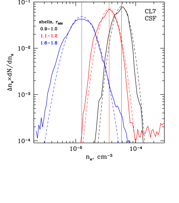
We now proceed with the evaluation of the width of the bulk component distribution. Fig. 2 (the right panel) shows the ICM density PDF in several radial shells. In some shells the density distributions are very asymmetric due to the presence of high density tails. However, if we exclude tails, the remaining distribution can be reasonably well described by a log-normal distribution around the median value

$$P(\ln x)d\ln x=\frac{1}{\sqrt{2\pi}\sigma}e^{\displaystyle-\frac{(\ln x-\ln x_{0})^{2}}{2\sigma^{2}}}d\ln x,$$ (2)

where $x_{0}$ is the median value, as illustrated in Fig. 2 (see also Kawahara et al., 2007). Even if we exclude high density tails, the distributions are quite broad, especially at large $r$. In Section 7 below we argue that the contribution of the overall ellipticity of the potential to the calculated width of the distribution does not exceed 20 per cent in relaxed clusters. We therefore refer to the broadening of the ICM density distribution in a radial shell around the medial values as “perturbations”.

Figure 5: Histogram of the width of the gas density distribution $W_{10}(n_{e})$ at $r_{500}$ for the CSF sample of relaxed clusters (cyan solid) and unrelaxed clusters (blue dashed). One can see two peaks in the distribution. The significance of the difference in width between two samples is $\sim 2.5\sigma$. The width $W_{10}\sim 0.3$ at $r_{500}$ divide clusters into relaxed/unrelaxed samples. This way of classification is independent of the projection effects.

Let us calculate the width of the density and pressure distributions - another important characteristic of the bulk component. We are seeking the procedure which is not very sensitive to the presence or absence of high density tail in the distribution. While the shape of the PDF of the bulk component is close to log-normal, small deviations are present. We therefore introduced an “effective full width half maximum”, $W_{10}$, as a proxy to the distribution width. The value of $W_{10}$ is calculated as follows. For each radial shell we find the value of density $n_{e,1}$ such that 12 per cent of points (volume) in this shell have the density smaller than $n_{e,1}$. Similarly we find $n_{e,2}$ such that 12 per cent of points (volume) have higher density than $n_{e,2}$. $W_{10}$ is then defined as:

$$W_{10}(n_{e})=\log_{10}\frac{n_{e,2}}{n_{e,1}}.$$ (3)

$W_{10}$ characterizes the logarithmic interval (10-based), which contain 76 per cent of points. Clearly, for a pure log-normal distribution $W_{10}$ is equal to FWHM ($\log_{10}$-based). This definition is also convenient, since numerically $\displaystyle W_{10}=\frac{2\sqrt{2\ln 2}}{\ln 10}\sigma\approx 1.02\sigma$, where $\sigma$ is the standard deviation (natural log based) of the log-normal distribution. With this definition of the width, the log-normal distribution, centered at the median value, provides reasonably good approximation of the bulk component PDF (see Fig. 2).

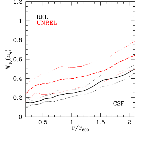
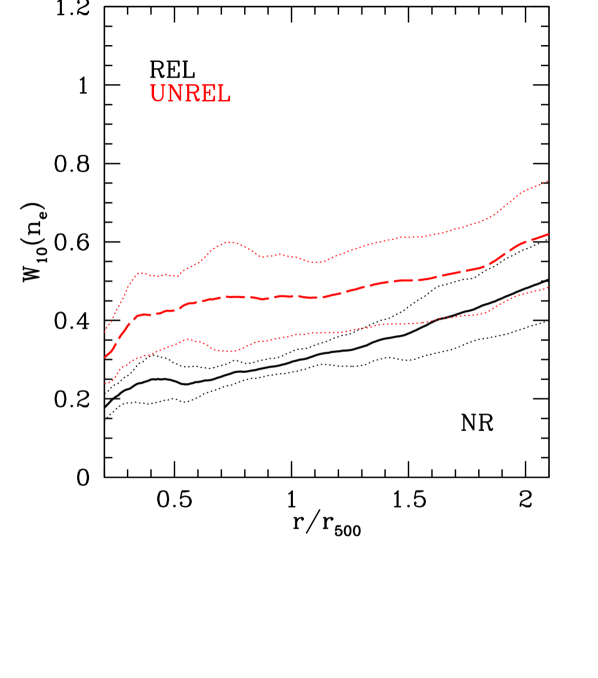
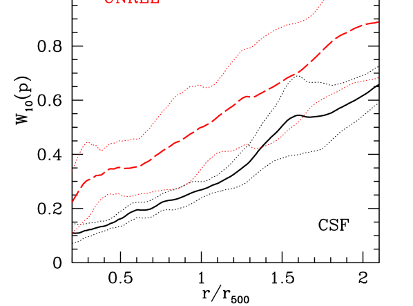
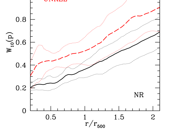
Fig. 4 shows the width of the distributions $W_{10}(n_{e})$ and $W_{10}(P)$ averaged over a sample of relaxed and unrelaxed galaxy clusters in CSF and NR runs. First we notice a strong increase of the width with radius $r$, which indicates that the gas is more inhomogeneous towards cluster outskirts. Scatter in the width from cluster to cluster is relatively small (especially for relaxed clusters). Pressure distributions are broader than density distributions at $r>r_{500}$, while at $r<r_{500}$ their widths are similar. Strong growth of the pressure width can be an indication of the gas deceleration at these radii. We refer readers to Section 7 for discussion on possible physical origin of the width of density and pressure distributions.

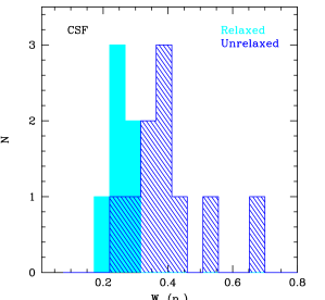
One can notice the tendency of unrelaxed clusters to have broader distribution of density and pressure than the relaxed clusters. This is not surprising, since any strong merger should perturb the density distribution. This tendency is even more clear if one looks at the histogram of $W_{10}(n_{e})$ at certain distance from the centre. Fig. 5 shows the corresponding histogram calculated at $r_{500}$ for relaxed and unrelaxed clusters in CSF run. Even though samples are small, the significance of the difference in width between two samples is $\sim 2.5\sigma$. It suggests a possibility of using the width $W_{10}$ at certain radius (e.g. $r_{500}$) as a criterion for an automatic division of clusters into broad relaxed/unrelaxed groups. Note that this way of classification is independent of the projection effects. Classification of all clusters into relaxed or unrelaxed objects in Nagai, Kravtsov, & Vikhlinin (2007) is based on the visual inspection of the mock X-ray images (see their Section 2). Further inspection of CL6 and CL9 clusters, identified as unrelaxed in Nagai, Kravtsov, & Vikhlinin (2007), but having relatively narrow density distribution ($W_{10}\leq 0.3$) shows that these objects can equally well be attributed to a class of relaxed objects within $r_{500}$.

4 Method to select high density inhomogeneities

Once we know the median density profile and the width of density distribution it is easy to separate the bulk component from the tails of the distribution. It additionally allows to study the properties of both components separately. We propose to use the following criterion of separation: particles with $\displaystyle\log_{10}n_{e}>\log_{10}\{n_{e}\}+f_{cut}\sigma_{10}$ are assigned to the high density tail, while all remaining particles belong to the bulk component. Here $\{n_{e}\}$ is the median value of the density and $\displaystyle\sigma_{10}=\frac{W_{10}}{2\sqrt{2\ln 2}}$ is the standard deviation ($\log_{10}$ based) of the density distribution. The choice of $f_{cut}$ is rather arbitrary. Experiments with simulated galaxy clusters in our sample show that $f_{cut}=3.5$ works well for both NR and CSF simulations. Clearly, by varying $f_{cut}$ one can select only the densest clump cores or the clumps together with the surrounding elevated density regions. These points are illustrated in Fig. 6, where we show density distributions and projected density maps obtained assuming different values of $f_{cut}=\infty$ (initial maps), $4.5,3.5$ and $2.5$. In the case of $f_{cut}=2.5$ we select not only “bona fide” high density tails, but also partially exclude particles, which belong to log-normal density distribution and characterize the bulk of the gas. In the case of $f_{cut}=4.5$ we separate only the top of densest clumps and attribute some of the substructure clearly related to clumps to the bulk gas.

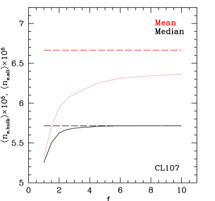
Here it is important to point out that the median profiles of the bulk component are essentially insensitive to the $f_{cut}$ value in comparison with the mean profiles. Fig. 7 illustrates this point for one cluster from the sample. We calculate median and mean radial profiles of the density in shells, removing different fractions of dense clumps (varying $f_{cut}$). Fig. 7 shows the mean and median values of the density of gas from simulations $n_{e,all}$ (both bulk gas and inhomogeneities) and the density of gas with excluded high density tail $n_{e,bulk}$ at $r_{500}$ as a function of cutoff $f_{cut}$. We see that once the $f_{cut}\geq 3$, the median is less sensitive to the presence of inhomogeneities and to various ways to exclude them than the mean.

Figure 6: Splitting of the ICM into high density inhomogeneities and bulk component of gas assuming different criteria of separation. Particles with $\displaystyle\log_{10}n_{e}>\log_{10}\{n_{e}\}+f_{cut}\sigma_{10}$, where $\sigma_{10}$ is the width of density distribution at each radial bin, are assigned to the high density component (Section 4). Remaining particles are assigned to the bulk component. Columns from the left to the right: $f_{cut}=\infty$(total gas) $,4.5,3.5,2.5$. Top row: projected density maps of the bulk component of gas, second row: PDF of the ICM density of the bulk component in radial shells as a function of distance from the cluster centre, third row: density maps of the high density inhomogeneities, bottom row: density distributions of the high density component in radial shells as a function of distance from the cluster centre. The figure suggests that $f_{cut}=3.5$ provides an optimum threshold for the division into bulk component and high density inhomogeneities – it removes only small fraction of particles and at the same time does not leave any obvious inhomogeneous features in the PDF.

5 Gas motions of the bulk component and the high density inhomogeneities

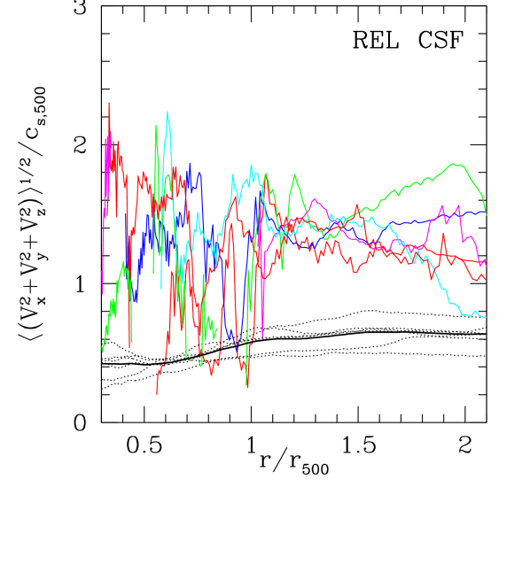
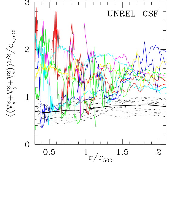
After splitting the ICM into two components it is easy to calculate characteristic velocities of the bulk component and of the high density inhomogeneities. As the reference velocity we use velocity averaged over the cluster core. Since in the present simulations the central $\sim$ 300 kpc region is strongly affected by the excessive gas cooling (e.g. Lau et al., 2012) that produces unphysical clumps moving with very high velocity, the average gas velocity within a wide radial shell at $400<r<500$ kpc was subtracted from the velocity field. Our experiments with different choices of region used to calculate the reference velocity have shown that final results are only weakly sensitive to this choice. The RMS velocity amplitude was calculated as $\sqrt{\langle V_{x}^{2}+V_{y}^{2}+V_{z}^{2}\rangle}$, where $\langle\rangle$ denotes averaging over the particles within a shell. Fig. 8 shows the ratio of the RMS velocity and the sound speed evaluated at $r_{500}$

$$c_{s,500}=\displaystyle\sqrt{\frac{\gamma kT_{500}}{\mu m_{p}}},$$ (4)

where $T_{500}$ is the gas temperature at $r_{500}$, $\gamma$ is the adiabatic index (for ideal monoatomic gas it is 5/3), $k$ is the Boltzmann constant, $\mu$ is the mean atomic weight and $m_{p}$ is the proton mass. One can notice that (i) RMS velocity of the bulk component has a very regular behaviour with distance from the cluster centre, while the velocities of the high density component vary strongly; (ii) the scatter of the velocities between individual clusters is small for the bulk component and is on the contrary very large for the dense inhomogeneities; (iii) on average dense clumps move faster than the bulk component. Such behaviour of the RMS velocity in both components is not surprising. The bulk component is close to the HSE, while high density inhomogeneities are far from equilibrium. Note that for high density inhomogeneities $\displaystyle\frac{V_{rms}}{c_{s,500}}\approx 1$ at $r_{500}$. This means that the clumps’ kinetic energy is about the same as the thermal energy per unit mass in the bulk component. This is expected for the gas that has been heated by the thermalization of the bulk gas motions with velocities comparable to the observed velocities of the strongly overdense clumps (Felten et al., 1966).

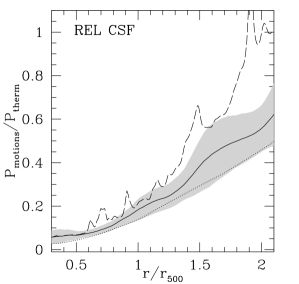
We also gauge how strongly high density inhomogeneities affect the ratio of thermal pressure and the “pressure” due to stochastic gas motions. The ratio of pressures is given by

$$\frac{P_{motions}}{P_{thermal}}=\displaystyle\frac{\langle\displaystyle\frac{1}{3}\rho V_{amp}^{2}\rangle}{\{nkT\}},$$ (5)

where $V_{amp}$ is the RMS velocity amplitude (see Fig. 8), $\langle\rangle$ and $\{\}$ denote mean and median values of pressure respectively. As an example, we show this ratio as a function of $r$ for relaxed CSF clusters in Fig. 9. Contribution of the pressure due to gas motions to the thermal pressure is $\sim$ 5 per cent in the cluster centre and increases with radius. Exclusion of high density inhomogeneities leads to a significantly smaller ratio at $r>r_{500}$. Once again this demonstrates that the bulk component is much closer to the HSE, than the ICM inhomogeneities. Comparison with previous results from Lau, Kravtsov, & Nagai (2009) shows a broad agreement (dotted and dashed curves in Fig. 9). Small discrepancies in radial profiles are mostly due to different ways to subtract the mean velocity from the total velocity field. We subtract the mean velocity in radial shell $400<r<500$ kpc as described above, while Lau, Kravtsov, & Nagai (2009) subtract mean velocity in each radial shell. Also discrepancies in pressure ratio are due to different procedures of clump exclusion and slight distinction between median and mean thermal pressures.

Figure 7: Sensitivity of the median (black) and mean (red) values of the density to the cutoff value, used to separate the bulk and high density components. Dashed curves show the mean and median values of the total density from simulations $\langle n_{e,all}\rangle$ at $r_{500}$. Dotted and solid curves show density of the bulk gas at $r_{500}$ as a function of $f_{cut}$. Large $f_{cut}$ excludes only the densest inhomogeneities, while very small $f_{cut}$ can exclude in addition slightly overdense gas, belonging to the bulk component (see Fig. 6). Closeness of the black curves over a broad range of $f_{cut}$ implies that the median is not sensitive to the particular value of the cutoff, unless it is very low. In contrast, the value of the mean density is much more strongly affected by the presence of rare high density inhomogeneities and by the choice of the threshold $f_{cut}$ used to excise the inhomogeneities.

6 Clumping factor with and without dense inhomogeneities

We calculated the clumping factor, which characterizes distortions in the X-ray flux from a given shell, relative to the flux calculated using the median temperature and density values in the same shell. This factor is:

$$C_{X}=\displaystyle\frac{\displaystyle\langle\Lambda(T)n_{e}^{2}\rangle}{\displaystyle\{\sqrt{\Lambda(T)}n_{e}\}^{2}},$$ (6)

where $\Lambda(T)$ is emissivity in a given energy band as a function of temperature, $\langle\rangle$ and $\{\}$ denote mean and median values respectively. The emissivity as a function of temperature was calculated for the 0.5-2 keV energy band - where the sensitivity of current X-ray observatories is close to maximal for a typical cluster spectrum.

The choice of the emissivity-weighted clumping factor $C_{X}$ instead of the “classical” clumping $\langle n_{e}^{2}\rangle/\langle n_{e}\rangle^{2}$ is motivated mainly by the two reasons. First, emissivity factor automatically takes care of the exclusion of the densest and coldest gas clumps present in simulations. Thus we do not need to introduce a cut over the temperature to calculate clumping for X-ray emitting gas (e.g. Nagai & Lau, 2011). Secondly, median value in denominator in eq. (6) is characteristics of the hydrostatic component in the ICM. Therefore, clumping factor $C_{X}$ reflects the increase of the surface brightness due to inhomogeneities in the ICM relative to the surface brightness in an ideal hydrostatic situation. We conclude that calculation of the clumping factor using eq. 6 has good physical motivation.

Fig. 10 shows clumping factor calculated for the total gas in simulations and for the bulk nearly hydrostatic component. As expected, the exclusion of high density inhomogeneities significantly modifies the clumping factor: clumping factor becomes smaller, especially at $r>r_{500}$ and smoother with radius. Both curves determine the upper and lower limits on the boost of X-ray flux over the flux in the bulk gas we expect to find in X-ray observations. Nagai & Lau (2011) calculated the clumping factor for gas with $T>10^{6}$ K. Such a temperature cut partially excludes high density inhomogeneities in the ICM. Comparison shows that the clumping factor from Nagai & Lau (2011) is in between dashed and solid curves. As an example, we show their measurements for relaxed clusters in CSF simulations with dotted curve in Fig. 10.

The clumping factor, calculated using eq. 6, directly characterizes the increase of the surface brightness in the 0.5-2 keV band due to overall ellipticity and inhomogeneities in the ICM. Inspection of the mock images suggests that very bright and localized regions are responsible for high values of $C_{X}$ when the bulk and high density components are considered together (dashed line in Fig. 10). This means that simple cleaning of X-ray images from the most obvious bright spots should bring the clumpiness factor down to the values characteristic for the bulk component (solid line in Fig. 10).

Table 2: Clumping factor calculated using eq. (6) for total gas from simulations and bulk gas only at $r_{500}$ and $1.5~{}r_{500}$. See also Fig. 10. For comparison, we show clumping factors in PKS 0745-191 (Walker et al., 2012) and Perseus (Simionescu et al., 2011) clusters calculated from the observed overestimation factor of the gas density.

gas component	$C_{X}$	$C_{X}$
	at $r_{500}$	at $1.5~{}r_{500}$
CSF REL
Total	1.2	1.6
Bulk	1.1	1.3
NR REL
Total	1.6	3.1
Bulk	1.2	1.4
CSF UNREL
Total	1.6	1.9
Bulk	1.4	1.6
NR UNREL
Total	2.2	2.7
Bulk	1.7	1.8
PKS 0745-191	$\sim$ 1-3	$\sim$ 2-9
Perseus	$\sim$ 1-3	$\sim$ 9-12

Figure 8: Ratio of the RMS velocity amplitude (averaged in shells) and the sound speed at $r_{500}$ as a function of distance from the cluster centre. The sound speed at $r_{500}$ is calculated as $\displaystyle c_{s,500}=\displaystyle\sqrt{\gamma kT_{500}/\mu m_{p}}$ (see Section 5 for details). Solid coloured curves: ratio for the dense inhomogeneities only, different colours correspond to different clusters. Dotted black curves: ratio for the bulk gas component. Thick solid black curves: ratio for bulk component of gas, averaged over the sample of relaxed (left panel) or unrelaxed (right panel) clusters. Note that on average clumps are moving with larger velocity than the gas in the bulk component.

For hot clusters the temperature dependence of the emissivity is usually neglected and the increase of the surface brightness directly translates into the overestimation of the density by a factor $\displaystyle\sqrt{C_{X}}$. This quantity is especially important when the resulting density profile is used to infer the gas mass or the ratio of the gas mass to the total mass, i.e. $f_{gas}$. From this point of view it is interesting to compare the results of the simulations with the suggested overestimation factor of the gas density from the X-ray observations. For the Perseus cluster this factor is $\sim$ 1-1.6 at $r_{500}$ and increases to $\sim$ 3-3.4 by $1.5~{}r_{500}$ (Simionescu et al., 2011). Corresponding value in terms of $C_{X}$ is the square of this factor, i.e. $C_{X}\approx 1-2$ and $\approx 9-12$ at these two radii respectively. For the PKS 0745-191 cluster clumping factor $C_{X}\approx 1-3$ and 2-9 at $r_{500}$ and $1.5~{}r_{500}$ respectively (Walker et al., 2012). Since the most prominent high density peaks were excluded from the X-ray images of both clusters, these values of the clumping factor should be close to the values for the bulk gas in simulations. Table LABEL:tab:clumping shows values of the clumping factor from the simulated clusters in our sample at $r_{500}$ and $1.5~{}r_{500}$. One can notice that there is an agreement between simulations and observations at $r_{500}$. At $1.5~{}r_{500}$ simulations are marginally consistent with clumping factor in the PKS 0745-191 cluster. However, values for the Perseus cluster are larger at $1.5~{}r_{500}$ than found in simulations especially if relaxed sample is considered.

The difference between observations and simulations can be due to several reasons. The high clumping factor in the Perseus cluster was inferred from a narrow stripe along the NW arm of the cluster. Hydrodynamical simulations indicate that the distribution of gas clumps is highly anisotropic, azimuthal scatter of the clumping factor is large (Eckert et al., 2012). It is therefore possible that the clumping factor along the given direction is larger than the azimuthally averaged value. We note that clumping factor for the PKS 0745-191 is averaged over five directions and is in a better agreement with simulations. Another possible reason of the higher clumping factor in the X-ray data is the contamination by unresolved sources in low surface brightness regions. The spatial resolution of Suzaku is limited and it is difficult to properly model the contribution of background (AGNs) which could lead to contamination and hence the over-estimate of the gas density in low surface brightness regions in cluster outskirts. Indeed, it was shown recently that the clumping factor measured in simulations is sufficient for describing the excess of the gas density measured with ROSAT observatory in cluster outskirts (Eckert et al., 2012). Clearly, more work from both simulations and observations is needed to resolve the issues discussed above.

Figure 9: Ratio of the pressure due to gas motions and the gas thermal pressure as a function of distance from the cluster centre, averaged over a sample of relaxed clusters in the CSF run. Dashed curve: pressure ratio for total gas distribution (bulk plus high density inhomogeneities) from simulations. Solid curve: the ratio for the bulk component. Gray shadow: scatter of the ratio for the bulk component. Dotted curve: pressure ratio from Lau, Kravtsov, & Nagai (2009). See Section 5 for details.

7 Origin of the density fluctuations in the bulk component

Gas density inhomogeneities should cause observable fluctuations of the surface brightness in the X-ray images of galaxy clusters. For hot $T>3~{}{\rm keV}$ gas the X-ray emissivity weakly depends on temperature or metal abundance. Therefore X-ray surface brightness fluctuations are a direct proxy for the density inhomogeneities. Recent analysis of the surface brightness fluctuations in the Coma cluster shows that the typical amplitude of density perturbations (RMS) on scales from 30-500 kpc ranges from 5 per cent to 10 per cent (Churazov et al., 2012). This is in a reasonably good agreement with the amplitude of density fluctuations we see in simulations (Fig. 4) in relaxed clusters. While Coma is not very relaxed cluster, the central part studied with Chandra and XMM-Newton is reasonably relaxed. Broad agreement between simulations and observations is encouraging and suggests that the simulations might correctly capturing the physics responsible for the density fluctuations. We now proceed with the discussion of the key properties of the density inhomogeneities in the simulations.

In the majority of radial shells the density distribution has two distinct components: (i) log-normal distribution with a substantial width, and (ii) a high density tail. The latter component is often associated with the cold and dense gas in subhalos. This component is more prominent in the CSF simulations. This is not surprising given that the radiative cooling time of the dense gas can be short.

The width of the log-normal “bulk” component is substantial (see Fig. 2 and 4) – the mean value of $W_{10}$ at $r_{500}$ varies between 0.15 and 0.5 in most of the relaxed cluster. Clearly, the width is expected to be zero if the potential is spherical and static, the gas is in equilibrium and radial shells are infinitely narrow. An interesting question is to understand the properties of the density fluctuations in the bulk component that cause broadening of the density distributions. Below we analyze the properties of these fluctuations.

7.1 Finite thickness of radial shells

We first address the question if the observed spread of densities in a shell is a spurious effect of the shell finite thickness. Assuming that locally the number density is a power law function of radius $n_{e}(r)\propto r^{-\alpha}$, the upper limit on the total width (from the minimal to the maximal value) is

$$W_{tot}=\displaystyle log_{10}\left(\frac{n(r)}{n(r+\displaystyle\Delta r)}\right)\approx\displaystyle\frac{\alpha\frac{\Delta r}{r}}{\ln 10}.$$ (7)

In our calculations $\displaystyle\frac{\Delta r}{r}\approx 0.01$ and the slope $\alpha$ of the gas density varies from $\approx 1$ in the centre to $\approx 3$ at $2~{}r_{500}$. Therefore, in this case an upper limit on $W_{10}<W_{tot}$ due to the finite thickness of shells is $\sim 1$ per cent. We conclude that no significant contribution to the width of the density distribution is caused by the shell finite thickness.

7.2 Ellipticity and perturbations of the potential

Another plausible reason for the observed variations of the gas density in a spherical shell is the overall ellipticity/asphericity of the cluster. One can use the known gravitational potential of the cluster, created by dark matter and baryons, as a proxy to the underlying ellipticity. For instance, one can imagine a situation when essentially hydrostatic gas is sitting in an elliptical potential well.

For the isothermal gas in hydrostatic equilibrium the number density $n_{e}$ is related to the static potential $\phi$ through the Boltzmann distribution $n_{e}\propto e^{-\frac{\phi\mu m_{p}}{kT}}$. Let us calculate a correlation coefficient $C$ between density $\displaystyle\delta\ln n_{e}$ and potential $\displaystyle\delta\phi$ variations in a shell. We define the correlation coefficient $C(x,y)$ between two variables $x$ and $y$ in a usual way:

$$C(x,y)=C(y,x)=\frac{\langle xy\rangle}{\sigma_{x}\sigma_{y}}=\frac{\sum\limits_{i}x_{i}y_{i}}{\sqrt{\sum\limits_{i}x_{i}x_{i}}\sqrt{\sum\limits_{i}y_{i}y_{i}}},$$ (8)

where $\sigma_{x}$ and $\sigma_{y}$ are the dispersions of $x$ and $y$ respectively; both variables are assumed to have zero mean; $\langle\rangle$ denotes averaging over all particles in the shell.

Figure 10: Clumping factor (eq. 6) as a function of radius, averaged over our samples of relaxed/unrelaxed clusters. Dashed: full gas distribution (bulk plus inhomogeneities), solid: bulk component. Dotted: clumping factor from Nagai & Lau (2011). See Section 6 for details.

Fig. 11 shows the correlation coefficient $\displaystyle C(\ln n_{e},\phi_{c})$ (hereafter $\phi_{c}=\phi\displaystyle\frac{\mu m_{p}}{kT_{med}}$) between density and potential fluctuations for the CF and NR runs averaged over samples of relaxed and unrelaxed clusters. Clearly, if the isothermal gas is in equilibrium in a static gravitational potential, then $\displaystyle\delta\ln n_{e}=-\phi\frac{\mu m_{p}}{kT_{med}}$ and the correlation coefficient is $-1$. In the opposite case $C=1$. However, we see that in simulations the correlation coefficient in most cases is between $\approx-0.6$ and $\approx-0.4$, except for relaxed clusters in the NR simulations, where the correlation coefficient reaches $\approx-0.86$ in the central $r\leq 0.5r_{500}$. This means that the asphericity of the potential can not alone at a given moment of time explain all observed density variations. For instance, non-isothermality of the gas in shells could contribute to the density variations.

Knowing the correlation coefficient between the density and potential one can calculate the width of the density distribution $W_{10,\phi}$ corrected for the potential variations in the shell. Indeed, let us assume that we want to account for correlation between variables $x$ and $y$ and construct new variable $y^{\prime}=y-R(x,y)\times x$ with minimal dispersion. We seek the regression coefficient $R(x,y)$ which minimizes $\langle y^{\prime 2}\rangle$. This regression coefficient is (assuming again that both variables have zero mean)

$$R(x,y)=\frac{\sum x_{i}y_{i}}{\sum x_{i}x_{i}}.$$ (9)

The dispersion of $y^{\prime}$ is then $\sigma^{2}_{y^{\prime}}=\sigma^{2}_{y}-C(x,y)^{2}\sigma^{2}_{y}$. Thus, one can calculate the width of the density distribution $W_{10,\phi}$ through the correlation coefficient between the density and potential as

$$W_{10,\phi}=W_{10}\sqrt{1-C(\ln n_{e},\phi_{c})^{2}}.$$ (10)

Therefore, from the value of the correlation function $|C(\ln n_{e},\phi_{c})|=0.4-0.6$ it follows that accounting for the potential variations in a shell reduces the width of the log-normal density distribution by a factor $\displaystyle\frac{W_{10}-W_{10,\phi}}{W_{10}}=1-\sqrt{1-C^{2}}\approx 8-20\%$.

Overall ellipticity of the mass distribution is not the only reason for potential variations in a spherical shell. The variations can also be caused by the presence of subhalos. However the cores of the most prominent and gas rich subhalos have been excluded as high density inhomogeneities, leaving only outer regions of the subhalos as a possible contributor to the bulk component density variations. The above estimate includes both types of variations and can be used as an upper limit on the variations induced by the ellipticity.

The bottom line of this exercise is that in the simulations only a small part of the density variations in spherical shells can be attributed to the ellipticity/asphericity of the underlying potential, under the assumption that it is static.

7.3 Adiabatic and isobaric fluctuations

We now address the question if the observed density variations in the bulk gas component are predominantly adiabatic or isobaric. Adiabatic fluctuations arise from sound waves or weak shocks (and can be associated with the variations of the potential with a shell), while isobaric fluctuations naturally appear when gases with different entropies are brought to contact e.g. by ram pressure stripping or turbulent gas motions.

To answer this question we calculate the regression coefficient $R$ defined by eq. 9 between density variations and temperature or pressure variations (Fig. 12). If density fluctuations are purely adiabatic, then the regression coefficient $R(\ln n_{e},\ln T)=1/(\gamma-1)=1.5$ and $R(\ln n_{e},\ln P)=1/\gamma=0.6$. In the case of pure isobaric density fluctuations, $R(\ln n_{e},\ln T)=-1$ and, obviously, $R(\ln n_{e},\ln P)=0$. One can see in Fig. 12 that the sample-averaged (over sample of relaxed CSF clusters) regression coefficient does not correspond to the value characteristic for pure adiabatic or isobaric density fluctuations. This conclusion remains valid for unrelaxed clusters and for NR runs as well. In individual clusters the scatter in the regression (and correlation) coefficients is large. The value of $R(\ln n_{e},\ln T)$ varies from -0.8 up to 0.5, i.e. in some cases $R$ approaches values characteristic for pure isobaric fluctuations. Inspection of individual clusters shows that these low/high values of $\displaystyle C(\ln n_{e},\ln T)$ at some radii are often driven by some distinct feature, like an outskirt of a subhalo or a moderately strong shock.

Figure 11: Radial profiles of the correlation coefficient (eq. 8) between the density fluctuations $ln(n_{e})$ and fluctuations of potential $\phi_{c}=\phi\displaystyle\frac{\mu m_{p}}{kT_{med}}$ (solid curves) or temperature $ln(T)$ (dashed curves). The data are averaged over subsamples of NR/CSF and relaxed/unrelaxed clusters. See Sections 7.2 and 7.3 for details.

Figure 12: Radial profiles of the regression coefficient (eq. 9) between the density fluctuations and temperature or pressure fluctuations. The profiles are averaged over a sample of relaxed CSF clusters. Dotted lines show the regression coefficient in cases of pure adiabatic and pure isobaric fluctuation. The sample-averaged regression coefficients do not show the values characteristic for pure adiabatic or pure isobaric fluctuations of density. See Section 7.3 for details.

7.4 General comments on the density variations

As we discussed above the asphericity of the gravitational potential at a given moment can account up to 20 per cent of the bulk component density variations in narrow radial shells.

Another likely reason for the density variations is directly related to gas motions. From Fig. 8 it is clear that the gas motions in the bulk component are predominantly subsonic. We are therefore dealing with a weakly compressible case. Any given velocity field can be decomposed into solenoidal and compressible parts, both of which can contribute to the observed variations of density and pressure. A crude estimate of the density variations caused by variations of the square of the gas velocity is possible using Bernoulli’s equation: $\displaystyle\frac{\delta P}{P}\propto M^{2}$, where $M$ is a characteristic Mach number of isotropic turbulent gas motions $\displaystyle M^{2}=\frac{\langle v_{x}^{2}+v_{y}^{2}+v_{z}^{2}\rangle}{c_{s}^{2}}$ (Landau & Lifshitz, 1959). Assuming that the density fluctuations are adiabatic, i.e. $\displaystyle\frac{\delta n}{n}\propto\frac{1}{\gamma}\frac{\delta P}{P}$ one can expect $\displaystyle\frac{\delta n}{n}\approx\frac{\alpha}{3}M^{2}$, where $\alpha$ is of order unity. For an order of magnitude estimate one can adopt the value of $\alpha\approx 0.7$, calculated for incompressible gas (e.g. Hinze, 1975). The Mach number evaluated for the bulk flow is $\sim 0.55$ at $r_{500}$ for relaxed clusters in both CSF and NR simulations (see Fig. 8). Therefore, $\displaystyle W_{10}\approx\frac{\delta n}{n}\approx 0.07$ at $r_{500}$. This means that variations of the square of the gas velocity can explain $\sim 30$ per cent of the width of density distribution found in simulations.

The contribution of pure compressible motions to the density variations scales linearly with the Mach number $M$. To evaluate it properly one has to make Helmholtz decomposition of the velocity field. This is beyond the scope of this paper. We instead note that both solenoidal and compressible modes in the subsonic case should lead to adiabatic relation between density and pressure (or temperature) fluctuations. As we saw above (§7.3) the mean density/temperature regression coefficient (see Fig.11) is not close to 1.5. We further estimated the mean correlation coefficient $\displaystyle C(\ln n_{e},\ln P)\sim 0.7$ between the density and pressure fluctuations at $r_{500}$ for a sample of relaxed clusters. This corresponds to $\sim$ 30 per cent of the observed density variations, placing constraints on both solenoidal and compressible modes together. Therefore pure adiabatic fluctuations alone are not able to explain the density variations found in simulations and substantial contribution should be associated with the entropy variations.

Indeed, time variations of the potential and gas motions can also be responsible for inhomogeneity of the gas in radial shells, when the gas with an entropy different from the mean/median gas entropy at a given radius is advected to this radius. One can identify two flavors of this process. First, the motion of a subhalo can be responsible for the transportation of the gas. This process is also accompanied by a ram pressure stripping and partial mixing of the gas with the ICM. Second, the gas motions themselves can displace lumps of gas with different entropies from their “equilibrium” radius. The morphology of a moderately overdense gas component, corresponding to 2-3 $\sigma$ deviations from the median value (see §4) traces the distribution of subhalos, suggesting the first mechanism as a primary contributor. At smaller density contrasts $\leq 1~{}\sigma$ it is difficult to draw firm conclusion. Most likely both mechanisms play a role in producing nonuniform density in radial shells. Inspection of Fig. 11 suggests that at least in the central region $r<r_{500}$ apparent anti-correlation of the density and temperature variations is driven by these mechanisms.

8 Sensitivity of results to physics included in simulations

Our analysis was applied to simulated galaxy clusters with different physics included. We expect the real characteristics of the ICM gas to be somewhere in between CSF and NR cases. It is therefore interesting to examine which quantities, studied here, changes strongly between CSF and NR runs.

In general, gas cooling in CFS runs should lead to a more dense and prominent core at the cluster centre. The off-centre clumps are also expected to be denser and more compact. These effects reveal themselves as a “forest” of high density peaks in the density distribution in the CFS runs (see Fig. 1). The impact of the cooling on the bulk component is much more subtle, as summarized below for a subsample of relaxed clusters:

• The difference between the mean width of density and pressure distributions in the CSF and NR runs is minor. At $r_{500}$ the mean width of density distributions in relaxed clusters is $\sim$ 16 per cent larger in NR runs than in the CSF ones. The difference in the width could be due to the difference in ellipticity of the gas distribution (see Lau et al., 2011, 2012). Indeed, after correction for the contribution of the ellipticity, using the approach, outlined in §7.2, the difference in the width of the distributions in the NR and CSF runs near $r_{500}$ reduces down to $\sim$4 per cent.

• The RMS velocities in the bulk component or the ratio $\displaystyle\frac{P_{motions}}{P_{thermal}}$ are very similar in both runs.

• The clumping factor (see eq. 6), calculated for the bulk component at $r_{500}$ is $\sim 23$ per cent and $\sim 8$ per cent higher in the NR runs for unrelaxed and relaxed clusters respectively. The clumping factor, calculated for total density distribution including the high density tail is also larger for NR run. In this case the difference can be up to 40 per cent. The clumping factor is sensitive to cluster classification on relaxed and unrelaxed systems and has a very large scatter from cluster to cluster. Even after averaging over the sample, one object can dominate the mean.

This difference between CSF and NR can be understood in terms of a simple notion: in CSF runs the gas with high or intermediate densities has a short cooling time. This gas cools down below X-ray temperatures resulting in a stronger separation of hot and low density gas and much colder clumps. While in the NR runs the gas at intermediate densities/temperatures has much longer life time.

9 Summary

In this study we propose a novel description of the ICM in simulated galaxy clusters that allows us to better understand the properties of the bulk of the hot gas in clusters and various inhomogeneities. Our analysis is applied to 16 simulated galaxy clusters with different baryonic physics. The main results and conclusions can be summarized as follows.

1. We suggest a simple, quick and robust method to divide the ICM in simulations into a nearly hydrostatic bulk component and non-hydrostatic high density inhomogeneities. This allows us to study separately the properties of both components. In X-ray observations similar division between these two components is usually based on the analysis of X-ray images from which bright localized spots are excluded. The selection of the bulk component implemented in the present study corresponds to the idealized case, when statistical quality of the data allows one to make careful cleaning of the image from all distinct features. The analysis of two components together corresponds to another limit when no bright spots are excluded from observed images.

2. The characteristic amplitude of stochastic gas velocities in the bulk component is increasing with radius and has a very regular behavior. RMS velocity averaged over a sample of relaxed (unrelaxed) clusters varies from $\sim 0.4~{}c_{s,500}(\sim 0.7~{}c_{s,500})$ at $0.3~{}r_{500}$ to $\sim 0.6~{}c_{s,500}(\sim 0.8~{}c_{s,500})$ at $2~{}r_{500}$. This is in a broad agreement with previous measurements (e.g. Lau, Kravtsov, & Nagai, 2009). Velocities of motions in the high density component, in contrast, are higher, change irregularly with radius and exhibit large scatter from one cluster to another. Note that the values of velocities in the bulk gas component are consistent with current velocity estimates from X-ray observations (e.g. Werner et al., 2009; Sanders, Fabian, & Smith, 2011; de Plaa et al., 2012). The forthcoming Astro-H mission (launch date 2014) will provide more robust constraints on the gas velocities since it has high energy resolution $\sim 5$ eV. E.g. in Zhuravleva et al. (2012) we show that in the Perseus-like clusters gas motions with $V_{gas}\gtrsim 0.3c_{s}$ cause line broadening of $\sim$ 7 eV, while the thermal broadening does not exceed 3 eV. Therefore, gas motions should be readily detectable.

A closely related quantity is the ratio of pressure due to gas motions and thermal pressure, which is $\sim 0.2$ at $r_{500}$ for relaxed clusters. This result holds for bulk component alone and for the bulk plus high density components together. At larger radii the ratio $\displaystyle\frac{P_{motions}}{P_{thermal}}$ in the bulk component is increasing gradually to 50-60 per cent at $2~{}r_{500}$ for relaxed clusters (and even more for the bulk plus high density components together).

3. The clumping factor boosts the X-ray emissivity for the bulk component in relaxed clusters by less than $\sim$15-25 per cent within $r_{500}$. This factor increases to 30-40 per cent at $2~{}r_{500}$. For the bulk plus high density components together the clumping factor is much larger and is very irregular.

4. We introduce two characteristics of the bulk component: median radial profiles of density/temperature/pressure - characteristic of the overall radial properties and width $W_{10}$ of the density and pressure distributions - characteristic of gas fluctuations around the median value.

In contrast to the mean, mode or range profiles, the median profiles are very robust even if the ICM is strongly contaminated by high density inhomogeneities. Therefore, in order to calculate radial profiles of gas characteristics, we do not need to exclude clumps from the ICM first. This would significantly simplify analysis of big samples of simulated clusters.

The density distribution of the bulk gas in each radial shell can be well described by log-normal distribution. We propose to use the width of density distributions as another robust characteristic of the bulk gas. The width is an increasing function of distance from the cluster centre with a relatively small scatter from cluster to cluster, especially for relaxed clusters. The typical width of the density distribution at $r_{500}$ in our CSF sample is $W_{10}\sim 0.25$ dex with the scatter $\pm 0.037$ for relaxed clusters, while for unrelaxed clusters the typical width is $\sim 0.43$ dex with slightly larger scatter $\pm 0.14$. This suggests that the width can be used as an additional criterion to classify clusters in large simulations into relaxed and unrelaxed clusters.

5. We investigated the properties of the density inhomogeneities in the simulated sample. The ellipticity of the underlying mass distribution can explain $8-20$ per cent of the observed density variations of the bulk component in individual clusters at $r_{500}$. Another $\sim 30$ per cent of the density distribution width $W_{10}$ at $r_{500}$ can be attributed to the adiabatic pressure/density variations in the turbulent ICM. The remaining part of the observed density variations in the bulk component is associated with the variations of gas entropy at a given distance from the cluster centre. These entropy variations are likely caused by advection of the gas by moving subhalos, including the ram-pressure stripped gas, and by gas advection by stochastic gas motions.

6. Compared to observations, the width of the gas density distribution in the inner parts of relaxed clusters $W_{10}\sim 0.1-0.2$ dex (FWHM), broadly agrees with the typical amplitude of density perturbations of 5 per cent to 10 per cent (RMS) in the Coma cluster core (Churazov et al., 2012). In the cool-core AWM4 cluster, which is probably more relaxed than Coma, Sanders & Fabian (2012) found 4 per cent density variations. Further analysis of a sample of cluster is needed to conclude if additional processes like thermal conduction or mixing are required to reduce the ICM inhomogeneity in simulations. The clumping factor $C_{X}\sim 1.1-2.2$ at $r_{500}$ found in the simulations is in agreement with the value 1-3 suggested by the observations. However, at cluster outskirts ($1.5~{}r_{500}$) clumping from the simulations broadly agrees with observations of PKS0745-191 cluster (Walker et al., 2012) but is $\sim 3$ times smaller than the clumping factor in the Perseus cluster(Simionescu et al., 2011).

While this paper was in review, we noticed another paper by Battaglia et al. (2012), where the measurement biases of $f_{gas}$ were analyzed using another sample of simulated clusters. In their paper Battaglia et al. (2012) used $T>10^{6}$K cut in the calculation of the clumping factor to mimic the X-ray observations (cf. eq. 6) and provide the value of $f_{gas}$ within given radius. Crude estimates show that the behavior of the clumping factor is qualitatively similar to our results for the case when high density inhomogeneities are not excluded (dashed line in Fig.10).

7. The analysis described in the paper has important implications for the measurements of the total mass of clusters. Separation of the high density tail from the bulk component of the ICM, allows one to plug into HSE equation quantities that are not contaminated by various gas inhomogeneities. This provides a lower limit on the mass bias one can obtain from the standard analysis of X-ray observations, once all substructures are carefully removed from the data. This issue will be addressed in our future work. Also, a combination of the median density and temperature radial profiles along with the width of their distributions provides a convenient way to calculate other possible biases in the observables, such as the bias in the X-ray emissivity or X-ray temperature and pressure measured through the SZ effect (see Khedekar et al., 2012).

10 Acknowledgements

IZ, EC, AK, DN and EL thank KITP for hospitality during the workshop “Galaxy Clusters: the Crossroads of Astrophysics and Cosmology”(2011). The work was supported in part by the Division of Physical Sciences of the RAS (the program “Active processes in galactic and extragalactic objects”, OFN-17). AK was supported in part by NSF grants AST-0807444, NASA grant NAG5-13274, and by the Kavli Institute for Cosmological Physics at the University of Chicago through the NSF grant PHY-0551142 and PHY-1125897 and an endowment from the Kavli Foundation. EL was supported in part by NASA Chandra Theory grant GO213004B. DN acknowledges support from NSF grant AST-1009811, NASA ATP grant NNX11AE07G, NASA Chandra Theory grant GO213004B, Research Corporation, and Yale University. This work was supported in part by the facilities and staff of the Yale University Faculty of Arts and Sciences High Performance Computing Center. The cosmological simulations used in this study were performed on the IBM RS/6000 SP4 system (copper) at the National Center for Supercomputing Applications (NCSA).

References

- Allen et al. (2004) Allen S. W., Schmidt R. W., Ebeling H., Fabian A. C., van Speybroeck L., 2004, MNRAS, 353, 457
- Battaglia et al. (2012) Battaglia N., Bond J. R., Pfrommer C., Sievers J. L., 2012, arXiv:1209.4082
- Churazov et al. (2012) Churazov E., et al., 2012, MNRAS, 421, 1123
- de Plaa et al. (2012) de Plaa J., Zhuravleva I., Werner N., Kaastra J. S., Churazov E., Smith R. K., Raassen A. J. J., Grange Y. G., 2012, A&A, 539, A34
- Eckert et al. (2012) Eckert D., et al., 2012, A&A, 541, A57
- Fabjan et al. (2011) Fabjan D., Borgani S., Rasia E., Bonafede A., Dolag K., Murante G., Tornatore L., 2011, MNRAS, 416, 801
- Felten et al. (1966) Felten J. E., Gould R. J., Stein W. A., Woolf N. J., 1966, ApJ, 146, 955
- Haiman, Mohr, & Holder (2001) Haiman Z., Mohr J. J., Holder G. P., 2001, ApJ, 553, 545
- Hinze (1975) Hinze, J. O., 1975, Turbulence, Mc-Graw-Hill Inc., chapter 3
- Kawahara et al. (2007) Kawahara H., Suto Y., Kitayama T., Sasaki S., Shimizu M., Rasia E., Dolag K., 2007, ApJ, 659, 257
- Khedekar et al. (2012) Khedekar S. et al., 2012, MNRAS, in prep.
- Kravtsov, Klypin, & Hoffman (2002) Kravtsov A. V., Klypin A., Hoffman Y., 2002, ApJ, 571, 563
- Kravtsov, Klypin, & Khokhlov (1997) Kravtsov A. V., Klypin A. A., Khokhlov A. M., 1997, ApJS, 111, 73
- Kravtsov, Vikhlinin, & Nagai (2006) Kravtsov A. V., Vikhlinin A., Nagai D., 2006, ApJ, 650, 128
- Mathiesen, Evrard, & Mohr (1999) Mathiesen B., Evrard A. E., Mohr J. J., 1999, ApJ, 520, L21
- Landau & Lifshitz (1959) Landau L. D., Lifshitz E. M., 1959, Fluid mechanics
- Lau, Kravtsov, & Nagai (2009) Lau E. T., Kravtsov A. V., Nagai D., 2009, ApJ, 705, 1129
- Lau et al. (2012) Lau E. T., Nagai D., Kravtsov A. V., Vikhlinin A., Zentner A. R., 2012, arXiv:1201.2168
- Lau et al. (2011) Lau E. T., Nagai D., Kravtsov A. V., Zentner A. R., 2011, ApJ, 734, 93
- Nagai, Kravtsov, & Vikhlinin (2007) Nagai D., Kravtsov A. V., Vikhlinin A., 2007, ApJ, 668, 1
- Nagai & Lau (2011) Nagai D., Lau E. T., 2011, ApJ, 731, L10
- Nagai, Vikhlinin, & Kravtsov (2007) Nagai D., Vikhlinin A., Kravtsov A. V., 2007, ApJ, 655, 98
- Sanders, Fabian, & Smith (2011) Sanders J. S., Fabian A. C., Smith R. K., 2011, MNRAS, 410, 1797
- Sanders & Fabian (2012) Sanders J. S., Fabian A. C., 2012, MNRAS, 421, 726
- Simionescu et al. (2011) Simionescu A., et al., 2011, Sci, 331, 1576
- Vazza et al. (2011) Vazza F., Roncarelli M., Ettori S., Dolag K., 2011, MNRAS, 413, 2305
- Vikhlinin et al. (2009) Vikhlinin A., et al., 2009, ApJ, 692, 1033
- Walker et al. (2012) Walker S. A., Fabian A. C., Sanders J. S., George M. R., 2012, MNRAS, 424, 1826
- Werner et al. (2009) Werner N., Zhuravleva I., Churazov E., Simionescu A., Allen S. W., Forman W., Jones C., Kaastra J. S., 2009, MNRAS, 398, 23
- White et al. (1993) White S. D. M., Navarro J. F., Evrard A. E., Frenk C. S., 1993, Natur, 366, 429
- Zhuravleva et al. (2012) Zhuravleva I., Churazov E., Kravtsov A., Sunyaev R., 2012, MNRAS, 422, 2712