Systems of reaction-diffusion equations with spatially distributed hysteresis

Pavel Gurevich,
Sergey Tikhomirov
Abstract.

We study systems of reaction-diffusion equations with discontinuous spatially distributed hysteresis in the right-hand side. The input of hysteresis is given by a vector-valued function of space and time. Such systems describe hysteretic interaction of non-diffusive (bacteria, cells, etc.) and diffusive (nutrient, proteins, etc.) substances leading to formation of spatial patterns. We provide sufficient conditions under which the problem is well posed in spite of the discontinuity of hysteresis. These conditions are formulated in terms of geometry of manifolds defining hysteresis thresholds and the graph of initial data.

Key words and phrases:
spatially distributed hysteresis, reaction-diffusion equations, well-posedness
1991 Mathematics Subject Classification:
35K57, 35K45, 47J40
The research of the first author was supported by the DFG project SFB 910. The research of the second author was supported by Alexander von Humboldt Foundation, by the Chebyshev Laboratory (Department of Mathematics and Mechanics, St. Petersburg State University) under RF Government grant 11.G34.31.0026 and JSC “Gazprom Neft” and by posdoctoral fellowship of the Max Planck Institute for Mathematics in the Sciences.

1. Setting of the problem

1.1. Introduction and setting

Reaction-diffusion equations with spatially distributed hysteresis were first introduced in [6] to describe the growth of a colony of bacteria (Salmonella typhimurium) and explain emerging spatial patterns of the bacteria density. In [6, 7], numerical analysis of the problem was carried out, however without rigorous justification. First analytical results were obtained in [2, 17] (see also [1, 11]), where existence of solutions for multi-valued hysteresis was proved. Formal asymptotic expansions of solutions were recently obtained in a special case in [8]. Questions about the uniqueness of solutions and their continuous dependence on initial data as well as a thorough analysis of pattern formation remained open. In this paper, we formulate sufficient conditions that guarantee existence, uniqueness, and continuous dependence of solutions on initial data for systems of reaction-diffusion equations with discontinuous spatially distributed hysteresis. Analogous conditions for scalar equations have been considered by the authors in [4, 5].

Denote $Q_{T}=(0,1)\times(0,T)$, where $T>0$. Let $\mathcal{U}\subset\mathbb{R}^{k}$ and $\mathcal{V}\subset\mathbb{R}^{l}$ ($k,l\in\mathbb{N}$) be closed sets. We assume throughout that $(x,t)\in\overline{Q}_{T}$, $u(x,t)\in\mathcal{U}$, $v(x,t)\in\mathcal{V}$.

We consider the system of reaction-diffusion equations

(1.1) $$\left\{\begin{aligned} &u_{t}=Du_{xx}+f(u,v,W(\xi_{0},u)),\\ &v_{t}=g(u,v,W(\xi_{0},u))\\ \end{aligned}\right.$$

with the initial and boundary conditions

(1.2) $$u|_{t=0}={\varphi}(x),\quad v|_{t=0}=\psi(x),\quad u_{x}|_{x=0}=u_{x}|_{x=1}=0.$$

Here $D$ is a positive-definite diagonal matrix; $W$ is a hysteresis operator which maps an initial configuration function $\xi_{0}(x)$ ($\in\{1,-1\}$) and an input function $u(x,\cdot)$ to an output function $W(\xi_{0}(x),u(x,\cdot))(t)$. As a function of $(x,t)$, $W(\xi_{0},u)$ takes values in a set $\mathcal{W}\subset\mathbb{R}^{m}$ ($m\in\mathbb{N}$). Now we shall define this operator in detail.
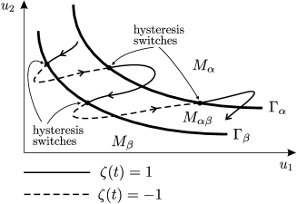
Let $\Gamma_{\alpha},\Gamma_{\beta}\subset\mathcal{U}$ be two disjoint smooth manifolds of codimension one without boundary (hysteresis “thresholds”). For simplicity, we assume that they are given by $\gamma_{\alpha}(u)=0$ and $\gamma_{\beta}(u)=0$ with $\nabla\gamma_{\alpha}(u)\neq 0$ and $\nabla\gamma_{\beta}(u)\neq 0$, respectively, where $\gamma_{\alpha}$ and $\gamma_{\beta}$ are $C^{\infty}$-smooth functions (in the general situation, atlases can be used).

Denote $M_{\alpha}=\{u\in\mathcal{U}:\gamma_{\alpha}(u)\leq 0\}$, $M_{\beta}=\{u\in\mathcal{U}:\gamma_{\beta}(u)\leq 0\}$, $M_{\alpha\beta}=\{u\in\mathcal{U}:\gamma_{\alpha}(u)>0,\ \gamma_{\beta}(u)>0\}$. Assume that $M_{\alpha}\cap\Gamma_{\beta}=\varnothing$ and $M_{\beta}\cap\Gamma_{\alpha}=\varnothing$ (Fig. 1).

Next, we introduce locally Hölder continuous functions (hysteresis “branches”)

$$W_{1}:D(W_{1})=M_{\alpha}\cup\overline{M}_{\alpha\beta}\to\mathcal{W},\qquad W_{-1}:D(W_{-1})=M_{\beta}\cup\overline{M}_{\alpha\beta}\to\mathcal{W}.$$

We fix $T>0$ and denote by $C_{r}[0,T)$ the space of functions continuous on the right in $[0,T)$. For any $\zeta_{0}\in\{1,-1\}$ (initial configuration) and $u_{0}\in C([0,T];\mathcal{U})$ (input), we introduce the configuration function

$$\zeta:\{1,-1\}\times C([0,T];\mathcal{U})\to C_{r}[0,T),\quad\zeta(t)=\zeta(\zeta_{0},u_{0})(t)$$

as follows. Let $X_{t}=\{s\in(0,t]:u_{0}(s)\in\Gamma_{\alpha}\cup\Gamma_{\beta}\}$. Then $\zeta(0)=1$ if $u_{0}(0)\in M_{\alpha}$, $\zeta(0)=-1$ if $u_{0}(0)\in M_{\beta}$, $\zeta(0)=\zeta_{0}$ if $u_{0}(0)\in M_{\alpha\beta}$; for $t\in(0,T]$, $\zeta(t)=\zeta(0)$ if $X_{t}=\varnothing$, $\zeta(t)=1$ if $X_{t}\neq\varnothing$ and $u_{0}(\max X_{t})\in\Gamma_{\alpha}$, $\zeta(t)=-1$ if $X_{t}\neq\varnothing$ and $u_{0}(\max X_{t})\in\Gamma_{\beta}$ (Fig. 1).

Refer to caption
Figure 1. Regions of different behavior of hysteresis $W$

Now we introduce the hysteresis operator $W:\{1,-1\}\times C([0,T];\mathcal{U})\to C_{r}[0,T)$ by the following rule (cf. [12, 18, 10]). For any initial configuration $\zeta_{0}\in\{1,-1\}$ and input $u_{0}\in C([0,T];\mathcal{U})$, the function $W(\zeta_{0},u_{0}):[0,T]\to\mathcal{W}$ (output) is given by

(1.3) $$W(\zeta_{0},u_{0})(t)=W_{\zeta(t)}(u_{0}(t)),$$

where $\zeta(t)$ is the configuration function defined above.

Assume that the initial configuration and the input function depend on spatial variable $x$. Denote them by $\xi_{0}(x)$ and $u(x,t)$, where $u(x,\cdot)\in C([0,T];\mathcal{U})$. Using (1.3) and treating $x$ as a parameter, we define the spatially distributed hysteresis

(1.4) $$W(\xi_{0}(x),u(x,\cdot))(t)=W_{\xi(x,t)}(u(x,t)),$$

where $\xi(x,t)=\zeta(\xi_{0}(x),u(x,\cdot))(t)$ is the spatial configuration.

1.2. Functional spaces.

Denote by $L_{q}(0,1)$, $q>1$, the standard Lebesgue space and by $W_{q}^{l}(0,1)$ with natural $l$ the standard Sobolev space. For a noninteger $l>0$, denote by $W_{q}^{l}(0,1)$ the Sobolev space with the norm

$$\|{\varphi}\|_{W_{q}^{[l]}(0,1)}+\left(\int_{0}^{1}dx\int_{0}^{1}\dfrac{|{\varphi}^{([l])}(x)-{\varphi}^{([l])}(y)|^{q}}{|x-y|^{1+q(l-[l])}}dy\right)^{1/q},$$

where $[l]$ is the integer part of $l$. Introduce the anisotropic Sobolev spaces $W_{q}^{2,1}(Q_{T})$ with the norm $\left(\int_{0}^{T}\|u(\cdot,t)\|_{W_{q}^{2}(0,1)}^{q}\,dt+\int_{0}^{T}\|u_{t}(\cdot,t)\|_{L_{q}(0,1)}^{q}\,dt\right)^{1/q}$ and the space $W_{\infty}^{0,1}(Q_{T})$ of $L_{\infty}(0,1)$-valued functions continuously differentiable on $[0,T]$ with the norm $\|v\|_{L_{\infty}(Q_{T})}+\|v_{t}\|_{L_{\infty}(Q_{T})}.$ Denote by $C^{\gamma}({\overline{Q}}_{T})$, $\gamma\in(0,1)$, the Hölder space.

For the vector-valued functions, we use the following notation. If, e.g., $u(x,t)\in\mathcal{U}$ and each component of $u$ belongs to $W_{q}^{2,1}(Q_{T})$, then we write $u\in W_{q}^{2,1}(Q_{T};\mathcal{U})$.

Throughout, we fix $q$ and $\gamma$ such that $q\in(3,\infty)$ and $\gamma\in(0,1-3/q).$ This implies that $u,u_{x}\in C^{\gamma}(\overline{Q}_{T};\mathcal{U})$ for $u\in W_{q}^{2,1}(Q_{T};\mathcal{U})$ (see Lemma 3.3 in [13, Chap. 2]).

To define the space of initial data, we use the fact that if $u\in W_{q}^{2,1}(Q_{T};\mathcal{U})$, then the trace $u|_{t=0}$ is well defined and belongs to $W_{q}^{2-2/q}((0,1);\mathcal{U})$ (see Lemma 2.4 in [13, Chap. 2]). We denote the norm in the latter space by $\|\cdot\|_{q}$. Moreover, one can define the space $W_{q,N}^{2-2/q}((0,1);\mathcal{U})$ as the subspace of functions from $W_{q}^{2-2/q}((0,1);\mathcal{U})$ with the zero Neumann boundary conditions.

We assume that ${\varphi}\in W_{q,N}^{2-2/q}((0,1);\mathcal{U})$ and $\psi\in L_{\infty}((0,1);\mathcal{V})$ in (1.2).

Definition 1.1.

A pair $(u,v)\in W_{q}^{2,1}(Q_{T};\mathcal{U})\times W_{\infty}^{0,1}(Q_{T};\mathcal{V})$ is a solution of problem (1.1), (1.2) if $W(\xi_{0},u)$ is measurable with respect to $(x,t)$ and (1.1), (1.2) hold.

1.3. Spatial transversality

We will deal with the case where $\xi_{0}(x)$ has one discontinuity point. Generalization to finitely many discontinuity points is straightforward.

Condition 1.1.
  1. (1)

    For some ${\overline{b}}\in(0,1)$, we have

    (1.5) $$\xi_{0}(x)=1\ (x\leq{\overline{b}}),\quad\xi_{0}(x)=-1\ (x>{\overline{b}}).$$
  2. (2)

    For $x\in[0,{\overline{b}}]$, we have ${\varphi}(x)\in M_{\alpha}\cup M_{\alpha\beta}$ or, equivalently, $\gamma_{\beta}({\varphi}(x))>0$.

  3. (3)

    For $x\in({\overline{b}},1]$, we have ${\varphi}(x)\in M_{\beta}\cup M_{\alpha\beta}$ or, equivalently, $\gamma_{\alpha}({\varphi}(x))>0$.

  4. (4)

    If $\gamma_{\alpha}({\varphi}({\overline{b}}))=0$, then $\dfrac{d}{dx}\gamma_{\alpha}({\varphi}(x))\Big{|}_{x=\overline{b}}>0$.

It follows from Condition 1.1 that the hysteresis in (1.4) at the initial moment equals $W_{1}({\varphi}(x))$ for $x\leq{\overline{b}}$ and $W_{2}({\varphi}(x))$ for $x>{\overline{b}}$. Items 2 and 3 in Condition 1.1 are necessary for the hysteresis to be well-defined at the initial moment, while item 4 is an essential assumption. We refer to item 4 as the spatial transversality and say that ${\varphi}(x)$ is transverse with respect to the spatial configuration $\xi_{0}(x)$. This means that if ${\varphi}(\overline{b})\in\Gamma_{\alpha}$, then the vector ${\varphi}^{\prime}(\overline{b})$ is transverse to the manifold $\Gamma_{\alpha}$ at this point.

Consider time-dependent functions $u(x,t)$ such that $u,u_{x}\in C(\overline{Q}_{T};\mathcal{U})$.

Definition 1.2.

We say that a function $u$ is transverse on $[0,T]$ $($with respect to a spatial configuration $\xi(x,t))$ if, for every fixed $t\in[0,T]$, either $\xi(\cdot,t)$ has no discontinuity points for $x\in(0,1)$, or it has one discontinuity point and the function $u(\cdot,t)$ is transverse with respect to the spatial configuration $\xi(\cdot,t)$.

Definition 1.3.

A function $u$ preserves spatial topology $($of a spatial configuration $\xi(x,t))$ on $[0,T]$ if there is $M>0$ such that, for $t\in[0,T]$, there is a continuous function $b(t)\in(0,1)$ such that $\xi(x,t)=1$ for $x\leq b(t)$ and $\xi(x,t)=-1$ for $x>b(t)$.

The solution from Definition 1.1 is called transverse (preserving spatial topology) if the function $u(x,t)$ is transverse (preserving spatial topology).

Remark 1.1.

The function $b(t)$ defining discontinuity of $\xi(x,t)$ plays a role of free boundary, which has much in common with free boundary in parabolic obstacle problems (see, e.g., [3, 15] and the references therein). However, in our case, the behavior of $b(t)$ is defined differently.

1.4. Assumptions on the right-hand side.

First, we assume the following.

Condition 1.2.

The functions $f(u,v,w)$ and $g(u,v,w)$ are locally Lipschitz continuous in $\mathbb{R}^{k}\times\mathbb{R}^{l}\times\mathbb{R}^{m}$.

Next, we formulate dissipativity conditions for $f$ and $g$.

In the following condition, we denote by $\mathcal{U}_{\mu}$, $\mu\geq 0$, closed parallelepipeds in $\mathcal{U}$ with the edges parallel to respective coordinate axes such that ${\varphi}(x)\in\mathcal{U}_{\mu}$ for all $x\in[0,1]$.

Condition 1.3.

There is a parallelepiped $\mathcal{U}_{0}$ and, for each sufficiently small $\mu>0$, there is a parallelepiped $\mathcal{U}_{\mu}$ and a locally Lipschitz continuous function $f_{\mu}(u,v)$ such that

  1. (1)

    $|f_{\mu}(u,v)|$ converges to 00 uniformly on compact sets in $\mathcal{U}\times\mathcal{V}$ as $\mu\to 0$,

  2. (2)

    At each point $u\in\partial{\mathcal{U}}_{0}\cap D(W_{\pm 1})$, $v\in\mathcal{V}$, the vector $f(u,v,W_{\pm 1}(u))+f_{\mu}(u,v)$ points strictly inside $\mathcal{U}_{0}$.

  3. (3)

    At each point $u\in\partial{\mathcal{U}}_{\mu}\cap D(W_{\pm 1})$, $v\in\mathcal{V}$, the vector $f(u,v,W_{\pm 1}(u_{\mu}))+f_{\mu}(u,v)$ points strictly inside $\mathcal{U}_{\mu}$ for all $u_{\mu}\in\mathcal{U}_{\mu}$.

To formulate the assumption on $g$, we fix ${\mathcal{U}}_{0}$ satisfying Condition 1.3 and set

(1.6) $${\mathcal{W}}_{0}=\bigcup_{j=\pm 1}\{W_{j}(u):u\in{\mathcal{U}}_{0}\}.$$
Condition 1.4.

For any $T_{0}>0$, there is a compact $\mathcal{V}_{0}=\mathcal{V}_{0}(T_{0},{\mathcal{U}}_{0})\subset\mathcal{V}$ such that $\psi(x)\in{\mathcal{V}}_{0}$ $((x\in(0,1))$ and the Cauchy problem

(1.7) $$v_{t}=g(u_{0}(x,t),v,w_{0}(x,t)),\quad v|_{t=0}=\psi(x)$$

has a solution $v\in W_{\infty}^{0,1}(Q_{T_{0}};{\mathbb{R}}^{l})$ satisfying $v(x,t)\in{\mathcal{V}}_{0}$ whenever

$$\begin{gathered}u_{0}\in L_{\infty}(Q_{T_{0}};{\mathcal{U}}),\quad w_{0}\in L_{\infty}(Q_{T_{0}};{\mathcal{W}}),\\ u_{0}(x,t)\in{\mathcal{U}}_{0},\quad w_{0}(x,t)\in{\mathcal{W}}_{0}\quad((x,t)\in Q_{T_{0}}).\end{gathered}$$
Remark 1.2.

It follows from [14, Theorem 1, p. 111] that system (1.7) has a unique solution $v\in W_{\infty}^{0,1}(Q_{T_{0}};{\mathbb{R}}^{l})$ for a sufficiently small $T_{0}>0$. Condition 1.4 additionally guarantees the absence of blow-up.

In particular, the uniform boundedness of $v$ holds if $|g(u,v,w)|\leq A(u,w)|v|+B(u,w)$, where $A(u,w)$ and $B(u,w)$ are bounded on compact sets (see Example 1.1). However, if $\mathcal{V}\neq\mathbb{R}^{l}$, one must additionally check that $v$ never leaves $\mathcal{V}$. To fulfill Condition 1.4, one could alternatively assume the existence of invariant parallelepiped for $g$ (similarly to Condition 1.3).

Example 1.1.

The hysteresis operator and the right-hand side in the present paper apply to a model describing a growth of a colony of bacteria (Salmonella typhimurium) on a petri plate (see [6, 7]). Let $u_{1}(x,t)$ and $u_{2}(x,t)$ denote the concentrations of diffusing buffer (pH level) and histidine (nutrient), respectively, while $v(x,t)$ denote the density of nondiffusing bacteria. These three unknown functions satisfy the following equations:

(1.8) $$\left\{\begin{aligned} u_{1t}&=D_{1}\Delta u_{1}-a_{1}W(\xi_{0},u)v,\\ u_{2t}&=D_{2}\Delta u_{2}-a_{2}W(\xi_{0},u)v,\\ v_{t}&=aW(\xi_{0},u)v,\\ \end{aligned}\right.$$

supplemented by initial and no-flux (Neumann) boundary conditions. In (1.8), $D_{1},D_{2},a,a_{1},a_{2}>0$ are given constants and $W(\xi_{0},u)$ is the hysteresis operator. In this example, we have $\mathcal{U}=\{u\in\mathbb{R}^{2}:u_{1},u_{2}\geq 0\}$, $\mathcal{V}=[0,\infty)$, $\mathcal{W}=[0,\infty)$. The hysteresis thresholds $\Gamma_{\alpha}$ and $\Gamma_{\beta}$ are the curves on the plane given by $\gamma_{\alpha}(u):=-u_{1}+a_{\alpha}/u_{2}+b_{\alpha}=0$ and $\gamma_{\beta}(u):=u_{1}-a_{\beta}/u_{2}-b_{\beta}=0$, respectively, where $a_{\alpha},a_{\beta},b_{\alpha},b_{\beta}>0$ are some constants (Fig. 1); the hysteresis “branches” are given by functions $W_{1}(u)$ $(>0)$ and $W_{-1}(u)$ $(\equiv 0)$.

2. Main results.

In what follows, we assume that Conditions 1.11.4 hold.

Theorem 2.1 (local existence).

There is a number $T>0$ such that

  1. (1)

    There is at least one solution of problem (1.1), (1.2) in $Q_{T};$

  2. (2)

    Any solution in $Q_{T}$ is transverse and preserves spatial topology.

Theorem 2.2 (continuation).

Let $(u,v)$ be a transverse topology preserving solution of problem (1.1), (1.2) in $Q_{T}$ for some $T>0$. Then it can be continued to an interval $[0,T_{max})$, where $T_{max}>T$ has the following properties. 1. For any $t_{0}<T_{max}$, the pair $(u,v)$ is a transverse solution of problem (1.1), (1.2) in $Q_{t_{0}}$. 2. Either $T_{max}=\infty$, or $T_{max}<\infty$ and $(u,v)$ is a solution in $Q_{T_{max}}$, but $u(\cdot,T_{max})$ is not transverse with respect to $\xi(\cdot,T_{max})$.

Theorem 2.3 (continuous dependence on initial data).

Assume the following.

  1. (1)

    There is a number $T>0$ such that problem (1.1), (1.2) with initial functions ${\varphi},\psi$ and initial configuration $\xi_{0}(x)$ defined by its discontinuity point ${\overline{b}}$ admits a unique transverse topology preserving solution $(u,v)$ in $Q_{s}$ for any $s\leq T$.

  2. (2)

    Let ${\varphi}_{n}\in W_{q,N}^{2-2/q}((0,1);\mathcal{U})$, $\psi_{n}\in L_{\infty}((0,1);\mathcal{V})$, $n=1,2,\dots$, be a sequence of other initial functions such that $\|{\varphi}-{\varphi}_{n}\|_{q}\to 0$, $\|\psi-\psi_{n}\|_{L_{q}((0,1);\mathcal{V})}\to 0$ as $n\to\infty$.

  3. (3)

    Let $\xi_{0n}(x)$, $n=1,2,\dots$, be a sequence of other initial configurations defined by their discontinuity points ${\overline{b}}_{n}$ similarly to (1.5) and ${\overline{b}}_{n}\to{\overline{b}}$ as $n\to\infty$.

Then, for all sufficiently large $n$, problem (1.1), (1.2) with initial data $({\varphi}_{n},\psi_{n},\xi_{0n})$ has at least one transverse topology preserving solution $(u_{n},v_{n})$. Each sequence of such solutions satisfies

$$\begin{gathered}\|u_{n}-u\|_{W_{q}^{2,1}(Q_{T};\mathcal{U})}\to 0,\quad\|b_{jn}-b_{j}\|_{C[0,T]}\to 0,\\ \sup\limits_{t\in[0,T]}\left(\|v_{n}(\cdot,t)-v(\cdot,t)\|_{L_{q}((0,1);{\mathcal{V}})}+\|v_{nt}(\cdot,t)-v_{t}(\cdot,t)\|_{L_{q}((0,1);{\mathcal{V}})}\right)\to 0\end{gathered}$$

as $n\to\infty,$ where $b(t)$ and $b_{n}(t)$ are the respective discontinuity points of the configuration functions $\xi(x,t)$ and $\xi_{n}(x,t)$.

Remark 2.1.

If one a priori knows that all $u_{n}$ are transverse on some interval $[0,T]\subset[0,T_{max})$, then one can prove that $u_{n}$ approximate $u$ on $[0,T]$ even if $u$ is not topology preserving on $[0,T]$.

Now we discuss the uniqueness of solutions. We strengthen the assumption about local Hölder continuity of $W_{\pm 1}$. Let $\mathcal{U}_{0}$ be the set from Condition 1.3.

Condition 2.1.

There are numbers $K>0$ and $\sigma\in[0,1)$ such that

$\displaystyle|W_{1}(u)-W_{1}(\hat{u})|$ $\displaystyle\leq\dfrac{K}{(\gamma_{\beta}(u))^{\sigma}+(\gamma_{\beta}(\hat{u}))^{\sigma}}|u-\hat{u}|\quad$ $\displaystyle\forall u,\hat{u}\in M_{\alpha}\cup\overline{M}_{\alpha\beta},$
$\displaystyle|W_{-1}(u)-W_{-1}(\hat{u})|$ $\displaystyle\leq\dfrac{K}{(\gamma_{\alpha}(u))^{\sigma}+(\gamma_{\alpha}(\hat{u}))^{\sigma}}|u-\hat{u}|\quad$ $\displaystyle\forall u,\hat{u}\in M_{\beta}\cup\overline{M}_{\alpha\beta}.$

We refer readers to [5] for the discussion about functions satisfying this condition.

Theorem 2.4 (uniqueness).

Assume additionally that Condition 2.1 holds. Let $(u,v)$ and $(\hat{u},\hat{v})$ be two transverse solutions of problem (1.1), (1.2) in $Q_{T}$ for some $T>0$. Then $(u,v)=(\hat{u},\hat{v})$.

3. Local existence, continuation
and continuous dependence of solutions on initial data

In this section, we prove Theorems 2.12.3. Throughout the section, we fix ${\mathcal{U}}_{0}$ satisfying Condition 1.3 and ${\mathcal{W}}_{0}$ given by (1.6). Next, we fix some $T_{0}\in(0,1]$ and then ${\mathcal{V}}_{0}$ satisfying Condition 1.4.

3.1. Preliminaries

The following result is straightforward.

Lemma 3.1.
  1. (1)

    Let $\lambda\in[0,1)$, $a\in C^{\lambda}[0,T]$, and $b(t)=\max\limits_{s\in[0,t]}a(s)$. Then $b\in C^{\lambda}[0,T]$ and $\|b\|_{C^{\lambda}[0,T]}\leq\|a\|_{C^{\lambda}[0,T]}.$

  2. (2)

    If $a_{j}\in C[0,T]$ and $b_{j}(t)=\max\limits_{s\in[0,t]}a_{j}(s)$, $j=1,2$, then $\|b_{1}-b_{2}\|_{C[0,T]}\leq\|a_{1}-a_{2}\|_{C[0,T]}.$

For some $T\leq T_{0}$, $u_{1}\in L_{\infty}(Q_{T};{\mathcal{U}})$, and $b_{1}\in C[0,T]$ such that $u_{1}(x,t)\in{\mathcal{U}}_{0}$ ($(x,t)\in Q_{T}$) and $b_{1}(t)\in[0,1)$ ($t\in[0,T]$), we define the function $w_{1}(x,t)$ by

(3.1) $$w_{1}(x,t)=\begin{cases}W_{1}(u_{1}(x,t)),&0\leq x\leq b_{1}(t),\\ W_{-1}(u_{1}(x,t)),&b_{1}(t)<x\leq 1;\end{cases}$$

here we assume $W_{\pm 1}(u_{1})$ to be extended to ${\mathcal{U}}_{0}$ without loss of regularity.

Lemma 3.2.

Let $u_{1},b_{1}$ be functions with the above properties, and let $\hat{u}_{1},\hat{b}_{1}$ be functions with the same properties. Let $w_{1}$ be defined by (3.1) and $\hat{w}_{1}$ by (3.1) with $\hat{u}_{1}$ and $\hat{b}_{1}$ instead of $u_{1}$ and $b_{1}$, respectively. Then, for any $p\in[1,\infty)$,

$$\|w_{1}-\hat{w}_{1}\|_{L_{p}(Q_{T};{\mathcal{W}})}\leq c_{0}\left(T^{1/p}\|u_{1}-\hat{u}_{1}\|_{L_{\infty}(Q_{T};{\mathcal{U}})}^{\sigma_{0}}+\|b_{1}-\hat{b}_{1}\|_{L_{1}(0,T)}^{1/p}\right),$$

where $\sigma_{0}$ is a Hölder exponent for $W_{\pm 1}(u_{1})$ and $c_{0}>0$ depends on ${\mathcal{U}}_{0}$ and $p$, but does not depend on $u_{1},b_{1},T$.

Proof.

We fix some $t\in[0,T]$ and assume that $b_{1}(t)\leq\hat{b}_{1}(t)$ for this $t$. Then, using (3.1) and omitting the arguments of the integrands, we have

$\displaystyle\int\limits_{0}^{1}|w_{1}-\hat{w}_{1}|^{p}\,dx$ $\displaystyle=\int\limits_{0}^{b_{1}(t)}|W_{1}(u_{1})-W_{1}(\hat{u}_{1})|^{p}\,dx+\int\limits_{\hat{b}_{1}(t)}^{1}|W_{-1}(u_{1})-W_{-1}(\hat{u}_{1})|^{p}\,dx$
$\displaystyle+\int\limits_{b_{1}(t)}^{\hat{b}_{1}(t)}|W_{-1}(u_{1})-W_{1}(\hat{u}_{1})|^{p}\,dx.$

Using the Hölder continuity and the boundedness of $W_{\pm 1}(u_{1})$ for $u_{1}\in{\mathcal{U}}_{0}$ and integrating with respect to $t$ from 00 to $T$, we complete the proof. ∎

Now we introduce sets that “measure” the spatial transversality. Denote by $E_{m}$, $m\in\mathbb{N}$, the set of triples $({\varphi},\psi,\xi_{0})$ such that ${\varphi}\in W_{q,N}^{2-2/q}((0,1);{\mathcal{U}})$, $\psi\in L_{\infty}((0,1);{\mathcal{V}})$, $\xi_{0}(x)$ is of the form (1.5), and the following hold:

  1. (1)

    ${\overline{b}}\in[1/m,1-1/m]$,

  2. (2)

    $\gamma_{\beta}({\varphi}(x))\geq 1/m^{2}$ for $x\in[0,{\overline{b}}]$,

  3. (3)

    $\gamma_{\alpha}({\varphi}(x))\geq 1/m^{2}$ for $x\in[{\overline{b}}+1/m,1]$,

  4. (4)

    if $x\in[{\overline{b}},{\overline{b}}+1/m]$ and $\gamma_{\alpha}({\varphi}(x))\in[0,1/m^{2}]$, then $\dfrac{d}{dx}\gamma_{\alpha}({\varphi}(x))\geq 1/m$,

  5. (5)

    $\|{\varphi}\|_{q}\leq m$ and $\|\psi\|_{L_{\infty}((0,1);{\mathcal{V}})}\leq m$.

It is easy to check that $E_{m}\subset E_{m+1}$. Moreover, one can show (Lemma 2.25 in [4]) that the union of all sets $E_{m}$ coincides with the set of all data satisfying Condition 1.1. From now on, we fix $m\in{\mathbb{N}}$ such that $({\varphi},\psi,\xi_{0})\in E_{m}$.

The next lemma follows from the implicit function theorem and Lemma 3.1.

Lemma 3.3.

Let $\lambda\in(0,1)$, $u_{1},u_{1x}\in C^{\lambda}({\overline{Q}}_{T_{0}};{\mathcal{U}})$,

$$\|u_{1}\|_{C^{\lambda}({\overline{Q}}_{T_{0}};{\mathcal{U}})}+\|u_{1x}\|_{C^{\lambda}({\overline{Q}}_{T_{0}};{\mathcal{U}})}\leq c$$

for some $c>0$, $u_{1}|_{t=0}=\varphi(x)$, and $(\varphi,\psi,\xi_{0})\in E_{m}$. Then there is $T_{1}=T_{1}(m,\lambda,c)\leq T_{0}$ and a natural number $N_{1}=N_{1}(m,\lambda,c)\geq m$ which do not depend on $u,{\varphi},\xi_{0}$ such that the following is true for any $t\in[0,T_{1}]$.

  1. (1)

    The equation $\gamma_{\alpha}(u_{1}(x,t))=0$ for $x\in[{\overline{b}},1]$ has no more than one root. If this root exists, we denote it by $a_{1}(t);$ otherwise, we set $a_{1}(t)={\overline{b}}$. One has $a_{1}(t)\in[{\overline{b}},{\overline{b}}+1/N_{1}]$, $a_{1}\in C^{\lambda}[0,T_{1}]$.

  2. (2)

    The hysteresis ${\mathcal{H}}(\xi_{0},u_{1})$ and its configuration function $\xi_{1}(x,t)$ have exactly one discontinuity point $b_{1}(t);$ moreover, $b_{1}(t)=\max\limits_{s\in[0,t]}a_{1}(s)$, $b_{1}\in C^{\lambda}[0,T_{1}]$.

3.2. Auxiliary problem

Consider functions $u_{1}\in L_{\infty}(Q_{T};{\mathcal{U}})$ and $w_{1}\in L_{\infty}(Q_{T};{\mathcal{W}})$ such that

$$u_{1}(x,t)\in{\mathcal{U}}_{0},\quad w_{1}(x,t)\in{\mathcal{W}}_{0}\quad((x,t)\in Q_{T})$$

for some $T>0$. Define the functions

(3.2) $$f_{1}(u,v,x,t)=f(u,v,w_{1}(x,t)),\quad g_{1}(v,x,t)=g(u_{1}(x,t),v,w_{1}(x,t)).$$

Consider the auxiliary problem

(3.3) $$\left\{\begin{aligned} &u_{t}=Du_{xx}+f_{1}(u,v,x,t),\\ &v_{t}=g_{1}(v,x,t)\\ &u|_{t=0}={\varphi}(x),\quad v|_{t=0}=\psi(x),\quad u_{x}|_{x=0}=u_{x}|_{x=1}=0.\end{aligned}\right.$$

Set $f_{U}=\sup f(u,v,w)$ and $g_{U}=\sup g(u,v,w)$, where $(u,v,w)\in{\mathcal{U}}_{0}\times{\mathcal{V}}_{0}\times{\mathcal{W}}_{0}$.

The next result follows from the standard estimates for solutions of linear parabolic equations [13], from Conditions 1.21.4 combined with the principle of invariant rectangles [16], and from Lemma 3.3.

Lemma 3.4.
  1. (1)

    For any $T\leq T_{0}$, problem (3.3) has a unique solution $(u,v)\in W_{q}^{2,1}(Q_{T};{\mathcal{U}})\times W_{\infty}^{0,1}(Q_{T};{\mathcal{V}})$ and

    $$\displaystyle u(x,t)\in{\mathcal{U}}_{0},\quad v(x,t)\in{\mathcal{V}}_{0}\quad((x,t)\in Q_{T}),$$
    $$\displaystyle\|u\|_{W_{q}^{2,1}(Q_{T};{\mathcal{U}})}+\max_{t\in[0,T]}\|u(\cdot,t)\|_{q}\leq c_{1}(\|{\varphi}\|_{q}+f_{U}),$$
    $$\displaystyle\|v\|_{W_{\infty}^{0,1}(Q_{T};{\mathcal{V}})}\leq\|\psi\|_{L_{\infty}((0,1);{\mathcal{V}})}+2g_{U},$$
    (3.4) $$\displaystyle\|u\|_{C^{\gamma}({\overline{Q}}_{T};{\mathcal{U}})}+\|u_{x}\|_{C^{\gamma}({\overline{Q}}_{T};{\mathcal{U}})}\leq c_{2}(\|{\varphi}\|_{q}+f_{U}),$$

    where $c_{1},c_{2}>0$ depend only on $T_{0}$.

  2. (2)

    If $u_{n},v_{n}$, $n=1,2,\dots$, are solutions of problem (3.2), (3.3) with $u_{1},w_{1}$ replaced by $u_{1n},w_{1n}$ $($with the same properties$)$ and

    $$\|u_{1n}-u_{1}\|_{L_{\infty}(Q_{T};{\mathcal{U}})}+\|w_{1n}-w_{1}\|_{L_{q}(Q_{T};{\mathcal{W}})}\to 0,\quad n\to\infty,$$

    then

    $$\|u_{n}-u\|_{W_{q}^{2,1}(Q_{T};{\mathcal{U}})}+\|v_{n}-v\|_{W_{q}^{0,1}(Q_{T};{\mathcal{V}})}\to 0,\quad n\to\infty.$$
  3. (3)

    There is $T_{2}=T_{2}(m)\leq T_{0}$ and a natural number $N_{2}=N_{2}(m)\geq m$ such that, for any $t\in[0,T_{2}]$, conclusions (1) and (2) from Lemma 3.3 hold for $u(x,t)$, for the corresponding “root” function $a(t)$, for the configuration function $\xi(x,t)$ of the hysteresis ${\mathcal{H}}(\xi_{0},u)$, for its discontinuity point $b(t)$, and for $T_{2},N_{2}$ instead of $T_{1},N_{1}$. Furthermore, $(u(\cdot,t),v(\cdot,t),\xi(\cdot,t))\in E_{N_{2}}$.

3.3. Local existence: proof of Theorem 2.1

1. Let us prove the first assertion.

1.1. Fix $\lambda$ in Lemma 3.3 such that $\lambda\in(0,\gamma)$. Fix $c_{2}$ from Lemma 3.4. Set $c=c_{\lambda,\gamma}c_{2}(m+f_{U})$, where $c_{\lambda,\gamma}>0$ is the embedding constant such that $\|u\|_{C^{\lambda}({\overline{Q}}_{T};{\mathcal{U}})}\leq c_{\lambda,\gamma}\|u\|_{C^{\gamma}({\overline{Q}}_{T};{\mathcal{U}})}$. Set $T=\min(T_{1},T_{2})$, where $T_{1},T_{2}$ are defined in Lemmas 3.3, 3.4.

Let $R^{\lambda}({\overline{Q}}_{T})$ be the set of functions $u(x,t)$ such that $u|_{t=0}={\varphi}(x)$,

$$\displaystyle u,u_{x}\in C^{\lambda}({\overline{Q}}_{T};{\mathcal{U}}),\quad u(x,t)\in{\mathcal{U}}_{0}\quad((x,t)\in Q_{T}),$$
(3.5) $$\displaystyle\|u\|_{C^{\lambda}({\overline{Q}}_{T};{\mathcal{U}})}+\|u_{x}\|_{C^{\lambda}({\overline{Q}}_{T};{\mathcal{U}})}\leq c.$$

The set $R^{\lambda}({\overline{Q}}_{T})$ is a closed convex subset of the Banach space endowed with the norm given by the left-hand side in (3.5). Similarly, we define $R^{\gamma}({\overline{Q}}_{T})$.

1.2. We construct a map ${\mathcal{R}}:R^{\lambda}({\overline{Q}}_{T})\to R^{\gamma}({\overline{Q}}_{T})$. Take any $u_{1}\in R^{\lambda}({\overline{Q}}_{T})$ and define $a_{1}(t)$ and $b_{1}(t)$ according to Lemma 3.3. Then define $w_{1}(x,t)$ by (3.1) and, using this $w_{1}$, define $f_{1},g_{1}$ by (3.2). Finally apply Lemma 3.4 and obtain a solution $(u,v)$ of auxiliary problem (3.3). We now define ${\mathcal{R}}:u_{1}\mapsto u$.

The operator ${\mathcal{R}}$ is continuous. Indeed, it is not difficult to check that the mapping $u_{1}\mapsto a_{1}$ is continuous from $R^{\lambda}({\overline{Q}}_{T})$ to $C[0,T]$. Thus, the continuity of ${\mathcal{R}}$ follows by consecutively applying Lemmas 3.1 (part 2), 3.2, 3.4 (part 2), and the continuity of the embedding $W_{q}^{2,1}(Q_{T};{\mathcal{V}})\subset R^{\gamma}({\overline{Q}}_{T})$.

Furthermore, due to (3.4) and the choice of $c$, the operator ${\mathcal{R}}$ maps $R^{\lambda}({\overline{Q}}_{T})$ into itself. As an operator acting from $R^{\lambda}({\overline{Q}}_{T})$ into itself, it is compact due to (3.4) and the compactness of the embedding $R^{\gamma}({\overline{Q}}_{T})\subset R^{\lambda}({\overline{Q}}_{T})$. Therefore, applying the Schauder fixed-point, we conclude the proof of the first assertion of the theorem. Note that ${\mathcal{R}}$ is not Lipschitz continuous (mind the exponent $1/p$ in (3.2)). Hence, the contraction principle does not apply. We prove uniqueness separately in Sec. 4.

2. The second assertion follows by applying the principle of invariant rectangles (see [16]) and Lemma 3.4.

3.4. Continuation: proof of Theorem 2.2

Theorem 2.2 follows from part 3 of Lemma 3.4 and from the following fact (see Lemma 2.25 in [4]). Assume (1) $({\varphi}_{m},\psi_{m},\xi_{m})\in E_{m}\setminus E_{m-1}$, $m=2,3,\dots$; (2) $\|{\varphi}_{m}-{\varphi}\|_{q}\to 0$ and $\|\psi_{m}-\psi\|_{L_{\infty}((0,1);{\mathcal{V}})}\to 0$ as $m\to\infty$ for some ${\varphi}\in W_{q}^{2-2/q}((0,1);\mathcal{U})$ and $\psi\in L_{\infty}((0,1);{\mathcal{V}})$; (3) ${\overline{b}}_{m}-{\overline{b}}\to 0$ as $m\to\infty$ for some ${\overline{b}}\in[0,1]$. Then ${\overline{b}}\in\{0,1\}$ or ${\varphi}(x)$ is not transverse with respect to $\xi_{0}(x)$, where $\xi_{0}(x)$ is given by (1.5).

3.5. Continuous dependence on initial data: proof of Theorem 2.3

1. It suffices to prove the theorem for a sufficiently small time interval. Since $({\varphi},\psi,\xi_{0})\in E_{m}$, it is easy to show that there is $n_{1}=n_{1}(m)>0$ such that $({\varphi},\psi,\xi_{0}),({\varphi}_{n},\psi_{n},\xi_{0n})\in E_{m+1}$ for all $n\geq n_{1}(m)$. Hence, by Theorem 2.1, there is $T\in(0,1]$ for which problem (1.1), (1.2) has transverse topology preserving solutions $(u,v)$ and $(u_{n},v_{n})$ with the corresponding initial data. Moreover, any solution of problem (1.1), (1.2) in $Q_{T}$ is transverse and preserves topology.

We introduce the functions $a(t)$ and $a_{n}(t)$ corresponding to $u$ and $u_{n}$ as described in part 3 of Lemma 3.4. Then the discontinuity points of the corresponding configuration functions $\xi(x,t)$, $\xi_{n}(x,t)$ are given by $b(t)=\max\limits_{s\in[0,t]}a(s)$ and $b_{n}(t)=\max\limits_{s\in[0,t]}a_{n}(s)$.

2. Assume that there is $\varepsilon>0$ such that

(3.6) $$\|u_{n}-u\|_{W_{q}^{2,1}(Q_{T};{\mathcal{U}})}\geq\varepsilon,\quad n=1,2,\dots,$$

for some subsequence of $u_{n}$, which we denote $u_{n}$ again. Theorem 2.1 implies that $u_{n}$ and $a_{n}$ are uniformly bounded in $W_{q}^{2,1}(Q_{T};{\mathcal{U}})$ and $C^{\gamma}[0,T]$, respectively. Hence, we can choose subsequences of $u_{n}$ and $a_{n}$ (which we denote $u_{n}$ and $a_{n}$ again) such that

(3.7) $$\displaystyle\|u_{n}-\hat{u}\|_{C^{\gamma}({\overline{Q}}_{T};{\mathcal{U}})}\to 0,\quad\|(u_{n})_{x}-\hat{u}_{x}\|_{C^{\gamma}({\overline{Q}}_{T};{\mathcal{U}})}\to 0,\quad n\to\infty,$$
(3.8) $$\displaystyle\|a_{n}-\hat{a}\|_{C[0,T]}\to 0,\quad n\to\infty$$

for some function $\hat{u}\in C^{\gamma}({\overline{Q}}_{T};{\mathcal{U}})$ with $\hat{u}_{x}\in C^{\gamma}({\overline{Q}}_{T};{\mathcal{U}})$ and some $\hat{a}\in C[0,T]$.

Set $\hat{b}(t)=\max\limits_{s\in[0,t]}\hat{a}(s)$. Due to (3.7), (3.8), and Lemma 3.1, we have

(3.9) $$\displaystyle\|b_{n}-\hat{b}\|_{C[0,T]}\to 0,\quad n\to\infty,$$
(3.10) $$\displaystyle W(\xi_{0}(x),\hat{u}(x,\cdot))(t)=\begin{cases}W_{1}(\hat{u}(x,t)),&0\leq x\leq\hat{b}(t),\\ W_{2}(\hat{u}(x,t)),&\hat{b}(t)<x\leq 1.\end{cases}$$

3. Now we show that

(3.11) $$\sup\limits_{t\in[0,T]}\left(\|v_{n}(\cdot,t)-\hat{v}(\cdot,t)\|_{L_{q}((0,1);{\mathcal{V}})}+\|v_{nt}(\cdot,t)-\hat{v}_{t}(\cdot,t)\|_{L_{q}((0,1);{\mathcal{V}})}\right)\to 0,\quad n\to\infty,$$

for some $\hat{v}$. Take an arbitrary $\delta>0$. It follows from the assumptions of the theorem, from (3.7), (3.9), (3.10), and from Lemma 3.2 that

(3.12) $$\begin{gathered}\|\psi_{n}-\psi_{k}\|_{L_{q}((0,1);{\mathcal{V}})}\leq\delta,\quad\|u_{n}(\cdot,t)-u_{k}(\cdot,t)\|_{L_{q}((0,1);{\mathcal{U}})}\leq\delta,\\ \|W(\xi_{n},u_{n})(t)-W(\xi_{k},u_{k})(t)\|_{L_{q}((0,1);{\mathcal{W}})}\leq\delta,\end{gathered}$$

provided $n,k$ are large enough. Estimates (3.12), the second equation in (1.1), and the local Lipschitz continuity of $g$ yield

$$\|v_{n}(\cdot,t)-v_{k}(\cdot,t)\|_{L_{q}((0,1);{\mathcal{V}})}\leq(1+2L)\delta+L\int\limits_{0}^{t}\|v_{n}(\cdot,s)-v_{k}(\cdot,s)\|_{L_{q}((0,1);{\mathcal{V}})}\,ds,$$

where $L>0$ does not depend on $n,k$. Hence, by Gronwall’s inequality,

(3.13) $$\|v_{n}(\cdot,t)-v_{k}(\cdot,t)\|_{L_{q}((0,1);{\mathcal{V}})}\leq k_{1}\delta,$$

where $k_{1}>0$ does not depend $\delta,n,k,$ and $t\in[0,T]$. A similar inequality for the time derivative of $v_{n}$ follows from (3.12), (3.13), and from the second equation in (1.1). Since $\delta>0$ is arbitrary, (3.11) does hold.

Now consider (1.1), (1.2) with the subsequence ${\varphi}_{n},\psi_{n},\xi_{0n},u_{n},v_{n}$ and pass to the limit as $n\to\infty$. Due to the uniqueness assumption, $(u,v)=(\hat{u},\hat{v})$. Therefore, (3.6) is not true and we have the convergence for the whole sequence $(u_{n},v_{n})$.

4. Uniqueness of solutions

In this section, we prove Theorem 2.4. For the clarity of exposition, we restrict ourselves to the case where initial data satisfy the equality $\gamma_{\alpha}(\varphi({\overline{b}}))=0$ in addition to Condition 1.1. (The case $\gamma_{\alpha}(\varphi({\overline{b}}))\neq 0$ can be treated easily because then the hysteresis $W(\xi_{0},u)$ remains constant on some time interval.)

Set

$${\overline{\varphi}}:=\frac{1}{2}\frac{d}{dx}\gamma_{\alpha}({\varphi}(x))|_{x={\overline{b}}}\ (>0).$$

We fix $T_{1}$ such that the conclusions of Lemma 3.3 are true for the $u$, ${\hat{u}}$ on $(0,T_{1})$. Let $a(t)$, $b(t)$, $\hat{a}(t)$, $\hat{b}(t)$ be the functions defined in Lemma 3.3 for $u$ and ${\hat{u}}$, respectively. We fix $T\in(0,T_{1})$ and $\delta>0$ such that the following hold for $t\in[0,T]$ $:$

(4.1) $$\displaystyle\frac{d}{dx}\gamma_{\alpha}(u(x,t))\geq{\overline{\varphi}},\quad x\in[{\overline{b}}-\delta,{\overline{b}}+\delta],$$
(4.2) $$\displaystyle\gamma_{\beta}(u(x,t))<0,\quad x\in[0,b(t)],$$

and the analogous inequalities hold for ${\hat{u}}$.

Due to (4.1) and (4.2), we have

(4.3) $\displaystyle W(\xi_{0}(x),u(x,\cdot)(t)$ $\displaystyle=\begin{cases}W_{1}(u(x,t)),&0\leq x\leq b(t),\\ W_{-1}(u(x,t)),&b(t)<x\leq 1,\end{cases}$
$\displaystyle W(\xi_{0}(x),\hat{u}(x,\cdot)(t)$ $\displaystyle=\begin{cases}W_{1}(\hat{u}(x,t)),&0\leq x\leq\hat{b}(t),\\ W_{-1}(\hat{u}(x,t)),&\hat{b}(t)<x\leq 1.\end{cases}$

Let us now prove Theorem 2.4.

1. Denote $w=u-{\hat{u}}$, $z=v-{\hat{v}}$. The functions $w$, $z$ satisfy the equations

(4.4) $$\left\{\begin{aligned} &w_{t}=w_{xx}+h_{w}(x,t),\\ &z_{t}=h_{z}(x,t),\end{aligned}\right.$$

and the zero boundary and initial conditions, where

$\displaystyle h_{w}(x,t)$ $\displaystyle=f(u,v,W(u))-f({\hat{u}},{\hat{v}},W({\hat{u}})),$
$\displaystyle h_{z}(x,t)$ $\displaystyle=g(u,v,W(u))-g({\hat{u}},{\hat{v}},W({\hat{u}})).$

Obviously, $h_{w,z}\in L_{\infty}(Q_{T})$. The function $w$ can be represented via the Green function $G(x,y,t,s)$ of the heat equation with the Neumann boundary conditions:

$$w(x,t)=\int\limits_{0}^{t}\int\limits_{0}^{1}G(x,y,t,s)h_{w}(y,s)\,dyds.$$

Therefore, using the estimate $|G(x,y,t,s)|\leq\dfrac{k_{1}}{\sqrt{t-s}}$, $0<s<t$, with $k_{1}>0$ not depending on $(x,t)\in Q_{T}$ (see, e.g., [9]), we obtain

(4.5) $$|w(x,t)|\leq k_{1}\int\limits_{0}^{t}\dfrac{ds}{\sqrt{t-s}}\int\limits_{0}^{1}|h_{w}(y,s)|\,dy.$$

Set $Z(t)=\int_{0}^{1}|h_{z}(y,t)|dy$. Due to the second equation in (4.4),

(4.6) $$Z(t)\leq\int\limits_{0}^{t}\int\limits_{0}^{1}|h_{z}(y,s)|dyds.$$

2. Now we prove that, for some $k_{2}>0$,

(4.7) $$\int\limits_{0}^{1}|h_{w,z}(y,s)|dy\leq k_{2}(\|w\|_{C({\overline{Q}}_{T})}+\|Z\|_{L_{\infty}(0,T)}),\quad s\in(0,T).$$

Let us prove this inequality for the function $h_{w}$, assuming that $b(s)<\hat{b}(s)$. (The cases of $h_{z}$ and $b(s)\geq\hat{b}(s)$ are treated analogously.) Since $f$ is locally Lipschitz,

(4.8) $$\int\limits_{0}^{1}|h_{w}(y,s)|dy\leq k_{3}\int\limits_{0}^{1}(|w(y,s)|+|z(y,s)|+|W(u(y,s))-W({\hat{u}}(y,s))|)\leq\\ \leq k_{3}\left(\|w\|_{C({\overline{Q}}_{T})}+\|Z\|_{L_{\infty}(0,T)}+\int\limits_{0}^{1}|W(u(y,s))-W({\hat{u}}(y,s))|dy\right),$$

where $k_{3}>0$ and the constants $k_{4},k_{5},\ldots>0$ below do not depend on $s\in[0,T]$.

Denote $\theta(y,s)=W(u(y,s))-W({\hat{u}}(y,s))$. Due to (4.3), we have

$$\theta(y,s)=\begin{cases}W_{1}(u)-W_{1}(\hat{u}),&0<y<b(s),\\ W_{-1}(u)-W_{1}(\hat{u}),&b(s)<y<\hat{b}(s),\\ W_{-1}(u)-W_{-1}(\hat{u}),&\hat{b}(s)<y<1.\end{cases}$$

2.1. Inequality (4.2) implies that $\gamma_{\beta}(u(y,s))<0$,$\gamma_{\beta}(\hat{u}(y,s))<0$ on the closed set $\{(y,s):y\in[0,b(s)],\ s\in[0,T]\}$. Hence, the values $\gamma_{\beta}(u(y,s))$ and $\gamma_{\beta}(\hat{u}(y,s))$ are separated from 0. Therefore, using Condition 2.1, we obtain

(4.9) $$\int\limits_{0}^{b(s)}|\theta(y,s)|\,dy\leq k_{4}\int\limits_{0}^{b(s)}|u(y,s)-\hat{u}(y,s)|\,dy\leq k_{4}\|w\|_{C({\overline{Q}}_{T})}.$$

2.2. Boundedness of $W_{1}(\hat{u})$ and $W_{-1}(u)$ for $(y,s)\in{\overline{Q}}_{T}$ and Lemma 3.1 imply

(4.10) $$\int\limits_{b(s)}^{\hat{b}(s)}|\theta(y,s)|\,dy\leq k_{5}\int\limits_{b(s)}^{\hat{b}(s)}\,dy\leq k_{5}\|b-\hat{b}\|_{C[0,T]}\leq k_{5}\|a-\hat{a}\|_{C[0,T]}.$$

Using (4.1), we obtain for any $t\in[0,T]$ the inequalities

(4.11) $\displaystyle|a(t)-\hat{a}(t)|$ $\displaystyle\leq\dfrac{1}{{\overline{\varphi}}}|\gamma_{\alpha}(u(a(t),t))-\gamma_{\alpha}(\hat{u}(a(t),t))|\leq$
$\displaystyle\leq\dfrac{L_{\alpha}}{{\overline{\varphi}}}|u(a(t),t)-\hat{u}(a(t),t)|\leq\dfrac{L_{\alpha}}{{\overline{\varphi}}}\|u-\hat{u}\|_{C({\overline{Q}}_{T})},$

where $L_{\alpha}>0$ is a respective Lipschitz constant for $\gamma_{\alpha}(u)$ and hence does not depend on $T\in(0,T_{1})$. Inequalities (4.10) and (4.11) yield

(4.12) $$\int\limits_{b(s)}^{\hat{b}(s)}|\theta(y,s)|\,dy\leq k_{6}\|w\|_{C({\overline{Q}}_{T})}.$$

2.3. Let $y\in[\hat{b}(s),{\overline{b}}+\delta]$. Inequality (4.1) and the mean-value theorem imply

$$\begin{gathered}\gamma_{\alpha}({\hat{u}}(y,s))=\gamma_{\alpha}({\hat{u}}(y,s))-\gamma_{\alpha}({\hat{u}}(\hat{a}(s),s))\geq(y-\hat{a}(s)){\overline{\varphi}}\geq(y-\hat{b}(s)){\overline{\varphi}},\\ |\gamma_{\alpha}(u(y,s))|\geq(y-b(s)){\overline{\varphi}}.\end{gathered}$$

Taking into account these two inequalities and using Condition 2.1, we obtain

(4.13) $$\int\limits_{\hat{b}(s)}^{{\overline{b}}+\delta}|\theta(y,s)|\,dy\leq k_{7}\int\limits_{\hat{b}(s)}^{{\overline{b}}+\delta}\dfrac{|u(y,s)-\hat{u}(y,s)|}{(y-\hat{b}(s))^{\sigma}}\,dy\leq k_{8}\|w\|_{C({\overline{Q}}_{T})}.$$

2.4. Similarly to item 2.1, we conclude that

(4.14) $$\int\limits_{{\overline{b}}+\delta}^{1}|\theta(y,s)|\,dy\leq k_{9}\|w\|_{C({\overline{Q}}_{T})}.$$

Finally, (4.8)–(4.14) imply (4.7).

3. Combining estimates (4.5)–(4.7), we obtain

$\displaystyle|w(x,t)|$ $\displaystyle\leq k_{10}(\|w\|_{C({\overline{Q}}_{T})}+\|Z\|_{L_{\infty}(0,T)})\int\limits_{0}^{t}\dfrac{ds}{\sqrt{t-s}}$
$\displaystyle=2k_{10}T^{1/2}(\|w\|_{C({\overline{Q}}_{T})}+\|Z\|_{L_{\infty}(0,T)}),$
$\displaystyle Z(t)$ $\displaystyle\leq k_{2}T(\|w\|_{C({\overline{Q}}_{T})}+\|Z\|_{L_{\infty}(0,T)}).$

Taking the supremum with respect to $t\in(0,T)$, we see that

$$\|w\|_{C({\overline{Q}}_{T})}+\|Z\|_{L_{\infty}(0,T)}\leq(2k_{10}T^{1/2}+k_{2}T)(\|w\|_{C({\overline{Q}}_{T})}+\|Z\|_{L_{\infty}(0,T)}).$$

Thus, $w=0$ and $z=0$, provided that $T>0$ is small enough. ∎

References

  • [1] T. Aiki, J. Kopfová. A Mathematical Model for Bacterial Growth Described by a Hysteresis Operator. Recent advances in nonlinear analysis – Proceedings of the International Conference on Nonlinear Analysis. Hsinchu, Taiwan, 2006.
  • [2] H. W. Alt. On the thermostat problem. Control Cyb., 14, 171–193 (1985).
  • [3] D. Apushinskaya, H.Shahgholian, N.N.Uraltseva. On the Lipschitz property of the free boundary in a parabolic problem with an obstacle. St. Petersburg Math. J., 15, no. 3, 375–391 (2004).
  • [4] P. Gurevich, R. Shamin, S. Tikhomirov. Reaction-Diffusion Equations with Spatially Distributed Hysteresis. SIAM J. Math. Anal. 45, no. 3, 1328-1355 (2013).
  • [5] P. Gurevich, S. Tikhomirov. Uniqueness of transverse solutions for reaction-diffusion equations with spatially distributed hysteresis. Nonlinear Analysis Series A: Theory, Methods and Applications, 75, 6610–6619 (2012).
  • [6] F. C. Hoppensteadt, W. Jäger. Lecture Notes in Biomathematics 38, 68–81 (1980).
  • [7] F. C. Hoppensteadt, W. Jäger, C. Poppe. Modelling of Patterns in Space and Time, Lecture Notes in Biomath. 55 (Springer), 123–134 (1984).
  • [8] A. M. Il’in, B. A. Markov. A nonlinear diffusion equation and Liesegang rings. Doklady Mathematics, 84, No. 2, 730–733 (2011).
  • [9] S. D. Ivasi$\check{s}$en Green’s matrices of boundary value problems for Petrovski parabolic systems of general form, II, Mat. Sb., 114(156), No. 4, 523–565 (1981); English transl. in Math. USSR Sbornik, 42 461–489 (1982).
  • [10] O. Klein. Representation of hysteresis operators acting on vector-valued monotaffine functions, Adv. Math. Sci. Appl., 22, 471–500 (2012).
  • [11] J. Kopfová. Hysteresis in biological models. Proceedings of the conference “International Workshop on Multi-rate processess and hysteresis”, Journal of Physics, Conference Series, 55, 130–134 (2006).
  • [12] M. A. Krasnosel’skii, A. V. Pokrovskii. Systems with Hysteresis. Springer-Verlag. Berlin–Heidelberg–New York (1989).
  • [13] O. A. Ladyzhenskaya, V. A. Solonnikov, N. N. Uraltseva. Linear and Quasilinear Equations of Parabolic Type. Nauka, Moscow, 1967.
  • [14] F. Rothe. Global Solutions of Reaction-Diffusion Systems. Lecture Notes in Mathematics, 1072. Springer-Verlag, Berlin (1984).
  • [15] H. Shahgholian, N. Uraltseva, G. S. Weiss. A parabolic two-phase obstacle-like equation. Advances in Mathematics, 221, 861–881 (2009).
  • [16] J. Smoller. Shock Waves and Reaction-Diffusion Equations. Second edition. Grundlehren der Mathematischen Wissenschaften [Fundamental Principles of Mathematical Sciences], 258. Springer-Verlag, New York (1994).
  • [17] A. Visintin. Evolution problems with hysteresis in the source term. SIAM J. Math. Anal, 17, 1113–1138 (1986).
  • [18] A. Visintin. Differential Models of Hysteresis. Springer-Verlag. Berlin — Heidelberg (1994).

Authors’ addresses: Pavel Gurevich, Free University Berlin, Arnimallee 3, Berlin, 14195, Germany; Peoples’ Friendship University, Mikluho-Maklaya str. 6, Moscow, 117198, Russia; e-mail: gurevichp@gmail.com. Sergey Tikhomirov, Chebyshev Laboratory, Saint-Petersburg State University, 14th line of Vasilievsky island, 29B, Saint-Petersburg, 199178, Russia; Max Planck Institute for Mathematics in the Sciences, Inselstrasse 22, 04103, Leipzig, Germany; e-mail: sergey.tikhomirov@gmail.com.