Abstract

There are two sets of four-by-four matrices introduced by Dirac. The first set consists of fifteen Majorana matrices derivable from his four $\gamma$ matrices. These fifteen matrices can also serve as the generators of the group $SL(4,r)$. The second set consists of ten generators of the $Sp(4)$ group which Dirac derived from two coupled harmonic oscillators. It is shown possible to extend the symmetry of $Sp(4)$ to that of $SL(4,r)$ if the area of the phase space of one of the oscillators is allowed to become smaller without a lower limit. While there are no restrictions on the size of phase space in classical mechanics, Feynman’s rest of the universe makes this $Sp(4)$-to-$SL(4,r)$ transition possible. The ten generators are for the world where quantum mechanics is valid. The remaining five generators belong to the rest of the universe. It is noted that the groups $SL(4,r)$ and $Sp(4)$ are locally isomorphic to the Lorentz groups $O(3,3)$ and $O(3,2)$ respectively. This allows us to interpret Feynman’s rest of the universe in terms of space-time symmetry.

published in the Symmetry 4, 626-643 (1912).

1 Introduction

In 1963, Paul A. M. Dirac published an interesting paper on the coupled harmonic oscillators [1]. Using step-up and step-down operators, Dirac was able to construct ten operators satisfying a closed set of commutation relations. He then noted that this set of commutation relations can also be used as the Lie algebra for the $O(3,2)$ deSitter group applicable to three space and two time dimensions. He noted further that this is the same as the Lie algebra for the four-dimensional symplectic group $Sp(4)$.

His algebra later became the fundamental mathematical language for two-mode squeezed states in quantum optics [2, 3, 4, 5]. Thus, Dirac’s ten oscillator matrices play a fundamental role in modern physics.

In the Wigner phase-space representation, it is possible to write the Wigner function in terms of two position and two momentum variables. It was noted that those ten operators of Dirac can be translated into the operators with these four variables [4, 6], which then can be written as four-by-four matrices. There are thus ten four-by-four matrices. We shall call them Dirac’s oscillator matrices. They are indeed the generators of the symplectic group $Sp(4)$.

We are quite familiar with four Dirac matrices for the Dirac equation, namely $\gamma_{1},~{}\gamma_{2},~{}\gamma_{3},$ and $\gamma_{0}.$ They all become imaginary in the Majorana representation.

From them we can construct fifteen linearly independent four-by-four matrices. It is known that these four-by-four matrices can serve as the generators of the $SL(4,r)$ group [6, 7]. It is also known that this $SL(4,r)$ group is locally isomorphic to the Lorentz group $O(3,3)$ applicable to the three space and three time dimensions [6, 7].

There are now two sets of the four-by-four matrices constructed by Dirac. The first set consists of his ten oscillator matrices, and there are fifteen $\gamma$ matrices coming from his Dirac equation. There is thus a difference of five matrices. The question is then whether this difference can be explained within the framework of the oscillator formalism with tangible physics.

It was noted that his original $O(3,2)$ symmetry can be extended to that of $O(3,3)$ Lorentz group applicable to the six dimensional space consisting of three space and three time dimensions. This requires the inclusion of non-canonical transformations in classical mechanics [6]. These noncanonical transformations cannot be interpreted in terms of the present form of quantum mechanics.

On the other hand, we can use this non-canonical effect to illustrate the concept of Feynman’s rest of the universe. This oscillator system can serve as two different worlds. The first oscillator is the world in which we do quantum mechanics, and the second is for the rest of the universe. Our failure to observe the second oscillator results in the increase in the size of the Wigner phase space thus increasing the entropy [8].

Instead of ignoring the second oscillator, it is of interest to see what happens to it. It is shown in this paper that Planck’s constant does not have a lower limit. This is allowed in classical mechanics, but not in quantum mechanics.

Indeed, Dirac’s ten oscillator matrices explain the quantum world for the both oscillators. The set of Dirac’s fifteen $\gamma$ matrices contains his ten oscillator matrices as a subset. We discuss in this paper the physics of this difference.

In Sec. 2, we start with Dirac’s four $\gamma$ matrices in the Majorana representation and construct all fifteen four-by-four matrices applicable to the Majorana form of the Dirac spinors. Sec. 3 reproduces Dirac’s derivation of the $O(3,2)$ symmetry with ten generators from two coupled oscillators. This group is locally isomorphic to $Sp(4)$, which allows canonical transformations in classical mechanics.

In Sec. 4, we translate Dirac’s formalism into the language of the Wigner phase space. This allows us to extend the $Sp(4)$ symmetry into the non-canonical region in classical mechanics. The resulting symmetry is that of $SL(4,r)$, isomorphic to that of the Lorentz group $O(3,3)$ with fifteen generators. This allows us to establish the correspondence between Dirac’s Majorana matrices with those $SL(4,r)$ four-by-four matrices applicable to the two oscillator system, as well as the fifteen six-by-six matrices which serve as the generators of the $O(3,3)$ group,

Finally, in Sec. 5, it is shown that the difference between the ten oscillator matrices and the fifteen Majorana matrix can serve as an illustrative example of Feynman’s rest of the universe [8, 9].

2 Dirac Matrices in the Majorana Representation

Since all the generators for the two coupled oscillator system can be written as four-by-four matrices with imaginary elements, it is convenient to work with Dirac matrices in the Majorana representation, where the all the elements are imaginary [7, 10, 11] In the Majorana representation, the four Dirac $\gamma$ matrices are

$$\gamma_{1}=i\pmatrix{\sigma_{3}&0\cr 0&\sigma_{3}},\qquad\gamma_{2}=\pmatrix{0&-\sigma_{2}\cr\sigma_{2}&0},$$

$$\gamma_{3}=-i\pmatrix{\sigma_{1}&0\cr 0&\sigma_{1}},\qquad\gamma_{0}=\pmatrix{0&\sigma_{2}\cr\sigma_{2}&0},$$ (1)

where

$$\sigma_{1}=\pmatrix{0&1\cr 1&0},\quad\sigma_{2}=\pmatrix{0&-i\cr i&0},\quad\sigma_{1}=\pmatrix{1&0\cr 0&-1}.$$

These $\gamma$ matrices are transformed like four-vectors under Lorentz transformations. From these four matrices, we can construct one pseudo-scalar matrix

$$\gamma_{5}=i\gamma_{0}\gamma_{1}\gamma_{2}\gamma_{3}=\pmatrix{\sigma_{2}&0\cr 0&-\sigma_{2}},$$ (2)

and a pseudo vector $i\gamma_{5}\gamma_{\mu}$ consisting of

$$i\gamma_{5}\gamma_{1}=i\pmatrix{-\sigma_{1}&0\cr 0&\sigma_{1}},\qquad i\gamma_{5}\gamma_{2}=-i\pmatrix{0&I\cr I&0},$$

$$i\gamma_{5}\gamma_{0}=i\pmatrix{0&I\cr-I&0},\qquad i\gamma_{5}\gamma_{3}=i\pmatrix{-\sigma_{3}&0\cr 0&+\sigma_{3}}.$$ (3)

In addition, we can construct the tensor of the $\gamma$ as

$$T_{\mu\nu}=\frac{i}{2}\left(\gamma_{\mu}\gamma_{\nu}-\gamma_{\nu}\gamma_{\mu}\right).$$ (4)

This antisymmetric tensor has six components. They are

$$i\gamma_{0}\gamma_{1}=-i\pmatrix{0&\sigma_{1}\cr\sigma_{1}&0},\quad i\gamma_{0}\gamma_{2}=-i\pmatrix{-I&0\cr 0&I},\quad i\gamma_{0}\gamma_{3}=-i\pmatrix{0&\sigma_{3}\cr\sigma_{3}&0},$$ (5)

and

$$i\gamma_{1}\gamma_{2}=i\pmatrix{0&-\sigma_{1}\cr\sigma_{1}&0},\quad i\gamma_{2}\gamma_{3}=-i\pmatrix{0&-\sigma_{3}\cr\sigma_{3}&0},\quad i\gamma_{3}\gamma_{1}=\pmatrix{\sigma_{2}&0\cr 0&\sigma_{2}}.$$ (6)

There are now fifteen linearly independent four-by-four matrices. They are all traceless, their components are imaginary [7]. We shall call these Dirac’s Majorana matrices.

In 1963 [1], Dirac constructed another set of four-by-four matrices from two coupled harmonic oscillators, within the framework of quantum mechanics. He ended up with ten four-by-four matrices. It is of interest to compare his oscillator matrices and and his fiftteen Majorana matrices.

3 Dirac’s Coupled Oscillators

In his 1963 paper [1], Dirac started with the Hamiltonian for two harmonic oscillators. It can be written as

$$H={1\over 2}\left(p^{2}_{1}+x^{2}_{1}\right)+{1\over 2}\left(p^{2}_{2}+x^{2}_{2}\right).$$ (7)

The ground-state wave function for this Hamiltonian is

$$\psi_{0}(x_{1},x_{2})=\frac{1}{\sqrt{\pi}}\exp{\left\{-{1\over 2}(x^{2}_{1}+x^{2}_{2})\right\}}.$$ (8)

We can now consider unitary transformations applicable to the ground-state wave function of Eq.(8), and Dirac noted that those unitary transformations are generated by [1]

$$L_{1} = {1\over 2}\left(a^{{\dagger}}_{1}a_{2}+a^{{\dagger}}_{2}a_{1}\right),\qquad L_{2}={1\over 2i}\left(a^{{\dagger}}_{1}a_{2}-a^{{\dagger}}_{2}a_{1}\right),$$

$$L_{3} = {1\over 2}\left(a^{{\dagger}}_{1}a_{1}-a^{{\dagger}}_{2}a_{2}\right),\qquad S_{3}={1\over 2}\left(a^{{\dagger}}_{1}a_{1}+a_{2}a^{{\dagger}}_{2}\right),$$

$$K_{1} = -{1\over 4}\left(a^{{\dagger}}_{1}a^{{\dagger}}_{1}+a_{1}a_{1}-a^{{\dagger}}_{2}a^{{\dagger}}_{2}-a_{2}a_{2}\right),$$

$$K_{2} = {i\over 4}\left(a^{{\dagger}}_{1}a^{{\dagger}}_{1}-a_{1}a_{1}+a^{{\dagger}}_{2}a^{{\dagger}}_{2}-a_{2}a_{2}\right),$$

$$K_{3} = {1\over 2}\left(a^{{\dagger}}_{1}a^{{\dagger}}_{2}+a_{1}a_{2}\right),$$

$$Q_{1} = -{i\over 4}\left(a^{{\dagger}}_{1}a^{{\dagger}}_{1}-a_{1}a_{1}-a^{{\dagger}}_{2}a^{{\dagger}}_{2}+a_{2}a_{2}\right),$$

$$Q_{2} = -{1\over 4}\left(a^{{\dagger}}_{1}a^{{\dagger}}_{1}+a_{1}a_{1}+a^{{\dagger}}_{2}a^{{\dagger}}_{2}+a_{2}a_{2}\right),$$

$$Q_{3} = {i\over 2}\left(a^{{\dagger}}_{1}a^{{\dagger}}_{2}-a_{1}a_{2}\right).$$ (9)

where $a^{{\dagger}}$ and $a$ are the step-up and step-down operators applicable to harmonic oscillator wave functions. These operators satisfy the following set of commutation relations.

$$[L_{i},L_{j}]=i\epsilon_{ijk}L_{k},\qquad[L_{i},K_{j}]=i\epsilon_{ijk}K_{k},\qquad[L_{i},Q_{j}]=i\epsilon_{ijk}Q_{k},$$

$$[K_{i},K_{j}]=[Q_{i},Q_{j}]=-i\epsilon_{ijk}L_{k},\qquad[L_{i},S_{3}]=0,$$

$$[K_{i},Q_{j}]=-i\delta_{ij}S_{3},\qquad[K_{i},S_{3}]=-iQ_{i},\qquad[Q_{i},S_{3}]=iK_{i}.$$ (10)

Dirac then determined that these commutation relations constitute the Lie algebra for the $O(3,2)$ deSitter group with ten generators. This deSitter group is the Lorentz group applicable to three space coordinate and two time coordinates. Let us use the notation $(x,y,z,t,s)$, with $(x,y,z)$ as space coordinates and $(t,s)$ as two time coordinates. Then the rotation around the $z$ axis is generated by

$$L_{3}=\pmatrix{0&-i&0&0&0\cr i&0&0&0&0\cr 0&0&0&0&0\cr 0&0&0&0&0\cr 0&0&0&0&0}.$$ (11)

The generators $L_{1}$ and $L_{2}$ can be also be constructed. The $K_{3}$ and $Q_{3}$ will take the form

$$K_{3}=\pmatrix{0&0&0&0&0\cr 0&0&0&0&0\cr 0&0&0&i&0\cr 0&0&i&0&0\cr 0&0&0&0&0},\qquad Q_{3}=\pmatrix{0&0&0&0&0\cr 0&0&0&0&0\cr 0&0&0&0&i\cr 0&0&0&0&0\cr 0&0&i&0&0}.$$ (12)

From these two matrices, the generators $K_{1},K_{2},Q_{1},Q_{2}$ can be constructed. The generator $S_{3}$ can be written as

$$S_{3}=\pmatrix{0&0&0&0&0\cr 0&0&0&0&0\cr 0&0&0&0&0\cr 0&0&0&0&-i\cr 0&0&0&i&0}.$$ (13)

The last five-by-five matrix generates rotations in the two-dimensional space of $(t,s)$.

In his 1963 paper [1], Dirac states that the Lie algebra of Eq.(3) can serve as the four-dimensional symplectic group $Sp(4)$. In order to see this point, let us go to the Wigner phase-space picture of the coupled oscillators.

3.1 Wigner Phase-space Representation

For this two-oscillator system, the Wigner function is defined as [4, 6]

$$W(x_{1},x_{2};p_{1},p_{2})=\left({1\over\pi}\right)^{2}\int\exp\left\{-2i(p_{1}y_{1}+p_{2}y_{2})\right\}$$

$$\mbox{ }\times\psi^{*}(x_{1}+y_{1},x_{2}+y_{2})\psi(x_{1}-y_{1},x_{2}-y_{2})dy_{1}dy_{2}.\hskip 56.9055pt$$ (14)

Indeed, the Wigner function is defined over the four-dimensional phase space of $(x_{1},p_{1},x_{2},p_{2})$ just as in the case of classical mechanics. The unitary transformations generated by the operators of Eq.(3) are translated into linear canonical transformations of the Wigner function [4]. The canonical transformations are generated by the differential operators [4]:

$$L_{1} = +{i\over 2}\left\{\left(x_{1}{\partial\over\partial p_{2}}-p_{2}{\partial\over\partial x_{1}}\right)+\left(x_{2}{\partial\over\partial p_{1}}-p_{1}{\partial\over\partial x_{2}}\right)\right\},$$

$$L_{2} = -{i\over 2}\left\{\left(x_{1}{\partial\over\partial x_{2}}-x_{2}{\partial\over\partial x_{1}}\right)+\left(p_{1}{\partial\over\partial p_{2}}-p_{2}{\partial\over\partial p_{1}}\right)\right\},$$

$$L_{3} = +{i\over 2}\left\{\left(x_{1}{\partial\over\partial p_{1}}-p_{1}{\partial\over\partial x_{1}}\right)-\left(x_{2}{\partial\over\partial p_{2}}-p_{2}{\partial\over\partial x_{2}}\right)\right\},$$

$$S_{3} = -{i\over 2}\left\{\left(x_{1}{\partial\over\partial p_{1}}-p_{1}{\partial\over\partial x_{1}}\right)+\left(x_{2}{\partial\over\partial p_{2}}-p_{2}{\partial\over\partial x_{2}}\right)\right\},$$ (15)

and

$$K_{1} = -{i\over 2}\left\{\left(x_{1}{\partial\over\partial p_{1}}+p_{1}{\partial\over\partial x_{1}}\right)-\left(x_{2}{\partial\over\partial p_{2}}+p_{2}{\partial\over\partial x_{2}}\right)\right\},$$

$$K_{2} = -{i\over 2}\left\{\left(x_{1}{\partial\over\partial x_{1}}-p_{1}{\partial\over\partial p_{1}}\right)+\left(x_{2}{\partial\over\partial x_{2}}-p_{2}{\partial\over\partial p_{2}}\right)\right\},$$

$$K_{3} = +{i\over 2}\left\{\left(x_{1}{\partial\over\partial p_{2}}+p_{2}{\partial\over\partial x_{1}}\right)+\left(x_{2}{\partial\over\partial p_{1}}+p_{1}{\partial\over\partial x_{2}}\right)\right\},$$

$$Q_{1} = +{i\over 2}\left\{\left(x_{1}{\partial\over\partial x_{1}}-p_{1}{\partial\over\partial p_{1}}\right)-\left(x_{2}{\partial\over\partial x_{2}}-p_{2}{\partial\over\partial p_{2}}\right)\right\},$$

$$Q_{2} = -{i\over 2}\left\{\left(x_{1}{\partial\over\partial p_{1}}+p_{1}{\partial\over\partial x_{1}}\right)+\left(x_{2}{\partial\over\partial p_{2}}+p_{2}{\partial\over\partial x_{2}}\right)\right\},$$

$$Q_{3} = -{i\over 2}\left\{\left(x_{2}{\partial\over\partial x_{1}}+x_{1}{\partial\over\partial x_{2}}\right)-\left(p_{2}{\partial\over\partial p_{1}}+p_{1}{\partial\over\partial p_{2}}\right)\right\}.$$ (16)

3.2 Translation into four-by-four matrices

For a dynamical system consisting of two pairs of canonical variables $x_{1},p_{1}$ and $x_{2},p_{2}$, we can use the coordinate variables defined as [6]

$$\left(\eta_{1},\eta_{2},\eta_{3},\eta_{4}\right)=\left(x_{1},p_{1},x_{2},p_{2}\right).$$ (17)

Then the transformation of the variables from $\eta_{i}$ to $\xi_{i}$ is canonical if [12, 13]

$$MJ\tilde{M}=J,$$ (18)

where $M$ is a four-by-four matrix defined by

$$M_{ij}={\partial\over\partial\eta_{j}}\xi_{i},$$

and

$$J=\pmatrix{0&1&0&0\cr-1&0&0&0\cr 0&0&0&1\cr 0&0&-1&0}.$$ (19)

According to this form of the $J$ matrix, the area of the phase space for $x_{1}$ and $p_{1}$ variables remains invariant, and the story is the same for the phase space of $x_{2}$ and $p_{2}.$

we can thren write the generators of the $Sp(4)$ group as

$$L_{1}=\frac{-1}{2}\pmatrix{0&\sigma_{2}\cr\sigma_{2}&0},\qquad L_{2}=\frac{i}{2}\pmatrix{0&-I\cr I&0},$$

$$L_{3}=\frac{1}{2}\pmatrix{-\sigma_{2}&0\cr 0&\sigma_{2}},\qquad S_{3}=\frac{1}{2}\pmatrix{\sigma_{2}&0\cr 0&\sigma_{2}}.$$ (20)

and

$$K_{1}=\frac{i}{2}\pmatrix{\sigma_{1}&0\cr 0&-\sigma_{1}},\quad K_{2}=\frac{i}{2}\pmatrix{\sigma_{3}&0\cr 0&\sigma_{3}},\quad K_{3}=-\frac{i}{2}\pmatrix{0&\sigma_{1}\cr\sigma_{1}&0},$$

and

$$Q_{1}=\frac{i}{2}\pmatrix{-\sigma_{3}&0\cr 0&\sigma_{3}},\quad Q_{2}=\frac{i}{2}\pmatrix{\sigma_{1}&0\cr 0&\sigma_{1}},\quad Q_{3}=\frac{i}{2}\pmatrix{0&\sigma_{3}\cr\sigma_{3}&0}.$$ (21)

These four-by-four matrices satisfy the commutation relations given in Eq.(3). Indeed, the deSitter group O(3,2) is locally isomorphic to the $Sp(4)$ group. The remaining question is whether these ten matrices can serve as the fifteen Dirac matrices given in Sec. 2. The answer is clearly No. How can ten matrices describe fifteen matrices? We should therefore add five more matrices.

4 Extension to O(3,3) Symmetry

Unlike the case of the Schrödinger picture, it is possible to add five noncanonical generators to the above list. They are

$$S_{1} = +{i\over 2}\left\{\left(x_{1}{\partial\over\partial x_{2}}-x_{2}{\partial\over\partial x_{1}}\right)-\left(p_{1}{\partial\over\partial p_{2}}-p_{2}{\partial\over\partial p_{1}}\right)\right\},$$

$$S_{2} = -{i\over 2}\left\{\left(x_{1}{\partial\over\partial p_{2}}-p_{2}{\partial\over\partial x_{1}}\right)+\left(x_{2}{\partial\over\partial p_{1}}-p_{1}{\partial\over\partial x_{2}}\right)\right\},$$ (22)

as well as three additional squeeze operators:

$$G_{1} = -{i\over 2}\left\{\left(x_{1}{\partial\over\partial x_{2}}+x_{2}{\partial\over\partial x_{1}}\right)+\left(p_{1}{\partial\over\partial p_{2}}+p_{2}{\partial\over\partial p_{1}}\right)\right\},$$

$$G_{2} = {i\over 2}\left\{\left(x_{1}{\partial\over\partial p_{2}}+p_{2}{\partial\over\partial x_{1}}\right)-\left(x_{2}{\partial\over\partial p_{1}}+p_{1}{\partial\over\partial x_{2}}\right)\right\},$$

$$G_{3} = -{i\over 2}\left\{\left(x_{1}{\partial\over\partial x_{1}}+p_{1}{\partial\over\partial p_{1}}\right)+\left(x_{2}{\partial\over\partial p_{1}}+p_{1}{\partial\over\partial x_{2}}\right)\right\}.$$ (23)

These five generators perform well-defined operations on the Wigner function. However, the question is whether these additional generators are acceptable in the present form of quantum mechanics.

In order to answer this question, let us note that the uncertainty principle in the phase-space picture of quantum mechanics is stated in terms of the minimum area in phase space for a given pair of conjugate variables. The minimum area is determined by Planck’s constant. Thus we are allowed to expand phase space, but are not allowed to contract it. With this point in mind, let us go back to $G_{3}$ of Eq.(4), which generates transformations which simultaneously expand one phase space and contract the other. Thus, the $G_{3}$ generator is not acceptable in quantum mechanics even though it generates well-defined mathematical transformations of the Wigner function.

If the five generators of Eq.(4) and Eq.(4) are added to the ten generators given in Eq.(3.1) and Eq.(3.1), there are fifteen generators. They satisfy the following set of commutation relations.

$$[L_{i},L_{j}]=i\epsilon_{ijk}L_{k},\qquad[S_{i},S_{j}]=i\epsilon_{ijk}S_{k},\qquad[L_{i},S_{j}]=0,$$

$$[L_{i},K_{j}]=i\epsilon_{ijk}K_{k},\qquad[L_{i},Q_{j}]=i\epsilon_{ijk}Q_{k},\qquad[L_{i},G_{j}]=i\epsilon_{ijk}G_{k},$$

$$[K_{i},K_{j}]=[Q_{i},Q_{j}]=[Q_{i},Q_{j}]=-i\epsilon_{ijk}L_{k},$$

$$[K_{i},Q_{j}]=-i\delta_{ij}S_{3},\qquad[Q_{i},G_{j}]=-i\delta_{ij}S_{1},\qquad[G_{i},K_{j}]=-i\delta_{ij}S_{2},$$

$$[K_{i},S_{3}]=-iQ_{i},\qquad[Q_{i},S_{3}]=iK_{i},\qquad[G_{i},S_{3}]=0,$$

$$[K_{i},S_{1}]=0,\qquad[Q_{i},S_{1}]=-iG_{i},\qquad[G_{i},S_{1}]=iQ_{i},$$

$$[K_{i},S_{2}]=iG_{i},\qquad[Q_{i},S_{2}]=0,\qquad[G_{i},S_{2}]=-iK_{i}.$$ (24)

As we shall see in Subsec. 4.2, this set of commutation relations serves as the Lie algebra for the group $SL(4,r)$ and also for the $O(3,3)$ Lorentz group.

These fifteen four-by-four matrices are written in terms of Dirac’s fifteen Majorana matrices, and are tabulated in Table 1. There are six anti-symmetric and nine symmetric matrices. These anti-symmetric matrices were divided into two sets of three rotation generators in the four-dimensional phase space. The nine symmetric matrices can be divided into three set of three squeeze generators. However, this classication scheme is easier to understand in terms the group $O(3,3)$, discussed in Subsec. 4.2.

Table 1: $SL(4,r)$ and Dirac matrices. Two sets of rotation generators and three sets of boost generators. There are 15 generators.

	First component	Second component	Third component
Rotation	$L_{1}=\frac{-i}{2}\gamma_{0}$	$L_{2}=\frac{-i}{2}\gamma_{5}\gamma_{0}$	$L_{3}=\frac{-1}{2}\gamma_{5}$
Rotation	$S_{1}=\frac{i}{2}\gamma_{2}\gamma_{3}$	$S_{2}=\frac{i}{2}\gamma_{1}\gamma_{2}$	$S_{3}=\frac{i}{2}\gamma_{3}\gamma_{1}$
Boost	$K_{1}=\frac{-i}{2}\gamma_{5}\gamma_{1}$	$K_{2}=\frac{1}{2}\gamma_{1}$	$K_{3}=\frac{i}{2}\gamma_{0}\gamma_{1}$
Boost	$Q_{1}=\frac{i}{2}\gamma_{5}\gamma_{3}$	$Q_{2}=\frac{-1}{2}\gamma_{3}$	$Q_{3}=-\frac{i}{2}\gamma_{0}\gamma_{3}$
Boost	$G_{1}=\frac{-i}{2}\gamma_{5}\gamma_{2}$	$G_{2}=\frac{1}{2}\gamma_{2}$	$G_{3}=\frac{i}{2}\gamma_{0}\gamma_{2}$

4.1 Non-canonical Transformations in Classical Mechanics

In addition to Dirac’s ten oscillator matrices, we can consider the matrix

$$G_{3}={i\over 2}\pmatrix{I&0\cr 0&-I},$$ (25)

which will generate a radial expansion of the phase space of the first oscillator, while contracting that of the second phase space [14], as illustrated in Fig. 1. What is the physical significance of this operation? The expansion of phase space leads to an increase in uncertainty and entropy [8, 14].

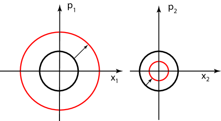
Figure 1: Expanding and contracting phase spaces. Canonical transformations leave the area of each phase space invariant. Non-canonical transformations can change them. Yet the product of these two areas remain invariant.

The contraction of the second phase space has a lower limit in quantum mechanics, namely it cannot become smaller than Planck’s constant. However, there is not such lower limit in classical mechanics. We shall go back to this question in Sec. 5.

In the meantime, let us study what happens when the matrix $G_{3}$ is introduced into the set of matrices given in Eq.(20) and Eq.(21). It commutes with $S_{3},L_{3},K_{1},K_{2},Q_{1}$, and $Q_{2}$. However, its commutators with the rest of the matrices produce four more generators:

$$\left[G_{3},L_{1}\right]=iG_{2},\quad\left[G_{3},L_{2}\right]=-iG_{1},\quad\left[G_{3},K_{3}\right]=iS_{2},\quad\left[G_{3},Q_{3}\right]=-iS_{1},$$ (26)

where

$$G_{1}={i\over 2}\pmatrix{0&I\cr I&0},\qquad G_{2}={1\over 2}\pmatrix{0&-\sigma_{2}\cr\sigma_{2}&0},$$

$$S_{1}={i\over 2}\pmatrix{0&\sigma_{3}\cr-\sigma_{3}&0},\quad S_{2}={i\over 2}\pmatrix{0&-\sigma_{1}\cr\sigma_{1}&0}.$$ (27)

If we take into account the above five generators in addition to the ten generators of $Sp(4)$, there are fifteen generators. These generators satisfy the set of commutation relations given in Eq.(4).

Indeed, the ten $Sp(4)$ generators together with the five new generators form the Lie algebra for the group $SL(4,r)$. There are thus fifteeen four-by-four matrices. They can be written in terms of the fifteen Majorana matrices, as given in Table 1.

Table 2: Three-by-three matrices constituting the two-by-two representation of generators of the $O(3,3)$ group.

	i = 1	i = 2	i = 3
$A_{i}$	$\pmatrix{0&0&0\cr 0&0&-i\cr 0&i&0}$	$\pmatrix{0&0&i\cr 0&0&0\cr-i&0&0}$	$\pmatrix{0&-i&0\cr i&0&0\cr 0&0&0}$
$B_{i}$	$\pmatrix{i&0&0\cr 0&0&0\cr 0&0&0}$	$\pmatrix{0&0&0\cr i&0&0\cr 0&0&0}$	$\pmatrix{0&0&0\cr 0&0&0\cr i&0&0}$
$C_{i}$	$\pmatrix{0&i&0\cr 0&0&0\cr 0&0&0}$	$\pmatrix{0&0&0\cr 0&i&0\cr 0&0&0}$	$\pmatrix{0&0&0\cr 0&0&0\cr 0&i&0}$
$D_{i}$	$\pmatrix{0&0&i\cr 0&0&0\cr 0&0&0}$	$\pmatrix{0&0&0\cr 0&0&i\cr 0&0&0}$	$\pmatrix{0&0&0\cr 0&0&0\cr 0&0&i}$

4.2 Local Isomorphism between O(3,3) and SL(4,r)

It is now possible to write fifteen six-by-six matrices which generate Lorentz transformations on the three space coordinates and three time coordinates [6]. However, those matrices are difficult to handle and do not show existing regularities. In this section, we write those matrices as two-by-two matrices of three-by-three matrices.

For this purpose, we construct four sets of three-by-three matrices given in Table 2. There are two sets of rotation generators

$$L_{i}=\pmatrix{A_{i}&0\cr 0&0},\qquad S_{i}=\pmatrix{0&0\cr 0&A_{i}},$$ (28)

applicable to the space and time coordinates respectively.

There are also three sets of boost generators. In the two-by-two representation of the matrices given in Table 2, they are

$$K_{i}=\pmatrix{0&B_{i}\cr\tilde{B_{i}}&0},\quad Q_{i}=\pmatrix{0&C_{i}\cr\tilde{C_{i}}&0},\quad G_{i}=\pmatrix{0&D_{i}\cr\tilde{D_{i}}&0},$$ (29)

where the three-by-three matrices $A_{i},B_{i},C_{i},$ and $D_{i}$ are given in Table 2, and $\tilde{A_{i}},\tilde{B_{i}},\tilde{C_{i}},\tilde{D_{i}}$ are their transposes respectively.

There is a four-by-four Majorana matrix corresponding to each of hese fifteen six-by-six matrices, as given in Table 1.

There are of course many interesting subgroups. The most interesting case is the $O(3,2)$ subgroup, and there are three of them. Another interesting feature in that there are three time dimensions. Thus, there are also $O(2,3)$ subgroups applicable to two space and three time coordinates. This symmetry between space and time coordinates could be an interesting future investigation.

5 Feynman’s Rest of the Universe

In his book on statistical mechanics [9], Feynman makes the following statement. When we solve a quantum-mechanical problem, what we really do is divide the universe into two parts - the system in which we are interested and the rest of the universe. We then usually act as if the system in which we are interested comprised the entire universe. To motivate the use of density matrices, let us see what happens when we include the part of the universe outside the system.

We can use two coupled harmonic oscillators to illustrate what Feynman says about his rest of the universe. One of the oscillators can be used for the world in which we make physical measurements, while the other belongs to the rest of the universe [8].

Let us start with a single oscillator in its ground state. In quantum mechanics, there are many kinds of excitations of the oscillator, and three of them are familiar to us. First, it can be excited to a state with a definite energy eigenvalue. We obtain the excited-state wave functions by solving the eigenvalue problem for the Schrödinger equation, and this procedure is well known.

Second, the oscillator can go through coherent excitations. The ground-state oscillator can be excited to a coherent or squeezed state. During this process, the minimum uncertainty of the ground state is preserved. The coherent or squeezed state is not in an energy eigenstate. This kind of excited state plays a central role in coherent and squeezed states of light which have recently become a standard item in quantum mechanics.

Third, the oscillator can go through thermal excitations. This is not a quantum excitation, but is a statistical ensemble. We cannot express a thermally excited state by making linear combinations of wave functions. We should treat this as a canonical ensemble. In order to deal with this thermal state, we need a density matrix.

For the thermally excited single-oscillator state, the density matrix takes the form [9, 16, 15].

$$\rho(x,y)=\left(1-e^{-1/T}\right)\sum_{k}e^{-k/T}\phi_{k}(x)\phi_{k}^{*}(x),$$ (30)

where the absolute temperature $T$ is measured in the scale of Boltzmann’s constant, and $\phi_{k}(x)$ is the k-th excited state wave oscillator wave function. The index ranges from $0$ to $\infty$.

We also use Wigner functions to deal with statistical problems in quantum mechanics. The Wigner function for this thermally excited state is [9, 4, 15]

$$W_{T}(x,p)=\frac{1}{\pi}\int e^{-2ipz}\rho(x-z,x+z)dz,$$ (31)

which becomes

$$W_{T}=\left[\frac{\tanh(1/2T)}{\pi}\right]\exp{\left[-\left(x^{2}+p^{2}\right)\tanh(1/2T)\right]}.$$ (32)

This Wigner function becomes

$$W_{0}=\frac{1}{\pi}\exp{\left[-\left(x^{2}+p^{2}\right)\right]},$$ (33)

when $T=0$. As the temperature increases, the radius of this Gaussian form increases from one to [14]

$$\frac{1}{\sqrt{\tanh(1/2T)}}.$$ (34)

The question is whether we can derive this expanding Wigner function from the concept of Feynman’s rest of the universe. In their 1999 paper [8], Han et al. used two coupled harmonic oscillators to illustrate what Feynman said about his rest of the universe. One of their two oscillators is for the world in which we do quantum mechanics and the other is for the rest of the universe. However, these authors did not use canonical transformations. In Subsec. 5.1, we summarize the main point of their paper using the language of canonical transformations developed in the present paper.

Their work was motivated by the papers by Yurke et al. [17] and by Ekert et al. [18], and the Barnett-Phoenix version of information theory [19]. These authors asked the question of what happens when one of the photons is not observed in the two-mode squeezed state.

In Subsec. 5.2, we introduce another form of Feynman’s rest of the universe, based on non-canonical transformations discussed in the present paper. For a two-oscillator system, we can define a single-oscillator Wigner function for each oscillator. Then non-canonical transformations allow one Wigner function to expand while forcing the other to shrink. The shrinking Wigner function has a lower limit in quantum mechanics, while there is none in classical mechanics. Thus, Feynman’s rest of the universe consists of classical mechanics where Planck’s constant has no lower limit.

In Subsec. 5.3, we translate the mathematics of the expanding Wigner function into the physical language of entropy.

5.1 Canonical Approach

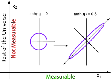
Figure 2: Two-dimensional Gaussian form for two-coupled oscillators. One of the variables is observable while the second variable is not observed. It belongs to Feynman’s rest of the universe.

Let us start with the ground-state wave function for the uncoupled system. Its Hamiltonian is given in Eq.(7), and its wave function is

$$\psi_{0}(x_{1},x_{2})=\frac{1}{\sqrt{\pi}}\exp{\left[-\frac{1}{2}\left(x_{1}^{2}+x_{2}^{2}\right)\right]}.$$ (35)

We can couple these two oscillators by making the following canonical transformations. First, let us rotate the coordinate system by $45^{o}$ to get

$$\frac{1}{\sqrt{2}}\left(x_{1}+x_{2}\right),\qquad\frac{1}{\sqrt{2}}\left(x_{1}-x_{2}\right),$$ (36)

Let us then squeeze the coordinate system:

$$\frac{e^{\eta}}{\sqrt{2}}\left(x_{1}+x_{2}\right),\qquad\frac{e^{-\eta}}{\sqrt{2}}\left(x_{1}-x_{2}\right).$$ (37)

Likewise, we can transform the momentum coordinates to

$$\frac{e^{-\eta}}{\sqrt{2}}\left(p_{1}+p_{2}\right),\qquad\frac{e^{\eta}}{\sqrt{2}}\left(p_{1}-p_{2}\right).$$ (38)

Equations (37) and (38) constitute a very familiar canonical transformation. The resulting wave function for this coupled system becomes

$$\psi_{\eta}(x_{1},x_{2})={1\over\sqrt{\pi}}\exp\left\{-{1\over 4}\left[e^{2\eta}(x_{1}-x_{2})^{2}+e^{-2\eta}(x_{1}+x_{2})^{2}\right]\right\}.$$ (39)

This transformed wave function is illustrated in Fig. 2.

As was discussed in the literature for several different purposes [4, 21, 22, 23], this wave function can be expanded as

$$\psi_{\eta}(x_{1},x_{2})={1\over\cosh\eta}\sum_{k}(\tanh\eta)^{k}\phi_{k}(x_{1})\phi_{k}(x_{2}),$$ (40)

where the wave function $\phi_{k}\phi(x)$ and the range of summation are defined in Eq.(30). From this wave function, we can construct the pure-state density matrix

$$\rho(x_{1},x_{2};x_{1}^{\prime},x_{2}^{\prime})=\psi_{\eta}(x_{1},x_{2})\psi_{\eta}(x_{1}^{\prime},x_{2}^{\prime}),$$ (41)

which satisfies the condition $\rho^{2}=\rho$:

$$\rho(x_{1},x_{2};x_{1}^{\prime},x_{2}^{\prime})=\int\rho(x_{1},x_{2};x_{1}^{\prime\prime},x_{2}^{\prime\prime})\rho(x_{1}^{\prime\prime},x_{2}^{\prime\prime};x_{1}^{\prime},x_{2}^{\prime})dx_{1}^{\prime\prime}dx_{2}^{\prime\prime}.$$ (42)

If we are not able to make observations on the $x_{2}$, we should take the trace of the $\rho$ matrix with respect to the $x_{2}$ variable. Then the resulting density matrix is

$$\rho(x,x^{\prime})=\int\psi_{\eta}(x,x_{2})\left\{\psi_{\eta}(x^{\prime},x_{2})\right\}^{*}dx_{2}.$$ (43)

Here, we have replaced $x_{1}$ and $x^{\prime}_{1}$ by $x$ and $x^{\prime}$ respectively. If we complete the integration over the $x_{2}$ variable,

$$\rho(x,x^{\prime})=\left({1\over\pi\cosh(2\eta)}\right)^{1/2}\exp{\left\{-\left[{(x+x^{\prime})^{2}+(x-x^{\prime})^{2}\cosh^{2}(2\eta)\over 4\cosh(2\eta)}\right]\right\}}.$$ (44)

The diagonal elements of the above density matrix are

$$\rho(x,x)=\left({1\over\pi\cosh(2\eta)}\right)^{1/2}\exp{\left(\frac{-x^{2}}{\cosh(2\eta)}\right)}.$$ (45)

With this expression, we can confirm the property of the density matrix: $Tr(\rho)=1$.

As for the trace of $\rho^{2}$, we can perform the integration

$$Tr\left(\rho^{2}\right)=\int\rho(x,x^{\prime})\rho(x^{\prime},x)dx^{\prime}dx=\frac{1}{\cosh(2\eta)},$$ (46)

which is less than one for nonzero values of $\eta$.

The density matrix can also be calculated from the expansion of the wave function given in Eq.(40). If we perform the integral of Eq.(43), the result is

$$\rho(x,x^{\prime})=\left({1\over\cosh\eta}\right)^{2}\sum_{k}(\tanh\eta)^{2k}\phi_{k}(x)\phi^{*}_{k}(x^{\prime}),$$ (47)

which leads to $Tr(\rho)=1$. It is also straightforward to compute the integral for $Tr(\rho^{2})$. The calculation leads to

$$Tr\left(\rho^{2}\right)=\left({1\over\cosh\eta}\right)^{4}\sum_{k}(\tanh\eta)^{4k}.$$ (48)

The sum of this series becomes to $[1/\cosh(2\eta)]$, as given in Eq.(46).

We can approach this problem using the Wigner function. The Wigner function for the two oscillator system is [4]

$$W_{0}\left(x_{1},p_{1};x_{2},p_{2}\right)=\left(\frac{1}{\pi}\right)^{2}\exp{\left[-\left(x_{1}^{2}+p_{1}^{2}+x_{2}^{2}+p_{2}^{2}\right)\right]}.$$ (49)

If we pretend not to make measurement on the second oscillator coordinate, the $x_{2}$ and $p_{2}$ variables have to be integrated out [8]. The net result becomes the Wigner function for the first oscillator.

The canonical transformation of Eq.(37) and Eq.(38) changes this Wigner function to

$$W(x_{1},x_{2};p_{1},p_{2})=\left(\frac{1}{\pi}\right)^{2}\exp\left\{-{1\over 2}\left[e^{2\eta}(x_{1}-x_{2})^{2}+e^{-2\eta}(x_{1}+x_{2})^{2}\right.\right.$$

$$\mbox{ }\left.\left.+e^{-2\eta}(p_{1}-p_{2})^{2}+e^{2\eta}(p_{1}+p_{2})^{2}\right]\right\}.$$ (50)

If we do not observe the second pair of variables, we have to integrate integrate this function over $x_{2}$ and $p_{2}$:

$$W_{\eta}\left(x_{1},p_{1}\right)=\int W(x_{1},x_{2};p_{1},p_{2})dx_{2}dp_{2},$$ (51)

and the evaluation of this integration leads to [8]

$$W_{\eta}(x,p)=\frac{1}{\pi\cosh\eta}\exp{\left[-\left(\frac{x^{2}+p^{2}}{\cosh(2\eta)}\right)\right]},$$ (52)

where we use $x$ and $p$ for $x_{1}$ and $p_{1}$ respectively.

This Wigner function is of the form given in Eq.(32) for the thermal excitation, if we identify the squeeze parameter $\eta$ as [20]

$$\cosh(2\eta)=\frac{1}{\tanh(1/2T)}.$$ (53)

The failure to make measurement on the second oscillator leads to the radial expansion of the Wigner phase space as in the case of the thermal excitation.

5.2 Non-canonical Approach

As we noted before, among the fifteen Dirac matrices, ten of them can be used for canonical transformations in classical mechanics, and thus in quantum mechanics. They play a special role in quantum optics [2, 3, 4, 5].

The remaining five of them can have their roles if the change in the phase space area is allowed. In quantum mechanics, the area can be increased, but it has a lower limit called Plank’s constant. In classical mechanics, this constraint does not exist. The mathematical formalism given in this paper allows us to study this aspect of the system of coupled oscillators.

Let us choose the following three matrices from those in Eq.(20) and Eq.(21).

$$S_{3}={1\over 2}\pmatrix{\sigma_{2}&0\cr 0&\sigma_{2}},\quad K_{2}={i\over 2}\pmatrix{\sigma_{3}&0\cr 0&\sigma_{3}},\quad Q_{2}={i\over 2}\pmatrix{\sigma_{1}&0\cr 0&\sigma_{1}}.$$ (54)

They satisfy the closed set of commutation relations:

$$\left[S_{3},K_{2}\right]=iQ_{2},\quad\left[S_{3},Q_{2}\right]=-iQ_{3},\quad\left[K_{2},Q_{2}\right]=-iS_{3}.$$ (55)

This is the Lie algebra for the $Sp(2)$ group, This is the symmetry group applicable to the single-oscillator phase space [4], with one rotation and two squeezes. These matrices generate the same transformation for the first and second oscillators.

We can choose three other sets with similar properties. They are

$$S_{3}={1\over 2}\pmatrix{\sigma_{2}&0\cr 0&\sigma_{2}},\quad Q_{1}={i\over 2}\pmatrix{\sigma_{3}&0\cr 0&-\sigma_{3}},\quad K_{1}={i\over 2}\pmatrix{\sigma_{1}&0\cr 0&-\sigma_{1}},$$

$$L_{3}={1\over 2}\pmatrix{-\sigma_{2}&0\cr 0&\sigma_{2}},\quad K_{2}={i\over 2}\pmatrix{\sigma_{3}&0\cr 0&\sigma_{3}},\quad K_{1}={i\over 2}\pmatrix{-\sigma_{1}&0\cr 0&\sigma_{1}},$$

and

$$L_{3}={1\over 2}\pmatrix{-\sigma_{2}&0\cr 0&\sigma_{2}},\quad-Q_{2}={i\over 2}\pmatrix{-\sigma_{3}&0\cr 0&\sigma_{3}},\quad Q_{2}={i\over 2}\pmatrix{\sigma_{1}&0\cr 0&\sigma_{1}}.$$ (56)

These matrices also satisfy the commutation relations given in Eq.(55). In this case, the squeeze transformations take opposite directions in the second phase space.

Since all these transformations are canonical, they leave the area of each phase space invariant. However, let us look at the non-canonical generator $G_{3}$ of Eq.(25). It generates the transformation matrix of the form

$$\pmatrix{e^{\eta}&0\cr 0&e^{-\eta}}.$$ (57)

If $\eta$ is positive, this matrix expands the first phase space while contracting the second. This contraction of the second phase space is allowed in classical mechanics, but it has a lower limit in quantum mechanics.

The expansion of the first phase space is exactly like the thermal expansion resulting from our failure to observe the second oscillator which belongs to the rest of the universe. If we expand the system of Dirac’s ten oscillator matrices to the world of his fifteen Majorana matrices, we can expand and contract the first and second phase spaces without mixing them up. We can thus construct a model where the observed world and the rest of the universe remain separated. In the observable world, quantum mechanics remains valid with thermal excitations. In the rest of the universe, since the area of the phase space can become small without lower limit, only classical mechanics is valid.

During the expansion/contraction process, the product of the areas of the two phase space remains constant. This may or may not be an extended interpretation of the the uncertainty principle, but we choose not to speculate further on this issue.

Let us turn our attention to the fact that the groups $SL(4,r)$ and $Sp(4)$ are locally isomorphic to $O(3,3)$ and $O(3,2)$ respectively. This means that we can do quantum mechanics in one of the $O(3,2)$ subgroups of $O(3,3)$, as Dirac noted in his 1963 paper [1]. The remaining generators belong to Feynman’s rest of the universe.

5.3 Entropy and the Expanding Wigner Phase Space

We have seen how Feynman’s rest of the universe increases the radius of the Wigner function. It is important to note that the entropy of the system also increases.

Let us go back to the density matrix. The standard way to measure this ignorance is to calculate the entropy defined as [16, 24, 25, 26, 27]

$$S=-Tr\left(\rho\ln(\rho)\right),$$ (58)

where $S$ is measured in units of Boltzmann’s constant. If we use the density matrix given in Eq.(47), the entropy becomes

$$S=\cosh^{2}\eta\ln\left(\cosh^{2}\eta\right)-\sinh^{2}\eta\ln\left(\sinh^{2}\eta\right).$$ (59)

In order to express this equation in terms of the temperature variable $T$, we write Eq.(53) as

$$\cosh(2\eta)=\frac{1+e^{-1/T}}{1-e^{-1/T}},$$ (60)

which leads to

$$\cosh^{2}\eta=\frac{1}{1-e^{-1/T}},\qquad\sinh^{2}\eta=\frac{e^{-1/T}}{1-e^{-1/T}}.$$ (61)

Then the entropy of Eq.(59) takes the form [8]

$$S=\left(\frac{1}{T}\right)\left\{\frac{1}{\exp{(1/T)}-1}\right\}-\ln\left(1-e^{-1/T}\right).$$ (62)

This familiar expression is for the entropy of an oscillator state in thermal equilibrium. Thus, for this oscillator system, we can relate our ignorance of the Feynamn’s rest of the universe, measured by of the coupling parameter $\eta$, to the temperature.

6 Concluding Remarks

In this paper, we started with the fifteen four-by-four matrices for the Majorana representation of the Dirac matrices, and the ten generators of the $Sp(4)$ group corresponding to Dirac’s oscillator matrices. Their explicit forms are given in the literature [6, 7], and their roles in modern physics are well known [3, 4, 11]. We re-organized them into tables.

The difference between these two representations consists of five matrices. The physics of this difference is discussed in terms of Feynman’s rest of the universe [9]. According to Feynman, this universe consists of the world in which we do quantum mechanics, and the rest of the universe. In the rest of the universe, our physical laws may or may not be respected. In the case of coupled oscillators, without the lower limit on Planck’s constant, we can do classical mechanics but not quantum mechanics in the rest of the universe.

In 1971, Feynman et al. [30] published a paper on the oscillator model of hadrons, where the proton consists of three quarks linked up by oscillator springs. In order to treat this problem, they use a three-particle symmetry group formulated by Dirac in his book on quantum mechanics [31, 32]. An interesting problem could be to see what happens to the two quarks when one of them is not observed. Another interesetinq question could be to see what happens to one of the quarks when two of them are not observed.

Finally, we note here that group theory is a very powerful tool in approaching problems in modern physics. Different groups can share the same set of commutation relations for their generators. Recently, the group $SL(2,c)$, through its correspondence with the $SO(3,1)$ has been shown to be the underlying language for classical and modern optics [4, 28]. In this paper, we exploited the correspondence between $SL(4,r)$ and $O(3,3)$, as well as the correspondence between $Sp(4)$ and $O(3,2)$ which was first noted by Paul A. M. Dirac[1].

There could be more applications of group isomorphisms in the future. A comprehensive list of those correspondences is given in Gilmore’s book on Lie groups [29].

References

• [1] Dirac, P. A. M.; A Remarkable Representation of the 3 + 2 de Sitter Group. J. Math. Phys. 1963, 4, 901-909.
• [2] Yuen, H. P.; Two-photon coherent states of the radiation field. Phys. Rev. A 1976, 13, 2226-2243.
• [3] Yurke, B. S.; L. McCall, B. L.; Klauder, J. R.; SU(2) and SU(1,1) interferometers. Phys. Rev. A 1986, 33, 4033-4054.
• [4] Kim, Y. S.; Noz, M. E.; Phase Space Picture of Quantum Mechanics. World Scientific Publishing Company: Singapore 1991.
• [5] Han, D.; Kim, Y.S.; Noz, M. E.; Yeh, L.; Symmetries of Two-mode Squeezed States. J. Math. Phys. 1993, 34, 5493-5508.
• [6] Han,D.; Kim, Y. S.; Noz, M. E.; O(3,3)-like Symmetries of Coupled Harmonic Oscillators. J. Math. Phys. 1995, 36, 3940-3954.
• [7] D. Lee, J.; The Dirac gamma matrices as “relics” of a hidden symmetry?: As fundamental representation of the algebra Sp(4,r). J. Math. Phys. 1995, 36, 524-530.
• [8] Han, D.; Kim, Y. S.; Noz, M. E.; Illustrative Example of Feynman’s Rest of the Universe. Am. J. Phys. 1999, 67, 61-66.
• [9] Feynman, R. P.; Statistical Mechanics. Benjamin/Cummings: Reading, Massachusetts 1972.
• [10] Majorana, E.; Relativistic Particles with Arbitrary Instrisic Angular Momenum. Nuovo Cimento 1932, 9, 335-341.
• [11] Itzykson, C.; Zuber, J. B.; Quantum Field Theory. MaGraw-Hill, New York 1980.
• [12] Goldstein, H.; Classical Mechanics, 2nd ed. Addison-Wesley, Reading, Massachusetts 1980.
• [13] Abraham, R.; Marsden, J. E.; Foundations of Mechanics, 2nd ed. Benjamin/Cummings, Reading, Massachusetts 1978.
• [14] Kim, Y. S.; Li, M.; Squeezed States and Thermally Excited States in the Wigner Phase-Space Picture of Quantum Mechanics. Phys. Lett. A 1989, 139, 445-448.
• [15] Davies, R. W.; Davies, K. T. R.; On the Wigner distribution function for an oscillator. Ann. Phys. 1975, 89, 261-273.
• [16] Landau, L. D.; Lifshitz, E. M.; Statistical Physics. Pergamon Press, London 1958.
• [17] Yurke, B; Potasek, M.; Obtainment of Thermal Noise from a Pure State. Phys. Rev. A 1987, 36, 3464-3466.
• [18] Ekert, A. K.; Knight, P. L.; Correlations and squeezing of two-mode oscillations. Am. J. Phys. 1989, 57, 692-697.
• [19] Barnett, S. M.; Phoenix,S.J.D.; Information Theory, Squeezing and Quantum Correlations. Phys. Rev. A 1991, 44, 535-545.
• [20] Han, D.; Kim, Y. S.; Noz, M. E.; Lorentz-Squeezed Hadrons and Hadronic Temperature. Phys. Lett. A 1990, 144, 111-115.
• [21] Kim, Y. S.; Noz, M.E.; Oh, S. H.; A Simple Method for Illustrating the Difference between the Homogeneous and Inhomogeneous Lorentz Groups, Am. J. Phys. 1979 47, 892-897.
• [22] Kim, Y. S.; Noz, M. E.; Theory and Applications of the Poincaré Group. Reidel, Dordrecht 1986.
• [23] Giedke, G.; Wolf, M.M.; Krueger, O; Werner, R.F.; Cirac, J.J. Entanglement of formation for symmetric Gaussian states. Phys. Rev. Lett. 2003, 91, 107901-107904.
• [24] von Neumann, J; Mathematical Foundation of Quantum Mechanics Princeton University 1955.
• [25] Fano, U; Description of States in Quantum Mechanics by Density Matrix and Operator Techniques. Rev. Mod. Phys. 1957, 29, 74-93.
• [26] Blum, K.; Density Matrix Theory and Applications. Plenum, New York 1981.
• [27] Kim, Y. S.; Wigner, E. P.; Entropy and Lorentz Transformations. Phys. Lett. A 1990, 147, 343-347.
• [28] S. Başkal, S.; Kim, Y. S.; Lorentz Group in Ray and Polarization Optics. in Mathematical Optics: Classical, Quantum and Imaging Methods, edited by Vasudevan Lakshminarayanan, Taylor and Francis, New York 2012.
• [29] Gilmore, R.; Lie Groups, Lie Algebras, and Some of Their Applications. Wiley, New York 1974.
• [30] Feynman, R. P.; Kislinger, M.; Ravndal F; Current Matrix Elements from a Relativistic Quark Model. Phys. Rev. D1971 3, 2706-2732.
• [31] Dirac, P. A. M.; Principles of Quantum Mechanics, 4th Ed. Oxford University, London1958.
• [32] Hussar, P. E.; Kim, Y. S.; Noz, M. E.; Three-Particle Symmetry Classifications according to the Method of Dirac. Am. J. Phys. 1980 48, 1038-1042.