1

A Self-Organized Neural Comparator

Guillermo A. Ludueña¹ and Claudius Gros^1
1Institute for Theoretical Physics, Goethe University - Frankfurt am Main, Germany.

Keywords: Neural Networks, Self-organization, Complex Systems

Abstract

Learning algorithms need generally the possibility to compare several streams of information. Neural learning architectures hence need a unit, a comparator, able to compare several inputs encoding either internal or external information, like for instance predictions and sensory readings. Without the possibility of comparing the values of prediction to actual sensory inputs, reward evaluation and supervised learning would not be possible.
Comparators are usually not implemented explicitly, necessary comparisons are commonly performed by directly comparing one-to-one the respective activities. This implies that the characteristics of the two input streams (like size and encoding) must be provided at the time of designing the system.
It is however plausible that biological comparators emerge from self-organizing, genetically encoded principles, which allow the system to adapt to the changes in the input and in the organism. We propose an unsupervised neural circuitry, where the function of input comparison emerges via self-organization only from the interaction of the system with the respective inputs, without external influence or supervision.
The proposed neural comparator adapts, unsupervised, according to the correlations present in the input streams. The system consists of a multilayer feed-forward neural network which follows a local output minimization (anti-Hebbian) rule for adaptation of the synaptic weights.
The local output minimization allows the circuit to autonomously acquire the capability of comparing the neural activities received from different neural populations, which may differ in the size of the population and in the neural encoding used. The comparator is able to compare objects never encountered before in the sensory input streams and to evaluate a measure of their similarity, even when differently encoded.

1 Introduction

In order to develop a complex targeted behavior, an autonomous agent must be able to relate and compare information received from the environment with internally generated information (see Billing, 2010). For example it is often necessary to decide whether the visual image currently being perceived is similar to an image encoded in some form in memory.

For artificial agents, such basic comparison capabilities are typically either hard-coded or initially taught, both processes involving the inclusion of predefined knowledge (for instance Bovet and Pfeifer, 2005a, b). However, living organisms must acquire this capability autonomously, only via interaction with the acquired data, possibly without any explicit feedback from the environment (O’Reilly and Munakata, 2000). We can therefore hypothesize the presence of a neural circuitry in living organisms, capable of comparing the information received by different populations of neurons. It cannot therefore in general be assumed that these populations have a similar configuration, hold the information in the same encoding or even manage the same type of information.

A system encompassing said characteristics must be based on some form of unsupervised learning, it must self-organize in order to autonomously acquire its basic functionality. The task of an unsupervised learning system is to elucidate the structure in the input data, without using external feedback. Thus all the information should be inferred from the correlations found in the input and in its own response to the input data stream.

Unsupervised learning can be achieved using neural networks, and has been implemented previously for a range of applications (see for instance Sanger, 1989; Atiya, 1990; Likhovidov, 1997; Furao et al., 2007; Tong et al., 2008). Higher accuracy is generally expected from supervised algorithms. However, Japkowicz et al. (1995); Japkowicz (2001) have shown that for the problem of binary classification, unsupervised learning in a neural network can perform better than standard supervised approaches in certain domains.

Neural and non-biologically inspired algorithms are often expressed in mathematical terms based on vectors and their respective elementary operations like vector subtraction, conjunction and disjunction. Implementations in terms of artificial neural networks hence typically involve the application of these operations to the output of groups of neurons. These basic operations are however not directly available in biological neural circuitry, which is based exclusively on local operations. Connections between groups of neurons evolve during the growth of the biological agent and may induce the formation of topological maps (see Kohonen, 1990) but generically do not result in one-to-one neural operations. For instance these one-to-one neural interactions would involve an additional global summation of the result for the case of a scalar product.

It is unclear whether operations like vector operations are directly used by biological systems, their implementation should be in any case robust to the changes in the development of the system and to its adaptation to different types of input. In effect, the basic building blocks of most known learning algorithms are the mathematical functions computers are based on. These are, however, not necessarily present, convenient or viable in a biological system. It is our aim to elucidate how a basic mathematical function can emerge naturally in a biological system. We present, for this purpose, a model of how the basic function of comparison can emerge in an unsupervised neural network, based on local rules for adaption and learning. Our adaptive “comparator” neural circuit is capable of self-organized adaption, with the correlations present in the data input stream as the only basis for inference.

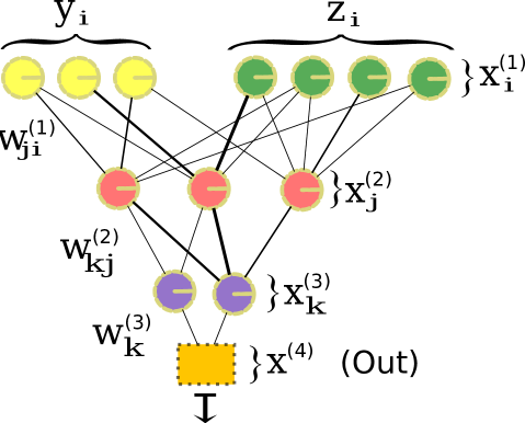
Figure 1: Architecture of the proposed neural comparator, with intermediate layers $\mathbf{x}^{(2)}$ and $\mathbf{x}^{(3)}$ and output $\mathbf{x}^{(4)}$. The comparator autonomously learns to compare the inputs $\mathbf{y}$ and $\mathbf{z}$. The output is close to zero when the two inputs are identical or correlated and close to unity when they are different or uncorrelated.

The circuit autonomously acquires the capability of comparing the information received from different neural populations, which may differ in size and in the encoding used. The comparator proposed is based on a multilayer feed-forward neural network, where the input layer receives two signals $\mathbf{y}$ and $\mathbf{z}$, see fig. 1. These two input streams can be either unrelated, selected randomly or, with a probability, encode the same information. The task of the neural comparator is then to determine, for any pair of input signals $\mathbf{y}$ and $\mathbf{z}$, whether they are semantically related or not. Any given pair ($\mathbf{y}$,$\mathbf{z}$) of semantically related inputs is presented to the system, in general, only one single time. The system has hence to master the task of discriminating generically between related and unrelated pairs of inputs, and not the task to extract statistically repeatedly occurring patterns.

The strength of the synapses connecting neurons are readjusted using anti-Hebbian rules. Due to the readjustment of the synaptic weights, the network minimizes its output without the help of external supervision. As a consequence, the network is able to autonomously learn to discriminate whether the two inputs encode the same information or not, independently of whether the particular input configuration has been encountered before or not. The system will respond with a large output activity whenever the input pair ($\mathbf{y}$,$\mathbf{z}$) is semantically unrelated and with inactivity for related pairs.

1.1 Motivation and expected use case

We are motivated by a system where the information stored in two different neuronal populations are to be compared. In particular, we are interested in systems as the one presented by Bovet and Pfeifer (2005a), where two streams of information (for instance, visual input and the desired state of the visual input, or the signal from the whiskers of a robot compared to the time-delayed state of these sensors) encoded in two separate neuronal populations are to be compared, in this particular case in order to get a distance vector between the two. In a fixed artificial system, one could obtain this difference by simply subtracting the input from each of the streams, provided that the two neuronal populations are equal and encode the information in the same way. This subtraction can also be implemented in such a system in a neuromorphic way simply by implementing a distance function in a neural network. However, we are interested in the case where both neuron populations have evolved mostly independently, such that they might be structurally different and might encode the information in a different way, which is expected in a biological system. Under these conditions, the neuronal circuit comparing both streams should be able to invert the encoding of both inputs in order to compare them, a task which could not be solved using a fixed distance function. In addition, we expect that such a system would be deployed in an environment where it is more probable to have different, semantically unrelated, inputs than otherwise. The comparator should hence be able to solve the demanding task of autonomously extracting semantically related pairs of inputs out of a majority of unrelated and random input patterns.

2 Architecture of the neural comparator

The neural comparator proposed consists of a feed-forward network of three layers, plus an extra layer filtering the maximum output from the third layer, compare fig. 1. We will refer to the layers as $k=1,2,3,4$, where $k=1$ corresponds to the input layer and $k=4$ to the output layer. The output of the individual neurons is denoted by $x_{i}^{(k)}$, where the supraindex refers to the layer and the subindex to the index of the neuron in the layer, for instance $x_{2}^{(1)}$ being the output of the second neuron in the input layer.

The individual layers are connected via synaptic weights $w_{ji}^{(k)}$. In this notation, the index $i$ corresponds to the index of the presynaptic neuron in layer $k$, and $j$ corresponds to the index of the postsynaptic neuron in layer $k+1$. Thus $w_{3,4}^{(1)}$ is the synaptic weight connecting the fourth input neuron with the third neuron in the second layer.

The layers are generally not fully interconnected. The probability of a connection between a neuron in layer $k$ and a neuron in layer $k+1$ is $p_{conn}^{(k)}$. The values used for the interconnection probabilities $p_{conn}^{(k)}$ are given in table 1.

In the implementation proposed and discussed here, the output layer is special in that it consists only in selecting the maximum of all activities from the third layer. There are simple neural architectures based on local operations that could fulfill this purpose. However, for simplicity, the task of selecting the maximum activity of the third layer is done here directly by a single unit.

2.1 Input protocol

The input vectors $\mathbf{x}^{(1)}$ consist of two parts

$$\mathbf{x}^{(1)}\ =\ \big{(}\mathbf{y},\mathbf{z}\big{)}~{},$$ (1)

where $\mathbf{y}$ and $\mathbf{z}$ are the two distinct input streams to be compared. We used the following protocol for selecting pairs of $(\mathbf{y},\mathbf{z})$:

• $\mathbf{y}$ is selected randomly at each time step, with the elements $y_{i}\in[0,1]$ drawn from a uniform distribution.

• $\mathbf{z}$ is selected via

  $$\mathbf{z}\ =\ \left\{\begin{array}[]{rl}\mathrm{random}&\mathrm{with\ probability}\ 1-p_{eq}\\ \mathbf{f}(\mathbf{y})&\mathrm{with\ probability}\ p_{eq}\end{array}\right.$$ (2)

If the inputs $\mathbf{z}$ and $\mathbf{y}$ carry the same information, they are related via $\mathbf{z}=\mathbf{f}(\mathbf{y})$, where $\mathbf{f}$ is generically an injective transformation. This relation reduces to $\mathbf{z}=\mathbf{y}$ for the case when the encodings in the two neural populations $y$ and $z$ are the identity.

We consider two kinds of encoding, direct encoding with $\mathbf{f}$ being the identity, and encoding through a linear transformation, which we refer as “linear encoding”,

$$\mathbf{z}=\mathbf{y}\qquad\mathrm{or}\qquad\mathbf{z}=\hat{A}\mathbf{y}\;,$$ (3)

where $\hat{A}$ is a random matrix. The encoding is maintained throughout individual simulations of the comparator. For the case of linear encoding, the matrix $\hat{A}$ is selected initially and not modified during a single run.

The procedure we used to generate the matrix $\hat{A}$ consists of choosing each element of the matrix as a random number taken from a continuous flat distribution of values between -1 and 1. The matrix is then normalized such that the elements of vector $\mathbf{z}$ belong to $z_{i}=[-1,1]$.

2.2 Synaptic weights readjustment: anti-Hebbian rule

Each neuron integrates its inputs, via

$$x_{j}^{(k+1)}=g\left(\sum_{i}{w^{(k)}_{ji}x_{i}^{(k)}}\right),\qquad g(x)=\tanh(\alpha x)~{},$$ (4)

with $g(x)$ being the transfer function, $\alpha$ the gain and $w^{(k)}_{ji}$ the afferent synaptic weights. After the information is passed forward, the synaptic weights are corrected using an anti-Hebbian rule,

$$\Delta w_{ji}^{(k)}(t) \equiv w_{ji}^{(k)}(t+1)-w_{ji}^{(k)}(t)$$ (5)

$$= -\eta x_{i}^{(k)}(t)x_{j}^{(k+1)}(t)\;.$$

Neurons under an anti-Hebbian learning rule will modify their synaptic weights in order to minimize their output. Note, that anti-Hebbian adaption rules generically result from information maximization principles (Bell and Sejnowski, 1995). Information maximization favors spread-out output activities for statistically independent inputs (Marković and Gros, 2010), allowing such to filter-out correlated input pairs $(\mathbf{y},\mathbf{z})$, which tend to induce a low level of output activities.

The incoming synaptic weights to neuron $i$ of the $(k+1)$th layer are additionally normalized, after an update of the synaptic weights,

$$w_{ji}^{(k)}(t+1)\ \to\ \frac{w_{ji}^{(k)}(t+1)}{\sqrt{\sum_{j}\big{|}w_{ji}^{(k)}(t+1)\big{|}^{2}}}\;.$$ (6)

The algorithm proposed here is based on the idea that correlated inputs will lead to a small output, as a consequence of the anti-Hebbian adaption rule. Uncorrelated pairs of input $(\mathbf{y},\mathbf{z})$ will on the other side generate, in general, a substantial output, as they correspond to random inputs for which the synaptic weights are not adapted to minimize the output. It is worthwhile to remark that using a Hebbian adaption rule and classifying the minimum values as uncorrelated would not achieve the same accuracy as with the proposed anti-Hebbian rule with output values between -1 and 1. The reason is that we seek a comparator capable of comparing arbitrary pairs $(\mathbf{y},\mathbf{z})$ of input, and not specific examples.

When using an anti-Hebbian rule, zero output is an optimum for any correlated input. In the case of input with equal encoding, this is reached when the synaptic weights cancel exactly ($w_{left}=-w_{right}$) in the first layer, compare fig. 1. In contrast, if a Hebbian rule would be used, the optimum value for correlated input corresponds to the synaptic weights of correlated input being as large as possible. The consequence is that all synaptic weights tend to increase constantly, eventually leading to all output achieving maximum values.

There remains, for anti-Hebbian adaption rules, a statistically finite probability for uncorrelated inputs to have a low output by mere chance, viz the terms $w_{ji}^{(k)}x^{(k)}_{i}$ originating from $\mathbf{y}$ and $\mathbf{z}$ may cancel out. In such cases the comparator would be misclassifying the input. The occurrence of misclassification is reduced substantially by having multiple neurons in the third layer.

By selecting an inter-layer connection probability $p_{conn}^{(2)}$ well below unity, the individual neurons in the third layer will have access to different components of the information encoded in the second layer. This setup is effectively equivalent to generating different and independent parallel paths for the information transfer, adding robustness to the learning process, since only strong correlations between the input pairs $(\mathbf{y},\mathbf{z})$, shared by the majority of paths, are then acquired by all neurons.

In addition to diminishing the possibility of random misclassification due to the multiple paths, the use of anti-Hebbian learning in the third layer minimizes the incidence of the individual parallel paths which consistently result in $x_{i}^{(2)}$ outputs that are far larger than the rest (failing paths, since they are unable to learn some correlations). Thus adding this layer results in an significant increase in accuracy with respect to an individual 2-layer comparator. The accuracy is further improved by adding a filtering layer for input classification.

2.3 Input classification

Each third-layer neuron encodes the estimated degree of correlation within the input pairs, $(\mathbf{y},\mathbf{z})$. The fourth layer selects the most active third-layer neuron,

$$x^{(4)}\ =\ \max_{j}|x_{j}^{(3)}|\;.$$ (7)

By selecting the maximum of all outputs in the third layer, the circuit looks for a “consensus” among the neurons in the third layer. A given input pair ($\mathbf{y}$,$\mathbf{z}$) needs to be considered as correlated by all third-layer neurons in order to be classified as correlated by the fourth layer. This, together with the randomness of the inter-layer connections, increases the robustness of the classification process.

There are several options for evaluating the effectiveness of the neural comparator. We will later discuss, in sect. 4, an analysis in terms of fuzzy logic, and consider now a measure of the accuracy of the system in terms of binary classification. The inputs $\mathbf{y}$ and $\mathbf{z}$ are classified according to the strength of the value of $x^{(4)}$. For binary classification we use a simple threshold criterion. The inputs $\mathbf{y}$ and $\mathbf{z}$ are considered to be uncorrelated if

$$x^{(4)}\ >\ \theta\;,$$

and otherwise correlated. In this work, the value for the threshold $\theta$ is determined by minimizing the probability of misclassification, in order to test the possible accuracy of the system. The same effect of this minimization could be achieved by keeping $\theta$ fixed and optimizing the slope $\alpha$ of the transfer function (4), since $\theta$ depends on the slope $\alpha$. These parameters, the slope $\alpha$ or the discrimination threshold $\theta$, may in principle be optimized autonomously using information theoretical objective functions Triesch (2005); Marković and Gros (2010). For simplicity we here perform the optimization directly. We will show in sec. 3.4, that the optimal values for $\alpha$ and $\theta$ depend essentially only on the size $N$ of the input. Minor adjustments of the parameters might anyway be desirable to maintain an optimal accuracy. In any case, these readjustments can be done in a biological system via intrinsic plasticity (see Stemmler and Koch, 1999; Mozzachiodi and Byrne, 2010; Marković and Gros, 2011).

Although we did not implement the $max$ function present in (7) in a neuromorphic form, a small neuronal circuit implementing (7) could for instance be realized as a winner-takes-all network (Coultrip et al., 1992; Kaski and Kohonen, 1994; Carpenter and Grossberg, 1987). Alternatively, a filtering rule different from the $max$ function could be used for the last layer, for instance the addition or averaging of all the inputs. We present as supporting information some results showing the behavior of the output when using averaging and sum as alternative filtering rules for the output layer. Our best results were however found by implementing the last layer as a $max$ function. In this work we will discuss the behavior of the system using the $max$ function as the last layer.

We would like to remark that defining a threshold $\theta$ is one way of using this system for binary classification, which we use for reporting the possible accuracy of the system. However, it is not a defining part of the model. We expect the system to be more useful for obtaining a continuous variable measuring the grade of correlation of the inputs. As we discuss in sec. 4, this property can be used to apply fuzzy logic in a biological system.

3 Performance in terms of binary classification

3.1 Performance measures

In order to access the performance, in terms of binary classification, of the neural comparator, we need to track the numbers of correct and incorrect classifications. We use the following three measures for classification errors:

• false positives: The fraction of cases for which $x^{(4)}<\theta$ (input is classified as correlated) occurs for uncorrelated pairs of input vectors $\mathbf{y}$ and $\mathbf{z}$:

  $$FP\ =\ \frac{\mathrm{\#\,erroneously\,assigned\,as\,positive}}{\mathrm{\#assigned\,as\,positive}}\;.$$ (8)

• false negatives: The fraction of cases with output activity $x^{(4)}\geq\theta$ (input classified as uncorrelated) occurring for correlated pairs of input vectors, $\mathbf{z}=\mathbf{f}(\mathbf{y})$:

  $$FN\ =\ \frac{\mathrm{\#\,erroneously\,assigned\,as\,negative}}{\mathrm{\#assigned\,as\,negative}}\;.$$ (9)

• overall error: The total fraction of errors $E$ is the fraction of overall wrong classifications:

  $$E\ =\ \frac{\mathrm{\#\,erroneously\,assigned}}{\mathrm{\#all\,assignments}}\;.$$ (10)

All three performance measures, $E$, $FP$ and $FN$, need to be kept low. This is achieved for a classification threshold $\theta$ which minimizes $(FP+FN)$. This condition keeps all three error measures, $FP$, $FN$ and $E$ close to their minimum, while giving $FN$ and $FP$ equal importance at the same time.

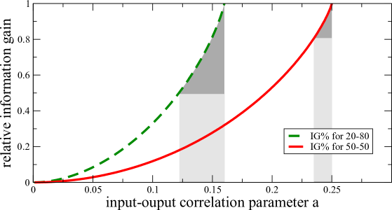
Figure 2: The relative mutual information MI% (3.1), as a function of the amount of correlation $a$ between the input and the output, defined by eq. 13. The comparator achieves an MI% of about 50% and 80% respectively for fractions of $p_{eq}=0.2$ (dashed line) and $p_{eq}=0.8$ (solid line) of correlated input pairs, corresponding to $0.12/0.16=0.75$ and $0.23/0.25=0.92$ of all input-output correlations $a$. Hence only 25% and 8%, respectively (darker shaded areas), of all correlations are not recovered by the comparator.

3.1 Mutual Information

Since the percentage of erroneous classifications, despite it being an intuitive measure, is dependent on the relative number of correlated and uncorrelated inputs presented to the system, we also evaluate the mutual information (MI) (see for instance Gros, 2008) as a measure of the information that has been gained by the classification made by the comparator:

$$\mathrm{MI}(X,Y) = H[X]-H[X|Y]$$

$$= -\sum_{x\in X}p(x)\log{(p(x))}+\sum_{y\in Y}p(y)\sum_{x\in X}p(x|y)\log{(p(x|y))}\;,$$

where $X$ in this case represents whether the inputs are equal or not, and $Y$ is whether the comparator classified the input as correlated or not, therefore, both $X$ and $Y$ are vectors of size two ($true/false$ corresponding to semantically related/uncorrelated). Here $\rho(x|y)$ is the conditional probability that the input had been $x=frue/false$ given that output of the comparator is $y=true/false$ and $H(X)$ the marginal information entropy.

We will refer specifically to the mutual information (3.1) between the binary input and output of the neural comparator, also known in this context as information gain. The mutual information (3.1) can also be written as $\sum_{x,y}p(x,y)\log(p(x,y)/(p(x)p(y)))$, where $p(x,y)=p(y|y)p(y)$ is the joint probability. It is symmetric in its arguments $X$ and $Y$ and positive definite. It vanishes for uncorrelated processes $X$ and $Y$, viz when $\rho(x|y)=\rho(x)$, viz for a random output of the comparator. Finally, the mutual information is maximal when the two processes are 100% correlated, that is, when the off-diagonal probability vanish, $\rho(x|y)=0$ for $x\neq y$. In this case the two marginal distributions $\rho(x)=\sum_{y}p(x,y)$ and $\rho(y)=\sum_{x}p(x,y)$ coincide and $MI(X,Y)$ is identical to coinciding marginal entropies, $H(X)=H(Y)$.

We will present the mutual information as the percentage of the maximally achievable mutual information,

$$\mathrm{MI\%}(X,Y) = \frac{H[X]-H[X|Y]}{H[X]}$$

$$= 1-\frac{\sum_{y\in Y}p(y)\sum_{x\in X}p(x|y)\log{(p(x|y))}}{\sum_{x\in X}p(x)\log{(p(x))}}\;,$$

which has hence a value between 0 and 1, and is therefore more intuitive to read as a percentage of the maximum theoretically possible. The maximum mutual information achievable by the system depends solely on the probabilities of correlation/decorrelation, i.e. $p_{eq}$.

The statistical correlations between the input $X$ and the output $Y$ can be parametrized using a correlation parameter $a$, via

$$p(x,y)\ =\ p(x)\,p(y)\ +C_{a}(x,y)~{},$$ (13)

where $C_{a}(x,y)$ are the element values of the matrix:

$$C_{a}=\left(\begin{array}[]{cc}a&-a\\ -a&a\end{array}\right)\qquad\quad a\in\big{[}0,p_{eq}(1-p_{eq})\big{]}~{}.$$ (14)

Here $p_{eq}$ is the probability of having correlated pairs of inputs, viz $p(x=true)=p_{eq}$ and $p(x=false)=(1-p_{eq})$. Using this parametrization allows us to evaluate the relative mutual information (3.1) generically for a correlated joint probability $p(x,y)$, as illustrated in fig. 2. The parametrization (13) hence provides an absolute yardstick for the performance of the neural comparator.

3.2 Simulation results

We performed a series of simulations using the network parameters listed in table 1, and for two encoding rules (2), direct and linear encoding. The lengths $N$ of the input vectors $\mathbf{y}$ and $\mathbf{z}$ are taken to be equal, if not stated otherwise.

Param.	$t_{max}$	$N^{(1)}$	$N^{(2)}$	$N^{(3)}$	$\alpha$ ($N<400$)
Value	$10^{7}$	2$N$	$N$	$\lfloor\frac{N+1}{2}\rfloor$	2.7
Param.	$p_{conn}^{(1)}$	$p_{conn}^{(2)}$	$\eta$	$p_{eq}$	$\alpha$ ($N\geq 400$)
Value	0.8	0.3	0.003	0.2	1.0

Table 1: Parameters used in the simulations. $N$: Input vector size, $N^{(k)}$: size of layer $k$, $t_{max}$: number of steps of simulation, $p_{eq}$: probability of equal inputs, $p_{conn}^{(k)}$: probability of connection from the $k$th layer to the $(k+1)$th layer, $\alpha$: sigmoid slope, $\eta$: learning rate.

3.1 Low Probability of Equals

Since our initial motivation for the design of this system is the comparison of two input streams that are presumably most of the time different, we have studied the behavior of the system when there is a lower probability of an event where both streams are equal than otherwise. We used $p_{eq}=0.2$ in (2), viz in 20% of the cases the relation $\mathbf{z}=\mathbf{f}(\mathbf{y})$ holds and in the remaining 80% the two inputs $\mathbf{y}$ and $\mathbf{z}$ are completely uncorrelated (randomly drawn). Each calculation consists of $t_{max}=10^{7}$ steps, from which the last 10% of the simulation is used for the evaluation of the performance. During said last 10% of the simulation the system keeps learning, i.e. there is no separation between training and production stages. The purpose of taking only the last portion is to ignore the initial phase of the learning process, since at that stage the output does not provide a good representation of the system’s accuracy.

In table 2, we present the mean values for the different measures of error, eqs. (8)–(10), observed for 100 independent simulations of the system. For each individual simulation, the interlayer connections are randomly drawn with probabilities $p_{conn}^{(k)}$, the parameters are as shown in table 1. The errors for each run are calculated using a threshold $\theta$ that minimizes the sum of errors $\langle FP\rangle+\langle FN\rangle$. Each input in the first layer has a uniform distribution of values between -1 and 1. The accuracy of the comparator is generally above 90%, in terms of binary classification errors. There is, importantly, no appreciable difference in the accuracy when using direct encoding or linear encoding with random matrices.

Note, that a relative mutual information of MI%$\approx$50% is substantial (Guo et al., 2005). A relative mutual information of 50% means that the correlation between the input and the output of the neural comparator encompasses 75% of the maximally achievable correlations, as illustrated in fig. 2.

	direct				linear
$N$	$\langle E\rangle$	$\langle FP\rangle$	$\langle FN\rangle$	MI%	$\langle E\rangle$	$\langle FP\rangle$	$\langle FN\rangle$	MI%
5	10.2%	5.8%	10.5%	13.2%	14.8%	8.3%	14.8%	23.8%
15	6.0%	1.2%	6.8%	44.4%	5.2%	2.8%	5.9%	41.7%
30	5.3%	1.0%	6.0%	49.5%	4.8%	1.3%	5.4%	50.8%
60	6.6%	0.6%	7.4%	45.3%	4.3%	1.0%	5.0%	54.7%
100	6.5%	0.5%	7.5%	45.5%	5.3%	0.6%	6.1%	51.5%
200	7.8%	0.9%	8.8%	37.3%	6.2%	0.9%	7.2%	44.2%
400	7.1%	0.8%	7.5%	43.5%	7.2%	0.7%	8.1%	41.5%
600	-	-	-	-	6.7%	0.5%	7.0%	50.8%

Table 2: Errors obtained from averaging 100 runs of the comparator, using direct and linear encoding after $10^{7}$ steps, for different input sizes $N$. The connection probabilities used are $p_{conn}^{(1)}=0.3$, $p_{conn}^{(2)}=0.8$. For $N>5$ the standard deviations amounts to 0.1-0.8% (decreasing with $N$) for the errors E, FP and FN, and 1% for MI%. For the $N=5$ case, the standard deviation of the errors is 5-14% (again, decreasing with $N$) while for MI% it amounts to 15%.

We found that the performance of the comparator depends substantially on the degree of similarity of the two input signals $\mathbf{y}$ and $\mathbf{z}$ for the case when the two inputs are uncorrelated. For a quantitative evaluation of this dependency we define the Euclidean distance

$$d=\left|\left|\mathbf{y}-\mathbf{f}^{-1}(\mathbf{z})\right|\right|\;,$$ (15)

where $||\cdot||$ denotes the Euclidean norm of a vector. For small input sizes $N$, a substantial fraction of the input vectors are relatively similar with small Euclidean distance $d$, resulting in a small output $x^{(4)}$. This can prevent the comparator from learning the classification effectively, thus the best accuracy is obtained for input vectors of size greater than $N=10$, compare table 2.

The above phenomenon can be investigated systematically by considering two distinct distributions for the Euclidean distance $d$. Within our input protocol (2) the pairs $\mathbf{y}$ and $\mathbf{z}$ are statistically independent with probability $(1-p_{eq})$. We have considered two ways of generating statistically unrelated input pairs,

Unconstrained: The components $$y_{i} z_{i} [-1,1]$$ and are selected randomly from the interval . (16)

and

Constrained: The components $$y_{i} z_{i} d [0,1]$$ and are selected randomly such that the distance has a flat (uniform) distribution in . (17)

For the case of the ‘unconstrained’ input protocol the distribution of distances $d$ is sharply peaked for large input size $N$, compare fig. 3. The impact of the distribution of Euclidean distances between the random input vectors $\mathbf{y}$ and $\mathbf{z}$ is presented in fig. 3, where we show the result of three separated simulations:

• Using the unconstrained input protocol (16) for both training and for testing. The corresponding performance errors are $FP=1.0\%$, $FN=10.7\%$ and $E=9.7\%$, for a threshold $\theta=0.34$.

• Using the unconstrained input protocol (16) for training and the constrained (17) protocol for testing. The performance errors are $FP=13.7\%$, $FN=14.6\%$ and $E=14.2\%$, for a threshold $\theta=0.28$.

• Using the constrained input protocol (17) for both training and testing. The corresponding errors are $FP=79.9\%$, $FN=0.0\%$ and $E=79.9\%$, for a threshold $\theta=0.02$.

The accuracy of the comparator is very good for a). In this case values close to $d\sim 0$ are almost inexistent for random input pairs $\mathbf{y}$ and $\mathbf{z}$, random and related input pairs are clustered in distinct parts of the phase space.

The performance of the comparator drops, on the other side, with increasing number of similar random input pairs. For the case c) the distribution of distances $d$ is uniform and the comparator has essentially no comparison capabilities. Since the 20% of the input is correlated, the minimal error $E$ in this case is obtained if the system assumes all input to be uncorrelated (i.e. setting an extremely small threshold). That situation results in 80% $FP$ and 20% $FN$. Notice that in this case the mutual information of the system is null. Lastly, in the mixed case b) the comparator is trained with a unconstrained distribution for the distances $d$ and tested using a constrained distribution. In this case the comparator still acquires a reasonable accuracy of $E=14\%$.

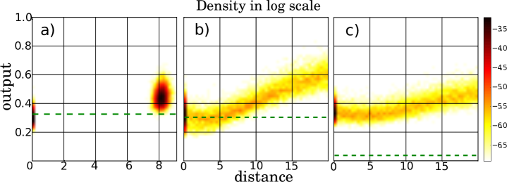
Figure 3: The probability of an output $x^{(4)}$ (7) to occur as a function of Euclidean distance $d$ (15) of the input pairs $\mathbf{y}$ and $\mathbf{z}$ (see fig. 1), as a density plot (color coded), using $N=400$, $\alpha=1$ and direct encoding. The last 10% of simulations with $10^{7}$ input pairs have been taken for the performance testing. a) Unconstrained input protocol (16) both for training and for testing b) Unconstrained input protocol (16) for training and constrained (17) for testing. c) Constrained input protocol (17) for both training and testing.

3.2 Equilibrated Input, $p_{eq}=0.5$

In this subsection we expand the results for equilibrated input data sets, viz $p_{eq}=0.5$ in (2). The procedure remains as described in the previous section. Again, each calculation consists of $t_{max}=10^{7}$ steps, from which the last 10% of the simulation is used for performance evaluation. This result is consistent with the intuitive notion, that it is substantially harder to learn when $\mathbf{y}$ and $\mathbf{z}$ are related, when most of the input stream is just random noise and semantically correlated input pairs occur only seldom. For applications one may hence consider a training phase with a high frequency $p_{eq}$ of semantically correlated input pairs.

$N$	$\langle E\rangle$	$\langle FP\rangle$	$\langle FN\rangle$	MI%
5	9$\pm$6 %	8$\pm$7 %	10$\pm$5 %	58$\pm$14 %
15	3.9$\pm$0.4 %	0.4$\pm$0.1 %	6.9$\pm$0.6 %	78$\pm$1 %
30	3.4$\pm$0.2 %	0.3$\pm$0.1 %	6.3$\pm$0.3 %	81$\pm$1 %
60	3.3$\pm$0.1 %	0.2$\pm$0.1 %	6.1$\pm$0.2 %	81$\pm$1 %
100	3.4$\pm$0.1 %	0.2$\pm$0.1 %	6.2$\pm$0.1 %	82$\pm$1 %
200	4.7$\pm$0.1 %	0.5$\pm$0.3 %	8.2$\pm$0.5 %	75$\pm$1 %
400	6.2$\pm$0.1 %	0.4$\pm$0.1 %	10.9$\pm$0.1 %	70$\pm$1 %
600	7.5$\pm$0.1 %	1.1$\pm$0.1 %	12.4$\pm$0.1 %	66$\pm$1 %

Table 3: Errors obtained from averaging 100 runs of the comparator, using linear encoding, with $p_{eq}=0.5$, for different input sizes $N$. The connection probabilities used are $p_{conn}^{(1)}=0.3$, $p_{conn}^{(2)}=0.8$.

As seen in table 3, the use of a balanced input set does not change the general behavior but results in a substantial increase in performance. The accuracy of the system in terms of percentage of correct classifications (above 95% accuracy except on very small input size) and relative mutual information MI% ($\sim 80\%$ of the maximum information gain) is very high. A relative mutual information of MI%$\approx$80% means that the system recovers over 92% of the maximally achievable correlations between the input and the output, as shown in fig. 2.

3.3 Effect of noisy encoding

In the previous sections we have provided results showing that the proposed comparator can achieve a good accuracy despite the fact that a large part of the input is noise. In addition, the comparator is also robust against a level of noise in the encoding of the inputs. Random noise in the encoding would correspond to the neural populations having rapid random reconfigurations or random changes in the individual neurons’ behavior above a certain level.

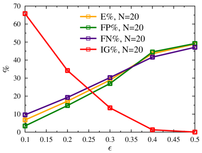
Figure 4: Errors $E$, $FP$, $FN$, and percentage of information gain MI% for different levels of noise $\epsilon$ in the encoding. $\epsilon=0.5$ corresponds to a magnitude equal to the average activity of an input.

As shown in fig. 4, the system has an accuracy decay if the encoding is affected by random noise of the same magnitude as the average input activity (0.5). For this calculation, we define the random noise in the encoding as adding a random number between 0 and $\epsilon$ to each element of one of the compared inputs, i.e. $y_{i}\to y_{i}+r_{i}$, where $r_{i}\in[0,\epsilon]$. The values $r_{i}$ are changed in every step of the calculation.

The addition of random noise in the encoding is effectively seen by the system as a slightly different input. Since the system is designed to classify inputs either into different or equal, a large level of noise drives the system into classifying the input as different. However, if the input is only slightly changed, the correlation is still found by the comparator and the output remains under the threshold for classification.

3.4 Impact of the frequency of correlated input and input size

In fig. 5, the dependency of the optimal threshold $\theta$ and the errors $E,FP,FN,$ MI% with the probability $p_{eq}$ is shown. At a constant input size, the threshold shows only a weak dependence with the probability $p_{eq}$. The threshold changes at its maximum for the probability of any case in the order of 10% or less. The threshold varies less than 0.1 from $p_{eq}=0.1$ to $p_{eq}=0.9$. This indicates that the system would still be effective if the probabilities of the events change significantly, even without readjusting the parameters $\alpha$ or $\theta$, or with a small readjustment if the change is extreme.

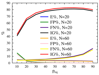
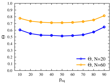
Figure 5: On the left, the errors $E$, $FP$, $FN$, and relative mutual information MI% for different frequencies of correlated input $p_{eq}$ (percentages). The results are presented for input sizes $N=$ 20 and 60. On the right, the optimal values of the threshold $\theta$ for different frequencies of correlated input $p_{eq}$. The results are again presented for input sizes $N=$ 20 and 60.

In fig. 6, the dependence of the optimal threshold $\theta$ with the input size $N$ is presented. The threshold has a marked logarithmic dependency with respect to the system size. In effect, the threshold $\theta$, the gain $\alpha$ and the system size $N$ are all strongly coupled, such that given an input size the rest of the parameters are essentially fixed.

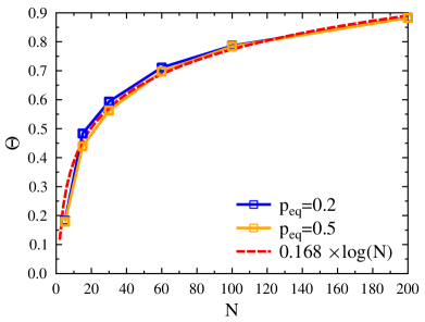
Figure 6: Optimal threshold $\theta$ vs input size $N$, for $\alpha=2.7$. The behavior is markedly logarithmic.

3.5 Comparison of inputs with different sizes

	$N=20$				$N=60$
$\Delta$	$\langle E\rangle$	$\langle FP\rangle$	$\langle FN\rangle$	MI%	$\langle E\rangle$	$\langle FP\rangle$	$\langle FN\rangle$	MI%
0	3.4$\pm$0.3	0.3$\pm$0.1	6.3$\pm$0.4	80$\pm$1	3.3$\pm$0.1	0.2$\pm$0.1	6.1$\pm$0.2	81$\pm$1
5	3.1$\pm$0.3	0.3$\pm$0.1	5.7$\pm$0.5	82$\pm$1	3.4$\pm$0.3	0.3$\pm$0.1	6.3$\pm$0.2	80$\pm$1
10	2.7$\pm$0.2	0.3$\pm$0.1	4.9$\pm$0.4	84$\pm$1	2.9$\pm$0.1	0.2$\pm$0.1	5.4$\pm$0.2	83$\pm$1
20	2.2$\pm$0.2	0.3$\pm$0.1	4.0$\pm$0.4	86$\pm$1	2.6$\pm$0.1	0.2$\pm$0.1	4.8$\pm$0.1	85$\pm$1
40	1.6$\pm$0.1	0.3$\pm$0.1	2.9$\pm$0.3	89$\pm$1	2.2$\pm$0.1	0.2$\pm$0.1	4.0$\pm$0.1	87$\pm$1

Table 4: Average errors $\langle E\rangle$, $\langle FP\rangle$, $\langle FN\rangle$ and relative mutual information MI% obtained from 100 runs of the comparator for comparing one input of size $N=20$ ($N=60$, right) and another of size $N+\Delta$, using $p_{eq}=50$.

The comparator successfully compares input of different sizes. In table 4 we show the average accuracy over 100 runs of a comparator where one of the vectors to be compared has a size $N$ and the other has a larger size $N+\Delta$. The number of extra inputs $\Delta$ is maintained constant during the whole simulation. In each step, the values of the two vectors are assigned as described previously as “linear encoding” in sec. 2.1. The linear encoding is done in this case with a matrix $\hat{A}$ that has dimensions $(N+\Delta)\times N$, thus the information gets encoded in a vector of higher dimension.

The accuracy of the comparator does not decrease, but, rather surprisingly, it slightly increases. There is no loss in accuracy because the uncorrelated inputs are not minimized to a value close to zero due to the anti-Hebbian adjustment of the synaptic weights, as happens only with the correlated input. We attribute the small increase in accuracy to the increase of neurons involved in the system.

3.6 Influence of connection density

A key ingredient in this model is the suppression of a fraction of inter-layer connections with probability $1-p_{conn}$, which is necessary to give higher-layer neurons the possibility to encode varying features of correlated input pairs. For a systematic study we ran simulations using a range of distinct probabilities of interconnecting the layers.

In figure 7, we show the unconstrained performance measures for $N=5$ when changing (left) the connection $p_{conn}^{(1)}$ from the input layer to the first layer (compare fig. 1, with constant $p_{conn}^{(2)}=0.75$) and (right) when varying the connection $p_{conn}^{(2)}$ from the second to the third layer. In the later case we kept $p_{conn}^{(1)}=0.3$ fixed.

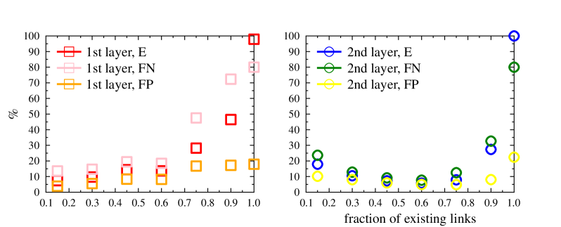
Figure 7: Effect of the probability of connection in the overall errors. On the left, the errors of the comparator with varying probability $p_{conn}^{(1)}$ of connection efferent from the first layer, with $p_{conn}^{(2)}=0.75$. On the right, the probability $p_{conn}^{(2)}$ of efferent connection from the second layer is varied, keeping $p_{conn}^{(1)}=0.3$ constant.

The data presented in fig. 7 show that the neural comparator loses functionality when the network becomes fully interconnected. The optimal interconnection density varies from layer to layer and is best for 10% efferent first-layer connections and 60% links efferent from the second layer.

3.7 Images Comparison

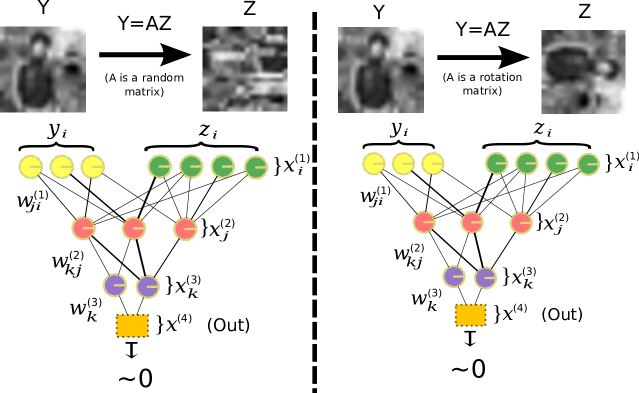
Figure 8: Scheme of two possible encryptions made by the comparator with probability $p_{eq}$. In both cases, after being exposed to many images the comparator would ideally result in an output $x^{4}\sim 0$. Notice the matrix $A$ in each side of the figure is constant during the whole simulation.

We tested the comparator efficiency in comparing a set of black and white pictures of small size (20$\times$20 pixels, i.e. $N=400$) using linear encoding via a random matrix as in previous sections, see fig. 8. The set of pictures is very small (200 pictures) in comparison to the input data used to train the comparator ($t=10^{7}$ inputs). The results can be seen in table 5. The limited input set has the negative effect that the comparator is not able to learn comparison only from this set. This suggests that in order for the comparator to develop its functionality, it must sample a sizable part of the possible input patterns.

	$\langle E\rangle$	$\langle FP\rangle$	$\langle FN\rangle$	MI%
Only Images $p_{eq}=0.2$	20.6$\pm$0.3	51.9$\pm$0.6	14.4$\pm$0.2	8$\pm$1
Trained w/Random input $p_{eq}=0.2$	14.5$\pm$0.2	39.3$\pm$0.3	6.2$\pm$0.1	32$\pm$1
Trained w/Random input $p_{eq}=0.5$	10.8$\pm$0.1	10.7$\pm$0.2	10.9$\pm$0.1	51$\pm$1

Table 5: Average errors $\langle E\rangle$, $\langle FP\rangle$, $\langle FN\rangle$ and relative mutual information MI% obtained from 100 runs of the comparator for comparing black and white pictures of size 20$\times$20 pixels.

As explained previously, the correlated inputs are minimized by the anti-Hebbian rule, while the uncorrelated input cannot be minimized to the same level, since those cases result in the terms $x_{i}^{(k)}x_{j}^{(k+1)}$ in eq. (5) being essentially random. This assumption is however not fulfilled if the values of these terms are not well distributed (unless their values are by chance always small), which is the case if the sampling is not large enough.

As a second test, we initially trained the comparator using random data (still using $p_{eq}=0.5$) in order to start with a functional distribution of the synaptic weights, and then switched to the picture set for the last 10% of the calculation, with the comparator still learning during this stage. In this case, the comparator achieved its function (see table 5). However, the accuracy did not fully reach that of the system when comparing randomly generated data.

We expect the accuracy of the random comparator to be at the level of the generated by random input if the input stream explores a sizable part of the possible input. For instance, ideally the image input would be a video of the visual input in a mobile agent while exploring the environment, such that a large amount of patterns are processed by the comparator. This is however out of the scope for this work, while follow up work is expected.

4 Interpretation within the scope of fuzzy logic

The dependency of the output of the comparator seen in fig. 3b,c and fig. 9 can be interpreted in terms of fuzzy logic (Keller et al., 1992), offering alternative application scenarios for the neural comparator.

The error measures evaluated in table 2, like the incidence of false positives ($FP$), are based on boolean logic, the classification is either correct or incorrect, i.e. binary. For real-world applications the input pairs $(\mathbf{y},\mathbf{z})$ may be similar but not equal and the dependency of the output as a function of input similarity is an important relation characterizing the functionality of neural comparators.

The comparator essentially provides a continuous variable classifying how much the input case corresponds to the case of equal input, i.e. a truth degree. Thus, the comparator can be interpreted as a fuzzy logic gate for the operator “equals” ($=$), since it provides a truth degree for the outcome of the discrete version of the same operator.

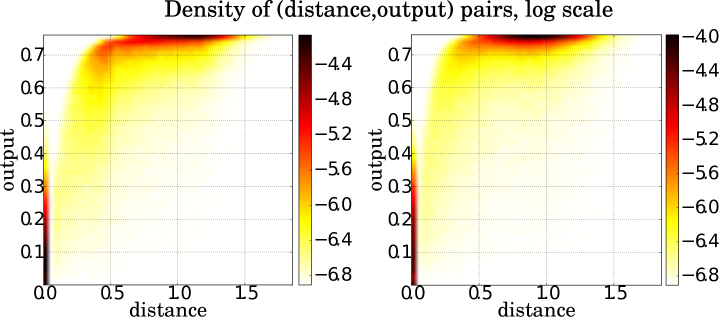
Figure 9: Density of output-distance pairs from two individual runs of the comparator, comparing inputs of dimension $N=5$ under the direct encoding (left) and linear encoding (right), using $\alpha=2.7$.

In fig. 9 we present, on a logarithmic scale, the density of results for the observed output $x^{(4)}$, as a function of the distance $d$ between the respective inputs, for one single run of the comparator. $80\%$ of the input vectors were randomly drawn and later readjusted in order to fill the range of distances $d=0.1$ to $1.5$ uniformly, according to the constrained protocol (17). In addition, $20\%$ of the input have a distance of $d=0$ with $\mathbf{z}=\mathbf{y}$, resulting in the high density of simulations at $d=0$.

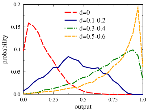
Figure 10: Output distribution for different Euclidean distances $d$ (15) between the inputs, as a function of output, corresponding to a vertical slice of the $N=5$ direct encoding data presented in fig. 9.

The uncertainty of the classification of inputs presented in fig. 9 is reflected in a probability distribution for the comparator output, shown in fig. 10 for the case of direct encoding. The output distribution is narrower for cases where the distance $d$ corresponds to clearly correlated or uncorrelated inputs.

The distributions presented in fig. 9 can be interpreted as fuzzy probability distributions for any given distance $d$ (vertical slices), as shown in fig. 10. The probability for the input pairs $\mathbf{y}$ and $\mathbf{z}$ to be classified as different decreases with decreasing distance $d$ between them. This shows that inputs with smaller distances have in general increasingly weaker outputs. Thus, assuming that the Euclidean distance $d$ is a good estimator of how similar the input is, the output of the comparator provides an arguably reliable continuous variable estimating a similarity degree for the inputs, i.e. the truth degree of the operator “equals” applied to the inputs.

5 Discussion

The results presented here demonstrate that the proposed neural comparator has the capability of discerning similar input vectors from dissimilar ones, even under noisy conditions. Using 80% noise, with four out of five inputs being randomly drawn, the unsupervised comparator architecture achieves a boolean discrimination accuracy of above $\sim$90%. The comparator circuit can also achieve the same accuracy when the inputs to be compared are encoded differently. If the encodings of both inputs are related by a linear relation, the accuracy of the comparison does not worsen with respect to the direct encoding case.

A key factor for the accuracy of the method is the inclusion of a slightly different path for the layer-to-layer information, provided by random suppressions of interlayer connections. However, the suppression has the potential side effect of rendering some of the correlations difficult to be learned. For this reason a compromise needs to be found between the number of connections that must be kept in order to maintain the network functional and the number of connections that needs to be removed to generate sufficiently different outputs in the third layer.

We find it remarkable that from a very simple model of interacting neurons under the rule of minimization of its output, the fairly complex task of identifying the similarity between unrelated inputs can emerge through self-organization without the need of any predefined or externally given information. Complexity arising from simple interactions is a characteristic of natural systems, and we believe the capacity of many living beings to perform comparison operations could potentially be based on some of the aspects included in our model.

Conclusion

We have presented a neuronal circuit based on a feed-forward artificial neural network, which is able to discriminate whether two inputs are equal or different with high accuracy even under noisy input conditions.

Our model is an example of how algorithmic functionalities can emerge from the interaction of individual neurons under strictly local rules, in our case the minimization of the output, without hard-wired encoding of the algorithm, without external supervision and without any a priori information about the objects to be compared. Since our model is capable of comparing information in different encodings, it would be a suitable model of how seemingly unrelated information coming from different areas of a brain can be integrated and compared.

We view the architecture proposed here as a first step towards an in-depth study of the important question: which are possible neural circuits for the unsupervised comparison of unknown objects. Our results show, that anti-Hebbian adaption rules, which are optimal for synaptic information transmission (Bell and Sejnowski, 1995), allow to compare two novel objects, viz objects never encountered before during training, with respect to their similarity. The model is capable not only to provide binary answers – whether the two objects in the sensory stream are (are not) identical – but also to give a quantitative estimate of the degree of similarity, which may be interpreted in the context of fuzzy logic. We believe this quantitative estimate of similarity to be a central aspect of any neural comparator, as it may be used as a learning or reenforcement signal.

References

- Atiya (1990) A.F. Atiya (1990). An unsupervised learning technique for artificial neural networks. Neural Networks, 3, 707–711.
- Bell and Sejnowski (1995) A.J. Bell, and T. Sejnowski. An information-maximization approach to blind separation and blind deconvolution. Neural Computing, 7, 1129–1159.
- Billing (2010) E.A. Billing (2010). Cognitive perspectives on robot behavior. In Proceedings of the 2nd International Conference on Agents and Artificial Intelligence: Special Session on Computing Languages with Multi-Agent Systems and Bio-Inspired Devices, pages 373–382.
- Bovet and Pfeifer (2005a) S. Bovet and R. Pfeifer (2005). Emergence of coherent behaviors from homogeneous sensorimotor coupling. In Proceedings of the 12th International Conference on Advanced Robotics (ICAR)a.
- Bovet and Pfeifer (2005b) S. Bovet and R. Pfeifer (2005). Emergence of delayed reward learning from sensorimotor coordination. In Proceedings of the IEEE/RSJ International Conference on Intelligent Robots and Systems (IROS)b.
- Carpenter and Grossberg (1987) G.A. Carpenter and S. Grossberg (1987). A massively parallel architecture for a self-organizing neural pattern recognition machine. Computer Vision, Graphics, and Image Processing, 37, 54–115.
- Coultrip et al. (1992) R. Coultrip, R. Granger, and G. Lynch (1992). A cortical model of winner-take-all competition via lateral inhibition. Neural Networks, 5, 47–54.
- Furao et al. (2007) S. Furao, T. Ogura, and O. Hasegawa (2007). An enhanced self-organizing incremental neural network for online unsupervised learning. Neural Networks, 20, 893 – 903.
- Gros (2008) C. Gros (2008). Complex and Adaptive Dynamical Systems, a Primer. Springer, New York.
- Guo et al. (2005) D. Guo, S. Shamai, and S. Verdú, Mutual information and minimum mean-square error in Gaussian channels. IEEE Transactions on Information Theory, 51, 1261–1282.
- Japkowicz (2001) N. Japkowicz (2001). Supervised versus unsupervised binary-learning by feedforward neural networks. Machine Learning, 42, 97–122.
- Japkowicz et al. (1995) N. Japkowicz, C. Myers, and M. Gluck (1995). A novelty detection approach to classification. In Proceedings of the Fourteenth Joint Conference on Artificial Intelligence, pages 518–523.
- Kaski and Kohonen (1994) S. Kaski and T. Kohonen (1994). Winner-take-all networks for physiological models of competitive learning. Neural Networks, 7, 973–984.
- Keller et al. (1992) J.M. Keller, R.R. Yager, and Tahani (1992). Neural network implementation of fuzzy logic. Fuzzy Sets and Systems, 45, 1–12.
- Kohonen (1990) T. Kohonen (1990). The self-organizing map. Proceedings of the IEEE, 78, 1464–1480.
- Likhovidov (1997) V. Likhovidov (1997). Variational approach to unsupervised learning algorithms of neural networks. Neural Networks, 10, 273–289.
- Marković and Gros (2010) D. Marković and C. Gros (2011). Self-organized chaos through polyhomeostatic optimization. Physical Review Letters, 105, 068702.
- Marković and Gros (2011) D. Marković and C. Gros (2011). Intrinsic adaptation in autonomous recurrent neural networks. Neural Computation, 24, 523–540.
- Mozzachiodi and Byrne (2010) R. Mozzachiodi and J.H. Byrne (2010). More than synaptic plasticity: role of nonsynaptic plasticity in learning and memory. Trends in Neurosciences, 33, 17–26.
- O’Reilly and Munakata (2000) R.C. O’Reilly and Y. Munakata (2000). Computational Explorations in Cognitive Neuroscience. The MIT press. Cambridge, Massachusetts. London, England..
- Sanger (1989) T.D. Sanger (1989). Optimal unsupervised learning in a single-layer linear feedforward neural network. Neural Networks, 2, 459–473.
- Stemmler and Koch (1999) M. Stemmler and C. Koch (1999). How voltage-dependent conductances can adapt to maximize the information encoded by neuronal firing rate. Nature Neuroscience, 2, 521–527.
- Triesch (2005) J. Triesch (2005). A gradient rule for the plasticity of a neuron’s intrinsic excitability. Artificial Neural Networks: Biological Inspirations - ICANN 2005, 65–70.
- Tong et al. (2008) H. Tong, T. Liu, and Q. Tong (2008). Unsupervised learning neural network with convex constraint: Structure and algorithm. Neurocomputing, 71, 620–625.