Calculation of binding energies and masses of quarkonia in analytic QCD models111 In comparison with v1: improved presentation; (F)APT calculation performed in the scheme; comparison with the results of other methods in the literature included (cf. Table IV); part of the text moved into the new Appendix A; the basic conclusions unchanged; extended acknowledgments; Refs. [12,38-39,41,44,80-83,89-99,110-11] are new.
Abstract
We extract quark masses () from the evaluation of the masses of quarkonia and , performed in two analytic QCD models, and in perturbative QCD in two renormalization schemes. In analytic QCD the running coupling has no unphysical singularities in the low-momentum regime. We apply the analytic model of Shirkov et al. [Analytic Perturbation Theory (APT)], extended by Bakulev et al. [Fractional Analytic Perturbation Theory (FAPT)], and the two-delta analytic model (2anQCD). The latter, in contrast to (F)APT, at higher energies basically coincides with the perturbative QCD (in the same scheme). We use the renormalon-free mass as input. The separation of the soft and ultrasoft parts of the binding energy is performed by the requirement of the cancellation of the leading infrared renormalon. The analysis in the 2anQCD model indicates that the low-momentum ultrasoft regime is important for the extraction of the masses , especially . The 2anQCD model gives us clues on how to estimate the influence of the ultrasoft sector on in general. These effects lead to relatively large values GeV in the 2anQCD model, which, however, are compatible with recent lattice calculations. In perturbative QCD in scheme these effects are even stronger and give larger uncertainties in . The (F)APT model gives small ultrasoft effects and the extracted values of agree with those in most of the literature ( GeV). The extracted values of in all four models are about - GeV and agree well with those in the literature.
pacs:
12.38.Cy, 12.38.Aw,12.40.VvI Introduction
Most of the calculations of the masses of heavy quarkonia are based on perturbative expansions. These expansions come from the knowledge of the static quark-antiquark potential which has been calculated up to () in Refs. Peter:1996ig ; Schroder:1998vy . At () level, ultrasoft gluons contribute Brambilla:1999qa ; Kniehl:1999ud to and the calculation of these terms has been completed in Refs. Smirnov:2009fh ; Anzai:2009tm . The expansion coefficients for the mass of the (heavy) quarkonium vector () or scalar () ground state (i.e., with: and ) are given, for example, in Ref. Penin:2002zv , for the terms including . The latter term is known because the potential is known at level. For a review of the topic, see, e.g. Ref. Pineda:2011dg .
Most of the radiative contributions to the quarkonium mass expansion are from the so called soft sector of gluon momenta, .222 The momentum transfer of the gluon is spacelike, i.e., , because the scattering of the quark and antiquark in the quarkonium is of the -channel type. In the cases of and , these are around GeV and GeV, respectively. At GeV scales, the perturbative QCD (pQCD) coupling is marginally reliable; at GeV it is unreliable. This is so because the pQCD coupling suffers from unphysical (Landau) singularities at low spacelike (), i.e., at where ; for it is dangerously close to these singularities, and thus unreliable.
The aforementioned Landau singularities are not physical because they do not possess the analytic properties of the spacelike observables (such as the Adler function), the latter properties being dictated by the general properties of quantum field theories BS ; Oehme including causality. Namely, must be an analytic function in the entire complex plane, with the exception of the timelike semiaxis , where GeV is a particle production threshold. Specifically, the evaluation of spacelike quantities in pQCD, as a (truncated) power series of the perturbative running coupling (couplant) (with ), does not respect these important analytic properties of . These problems, within the context of QCD, were first addressed in the seminal works of Shirkov, Solovtsov, Milton et al. ShS ; MS ; MSS ; Solovtsov:1997at ; Sh1 ; Sh2 . There, the perturbative running coupling was made an analytic (in the aforementioned sense) function of , , in the following way: in the dispersion relation the discontinuity function was kept unchanged on the entire negative axis in the complex -plane (i.e., for ), and was set equal to zero on the nonphysical cut . For this reason, this analytic QCD (anQCD) model can be referred to as the minimal analytic (MA) model. Here we will refer to this model by its usual name used in the literature: Analytic Perturbation Theory (APT).
Various other analytic QCD (anQCD) models for can be constructed, and have been presented in the literature, among them Refs. Nesterenko ; Nesterenko2 ; Alekseev:2005he ; Srivastava:2001ts ; Webber:1998um ; CV1 ; CV2 ; Bdecays ; Shirkov:2012ux . These models fulfill certain additional constraints at low and/or at high . For further literature on various analytic QCD models, we refer to the review articles in Refs. Prosperi:2006hx ; Shirkov:2006gv ; Cvetic:2008bn ; Bakulev . Some newer constructions of anQCD models of include those based on specific classes of functions with nonperturbative contributions Belyakova:2010iw or without such contributions CKV1 ; CKV2 , and those based on modifications of the discontinuity function [ ] at low (positive) where is parametrized in a specific manner (with delta functions), cf. Refs. 1danQCD ; 2danQCD .
The model of Ref. 2danQCD , an extension of the model of Ref. 1danQCD , will be called the two-delta analytic QCD model (2anQCD), because its discontinuity function is parametrized in the unknown low- regime by two delta functions. It has a specific attractive feature that in the high-scale regime () it practically coincides with the corresponding (in the scheme) pQCD coupling: . This makes it possible for the model to be applied with the Operator Product Expansion (OPE) anOPE including terms of dimension without the need to modify the ITEP school (Institute of Theoretical and Experimental Physics) interpretation of the OPE Shifman:1978bx ; DMW . The latter basically states that the terms in OPE of higher dimension () originate from the infrared regime only.
Once we have an anQCD model, i.e., a model for the analytic analog of the pQCD coupling (or, equivalently, for the discontinuity function ), the analytic analogs of the higher powers have to be constructed from . In the case of APT (), for integer , the couplings were constructed in Refs. MS ; MSS ; Solovtsov:1997at . However, perturbation expansions of some observables, and effects of evolution of distribution amplitudes at a chosen loop-level, are represented sometimes by noninteger powers or logarithmic terms ( noninteger, integer). Among them are the pion electromagnetic form factor and hadronic decay width of Higgs . The problems of the analytization of such quantities, within the spirit of APT, were considered in Ref. KS , where the dispersion relations were extended from the coupling parameter to the general QCD amplitudes. The APT approach to evaluation of the (factorizable part) of the form factor was performed in Ref. Baketal , where the nonperturbative distribution amplitude was evaluated by performing numerical evolution with an analytic coupling parameter. The authors Bakulev, Mikhailov and Stefanis (BMS) then systematically extended APT in Ref. BMS1 to the evaluation of noninteger power analogs and of the mentioned terms and . This extension was performed for the spacelike quantities, with explicit expressions at the one-loop level, and extension to the higher-loop level via expansions of the one-loop expressions. This was then applied to an evaluation of the factorizable part of in Ref. BKS . In Ref. BMS2 the BMS authors extended this construction to the timelike quantities and applied it to the evaluation of the Higgs decay width in APT. In Ref. BMS3 this construction was applied to the evaluation of the ratio , and a detailed analysis of the evaluation of . In the review work of Bakulev, Ref. Bakulev , several variants of this construction are reviewed, among them the numerical dispersive approach at the two-loop and higher-loop level (Secs. III B, C, D of Ref. Bakulev ); a mathematical package for such numerical calculation is given in Ref. BK . The construction of BMS is referred to in the literature as the Fractional Analytic Perturbation Theory (FAPT).
In the general case of analytic , the quantities were constructed in Refs. CV1 ; CV2 for integer , as linear combinations of logarithmic derivatives (),333The relations between such functions ’s and ’s, allowing a recurrent construction of , for integer within the context of the APT model, were given also in Refs. Shirkov:2006nc ; Shirkov:2006gv . and were extended to noninteger in Ref. GCAK .
In this work, we apply two anQCD models of , namely APT of Refs. ShS ; MS ; MSS ; Solovtsov:1997at ; Sh1 ; Sh2 , and the 2anQCD model of Refs. 2danQCD ; anOPE , to evaluations of the perturbation series of the binding energy of heavy quarkonia ( and ) and of the quark pole mass . In this way, we will evaluate the masses of these quarkonia as functions of the () quark mass . In the APT model of analytic QCD (i.e., the model for , Ref. ShS ), we will need to evaluate not just the integer power analogs , but also the analogs of the logarithmic terms whose evaluation uses the approach of FAPT BMS1 ; BMS2 , reviewed in Bakulev . Therefore, we will refer to this method as APT when it involves only integer power analogs, and as (F)APT when it involves both aforementioned types of terms.
As input parameter we use the renormalon-free quark mass () of the corresponding quark (also called the quark mass), and the anQCD coupling of the model. Since the quarkonia masses are well measured, we can extract the values of . We also perform the same analysis in pQCD in the corresponding renormalization schemes.
In Sec. II we briefly describe the (F)APT model (Sec. II.1) and the 2anQCD model (Sec. II.2). In Sec. III we present the procedures of evaluation of the binding energy and of the quark pole mass , in terms of the mass and of the couplings. Furthermore, we explain how the cancellation of the leading infrared renormalon in the sum allows us to separate the ultrasoft from the soft part of the binding energy. The numerical results and the extractions of the masses and are presented in Sec. IV (Secs. IV.1 and IV.2, respectively). The evaluations are performed in the two aforementioned analytic models (F)APT and 2anQCD, and in pQCD in the corresponding two renormalization schemes (, and in the scheme of 2anQCD called here the Lambert scheme). In Sec. V we summarize our results and draw certain conclusions. Appendix A summarizes the construction of the higher order analytic analogs for the powers and for the logarithmic-type terms , for general and integer , in general anQCD models. Appendix B contains the expressions of the coefficients of the perturbation expansion of , available from the literature. Appendix C contains a renormalon-based estimation of the coefficient at the term in the perturbation expansion of . Appendix D has some useful formulas for the scale and scheme dependence of .
II Two analytic QCD models
II.1 (Fractional) Analytic Perturbation Theory
As already mentioned in the Introduction, the coupling in pQCD in the usual renormalization schemes (such as , or the scheme), possesses unphysical (Landau) singularities inside the required analyticity regime . Specifically, it has a cut on the semiaxis (where is the “Landau” branching point), thus offending the analyticity requirement on the cut sector . Application of the Cauchy theorem gives us for the power () of this spacelike coupling the following dispersion relation:
| (1) |
and . Eliminating the aforementioned cut sector, and keeping the rest of the discontinuity function unchanged, results in the (F)APT model ShS ; MS ; MSS ; Solovtsov:1997at ; Sh1 ; Sh2 ; BMS1 ; BMS2 ; Bakulev , i.e., the spacelike coupling
| (2) |
In evaluation of general spacelike observables in pQCD, terms of the type may appear, with and (nonnegative) integers and . In APT, in principle, the factor may be included in the FAPT-type analytization (see, for example, Ref. Bakulev ). However, the factor is analytic function in the complex plane with the exclusion of the nonpositive axis . On the other hand, this is also the regime of analyticity of [note that is a point of nonanalyticity of because there]. Therefore, we will not include the factor in the (FAPT-type) analytization. With these considerations, all the other pQCD terms in such observables, , are made analytic in (F)APT by the same procedure as in Eq. (2)
| (3) |
In this context, the authors of Refs. BMS1 ; BMS2 ; BMS3 ; Bakulev derived explicit simple formulas for these minimal analytic expressions at one-loop level, and the related more involved expressions at higher-loop levels – expressions from which the analyticity structure in and in can be more clearly seen. For our calculational purposes, though, the dispersion formulas (3) will be applied, numerically, when the (F)APT model is used, in the same spirit as was performed by Bakulev in Ref. Bakulev (Sec. III C there), and in Ref. BK .
APT has a relatively specific and interesting property, namely, that the couplings differ from the corresponding pQCD couplings in a nonnegligible way even at high
| (4) |
As a consequence, and differ from each other in a nonnegligible way even at high Sh2 ; we cannot approximate well with even at as high as . The (only) free parameter in APT is the scale , which appears in the usual perturbation expansion of the underlying pQCD coupling in inverse powers of [i.e., the whose discontinuity functions appear in the relations (2)-(3)].
We will consider that in APT this scale varies in the interval GeV. The analysis of high-energy QCD observables (with GeV) in Ref. Sh2 suggests a value of GeV [corresponding to ]. The works of Refs. BMS2 ; BMS3 ; Bakulev use the value GeV instead [corresponding to and giving the timelike (Minkowskian) coupling ]. On the other hand, if the “average” annihilation ratio value at is taken to be as used, e.g., in Ref. Baikov:2008jh , (F)APT approach of evaluating gives GeV Bakpriv .
In comparison, pQCD analyses give for the world average PDG2010 , corresponding to GeV, i.e., significantly lower scales than for APT.444Also the anQCD models of Refs. Nesterenko ; Nesterenko2 differ nonnegligibly from pQCD, even at high .
Due to the nonnegligible difference, Eq. (4), the threshold effects of heavy quarks have to be implemented in APT. This is performed by requiring the continuity of the perturbative coupling [whose discontinuities are used in APT]
| (5) |
at positive “threshold” values chosen to be for the squares of the current heavy quark masses , and , respectively Sh2
| (6) |
Further, it is assumed that, for complex , the values of involve the scale determined by the absolute value
| (7) |
Thus constructed gives the piecewise discontinuous global APT discontinuity functions. For example, for , this globalization results in
| (8) |
Despite the discontinuity of , the (F)APT analytic analogs (3) are analytic functions.
For the underlying we will use the coupling in the renormalization scheme Gardi:1998qr ; Magr1 ; Magr2 , i.e., the coupling which fulfills the two-loop renormalization group equation (RGE)
| (9) |
Here, , the constants and are universal, and the scale is complex in general, . This equation has an explicit solution of the form Gardi:1998qr ; Magr1 ; Magr2
| (10) |
and are the branches of the Lambert function for the case and , respectively, and
| (11) |
We call the scale () appearing here the Lambert scale. The aforementioned values GeV, in the scheme , correspond to GeV. The solution (10) is convenient because it represents an explicit function555 In Mathematica Math8 the Lambert function is implemented under the name . and it is thus easy to evaluate it and the corresponding discontinuity functions , Eq. (3), in practice. It has Landau singularities.
Using the aforementioned value GeV ( GeV), the continuity conditions (6) give us at other values of : GeV ( GeV), GeV ( GeV), and GeV ( GeV). The first three quark flavors are regarded to be massless.
In this context, we mention that the elimination of the Landau singularities (i.e., analytization) of can be performed in various ways, not just in the “minimal” way of Eq. (2). This analytization, in general results in an (analytic) running coupling which differs from the corresponding perturbative one by a power term
| (12) |
In the case of APT, the power index is , cf. Eq. (4). This index can be increased to Alekseev:2005he ; 1danQCD , and even to 2danQCD , while still maintaining analyticity. In Refs. CKV1 ; CKV2 the problem of finding perturbative analytic couplings (in specific schemes) was investigated. It turned out that such couplings always gave a value of the (strangeless) semihadronic tau lepton decay ratio that was significantly too low, unless the scheme was changed in a drastic way which made the perturbation series diverge strongly after the first four terms.
Therefore, the appearance of the power terms as given in Eq. (12) seems to be a general feature of procedures which eliminate the unphysical (Landau) singularities of the coupling in the complex -plane. These power terms are of ultraviolet origin and thus contravene the philosophy of the ITEP school Shifman:1978bx , according to which the power terms in (inclusive) QCD observables appear in the OPE and are of infrared origin. Furthermore, in APT we have and the terms appear even in the massless QCD, i.e., in the case when such terms are not allowed in the usual pQCD+OPE approach for observables related with the vacuum expectation values (such as the Adler function). In general, the ITEP interpretation of the OPE must be abandoned in those anQCD models in which the index in Eq. (12) is low (e.g., ), and modified or restricted in others (e.g., when ).666Nonetheless, even in APT, OPE can be applied, and has successfully been applied – see, for example, the inclusion of higher-twist terms in the APT vs pQCD analysis of the Bjorken polarized sum rule at low , Refs. Khandramai:2011zd . We note that the leading-twist () term, in such an APT+OPE approach, contains implicitly (parts of) the power term contributions , .
We evaluate quarkonium masses with the (F)APT model of anQCD, illustrating the effects of elimination of Landau singularities on the behavior of the series. The (F)APT model is relatively simple to apply technically.
We will also apply another anQCD model to the evaluation of quarkonium masses, namely the so called two-delta anQCD (2anQCD) 2danQCD , in which the index in Eq. (12) is . Evaluations in such models are technically more demanding, though, because the evaluation of the analytic analogs of noninteger powers and of the logarithm-type terms is more involved GCAK .
II.2 Two-delta analytic QCD model (2anQCD)
It is possible to construct such anQCD models which, at high momenta, practically merge with pQCD; namely, with the analytic coupling which fulfills Eq. (12) with . One such model, with , was constructed in Ref. Alekseev:2005he .777The higher couplings were not constructed there, though. Another such anQCD model, which we can call the one-delta model, was constructed in Ref. 1danQCD , and also satisfies Eq. (12) with . The idea was simple: the perturbative discontinuity function , for , was kept unchanged for down to a “pQCD-onset-scale” , and the unknown low-energy regime was parametrized with one delta function at a scale (such that: )888 A similar idea was applied in Refs. DeRafael ; MagrDual directly to spectral functions of the vector current correlators. Other approaches of eliminating unphysical singularities directly from specific (spacelike) obsevables, were presented in Refs. Milton:2001mq ; mes2 ; Nest3 .
| (13) |
where for [the latter defining ] the renormalization scheme with was used. The (Lambert) scale parameter was fixed by the value of . The dimensionless parameters () and were then fixed by the requirement of in Eq. (12) (these are in fact two conditions) and by the requirement that the central experimental value of the strangeless -decay ratio , namely ALEPH ; DDHMZ ,999 is the QCD part of the + decay ratio , with the (small) quark mass effects subtracted. It is normalized in the canonical way: . be reproduced in the model.
As argued at the end of the previous subsection, the ITEP interpretation of the OPE requires that index in Eq. (12) be relatively high,101010 Small-size instanton effects may lead to the conditions Eq. (12) to be valid only up to index such that is the largest dimension of condensates not affected by the instantons. Instanton-antiinstanton gas scenarios lead to ( for ), cf. Ref. DMW . . If, instead of one delta, we use two deltas to parametrize the otherwise unknown low- regime behavior of the spectral function , we obtain an analytic QCD model with fulfilling the relation (12) with , Ref. 2danQCD ,
| (14) | |||||
| (15) |
Here, , and five dimensionless parameters are: () and (). Further, is the scheme parameter, and is the perturbative spectral function of in terms of . Here is given by
| (16) |
where: (); ; and and are the branches of the Lambert function for the case and , respectively. The argument in terms of is given in Eq. (11), with there being the Lambert scale. The solution (16) is the solution to the RGE where the beta function has the Padé form
| (17) |
The expansion of beta function on the right-hand side gives
| (18) |
where the higher renormalization scheme parameters () are fixed by the leading scheme parameter : . In the case of (F)APT of the previous subsection, was taken (effectively as two-loop running). In the case of the model in this subsection, the parameter will be varied in an interval, as specified below. The spacelike coupling is then obtained by the dispersion relation
| (19) |
where we denoted . We call this model the two-delta analytic QCD model (2anQCD). It is to be applied in the low-momentum regime, i.e., where (considering the current masses of , and zero): (). At (where ) it is replaced by the underlying pQCD with the coupling , Eq. (16). The Lambert scale (), which is the only dimensional parameter of the model, is determined by the world average value , PDG2010 . For example, when , we obtain GeV. On the other hand, the five mentioned dimensionless parameters and are fixed, independently of the value of , by the condition Eq. (12) with (these are four conditions)
| (20) |
and by the condition that the mentioned central experimental value of the strangeless -decay ratio be reproduced by the model, namely . More specifically, the (four) conditions Eq. (20) determine the four parameters and () as a function of ; the value of () is then determined (if is already fixed) by the condition . The (scheme) parameter remains the only free parameter of the model.
| [GeV] | ||||||||
|---|---|---|---|---|---|---|---|---|
| -2.10 | 17.09 | 12.523 | 0.1815 | 0.7796 | 0.3462 | 0.363 | 1.50 | 0.544 |
| -4.76 | 23.06 | 16.837 | 0.2713 | 0.8077 | 0.5409 | 0.260 | 1.25 | 0.776 |
| -5.73 | 25.01 | 18.220 | 0.3091 | 0.7082 | 0.6312 | 0.231 | 1.15 | 1.00 |
In Table 1 we present the results of the model for three representative values of the parameter . The Lambert scale parameter was fixed by using the central value of the world average , PDG2010 . It turns out that increasing increases the pQCD-onset scale (), but decreases the coupling at . For phenomenological reasons, we prefer to have the scale ( GeV) below the lepton mass , e.g., GeV; and the value of below unity to avoid instabilities in the infrared. These two restrictions give us the range of the free parameter between and , as seen in Table 1.111111 In Ref. 2danQCD we included the case , for which GeV. However, in that case, , and this indicates that the model is unstable in the infrared at such values. Our central preferred value for is , for which the pQCD-onset scale becomes GeV.
The (scheme) parameter in Table 1 was varied at fixed value so that the relations (20) and were fulfilled. On the other hand, if we vary the coupling parameter within the world average interval, , and keep the dimensionless parameters of the model fixed (Table 1, the line with ), the relation (20) remains fulfilled and only the Lambert scale varies, this resulting in . This is acceptably compatible with the measured values ALEPH ; DDHMZ .
For further details on the 2anQCD model we refer to Ref. 2danQCD .
The higher order couplings in this model are then obtained according to the construction for general anQCD models, explained in Refs. CV1 ; CV2 for integer , and in Ref. GCAK for general (noninteger) and for the couplings . The details are given here in Appendix A.
The analytization of expansions now consists simply in the replacements
| (21a) | |||||
| (21b) | |||||
In the special case of APT, i.e., of Ref. ShS , the analytization procedure of Appendix A is, in principle, equivalent to that of Eqs. (2)-(3), as argued in Refs. CV2 ; GCAK . The (small) differences between the two analytizations in APT arise due to somewhat different truncations applied in the two approaches. In the FAPT procedure of Eqs. (2)-(3), applicable only in APT, usually the truncation in the loop expansion is applied to the running coupling , which is then reflected in the spectral functions and in Eqs. (2)-(3). In the general approach, Eqs. (76)-(79) of Appendix A, which can be applied also to the APT analytic model of of Ref. ShS , the same kind of truncation for can be applied in , in the integral (76); in addition, the corresponding loop-truncation in the summations (78) and (79) is applied – usually .
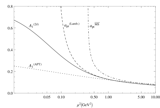
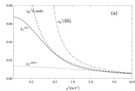
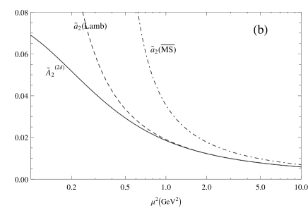
Figure 1 shows the analytic running couplings of the 2anQCD model and APT, at positive low values of (), for the central input values. For comparison, the pQCD couplings in the Lambert renormalization scheme (the scheme of 2anQCD, ) and in the four-loop scheme (at ) are included. Figure 2(a) shows the higher couplings and , and Fig. 2(b) the logarithmic derivatives and , which are defined in Eqs. (71) and (74) in Appendix A. In APT the coupling was constructed according to Eq. (2), and in the 2anQCD model according to Eq. (75a) truncated at the term.
These figures show that the analytic couplings in the infrared regime, in comparison with the pQCD couplings, are very suppressed in (F)APT, and less so in the 2anQCD model.121212 Figure 2(b) shows that the logarithmic derivatives and in the Lambert scheme are almost indistinguishable from each other at , this being the consequence of the construction of the 2anQCD model: for . Namely, application of to this relation implies . On the other hand, Fig. 2(a) shows that the difference between and is significant even up to , this being the consequence of the aforementioned truncation at in the construction of (Appendix A).
The 2anQCD model has been successfully applied anOPE in the analysis of -decay data via Borel sum rules with OPE.
III Perturbation expansion for heavy ground state energy
III.1 General formulas
The analysis of nonrelativistic potential is the starting point for the determination of the ground state energy of and thus of the mass of such systems. The main input in these calculations is the mass (here denoted simply as ), also called quark mass. The masses of the heavy quarkonia [ when , when ] are well measured, and this allows us to extract the corresponding mass . By evaluating an observable, such as the quark-antiquark binding energy here, within anQCD models, at least part of the (chirality-conserving) nonperturbative effects get included in the leading-twist term via the analytization, such as Eqs. (2)-(3) in (F)APT, and (21) in general analytic QCD models.
The coefficients in the (leading-twist) perturbation expansion of the ground state binding energy (i.e., with: and ) of heavy quarkonium in powers of were obtained up to all terms in Ref. PinYnd , the terms in Ref. BPSV , and all terms up to (including logarithmic) are given in Ref. Penin:2002zv . The last term () is now completely known since the parameter from the static potential is now known, Refs. Smirnov:2009fh ; Anzai:2009tm . The general structure of the (leading-twist term of the) ground state binding energy in pQCD is
| (22) | |||||
where
| (23) |
is the (square of the) renormalization scale, is the pole mass of the quark, and the coefficients can be obtained by combining the results of the mentioned literature; cf. Appendix B. The typical scale of the process is a soft reference scale (), which is a typical quark-antiquark momentum transfer inside the quarkonium () and can be fixed by convention. The soft renormalization scale can then be varied around
| (24) |
The quarkonium mass is then
| (25) |
In principle, the input quantity here could be the quark pole mass . However, this mass , in contrast to the mass , suffers from the strong infrared renormalon ambiguity (at Borel parameter value , ). This ambiguity must cancel in the physical sum [Eq. (25)].
It is more convenient to use as input a renormalon ambiguity-free input mass, such as , and we will do this.
In the case of the bottom quark, before we relate the pole mass with the mass , at renormalization energies where (and where the charm quark mass is considered zero, i.e., decoupled), the effects of the nonzero massa have to be subtracted, and they are Brambilla:2001qk
| (26) |
These effects were calculated in Ref. Brambilla:2001qk in pQCD, at the hard renormalization scale . We checked that they do not get significantly modified in APT and in the 2anQCD model.
The pole mass and the mass are then related via the relation
| (27) |
where is zero when , and is given by Eq. (26) when
| (28) |
The coefficient was obtained in Ref. Tarrach:1980up . Also the coefficients , and are known (Refs. Gray:1990yh , Chetyrkin:1999ys ; Chetyrkin:1999qi ; Melnikov:2000qh , respectively) they are given in Eqs. (93) in Appendix C, and in these coefficients is the number of flavors of quarks lighter than . Specifically, the values are: and for ; and and for . On the other hand, in Appendix C we estimate the values of to a reasonably high level of precision (with less than 4 % uncertainty) by a method which uses the structure of the leading infrared renormalon (at ) of the quantity : , .
While the relation (27) is written here at the “hard” renormalization scale , it is straightforward to reexpress the sum on the right-hand side of Eq. (27) at a different, lower, scale . In Appendix C this reexpression is presented explicitly, under the assumption that during the lowering of the scale, , we do not cross the quark threshold. The goal is to express in the perturbation expansion of the binding energy (22), where the renormalization scale is soft, the pole mass via the mass , and for this we need the relation (27) at the soft renormalization scale. It turns out that for the system the hard scale is GeV, i.e., the scale where ; and the soft scale, Eq. (24), is GeV, i.e., the scale where it is more reasonable to expect .131313 Usually, the quark thresholds are taken at . In the case of transition, this is about GeV, above the soft scale of the system. In this case, we take into account also the (three-loop) quark threshold transition at , Ref. CKS . We thus obtain the relation (27) reexpressed at the soft scale of Eq. (24)
| (29) |
Further, the renormalization scheme can also be varied in this relation and in the relations (22)-(23), i.e., the changes of the scheme parameters () from the usual scheme to other schemes affect correspondingly the values of the coupling and of the coefficients. We recall that in (F)APT the chosen scheme here is ; in the 2anQCD model and in Lambert pQCD, the scheme is and for . The relationship between ’s at two different scales and in two different renormalization schemes is summarized in Appendix D, where we also summarize the (three-loop) connection of ’s across the quark threshold.
After performing all these transformations, we can rewrite the original expansion (22) for in terms of the mass, with the coupling at any soft renormalization scale and in any chosen renormalization scheme ()
| (30) | |||||
where ( being the soft renormalization scale parameter), and the logarithm contains now mass
| (31) |
We note that the new (renormalon-ambiguity-free) mass which appears naturally in this expansion is not exactly the mass , but rather
| (32) |
where is given by Eq. (26) when .
The mentioned soft “process scale” () can be regarded, at least formally, to be a variable complex scale. Therefore, the binding energy is, formally, a spacelike observable analytic in ; and the dependence on the renormalization scale parameter disappears when the number of terms in the expansion is infinite. The analytization of of Eq. (30), according to Eqs. (21) [or, in (F)APT: Eqs. (2)-(3)], then leads to
| (33) | |||||
where we use, for simplicity, the notation of Eq. (78) with Eq. (74) for ’s ( integer now) [in (F)APT: Eq. (2)], and denote by the following:
| (34) |
Here, , therefore faster than when , by asymptotic freedom.
The relation (29) in its analytized form is
| (35) |
Since this relation includes at its highest order the term (), in general analytic QCD it is consistent to use in Eq. (35) for the expressions () those given in Eq. (78) [or: Eqs. (75)] with the sum there truncated at (and including) (). On the other hand, the expression (33) for the binding energy includes at its highest order the terms (more precisely, ), therefore it is consistent to use there for the expressions () those of Eq. (78) [or Eqs. (75)] with the sum truncated at (and including) , and expressions of Eq. (79) truncated at (and including) (), where .
The mentioned soft reference scale () can be fixed in pQCD, by convention, by the condition that all the logarithmic terms in the expansion (30) disappear
| (36) |
where is defined in Eq. (32). This type of condition, in analytic QCD, would correspond to fixing the soft reference scale by requiring , for various ’s and . This fixing is not unique since it depends on and . Our convention will be that the leading logarithmic term in Eq. (33) is zero at such scale
| (37) |
It will turn out that this condition has a solution in the case of () in the 2anQCD model, but not in in that model, and not in any case of the (F)APT model. In such respective cases, we will use simply the following simpler analogs of the pQCD condition (36):
| (38) | |||||
| (39) |
These measures of the typical momentum scale of the (nonrelativistic) quark inside the quarkonium are rather low, GeV in , and GeV in . In pQCD such scales are problematic, because they are not far away from the unphysical (Landau) singularities of ; in analytic QCD models, no such problems appear in principle.
III.2 Separation of the soft and ultrasoft contributions
The pole mass and the static potential both contain the leading infrared renormalon () singularities, and cancellation of these singularities takes place in the sum Hoang:1998nz ; Brambilla:1999xf ; Beneke:1998rk . As a consequence, this cancellation must take place also in the quarkonium mass Kiyo:2000fr ; Brambilla:2001fw ; Brambilla:2001qk ; Pineda:2001zq ; Lee:2003hh ; Contreras:2003zb , more specifically, in the sum where [] is the soft part of the binding energy , and denotes the (ground) state of the quarkonium. The typical soft distance in the quarkonium is , where or . Since , we have . This leads to the so called “power mismatch” in the renormalon cancellation in the pQCD expansion of the sum Hoang:1998ng (see also: Kiyo:2000fr ): the terms in tend to cancel numerically the terms in . Therefore, since the binding energy is now known up to , it is very convenient to have the relation up to , i.e., to have a good estimate for the coefficient and to use it, so that the effects of renormalon cancellation in can be seen numerically more clearly. This was the main reason for performing the analysis in Appendix C resulting in estimates of , Eq. (105). This cancellation, term by term, should be numerically more precise (at sufficiently high orders) if the renormalization scales used in and in [Eqs. (29) and (30)] are taken to be equal. This renormalon cancellation will be our guiding principle for the separation of the soft () and the ultrasoft () part in the binding energy
| (40) |
Typical scales are , and the part of the binding energy is . We can parametrize the - separation by a dimensionless parameter such that the - factorization scale is written as
| (41) |
where is a (chosen) reference scale. It is expected that usually , but it does not have to be so always. The part can be rewritten, in terms of as (cf. Ref. Contreras:2003zb )
| (42) |
and in analytic QCD correspondingly
| (43) |
where is a renormalization scale (), and the two coefficients are
| (44) |
The expansion of the soft () part of the binding energy is then, according to Eq. (40), the same as the expansions (30) and (33), with the exception of the replacements141414 The coefficients and , representing the leading part of the (quasi)observable , are renormalization scale () and scheme independent. of two coefficients and
| (45) |
The - factorization, i.e., the parameter , will then be determined, in each model, by requiring that the leading infrared renormalon cancellation in be exact at the last available order, i.e., that the term in and the term 151515 The latter term includes all terms (). in cancel exactly.
The part of the quarkonium mass, , will be evaluated in each case according to a procedure which takes into account those problems of low-scale evaluations which appear in the considered model (2anQCD, pQCD, (F)APT).
We recall that the binding energy is a Euclidean quantity because it depends on spacelike quark-antiquark momentum transfer (). Analytization of such quantities must follow the procedure (21). On the other hand, the quark pole mass is a Minkowskian quantity because it depends on the timelike pole momentum (). We note that our analytization procedure for the quark pole mass is again the procedure (21): in the relation (27) [and then reexpressing via ’s at a lower soft scale , for renormalon cancellation]. This procedure, for the Minkowskian quantities, is analogous to the fixed order perturbation theory (FOPT) in pQCD, Ref. BeJa , where the couplings in the corresponding contour integral, on the contour , are Taylor-expanded around the spacelike point . As a result, the kinematic -terms appear in the expansion coefficients .
Another analytization of the pole mass expansion would involve contour integration of the corresponding Euclidean quantity with (exact) RGE-running couplings along the contour, cf. Ref. CKSir . This procedure is analogous to the Contour Improved Perturbation Theory (CIPT) in pQCD; in such a case, the aformentioned terms are effectively resummed, Refs. RKP ; KK . We decided not to pursue this CIPT type of analytization, because it is technically more demanding due to the additional running of the mass factor ; and because in this approach the renormalon cancellation mechanism, due to the mentioned resummations, probably changes its practical form. This problem remains to be addressed in the future.
IV Numerical results
IV.1 Bottom mass extraction
In this section, we extract from the mass of quarkonium the mass in (F)APT, 2anQCD model, and in pQCD in two renormalization schemes ( and in the Lambert scheme of 2anQCD). For this, we use the relation between and the well-measured mass of the quarkonium PDG2010
| (46) |
The dependence on the (soft) renormalization scale in the pole mass and in the soft binding energy occurs due to the truncation of the series for these two quantities. For the same reason, the ultrasoft binding energy has strong dependence on the ultrasoft renormalization scale () due to the drastic truncation of this quantity at its leading order (). As mentioned in the previous Section, the separation of the and parts of the binding energy will be performed here by determining the - separation parameter , Eqs. (40)-(45), by the requirement of cancellation of the leading renormalon in .
In contrast to the other three models, (F)APT gives a very small central value for the - separation parameter . This reflects the difficulty in the (F)APT scenario to exactly enforce the leading renormalon cancellation of the term of with the corresponding term of . If, on the other hand, we impose in (F)APT the condition , more specifically the central value and variation in the interval , the results change somewhat, the central extracted value of increases by about GeV, and the absolute values of the part of the binding energy and of various other uncertainties of get reduced. We will consider in (F)APT only the natural range of the - separation parameter, , rather than the exceedingly small values of required by the exact renormalon cancellation. In the other three models (2anQCD, and in Lambert and pQCD), the renormalon cancellation is imposed without any problems, resulting in the values of within the interval between and .
In the previous section we mentioned that we take for the number of active flavors in the binding energy, i.e., in this case the mass is considered to be infinite (decoupled). It turns out that, while the effects of the finiteness of cannot be neglected in the relation between and , Eqs. (26)-(27), these effects can be safely neglected in the binding energy ; cf. Ref. Brambilla:2001qk based on Refs. Gray:1990yh ; Eiras:2000rh ; Hoang:2000fm .
Application of the formalism described in Secs. II.1 and II.2 (with Appendix A) for the calculation of the couplings of the analytic QCD models (F)APT and 2anQCD, and in Sec. III for the calculation of , and in terms of these couplings, then gives us the following results:
| (47h) | |||||
| (47i) | |||||
| (48j) | |||||
| (48k) | |||||
We will comment on the above uncertainties below. For completeness, we give here also the results of the same kind of analysis in pQCD, first in the Lambert renormalization scheme (i.e., the scheme as used in 2anQCD: , for ); and in the (four-loop) scheme:
| (49j) | |||||
| (49k) | |||||
| (50j) | |||||
| (50k) | |||||
The value of the - separation parameter was determined in all cases by the aforementioned renormalon cancellation in the sum , except in the (F)APT case, as discussed above. Below we present these resulting sums, for the central choices of the aforementioned four results, where we combine in each parenthesis the (positive) terms of and the corresponding (negative) terms of (), in order to see more clearly the tendency of the renormalon cancellation; the part is given separately
| (51a) | |||||
| (51b) | |||||
| (52a) | |||||
| (52b) | |||||
| (53a) | |||||
| (53b) | |||||
| (54a) | |||||
| (54b) | |||||
We can see from Eqs. (51a)-(54a) explicitly that for the chosen corresponding central values of the parameter the renormalon cancellation is exact in the last term [the fifth term, named ] in the sum for the soft mass , except in the case of (F)APT where was chosen and the cancellation in is approximate.
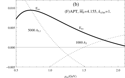
The extracted values of , Eqs. (47)-(50), have a strong uncertainty coming from the ultrasoft () regime and from the related separation. The origin of this uncertainty lies in the strong dependence of the binding energy on the renormalization scale and on the - separation parameter , cf. Eqs. (41)-(44). The behavior of the binding energy in the three models (2anQCD, and pQCD in the two schemes), as a function of the renormalization scales in the low-momentum regime, is presented in Fig. 3(a), and in the case of (F)APT in Fig. 3(b).
In the 2anQCD model and in pQCD, we do not consider the scales below GeV, because at GeV the coupling ( in our approach)161616 We recall that in the 2anQCD model we calculate in the couplings as sums of with ; and in [and ] the couplings [and ] as (derivatives of the) sums of [and ] with ; cf. discussion in Sec. II.2, Appendix A, and Sec. III. in the 2anQCD model reaches a local maximum, indicating that the model may not necessarily give reliable values of and below such scales. Therefore, in general, we will not consider lower than 1.1 GeV, in the 2anQCD model and in pQCD. in 2anQCD reaches a local minimum at slightly above 1.1 GeV. Therefore, we estimate the part of the binding energy in the 2anQCD model in the following way [we use the notation ]:
| (55) |
where the soft reference scale was determined by the condition (37), and gave for the central values of the input parameters ( and of the second line of Table 1; ; GeV) the soft reference scale value GeV.
In the two pQCD approaches, decreases monotonously when decreases below the soft reference scale of Eq. (36). For pQCD in the Lambert scheme (), with central values of the input parameters, the soft reference scale turns out to be GeV, and the binding energy at GeV reaches the value of GeV. In the scheme, however, GeV, which is exceedingly low and indicates failure of the method already at such scales, due to vicinity of Landau singularities of the running coupling.171717 It turns out that the Landau cut in the perturbative coupling starts in the four-loop () scheme already at about GeV. In the Lambert scheme [Eq. (16) with the central value ] there is one pole at GeV; the cut begins at an even lower value GeV. The 2anQCD coupling has, of course, no Landau singularities (poles and cuts), although it almost coincides with the Lambert pQCD coupling at higher scales , Ref. 2danQCD . Therefore, in we take as the minimal acceptable scale GeV, where GeV (and GeV) when the central values of the input parameters are used. Thus, in pQCD we estimate the binding energy as
| (56) |
with GeV and GeV in the Lambert and schemes, respectively.
In the (F)APT case, on the other hand, is fixed according to Eq. (39) and gives, for the central input parameter values, the value GeV. In (F)APT no practical problems appear at scales GeV. reaches a moderate maximum value of GeV at GeV for the chosen central value . Therefore, we estimate the part of the binding energy in (F)APT in the following way:
| (57) |
In Eqs. (47)-(50), the uncertainties in originating from these determinations of the binding energy are denoted by the subscript .
The related uncertainties for the extracted values of originate from the variation of the - separation parameter , and are denoted by the subscript in Eqs. (47)-(50). The parameter was varied in such a way that the last [fifth, ] term in the series for the soft mass [cf. Eqs. (51a)-(54a)] varies between the penultimate term of these series, and its negative , these two cases correspond to the upper and the lower entry of uncertainty of , respectively. In the (F)APT case the exact renormalon cancellation was not achieved and the parameter was varied between 0.1 and 10, i.e., .
The other uncertainty in the determination of comes from the uncertainty of the scale. In (F)APT it comes from GeV and is denoted by the subscript in Eq. (47h). In the 2anQCD model and in the two pQCD approaches (the Lambert scheme and scheme), this uncertainty comes from PDG2010 and is denoted by the subscript in Eqs. (48j), (49j), and (50j).
Yet another uncertainty of , in the 2anQCD model and in Lambert scheme pQCD, comes from the variation of the (Lambert) renormalization scheme parameter , cf. Table 1 and Eqs. (16)-(18). and is denoted in Eqs. (48j) and (49j) by the subscript . The scheme in (F)APT was fixed by the underlying pQCD solution, Eqs. (9)-(10): , i.e., effectively the two-loop solution.
The uncertainty due to the variation of the soft renormalization scale was denoted in Eqs. (47)-(50) by the subscript . We varied around the central value of the soft reference scale, between and . The scale is determined by Eqs. (36), (37) and (39) in pQCD, 2anQCD and (F)APT, respectively, for central values of the input parameters , , etc.
Finally, the uncertainty GeV due to nonzero mass [Eq. (26; cf. also Eqs. (29)-(32)] results in the uncertainties GeV of , denoted in Eqs. (47)-(50) by the subscript .
We see in Eqs. (47)-(50) that the largest resulting uncertainty in the determination of is the one originating from the uncertainty of the determination of the binding energy (except in (F)APT where values are small). These uncertainties are larger in the two pQCD approaches, due to the influence of the nearby (unphysical) Landau singularities in the running couplings. The contribution of the regime to the quarkonium mass, in the 2anQCD model and in pQCD, increases the predicted value of . This is so because the binding energies are in these cases significant and negative; cf. also Fig. 3(a). If we had ignored the existence and separation of the contributions, i.e., if we had used in the entire binding energy simply a common soft renormalization scale , the predicted values of in the 2anQCD model and in Lambert and pQCD would have decreased, by , , and GeV, respectively, as can be deduced from the -origin uncertainties in Eqs. (48j)-(50j). On the other hand, in (F)APT the choice would only slightly increase the central value of , by GeV [cf. Eq. (47h)], basically because the values of in (F)APT are much smaller; cf. Fig. 3(b).
For better visibility, we present the results for the central extracted values of of the aforementioned four models in Table 2, and for various uncertainties in Table 3.
| model | ||||||
|---|---|---|---|---|---|---|
| (F)APT | 1.000 | 1.596 | 9.454 | 0.006 | ||
| 2anQCD | 0.238 | 2.084 | 9.815 | -0.355 | ||
| pQCD Lamb. | 0.306 | 1.729 | 9.816 | -0.355 | ||
| pQCD | 0.248 | 1.869 | 10.078 | -0.617 |
| model | () | () | ||||||
|---|---|---|---|---|---|---|---|---|
| (F)APT | +0.002 | +0.005 | (1.0+9.0) | -0.019 | – | (–) | -0.004 | -0.005 |
| -0.002 | -0.004 | (1.0-0.9) | +0.020 | – | (–) | +0.002 | +0.005 | |
| 2 an- QCD | -0.068 | +0.015 | (0.238-0.100) | -0.005 | -0.023 | (-4.76+2.66) | +0.017 | -0.005 |
| +0.071 | -0.016 | (0.238+0.173) | +0.005 | +0.034 | (-4.76-0.97) | -0.025 | +0.005 | |
| pQCD Lamb. | -0.091 | -0.013 | (0.306+0.194) | +0.010 | +0.027 | (-4.76+2.66) | -0.002 | -0.005 |
| +0.097 | +0.017 | (0.306-0.119) | -0.010 | -0.008 | (-4.76-0.97) | -0.041 | +0.005 | |
| pQCD | -0.177 | -0.082 | (0.248+0.642) | +0.031 | – | (–) | -0.004 | -0.005 |
| +0.200 | +0.084 | (0.248-0.181) | -0.027 | – | (–) | -0.075 | +0.005 |
We wish to address here briefly the question of nonperturbative (NP, higher-twist) contribution to the quarkonium mass. In the heavy quark system such as , the NP contribution can be estimated, and in the leading order it comes from the gluon condensate and is given by Voloshin:hc
| (58) |
The factor in (four-loop) pQCD is unreliable for realistic scales GeV, due to the vicinity of the Landau singularities (cf. footnote 17). In the 2anQCD model, for purposes of estimation, we replace by or by . In the interval we have ; the couplings and cover in this interval the values between and . For these values, and using the central value of the gluon condensate Ioffe:2002be (cf. also Refs. Ioffe and anOPE ), and for GeV, we obtain the following estimate:
| (59) |
This effect is relatively small and has large uncertainties. If we take it into account, then the central extracted values of in this subsection decrease somewhat, the decrease being GeV.
We wish to comment briefly on the following aspect: the results of this subsection show that the extracted values and various uncertainties are similar in the 2anQCD model and the corresponding Lambert pQCD. The main reason for this lies in the fact that the scheme parameters (, ) are the same in both frameworks, and that the two corresponding running couplings practically merge at high momenta : . Nonetheless, the evaluation methods for these two cases differ somewhat due to the different types of truncations involved. In pQCD, the quantities and were calculated as truncated series of powers , truncated at and , respectively. In the 2anQCD model, they were effectively calculated as series in logarithmic derivatives , truncated at and , respectively; namely, the analytic power analogs in were evaluated as a series in ’s up to , and in as a series in ’s up to (cf. Appendix A).
For comparison, we present in Table 4 a list of extracted values of (and ) by various methods in the literature: lattice calculations, sum rules (pQCD+OPE), and from meson spectra (pQCD). The latter pQCD calculations account for the renormalon cancellation, but most of them either do not consider the ultrasoft contributions, or they include them unseparated from the soft contributions (using the same scale in the soft and the ultrasoft).
| reference (year) | method | (GeV) | (GeV) |
|---|---|---|---|
| ETM (2011) Dimopoulos:2011gx ; Blossier:2010cr | lattice () | (Dimopoulos:2011gx ) | (Blossier:2010cr ) |
| GST (2008) Guazzini:2007ja | lattice (quenched) | – | |
| DGPS (2006) Della Morte:2006cb | lattice (quenched) | – | |
| DGPTP (2003) deDivitiis:2003iy | lattice (quenched) | ||
| Narison (2011) Narison:2011xe | sum rules | ||
| HPQCD (2010) McNeile:2010ji | sum rules181818 Uses sum rules with lattice input. | ||
| CKMM et al. (2009) Chetyrkin:2009fv | sum rules | ||
| PS (2006) Pineda:2006gx | sum rules | – | |
| BCS (2006) Boughezal:2006px | sum rules | ||
| LKW (2011) Laschka:2011zr | spectrum | ||
| CCG (2003) Contreras:2003zb | spectrum | – | |
| Lee (2003) Lee:2003hh | spectrum | – | |
| BSV (2001) Brambilla:2001qk | spectrum | – | |
| Pineda 2001 Pineda:2001zq | spectrum | ||
| This work | spectrum | ((F)APT) | ((F)APT) |
| (2anQCD) | (2anQCD) | ||
| (pQCD Lamb.) | (pQCD Lamb.) | ||
| (pQCD ) | (pQCD ) |
We can see that (F)APT results agree with those of the usual pQCD calculations of the quarkonium spectrum and those of the sum rules (pQCD+OPE). The 2anQCD results are incompatible with those results, but are compatible with the results of lattice calculations. The same can be claimed for the estimates of our pQCD approach (in the Lambert and schemes), but the uncertainties there, coming principally from the ultrasoft sector, are larger, especially in scheme.
IV.2 Charm mass extraction
In this case, , and the quarkonium mass is now GeV PDG2010 . We basically repeat the analysis as in the case of . There are some differences, though:
- •
-
•
The typical soft reference scales [Eqs. (36) and (38)] are now significantly lower: GeV or even lower (in the case we had: GeV). This, in conjunction with our suggestion that the considered models 2anQCD and pQCD (in the Lambert and schemes) are not necessarily to be trusted at scales below GeV, implies that the typical soft renormalization scales should be chosen significantly higher than . We choose in these three models. In this case, the lowest possible soft scale, is slightly above GeV. In (F)APT, the soft renormalization scale will also be varied in this way, giving, however, somewhat lower central value for the renormalization scale:, GeV.191919 If we used in (F)APT a lower definition of the central renormalization scale, ( GeV), the predicted central value of would go up by only GeV. The scale variation results in small uncertainties of the extracted mass , but these uncertainties may be underestimated because .
-
•
In general, the cancellation of the leading renormalon now implies for the - separation parameter such values for which the absolute values of are significantly smaller than in the case, and consequently, the ambiguities are smaller. Since we now use for the central choice of the soft renormalization scale , is calculated in the 2anQCD model and in pQCD in the following way:
(60) where the soft reference scale in the 2anQCD model is determined by Eq. (38)202020 Note that in the 2anQCD model in the case the condition (37) cannot be fulfilled. and in pQCD by Eq. (36). In (F)APT, we do not have practical problems at low scales GeV, and the energy as a function of low scale turns out to have a moderate local maximum and a moderate local minimum; hence we use
(61) where these values are quite small: in the central case (, ), the local maximum is GeV and is reached at GeV, and the local minimum is GeV and is reached at very low scale GeV [cf. Fig. 4(b)].
-
•
The exact renormalon cancellation requirement in (F)APT gives again an exceedingly small value of the - separation parameter, . In (F)APT we vary the parameter again around its central chosen value , in the interval between and , just as it was done in the case of (F)APT.
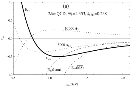
The described behavior of the in the analytic 2anQCD model and in pQCD in the two schemes, as a function of the ultrasoft scales , is presented in Fig. 4(a), and in the case of (F)APT in Fig. 4(b).
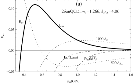
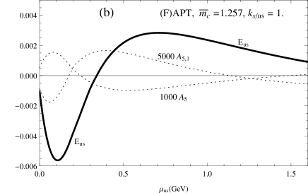
Comparing Figs. 4(a) and (b), we see that - GeV in the 2anQCD model, and GeV in (F)APT. Furthermore, comparing with the corresponding curves in Figs. 3(a) and (b) for the , we can see that in the 2anQCD model and in the two pQCD approaches, the absolute values are by almost two orders of magnitude smaller than , principally because the renormalon cancellation gives us in the two cases significantly different - separation parameter values: and . Further, the values of (for ) in pQCD are larger than in the 2anQCD model, especially in pQCD. In the (F)APT case, the values of () are quite small, being in case smaller by almost one order of magnitude. All this is reflected also in the numerical results of this and of the previous subsection.
The resulting extracted values of are
| (62a) | |||||
| (62b) | |||||
| (63e) | |||||
| (63f) | |||||
| (64e) | |||||
| (64f) | |||||
| (65e) | |||||
| (65f) | |||||
In order to see more clearly the renormalon cancellation, we present below, as in Sec. IV.1, the sum for the soft mass , combining in each parenthesis the (positive) term from and the (negative) term from the soft binding energy (), for the central input values of parameters , () and ; separately we present below also .
| (66a) | |||||
| (66b) | |||||
| (67a) | |||||
| (67b) | |||||
| (68a) | |||||
| (68b) | |||||
| (69a) | |||||
| (69b) | |||||
As in the previous subsection in the case of , we present now for the case , for better visibility, the results for the central extracted values of of the four models in Table 5, and for various uncertainties in Table 6.
| model | ||||||
|---|---|---|---|---|---|---|
| (F)APT | 1.00 | 1.004 | 3.098 | -0.001 | ||
| 2anQCD | 4.06 | 1.422 | 3.087 | +0.010 | ||
| pQCD Lamb. | 5.59 | 1.382 | 3.083 | +0.013 | ||
| pQCD | 3.08 | 1.585 | 3.131 | -0.034 |
| model | () | () | |||||
|---|---|---|---|---|---|---|---|
| (F)APT | -0.002 | -0.002 | (1.0+9.0) | -0.011 | – | (–) | -0.002 |
| +0.002 | +0.002 | (1.0-0.9) | +0.011 | – | (–) | +0.002 | |
| 2dan- QCD | +0.003 | +0.007 | (4.06-3.61) | -0.005 | -0.014 | (-4.76+2.66) | -0.002 |
| -0.003 | -0.007 | (4.06+39.5) | +0.005 | +0.003 | (-4.76-0.97) | +0.005 | |
| pQCD Lamb. | +0.001 | +0.021 | (5.59-5.355) | -0.004 | 0.000 | (-4.76+2.66) | -0.003 |
| -0.001 | -0.022 | (5.59+148.4) | +0.004 | 0.000 | (-4.76-0.97) | +0.015 | |
| pQCD | -0.011 | +0.066 | (3.08-2.86) | -0.002 | – | (–) | -0.003 |
| +0.011 | -0.075 | (3.08+66.9) | +0.002 | – | (–) | +0.017 |
The nonperturbative (NP) contribution coming from the gluon condensate, cf. Eq. (58) for the system in the previous subsection, is unreliable for the lighter system, since the next-to-leading corrections are in this case large and tend to make the result unreliable, cf. Ref. Pineda:1996uk .
Comparing the results for in this subsection with those for in the previous subsection, we see that the soft-ultrasoft separation parameter in the 2anQCD model and pQCD is now larger: -, while in case we had -. This is a consequence of the requirement of the leading renormalon cancellation. As a result, the ultrasoft contributions to the mass are by an order of magnitude smaller (in absolute value) than those to the mass, surprisingly. The extracted values of thus suffer from less (ultrasoft) uncertainty than the extracted values of . On the other hand, in (F)APT, the ultrasoft sector is always suppressed, a consequence of the suppressed (F)APT couplings in the infrared.
The extracted values of obtained in this work, in all four models, are compatible with all those obtained in the literature (from lattice, sum rules, and spectrum calculations), as can be seen from Table 4.
V Summary
We evaluated, in two analytic QCD models and in perturbative QCD (pQCD, in two schemes), the quark-antiquark binding energies (up to ) and masses of ground state quarkonia (), as functions of the quark mass [], also called the quark mass. In analytic QCD models the QCD running coupling has no unphysical (Landau) singularities in the plane.
The use of the analytic QCD models was motivated by the fact that the typical soft () momentum scales in the ground bound states of quarkonia are low ( GeV and GeV, for and , respectively), and that the typical ultrasoft () momentum scales are even lower. This, in conjunction with the fact that Landau singularities of the pQCD coupling reach relatively high momenta: GeV in the usual (four-loop) scheme (with ), and GeV in the Lambert scheme (). So we can apply in analytic QCD generally more natural renormalization scales at which the pQCD couplings are sometimes “out of control.”
One analytic QCD model applied here was the Analytic Perturbation Theory (APT) of Shirkov, Solovtsov, Solovtsova, and Milton et al. (Refs. ShS ; MSS ; Sh1 ; Sh2 ), which has been extended by Bakulev, Mikhailov and Stefanis to the Fractional Analytic Perturbation Theory (FAPT) for calculation of the fractional power analogs (Refs. BMS1 ; BMS2 ; BMS3 ). (F)APT can be regarded as a model with minimal analytization of pQCD in the conceptual sense. Namely, it keeps the perturbative discontinuity function unchanged on the entire positive- semiaxis, while removing the (perturbative) discontinuity at in order to ensure the analyticity of . It thus contains no additional regulators in the positive low- regime. One of the strengths of (F)APT is that it has as a parameter only the pQCD-type scale; i.e., it contains no new parameters. As a result, it has finite coupling at , and at . The latter means that it behaves somewhat differently from the underlying pQCD (with the same ) even at high squared momenta . The value of the scale is adjusted so that the high- QCD phenomenology is reproduced.
The other analytic QCD model applied here was the two-delta analytic QCD model (2anQCD), Refs. 2danQCD ; anOPE . This model can be regarded as a model with minimal analytization of pQCD in the numerical sense. Namely, in this model the behavior of the discontinuity function in the unknown low- regime ( GeV) is parametrized (with two deltas) in such a way that: (a) at the model becomes practically indistinguishable from the (underlying) pQCD, ; and (b) the measured value of the semihadronic strangeless decay ratio of the lepton (the hitherto best measured inclusive low-energy QCD observable), , is reproduced. These conditions fix most of the mentioned low- regime parameters. The value of the scale is the same as in the (underlying) pQCD, so that the high- QCD phenomenology is reproduced. In contrast with (F)APT, in the 2anQCD model one relevant parameter remains variable, namely the parameter (), which we vary in the phenomenologically viable interval, i.e., approximately .
The main conclusions of this work are the following: analytic QCD approaches which at high energies follow the pQCD behavior closely (such as the 2anQCD model) indicate that the ultrasoft regime in the quarkonium () is important. Our approach, together with the leading renormalon cancellation condition, gives us clues about how to estimate the effects of the ultrasoft regimes in pQCD. In both the 2anQCD model and in pQCD we obtain, as a consequence, extracted values of which are significantly higher ( GeV) than most of those ( GeV) obtained in the sum rule approaches (which use pQCD+OPE) and in the usual pQCD calculations of meson spectra. These approaches usually either do not include the ultrasoft contributions, or they include them unseparated from the soft contributions (i.e., the ultrasoft and soft scales are set to be equal). As an additional consequence, the uncertainties in the extracted values of in our approach are dominated by the ultrasoft sector and are, especially in pQCD in the scheme, larger than in the usual pQCD approaches. Further, the extracted values of in the 2anQCD model, GeV, are compatible with those of lattice calculations; cf. Table 4. On the other hand, the 2anQCD model indicates that the ultrasoft regime in the quarkonium () is less important, principally because the leading renormalon cancellation condition results in smaller ultrasoft coefficients in this system. The extracted values, GeV, are compatible with those of pQCD (or pQCD+OPE) approaches, and those of the lattice calculations. On the other hand, the (F)APT of Shirkov et al., suppresses the infrared contributions because the higher order couplings in (F)APT are more strongly suppressed in the infrared than the 2anQCD couplings. The extracted values in (F)APT, GeV and GeV, are compatible with those obtained from the sum rules and from the usual pQCD spectrum calculations.
Acknowledgements.
We thank A. Pineda for useful comments. C.A. thanks Bogolyubov Laboratory of Theor. Physics, of the Joint Institute for Nuclear Research, Dubna, for warm hospitality during part of this work. C.A. further thanks J. Otálora for help in using calculational software. This work was supported in part by MECESUP2 (Chile) Grant FSM 0605-D3021 (C.A.), and by FONDECYT (Chile) Grant No. 1095196 and Anillos Project ACT119 (G.C.).Appendix A Analytic analogs of powers and of terms in general analytic QCD models
We consider that a (general) anQCD model is defined via an analytic analog of in ther complex plane, or, equivalently, by the discontinuity function [] on the positive semiaxis .
For such general anQCD models, the higher order couplings [analogs of ] were constructed in Refs. CV1 ; CV2 for integer , and Ref. GCAK for general (noninteger) . Below we will summarize the basic aspects of such construction.
Since the general anQCD models, with the exception of APT, have at low () different discontinuity function than the pQCD coupling , we cannot use the (F)APT method [Eq. (3)] for the construction of the analytic analogs of . The analogs of the integer powers in such general models were constructed in Refs. CV1 ; CV2 , where it was shown that it is imperative to construct first the analogs of the logarithmic derivatives of in the following way:212121 If the analytization is performed in any other way, the renormalization scale and scheme dependence of the resulting truncated analytic series of any observable will in general increase (instead of decrease) when the number of terms in the series increases; cf. CV1 ; CV2 .
| (70) |
In pQCD, the logarithmic derivatives
| (71) |
are related with the powers of in the following way (using RGEs in pQCD):
| (72a) | |||||
| (72b) | |||||
| (72c) | |||||
This means that the powers of are linear combinations of logarithmic derivatives
| (73a) | |||||
| (73b) | |||||
| (73c) | |||||
These relations, in conjunction with the analytization Eq. (70), imply that the analytic analogs of powers , in general anQCD models, can be expressed as linear combinations of the logarithmic derivatives
| (74) |
in the following form:
| (75a) | |||||
| (75b) | |||||
| (75c) | |||||
In Ref. GCAK this analytization was extended to the case when is noninteger222222 This relation was also reformulated so as to be applicable in a larger interval: ; cf.Eq. (22) of Ref. GCAK .
| (76) |
where, as always, , and is the polylogarithm function.232323 In Mathematica Math8 it is implemented under the name PolyLog. The corresponding analogs of powers are then obtained by using the general relations
| (77) |
and the linearity of analytization, i.e.
| (78) |
The coefficients , for general real and positive integer , were calculated in Ref. GCAK , and are combinations of gamma functions and their derivatives, with arguments involving ( being various integers).
Furthermore, since , the linearity of analytization then implies
| (79) | |||||
where in the terms on the right-hand side we use expressions for obtained by Eq. (76). Comparing Eqs. (79) and (76), we see that the terms in the above sum represent integrals over the scale involving the basic discontinuity function of the model () and derivatives of the polylogarithm function with respect to its index . In the evaluation of the binding energy we will encounter the logarithmic terms of the type (79) with integer (); however, the derivatives with respect to index in Eq. (79) imply that we must know the behavior of around the integer value , i.e., we need to use here the expression (76) for noninteger , or a version of it with improved integration convergence, Eq. (22) of Ref. GCAK (cf. also the earlier footnote 22).
Appendix B Ground state quark-antiquark binding energy
According to Refs. PinYnd ; Chetyrkin:1999qi ; Penin:2002zv , the perturbation expansion of the quark-antiquark binding energy , in terms of the quark pole mass and , is
| (80) |
where
| (81) |
| (82) |
| (83) | |||||
| (84) |
The two contributions to are
| (85) | |||||
| (86) | |||||
The following notations were used:
| (87) | |||||
| (88) |
The RGE coefficients are in the scheme
| (89) |
The constants and are
| (90) | |||||
The value for the constant associated with the three-loop soft contribution was obtained in Refs. Smirnov:2009fh ; Anzai:2009tm and is
| (91) |
where
| (92) |
Appendix C Renormalon-based estimate of coefficient
The term in the expansion of in Eq. (27) can be estimated by a method closely related with the approach presented in Sec. II of Ref. Contreras:2003zb . The pQCD version of the sum in Eq. (27) can be reexpressed in terms of at any other renormalization scale
| (93a) | |||||
| (93b) | |||||
| (93c) | |||||
| (93d) | |||||
| (93e) | |||||
where , while and are the renormalization scheme independent coefficients [given just after Eq. (9)]. Here, is the number of light active flavors (quarks with masses lighter than ).
Since and are explicitly known, the Borel transform is known to order
| (94) |
The function has renormalon singularities at Bigi:1994em ; Beneke:1994sw ; Beneke:1999ui . The behavior of near the leading infrared (IR) renormalon singularity is determined by the resulting renormalon ambiguity of . This ambiguity is a (QCD) scale which, having the dimension of energy and being renormalization scale and scheme independent, must be proportional to the QCD scale : Beneke:1994rs . This scale can be expressed in terms of and ( being any renormalization scale) in the form
| (95) |
where
| (96a) | |||||
| (96b) | |||||
| (96c) | |||||
The above constants, expressed in terms of and of , appear in the expansion of the residue of the Borel transform at the pole
| (97) |
where is analytic on the disk and can be expanded in powers of . The form of the representation (97) is called bilocal and was proposed in Ref. Lee:2003hh . We can assume that the coefficients are known up to , because the coefficient (in the scheme) is known to a large degree by Padé-related methods of Ref. Ellis:1997sb
| (98) |
with , , , , and . This gives for , for , and for . The residue parameter can be determined with high precision by using the idea of Refs. Lee:1996yk , i.e., by calculating (cf. Refs. Pineda:2001zq ; Lee:2003hh ; Cvetic:2003wk ):
| (99) |
where
| (100) |
and the first coefficients in the expansion in powers of of this quantity are known from the known coefficients and . We can use a combination of truncated perturbation series and Padé approximants [1/1] for , as presented in Ref. Cvetic:2003wk , and obtain
| (101) |
with the uncertainties in these values of roughly .
In the bilocal expansion (97), the analytic part can be taken as a polynomial in , i.e., a truncated expansion in powers of . The coefficients of the latter expansion can be related with ’s by equating the expansion of Eq. (97) in powers of with the expansion (94), resulting in
| (102a) | |||||
| (102b) | |||||
where, by convention, . The numbers of Eqs. (96), which enter the sum in Eq. (102b), are known only up to , because, in , only up to are reasonably known ( approximately, as mentioned). For , these values are: , , (and ). For , they are: , , (and ). And for they are: , , (and ). Therefore, the sums in (102b) are truncated at .
Theoretically, the pole closest to the origin in is at , at least in the large- approximation.242424 Nonetheless, there is a possibility that at two-loop order the kinetic term contributes to an IR renormalon at in , cf. Ref. Neubert:1996zy . Since in the coefficients for are known [because and are known], we can construct the Padé and check the pole of it. It turns out that this Padé, at the natural scale , has the pole at , for , respectively, reflecting correctly the theoretical expectation.252525 However, the dependence of this position is rather strong. For example, when varies by 10 % around , the pole position in [1/1] varies between and in the case, between and in the case, and between and in the case. We can extend further this reasoning and obtain the next coefficient (at ) by requiring that the Padé has the pole at . This gives us
| (103) |
If constructing with these values of the other possible Padé approximant of index 3, namely , it turns out that the nearest to origin pole of such Padé is then at for , respectively. This indicates that the obtained values of , Eq. (103), are consistent.262626 We used for the scheme coefficient the estimated values (98), with , for , respectively, from Ref. Ellis:1997sb . Simpler Padé-based estimates of were obtained in Ref. Elias:1998bi : for , respectively (and a large negative and uncertain value for ). The value (for ) in this case differs substantially from the value . If we repeat for the value () the same procedure described above, we obtain (for we got: ); hence the expressions of of Eq. (102b) change, and the pole of becomes (before: ), not close to the theoretical pole . Furthermore, from the requirement that has the pole at we now get (before: ), and using this value of in the Padé we obtain the pole nearest to the origin (before: ). This indicates that the estimate (for ) is not giving results consistent with the theoretical expectations of the renormalon structure of . Using these values, we obtain from the relation (102b) (with the natural choice ) at an estimate for
| (104) |
This gives us numerically the following estimates (we recall that for , , quark, respectively):
| (105) |
The principal origin of the uncertainties in these expressions is the uncertainty in the residue parameter (roughly , i.e., less than 4 %), implying an uncertainty in of a few percent (below 4 %).
An analysis similar to this one has been performed in Ref. Pineda:2001zq . There, however, the term and the coefficients were not included in the analysis. The results of Ref. Pineda:2001zq are: for , respectively. These results are by about - higher than ours [Eq. (105)]. In another approach, applying the effective charge method (ECH) of Refs. ECH to a Euclidean analog of the quantity , an approach using the idea of Ref. KSt extended in Ref. CKSir to the mass-dependent Minkowskian quantities, the authors of Ref. KK obtained for these coefficients the estimates , respectively. These quantities are by about - lower than ours. On the other hand, the corresponding estimates in Ref. CKSir are , respectively.272727 At the time, the coefficient was not known, and the authors of Ref. CKSir used in the estimates of the analogously ECH-estimated values of , respectively (the exact values are ).
Appendix D Variation of pQCD coupling with scales and schemes
In this appendix we give the relation between and , where the latter is expressed as power expansion of the former (cf. Appendix A of Ref. Cvetic:2000mz for details)
| (106) | |||||
where we denote
| (107a) | |||||
| (107b) | |||||
For the purposes of our paper, it is sufficient to consider in the above relation (106) terms up to (including) terms .
The three-loop threshold connection of in the scheme at the threshold scale (where ; usually ) can be written as the following relation between and :
| (108) |
where
| (109) |
and the coefficients were calculated in Ref. CKS
| (110) |
where , and in Eq. (110) is the number of light quark flavors, i.e., in the considered case of transition from to .
References
- (1) M. Peter, Phys. Rev. Lett. 78 (1997) 602 [arXiv:hep-ph/9610209]; Nucl. Phys. B 501 (1997) 471 [arXiv:hep-ph/9702245].
- (2) Y. Schröder, Phys. Lett. B 447 (1999) 321 [arXiv:hep-ph/9812205]; Nucl. Phys. Proc. Suppl. 86 (2000) 525 [arXiv:hep-ph/9909520].
- (3) N. Brambilla, A. Pineda, J. Soto and A. Vairo, Phys. Rev. D 60 (1999) 091502 [arXiv:hep-ph/9903355].
- (4) B. A. Kniehl and A. A. Penin, Nucl. Phys. B 563 (1999) 200 [arXiv:hep-ph/9907489].
- (5) A. V. Smirnov, V. A. Smirnov and M. Steinhauser, Phys. Rev. Lett. 104, 112002 (2010) [arXiv:0911.4742 [hep-ph]].
- (6) C. Anzai, Y. Kiyo and Y. Sumino, Phys. Rev. Lett. 104, 112003 (2010) [arXiv:0911.4335 [hep-ph]].
- (7) A. A. Penin and M. Steinhauser, Phys. Lett. B 538 (2002) 335 [arXiv:hep-ph/0204290].
- (8) A. Pineda, Prog. Part. Nucl. Phys. 67, 735 (2012) [arXiv:1111.0165 [hep-ph]].
- (9) N.N. Bogoliubov and D.V. Shirkov, Introduction to the Theory of Quantum Fields, New York, Wiley, 1959; 1980.
- (10) R. Oehme, Int. J. Mod. Phys. A 10, 1995 (1995) [arXiv:hep-th/9412040].
- (11) D. V. Shirkov and I. L. Solovtsov, JINR Rapid Commun. 2[76], 5-10 (1996), hep-ph/9604363; Phys. Rev. Lett. 79, 1209 (1997) [arXiv:hep-ph/9704333].
- (12) K. A. Milton and I. L. Solovtsov, Phys. Rev. D 55, 5295 (1997) [hep-ph/9611438].
- (13) K. A. Milton, I. L. Solovtsov and O. P. Solovtsova, Phys. Lett. B 415, 104 (1997) [arXiv:hep-ph/9706409].
- (14) I. L. Solovtsov and D. V. Shirkov, Phys. Lett. B 442, 344 (1998) [hep-ph/9711251].
- (15) D. V. Shirkov, Theor. Math. Phys. 127, 409 (2001) [hep-ph/0012283].
- (16) D. V. Shirkov, Eur. Phys. J. C 22, 331 (2001) [hep-ph/0107282].
- (17) A. V. Nesterenko, Phys. Rev. D 62, 094028 (2000); Phys. Rev. D 64, 116009 (2001); Int. J. Mod. Phys. A 18, 5475 (2003).
- (18) A. V. Nesterenko and J. Papavassiliou, Phys. Rev. D 71, 016009 (2005); A. C. Aguilar, A. V. Nesterenko and J. Papavassiliou, J. Phys. G 31, 997 (2005). J. Phys. G 32, 1025 (2006) [arXiv:hep-ph/0511215]; A. V. Nesterenko, arXiv:0710.5878 [hep-ph].
- (19) A. I. Alekseev, Few Body Syst. 40, 57 (2006) [arXiv:hep-ph/0503242].
- (20) Y. Srivastava, S. Pacetti, G. Pancheri and A. Widom, in Proceedings of Physics at Intermediate Energies, SLAC, Stanford, CA, 2001, eConf C 010430, p. T19 (2001) [hep-ph/0106005]. [arXiv:hep-ph/0106005].
- (21) B. R. Webber, JHEP 9810, 012 (1998) [arXiv:hep-ph/9805484].
- (22) G. Cvetič and C. Valenzuela, J. Phys. G 32, L27 (2006) [arXiv:hep-ph/0601050].
- (23) G. Cvetič and C. Valenzuela, Phys. Rev. D 74, 114030 (2006) [arXiv:hep-ph/0608256].
- (24) U. Aglietti, G. Ferrera and G. Ricciardi, Nucl. Phys. B 768, 85 (2007) [hep-ph/0608047]; U. Aglietti, F. Di Lodovico, G. Ferrera and G. Ricciardi, Eur. Phys. J. C 59, 831 (2009) [arXiv:0711.0860 [hep-ph]].
- (25) D. V. Shirkov, arXiv:1208.2103 [hep-th].
- (26) G. M. Prosperi, M. Raciti and C. Simolo, Prog. Part. Nucl. Phys. 58, 387 (2007) [arXiv:hep-ph/0607209].
- (27) D. V. Shirkov and I. L. Solovtsov, Theor. Math. Phys. 150, 132 (2007) [arXiv:hep-ph/0611229].
- (28) G. Cvetič and C. Valenzuela, Braz. J. Phys. 38, 371 (2008) [arXiv:0804.0872 [hep-ph]].
- (29) A. P. Bakulev, Phys. Part. Nucl. 40, 715 (2009) [arXiv:0805.0829 [hep-ph]] (arXiv preprint in Russian).
- (30) Y. .O. Belyakova and A. V. Nesterenko, Int. J. Mod. Phys. A 26, 981 (2011) [arXiv:1011.1148 [hep-ph]].
- (31) G. Cvetič, R. Kögerler and C. Valenzuela, J. Phys. G 37, 075001 (2010) [arXiv:0912.2466 [hep-ph]].
- (32) G. Cvetič, R. Kögerler and C. Valenzuela, Phys. Rev. D 82, 114004 (2010) [arXiv:1006.4199 [hep-ph]].
- (33) C. Contreras, G. Cvetič, O. Espinosa and H. E. Martínez, Phys. Rev. D 82, 074005 (2010) [arXiv:1006.5050].
- (34) C. Ayala, C. Contreras and G. Cvetič, Phys. Rev. D 85, 114043 (2012) [arXiv:1203.6897 [hep-ph]]; in Eqs. (21) and (22) of this reference there is a typo: the lower limit of integration is written as ; it is in fact .
- (35) G. Cvetič and C. Villavicencio, Phys. Rev. D 86, 116001 (2012) [arXiv:1209.2953 [hep-ph]].
- (36) M. A. Shifman, A. I. Vainshtein and V. I. Zakharov, Nucl. Phys. B 147, 385 (1979); Nucl. Phys. B 147, 448 (1979).
- (37) Y. L. Dokshitzer, G. Marchesini and B. R. Webber, Nucl. Phys. B 469, 93 (1996) [arXiv:hep-ph/9512336].
- (38) A. I. Karanikas and N. G. Stefanis, Phys. Lett. B 504, 225 (2001) [Erratum-ibid. B 636, 330 (2006)] [hep-ph/0101031].
- (39) A. P. Bakulev, K. Passek-Kumericki, W. Schroers and N. G. Stefanis, Phys. Rev. D 70, 033014 (2004) [Erratum-ibid. D 70, 079906 (2004)] [hep-ph/0405062].
- (40) A. P. Bakulev, S. V. Mikhailov and N. G. Stefanis, Phys. Rev. D 72, 074014 (2005) [Erratum-ibid. D 72, 119908 (2005)] [arXiv:hep-ph/0506311].
- (41) A. P. Bakulev, A. I. Karanikas and N. G. Stefanis, Phys. Rev. D 72, 074015 (2005) [hep-ph/0504275].
- (42) A. P. Bakulev, S. V. Mikhailov and N. G. Stefanis, Phys. Rev. D 75, 056005 (2007) [Erratum-ibid. D 77, 079901 (2008)] [arXiv:hep-ph/0607040].
- (43) A. P. Bakulev, S. V. Mikhailov and N. G. Stefanis, JHEP 1006, 085 (2010) [arXiv:1004.4125 [hep-ph]].
- (44) A. P. Bakulev and V. L. Khandramai, arXiv:1204.2679 [hep-ph].
- (45) D. V. Shirkov, Nucl. Phys. Proc. Suppl. 162, 33 (2006) [arXiv:hep-ph/0611048].
- (46) G. Cvetič and A. V. Kotikov, J. Phys. G 39, 065005 (2012) [arXiv:1106.4275 [hep-ph]].
- (47) P. A. Baikov, K. G. Chetyrkin and J. H. Kühn, Phys. Rev. Lett. 101, 012002 (2008) [arXiv:0801.1821 [hep-ph]].
- (48) A. P. Bakulev (private communication).
- (49) K. Nakamura et al. [Particle Data Group Collaboration], J. Phys. G 37, 075021 (2010); J. Beringer et al. [Particle Data Group Collaboration], Phys. Rev. D 86, 010001 (2012).
- (50) E. Gardi, G. Grunberg and M. Karliner, JHEP 9807, 007 (1998) [hep-ph/9806462];
- (51) D. S. Kourashev, arXiv:hep-ph/9912410; D. S. Kurashev and B. A. Magradze, Theor. Math. Phys. 135, 531 (2003) [Teor. Mat. Fiz. 135, 95 (2003)].
- (52) B. A. Magradze, Few Body Syst. 40, 71 (2006) [hep-ph/0512374].
- (53) Mathematica 9, Wolfram Co.
- (54) R. S. Pasechnik, D. V. Shirkov and O. V. Teryaev, Phys. Rev. D 78, 071902 (2008) [arXiv:0808.0066 [hep-ph]]; R. S. Pasechnik, D. V. Shirkov, O. V. Teryaev, O. P. Solovtsova and V. L. Khandramai, Phys. Rev. D 81, 016010 (2010) [arXiv:0911.3297]; V. L. Khandramai, R. S. Pasechnik, D. V. Shirkov, O. P. Solovtsova and O. V. Teryaev, Phys. Lett. B 706, 340 (2012) [arXiv:1106.6352 [hep-ph]].
- (55) S. Peris, M. Perrottet and E. de Rafael, JHEP 9805, 011 (1998) [arXiv:hep-ph/9805442].
- (56) B. A. Magradze, Few Body Syst. 48, 143 (2010) [Erratum-ibid. 53, 365 (2012)] [arXiv:1005.2674 [hep-ph]].
- (57) K. A. Milton, I. L. Solovtsov and O. P. Solovtsova, Phys. Rev. D 64, 016005 (2001) [arXiv:hep-ph/0102254].
- (58) M. Baldicchi, A. V. Nesterenko, G. M. Prosperi, D. V. Shirkov and C. Simolo, Phys. Rev. Lett. 99, 242001 (2007); M. Baldicchi, A. V. Nesterenko, G. M. Prosperi and C. Simolo, Phys. Rev. D 77, 034013 (2008).
- (59) A. V. Nesterenko, arXiv:1209.0164 [hep-ph].
- (60) R. Barate et al. [ALEPH Collaboration], Eur. Phys. J. C 4, 409 (1998); S. Schael et al. [ALEPH Collaboration], Phys. Rept. 421, 191 (2005) [hep-ex/0506072]; M. Davier, A. Höcker and Z. Zhang, Rev. Mod. Phys. 78, 1043 (2006) [hep-ph/0507078].
- (61) M. Davier, S. Descotes-Genon, A. Höcker, B. Malaescu and Z. Zhang, Eur. Phys. J. C 56, 305 (2008) [arXiv:0803.0979 [hep-ph]].
- (62) A. Pineda and F. J. Yndurain, Phys. Rev. D 61 (2000) 077505; Phys. Rev. D 58 (1998) 094022.
- (63) N. Brambilla, A. Pineda, J. Soto and A. Vairo, Phys. Lett. B 470, 215 (1999) [hep-ph/9910238].
- (64) N. Brambilla, Y. Sumino and A. Vairo, Phys. Rev. D 65 (2002) 034001 [arXiv:hep-ph/0108084].
- (65) R. Tarrach, Nucl. Phys. B 183, 384 (1981).
- (66) N. Gray, D. J. Broadhurst, W. Grafe and K. Schilcher, Z. Phys. C 48 (1990) 673; L. V. Avdeev and M. Y. Kalmykov, Nucl. Phys. B 502, 419 (1997) [arXiv:hep-ph/9701308].
- (67) K. G. Chetyrkin and M. Steinhauser, Phys. Rev. Lett. 83, 4001 (1999).
- (68) K. G. Chetyrkin and M. Steinhauser, Nucl. Phys. B 573, 617 (2000).
- (69) K. Melnikov and T. v. Ritbergen, Phys. Lett. B 482, 99 (2000).
- (70) K. G. Chetyrkin, B. A. Kniehl and M. Steinhauser, Phys. Rev. Lett. 79, 2184 (1997) [arXiv:hep-ph/9706430].
- (71) A. H. Hoang, M. C. Smith, T. Stelzer and S. Willenbrock, Phys. Rev. D 59 (1999) 114014 [arXiv:hep-ph/9804227].
- (72) N. Brambilla, A. Pineda, J. Soto and A. Vairo, Nucl. Phys. B 566 (2000) 275 [arXiv:hep-ph/9907240].
- (73) M. Beneke, Phys. Lett. B 434 (1998) 115 [arXiv:hep-ph/9804241].
- (74) Y. Kiyo and Y. Sumino, Phys. Lett. B 496, 83 (2000) [hep-ph/0007251]; Phys. Rev. D 67, 071501 (2003) [arXiv:hep-ph/0211299].
- (75) N. Brambilla, Y. Sumino and A. Vairo, Phys. Lett. B 513, 381 (2001) [hep-ph/0101305].
- (76) A. Pineda, JHEP 0106, 022 (2001) [arXiv:hep-ph/0105008].
- (77) T. Lee, JHEP 0310, 044 (2003) [arXiv:hep-ph/0304185].
- (78) C. Contreras, G. Cvetič and P. Gaete, Phys. Rev. D 70 (2004) 034008 [arXiv:hep-ph/0311202].
- (79) A. H. Hoang, Z. Ligeti and A. V. Manohar, Phys. Rev. Lett. 82, 277 (1999) [arXiv:hep-ph/9809423]; Phys. Rev. D 59, 074017 (1999) [arXiv:hep-ph/9811239].
- (80) M. Beneke and M. Jamin, JHEP 0809, 044 (2008) [arXiv:0806.3156 [hep-ph]].
- (81) K. G. Chetyrkin, B. A. Kniehl and A. Sirlin, Phys. Lett. B 402, 359 (1997) [hep-ph/9703226].
- (82) A. V. Radyushkin, JINR E2-82-159 (1982), JINR Rapid Commun. 78, 96 (1996) [hep-ph/9907228]; N. V. Krasnikov and A. A. Pivovarov, Phys. Lett. B 116, 168 (1982); S. G. Gorishnii, A. L. Kataev and S. A. Larin, Sov. J. Nucl. Phys. 40, 329 (1984) [Yad. Fiz. 40, 517 (1984)].
- (83) A. L. Kataev and V. T. Kim, Phys. Part. Nucl. 41, 946 (2010) [arXiv:1001.4207 [hep-ph]].
- (84) D. Eiras and J. Soto, Phys. Lett. B 491, 101 (2000) [arXiv:hep-ph/0005066].
- (85) A. H. Hoang, arXiv:hep-ph/0008102.
- (86) M. B. Voloshin, Nucl. Phys. B 154, 365 (1979); H. Leutwyler, Phys. Lett. B 98, 447 (1981); M. B. Voloshin, Sov. J. Nucl. Phys. 36, 143 (1982) [Yad. Fiz. 36, 247 (1982)].
- (87) B. L. Ioffe and K. N. Zyablyuk, Eur. Phys. J. C 27, 229 (2003) [arXiv:hep-ph/0207183].
- (88) B. V. Geshkenbein, B. L. Ioffe and K. N. Zyablyuk, Phys. Rev. D 64, 093009 (2001) [arXiv:hep-ph/0104048]; B. L. Ioffe, Prog. Part. Nucl. Phys. 56, 232 (2006) [arXiv:hep-ph/0502148].
- (89) P. Dimopoulos et al. [ETM Collaboration], JHEP 1201, 046 (2012) [arXiv:1107.1441 [hep-lat]].
- (90) B. Blossier et al. [ETM Collaboration], Phys. Rev. D 82, 114513 (2010) [arXiv:1010.3659 [hep-lat]].
- (91) D. Guazzini, R. Sommer and N. Tantalo, JHEP 0801, 076 (2008) [arXiv:0710.2229 [hep-lat]].
- (92) M. Della Morte, N. Garron, M. Papinutto and R. Sommer, JHEP 0701, 007 (2007) [hep-ph/0609294].
- (93) G. M. de Divitiis, M. Guagnelli, R. Petronzio, N. Tantalo and F. Palombi, Nucl. Phys. B 675, 309 (2003) [hep-lat/0305018].
- (94) S. Narison, Phys. Lett. B 706, 412 (2012) [arXiv:1105.2922 [hep-ph]]; Phys. Lett. B 707, 259 (2012) [arXiv:1105.5070 [hep-ph]].
- (95) C. McNeile, C. T. H. Davies, E. Follana, K. Hornbostel and G. P. Lepage, Phys. Rev. D 82, 034512 (2010) [arXiv:1004.4285 [hep-lat]].
- (96) K. G. Chetyrkin, J. H. Kühn, A. Maier, P. Maierhofer, P. Marquard, M. Steinhauser and C. Sturm, Phys. Rev. D 80, 074010 (2009) [arXiv:0907.2110 [hep-ph]].
- (97) A. Pineda and A. Signer, Phys. Rev. D 73, 111501 (2006) [hep-ph/0601185].
- (98) R. Boughezal, M. Czakon and T. Schutzmeier, Phys. Rev. D 74, 074006 (2006) [hep-ph/0605023].
- (99) A. Laschka, N. Kaiser and W. Weise, Phys. Rev. D 83, 094002 (2011) [arXiv:1102.0945 [hep-ph]].
- (100) A. Pineda, Nucl. Phys. B 494, 213 (1997) [hep-ph/9611388].
- (101) I. I. Bigi, M. A. Shifman, N. G. Uraltsev and A. I. Vainshtein, Phys. Rev. D 50 (1994) 2234 [arXiv:hep-ph/9402360].
- (102) M. Beneke and V. M. Braun, Nucl. Phys. B 426 (1994) 301 [arXiv:hep-ph/9402364].
- (103) M. Beneke, Phys. Rept. 317 (1999) 1.
- (104) M. Beneke, Phys. Lett. B 344, 341 (1995) [arXiv:hep-ph/9408380].
- (105) J. Ellis, I. Jack, D. R. T. Jones, M. Karliner and M. A. Samuel, Phys. Rev. D 57, 2665 (1998) [arXiv:hep-ph/9710302].
- (106) T. Lee, Phys. Rev. D 56 (1997) 1091 [arXiv:hep-th/9611010]; Phys. Lett. B 462 (1999) 1 [arXiv:hep-ph/9908225].
- (107) G. Cvetič, J. Phys. G 30, 863 (2004) [hep-ph/0309262].
- (108) M. Neubert, Phys. Lett. B 393, 110 (1997) [hep-ph/9610471].
- (109) V. Elias, T. G. Steele, F. Chishtie, R. Migneron and K. B. Sprague, Phys. Rev. D 58, 116007 (1998) [arXiv:hep-ph/9806324].
- (110) G. Grunberg, Phys. Lett. 95B, 70 (1980), 110B, 501(E) (1982); 114B, 271 (1982); Phys. Rev. D 29, 2315 (1984); N. V. Krasnikov, Nucl. Phys. B 192, 497 (1981) [Yad. Fiz. 35, 1594 (1982)]. A. L. Kataev, N. V. Krasnikov, and A. A. Pivovarov, Nucl. Phys. B198, 508 (1982); A. Dhar and V. Gupta, Phys. Rev. D 29, 2822 (1984); V. Gupta, D. V. Shirkov, and O. V. Tarasov, Int. J. Mod. Phys. A 06, 3381 (1991).
- (111) A. L. Kataev and V. V. Starshenko, Mod. Phys. Lett. A 10, 235 (1995) [hep-ph/9502348].
- (112) G. Cvetič and R. Kögerler, Phys. Rev. D 63, 056013 (2001) [hep-ph/0006098].