August 27, 2012

Large-scale Monte Carlo simulation of two-dimensional classical XY model
using multiple GPUs

Abstract

We study the two-dimensional classical XY model by the large-scale Monte Carlo simulation of the Swendsen-Wang multi-cluster algorithm using multiple GPUs on the open science supercomputer TSUBAME 2.0. Simulating systems up to the linear system size $L=65536$, we investigate the Kosterlitz-Thouless (KT) transition. Using the generalized version of the probability-changing cluster algorithm based on the helicity modulus, we locate the KT transition temperature in a self-adapted way. The obtained inverse KT temperature $\beta_{\rm KT}$ is 1.11996(6). We estimate the exponent to specify the multiplicative logarithmic correction, $-2r$, and precisely reproduce the theoretical prediction $-2r=1/8$.

The two-dimensional (2D) classical XY model (planar rotator model) shows a unique phase transition, the Kosterlitz-Thouless (KT) transition [1, 2]. It does not have true long-range order, but the correlation function decays as a power of the distance at all the temperatures below the KT transition point. Compared to the algebraic divergence of the correlation length $\xi(T)$ for the second-order phase transition, the correlation length diverges much faster as

$$\xi(T)\propto\exp(c/\sqrt{t})=A\exp(c/\sqrt{t})$$ (1)

with $t=(T-T_{\rm KT})/T_{\rm KT}$ for the KT transition. Thus, numerical studies on large systems are needed. Moreover, the difficulties in Monte Carlo simulations come from logarithmic corrections that are predicted to be present [2, 3]. The magnetic susceptibility scales as

$$\chi\propto L^{2-\eta}\ (\ln L)^{-2r}$$ (2)

with $\eta=1/4$, and the theoretical prediction of $-2r$ is 1/8 [2]. There were discrepancies in the estimate of $T_{\rm KT}$ of two most precise results [4, 5]; to resolve this discrepancy Hasenbusch [6] made extensive Monte Carlo simulations on lattices up to the linear system size $L=2048$. There has been a puzzle in the estimate of the exponent to describe the logarithmic correction, $-2r$. The history of the estimates of the exponent $-2r$ is listed in the paper by Kenna [7]. We note that the critical temperature and the logarithmic-correction exponent were also calculated by the high-temperature expansion of the magnetic susceptibility to orders $\beta^{33}$ for the classical XY model [8].

The Monte Carlo simulation has served as a standard numerical tool in the field of many body problems in physics. However, the Metropolis-type single-spin-flip algorithm [9] often suffers from the problem of slow dynamics or critical slowing down. To overcome this difficulty, a multi-cluster flip algorithm was proposed by Swendsen and Wang (SW) [10]. Wolff [11] proposed another type of cluster algorithm, that is, a single-cluster algorithm.

Tomita and Okabe [12, 13] developed a cluster algorithm, which is called the probability-changing cluster (PCC) algorithm, of locating the critical point automatically. It is an extension of the SW algorithm [10], but one changes the probability of cluster update (essentially, the temperature) during the Monte Carlo process. In the original paper [12], Tomita and Okabe investigated the second-order phase transition of discrete spin models, such as the $q$-state Potts model, but the PCC algorithm was extended to the problem of the vector order parameter [14] with the use of Wolff’s embedded cluster formalism [11].

High performance computing triggers advances in science. The use of general purpose computing on graphics processing unit (GPU) is a recent hot topic in computer science. Drastic reduction of processing times can be realized in scientific computations. Using the common unified device architecture (CUDA) released by NVIDIA, it is now easy to implement algorithms on GPU using standard C or C++ language with CUDA specific extension. A parallel computing is performed using many threads in a single GPU. Moreover, larger-scale problems beyond the capacity of video memory on a single GPU can be accommodated by multiple GPUs. Multiple GPU computing requires GPU-level parallelization. A large-scale open science supercomputer TSUBAME 2.0 is available at the Tokyo Institute of Technology. TSUBAME 2.0 consists of 4224 NVIDIA Tesla M2050 GPUs as a total, and the theoretical peak performance reaches 2.4 PFLOPS.

A successful application of GPU computing to the Metropolis-type single-spin-flip algorithm was proposed by Preis et al. [15, 16]. The GPU-based calculation of the multispin coding of the Monte Carlo simulation was reported [17], where the multiple GPU calculation was argued. High performance computing using GPUs is highly desirable for Monte Carlo simulations with cluster flip algorithms. Recently, some attempts have been reported along this line on a single GPU. Weigel [18] has studied parallelization of cluster labeling and cluster update algorithms for calculations with CUDA. He realized the SW multi-cluster algorithm by using the combination of self-labeling algorithm and label relaxation algorithm or hierarchical sewing algorithm. The present authors [19] have proposed the GPU calculation for the SW multi-cluster algorithm by using the two connected component labeling algorithms, the algorithm by Hawick et al. [20] and that by Kalentev et al. [21], for the assignment of clusters. The computational speed for the 2D $q=2$ Potts model on NVIDIA GeForce GTX580 was 12.4 times as fast as that on a current CPU core, Intel Xeon CPU W3680. More recently, we have extended the GPU-based calculation on a single GPU to multiple GPU computation [22]. To deal with multiple GPUs, we use the message passing interface (MPI) library for communication. We employ a two-stage process of cluster labeling; that is, the cluster labeling within each GPU and the inter-GPU labeling. We have tested the performance for the 2D $q$-state Potts model. By using 256 GPUs we have treated systems up to $L=65536$.

In this paper, we study the 2D classical XY model by the use of large scale computations with multiple GPUs on the system of TSUBAME 2.0. We use a generalized version of the PCC algorithm based on the helicity modulus. We locate the KT temperature with the self-adapted approach of the PCC algorithm. We pay attention to the logarithmic corrections of the susceptibility; we study the exponent $-2r$ to specify the logarithmic correction.

The Hamiltonian of the classical XY model is given by

$$\mathcal{H}=-J\sum_{<i,j>}\vec{s}_{i}\cdot\vec{s}_{j}=-J\sum_{<i,j>}\cos(\theta_{i}-\theta_{j}),$$ (3)

where $\vec{s}_{i}$ is a unit vector with two real components. The sum is over nearest-neighbor sites of square lattice ($L\times L$) with periodic boundary conditions.

The helicity modulus gives the reaction of the system under a torsion. The Kosterlitz renormalization-group equations lead to the universal jump of the helicity modulus [2, 23]; that is, from the value $(2/\pi)T_{\rm KT}$ to 0 at $T_{\rm KT}$ in the thermodynamic limit. The helicity modulus $\Upsilon$ can be expressed as [24, 25]

$$\Upsilon=\langle e\rangle-\frac{JL^{2}}{T}\langle s^{2}\rangle,$$ (4)

where

$$e = \frac{1}{L^{2}}\sum_{<ij>_{x}}\cos(\theta_{i}-\theta_{j}),$$ (5)

$$s = \frac{1}{L^{2}}\sum_{<ij>_{x}}\sin(\theta_{i}-\theta_{j}),$$ (6)

and the sum is over all links in one direction. We note that the definition of $\Upsilon$ in Ref. Hasenbusch2005 includes $\beta$; that is, $\Upsilon_{\rm Hasenbusch}$ = $\beta\Upsilon$. Hasenbusch [6] calculated the tiny correction to the critical value of $\beta\Upsilon$ at $T_{KT}$ due to winding field for periodic boundary conditions; the calculated critical value is 0.636508, which differs from $2/\pi=0.636620$ by 0.02%.

In the original formulation of the PCC algorithm [12], one increases or decreases temperature, depending on the observation whether clusters are percolating or not. The critical temperature is determined by using the finite-size scaling (FSS) property of the existence probability of percolation. Tomita and Okabe also presented a generalized scheme of the PCC algorithm [26] based on the FSS property of the ratio of correlation functions with different distances. In the present paper, we use the helicity modulus as a basis of the PCC algorithm. The reason to use the helicity modulus is that for the multiple GPU computation there are difficulties in the check of percolation and the calculation of correlation function with long distance. These difficulties are due to distributed memories in the multiple GPU system. The actual procedure for the change of temperature is as follows: If the helicity modulus $\beta\Upsilon$ is smaller (larger) than 0.636508, we increase (decrease) $\beta$ by $\Delta\beta\ (>0)$.

We have made simulations for the classical XY model on the square lattice with the system sizes $L$ = 64, 128, 256, 512, 1024, 2048, 4096, 8192, 16384, 32768, and 65536. Actually, we use a CPU, Xeon W3680, for $L$ up to 256, and a single GPU, NVIDIA GeForce GTX580, for $512\leq L\leq 4096$. We use a multiple GPU system, TSUBAME 2.0, for the system $L\geq 8192$. For multiple GPUs, we assign the sub-lattice of size $4096\times 4096$ for each GPU. That is, the systems with $L$ = 8192, 16384, 32768, and 65536 are realized by 4, 16, 64, and 256 GPUs.

Figure 1: (Color online) Time evolution of $\beta$ with the PCC algorithm for the 2D classical XY model. The system sizes are 512, 4096, and 32768.

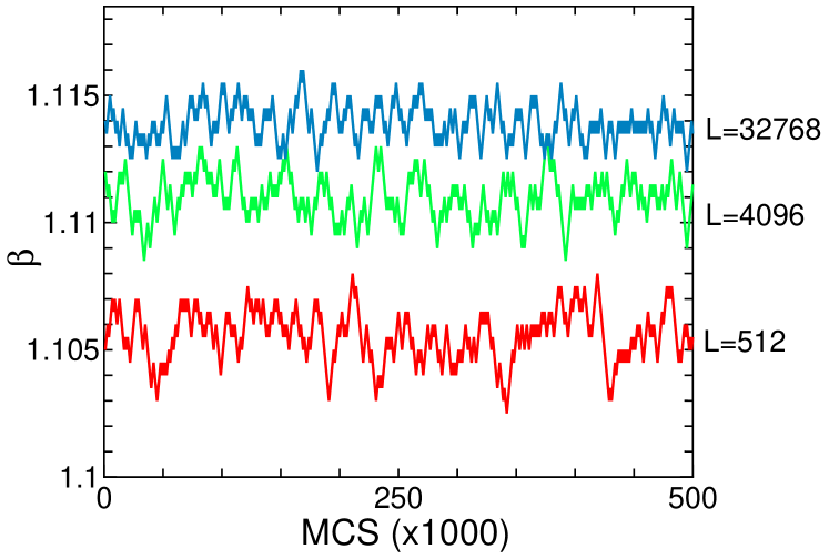
We discard 60000 Monte Carlo steps (MCS) before making a measurement. To measure the helicity modulus we take 1000 MCS. We choose $\Delta\beta$ as 0.0005. Throughout this paper we use the unit of $J=1$. First, we plot the time evolution of $\beta$ in Fig. 1. The time steps are given in units of 1000 MCS. For illustration, the data for $L$ = 512, 4096, and 32768 are shown. From Fig. 1, we see that the temperature is oscillating around the average value. The width of fluctuation becomes smaller as the system size increases because of the effect of self-averaging.

We take an average of inverse temperature over long steps; we denote it by $\beta_{\rm KT}(L)$ for each size. We tabulate $\beta_{\rm KT}(L)$ in Table 1. The numbers of measured steps in units of $10^{3}$ MCS for each size are also given in Table 1. The numbers of measured MCS range from $4\times 10^{5}$ to $4\times 10^{6}$ depending on $L$. The uncertainties of measured values, denoted in the parentheses, are estimated by the short-time average.

Table 1: Estimates of $\beta_{\rm KT}(L)$, $\langle m^{2}\rangle_{L}$ and $\xi_{\rm 2nd}(L)/L$ for the 2D classical XY model using the PCC algorithm. The numbers of measured steps in units of $10^{3}$ MCS are given.

$L$	$\beta_{\rm KT}(L)$	$\langle m^{2}\rangle_{L}$	$\xi_{\rm 2nd}(L)/L$	$10^{3}$MCS
64	1.09167(25)	0.34924(29)	0.7464(11)	4000
128	1.09788(32)	0.29695(36)	0.7466(15)	4000
256	1.10224(21)	0.25245(28)	0.7482(09)	4000
512	1.10530(26)	0.21427(27)	0.7482(14)	4000
1024	1.10768(19)	0.18195(16)	0.7488(11)	4000
2048	1.10966(20)	0.15443(26)	0.7491(14)	4000
4096	1.11097(08)	0.13085(15)	0.7495(12)	4000
8192	1.11211(27)	0.11086(32)	0.7500(21)	2000
16384	1.11314(20)	0.09395(25)	0.7492(25)	1000
32768	1.11389(21)	0.07955(22)	0.7499(22)	500
65536	1.11457(14)	0.06737(14)	0.7504(16)	400

Figure 2: (Color online) Plot of $\beta_{\rm KT}(L)$ of the 2D classical XY model for $L$ = 64, 128, 256, 512, 1024, 2048, 4096, 8192, 16536, 32768, and 65536, where $l=\ln bL$. The best fitted line, $1.11996-0.826\times l^{-2}$, is shown with $b=3.6$.

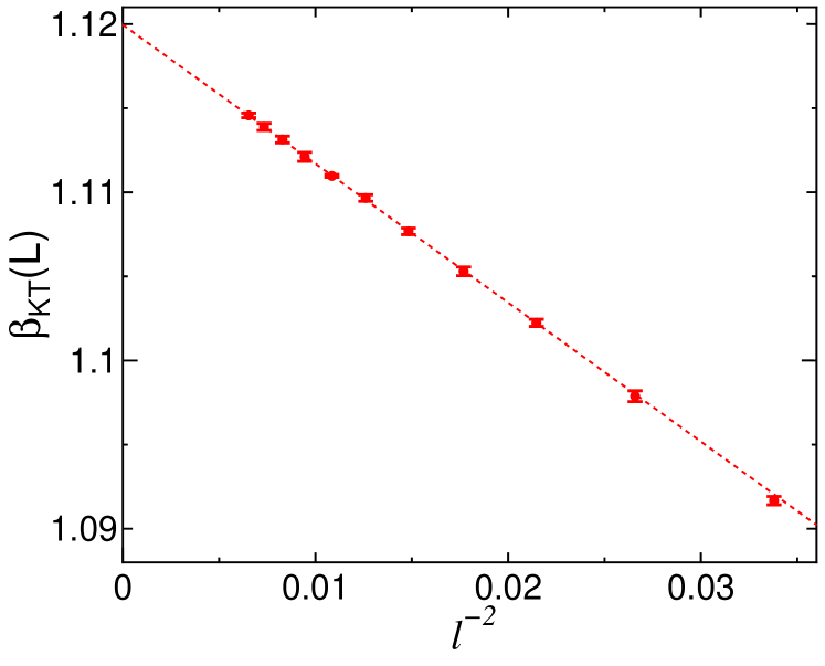
Then, we consider the size dependence of $\beta_{\rm KT}(L)$. We use the FSS analysis based on the KT form of the correlation length, Eq. (1). Using the PCC algorithm, we obtain the inverse temperature $\beta_{\rm KT}(L)$ such that the helicity modulus $\beta\Upsilon$ is $0.636508$. It means that $\xi/L(=a)$ is constant for each size. Then, using the FSS form of $\Upsilon$, that is, $\Upsilon=\Upsilon(\xi/L)$, we have the relation

$$\beta_{\rm KT}(L)=\beta_{\rm KT}-\frac{c^{2}\beta_{\rm KT}}{(\ln bL)^{2}},$$ (7)

where $b=a/A$. We plot $\beta_{\rm KT}(L)$ as a function of $l^{-2}$ with $l=\ln bL$ for the best fitted parameters in Fig. 2. The error bars, which are very small, are shown there. We try several estimates; that is, the minimum size $L$ for the check of $\chi^{2}$ values is taken as 64, 128, 256, and 512. From smaller $\chi^{2}$ values, we actually use the data of the minimum size $L$ being 128 and 256. Our estimate of $\beta_{\rm KT}$ is 1.11996(6); the numbers in the parentheses denote the uncertainty in the last digits. This value is consistent with the estimates of recent studies; 1.1199(1) by the Monte Carlo simulation [6], and 1.1200(1) by the high-temperature expansion [8].

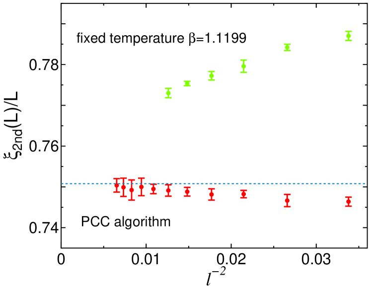
Next consider the correlation length of second moment $\xi_{\rm 2nd}(L)$;

$$\xi_{\rm 2nd}(L)=\frac{[\chi(0)/\chi(2\pi/L)-1]^{1/2}}{2\sin(\pi/L)}$$ (8)

with

$$\chi(k)=\frac{1}{N}\left|\left\langle\sum_{r}\vec{s}(r)e^{ikr}\right\rangle\right|^{2}.$$ (9)

In Ref. Hasenbusch2005, $\xi_{\rm 2nd}(L)/L$ is calculated as 0.7506912 for $L\to\infty$ at the KT temperature $T_{\rm KT}$. We tabulate $\xi_{\rm 2nd}(L)/L$ at $T_{\rm KT}(L)$ in Table 1, and plot them in Fig. 3, where the horizontal axis is chosen as the same as Fig. 2. We see that $\xi_{\rm 2nd}(L)/L$ approaches $0.750\cdots$ rapidly even for small $L$. We also make simulations at $\beta=1.1199$ to confirm the consistency with the calculation by Hasenbusch [6]. For comparison we plot $\xi_{\rm 2nd}(L)/L$ with fixing $\beta=1.1199$ in Fig. 3, which approaches $0.750\cdots$ slowly with the increase of size.

Figure 3: (Color online) Plot of $\xi_{\rm 2nd}(L)/L$ at $T_{\rm KT}(L)$ for $L$ = 64, 128, 256, 512, 1024, 2048, 4096, 8192, 16536, 32768, and 65536. The horizontal axis is the same as that of Fig. 2. The data with the PCC algorithm are compared with those at the fixed temperature $\beta=1.1199$. The calculated value for $L=\infty$ by Hasenbusch [6], $0.75069\cdots$, is given by a dotted line for convenience.

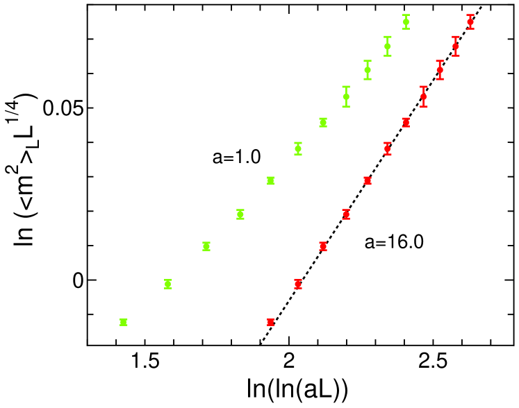
We now turn to the logarithmic-correction exponent $-2r$, given in Eq. (2). It comes from the multiplicative logarithmic corrections in terms of correlation length, such that

$$\langle m^{2}\rangle_{L}=\chi/L^{2}\propto\xi^{-\eta}(\ln\xi)^{-2r}.$$ (10)

Since we measure $\langle m^{2}\rangle_{L}$ at the temperature $T_{\rm KT}(L)$ with $\xi/L=a$ for each size, we have

$$\langle m^{2}\rangle_{L}\,L^{1/4}\propto(\ln aL)^{-2r}.$$ (11)

The measured data for $\langle m^{2}\rangle_{L}$ are tabulated in Table 1. If we take logarithm of both sides of Eq. (11), we have

$$\ln\Big{(}\langle m^{2}\rangle_{L}\,L^{1/4}\Big{)}={\rm const}-2r\ln(\ln aL).$$ (12)

We plot $\ln(\langle m^{2}\rangle_{L}L^{1/4})$ as a function of $\ln(\ln aL)$ with the best fitted parameter in Fig. 4, where $a$ is chosen as 16.0. Checking the $\chi^{2}$ values, we determine $-2r$ as 0.128(8). In Fig. 4, we also give a plot of $\ln(\langle m^{2}\rangle_{L}L^{1/4})$ as a function of $\ln(\ln L)$; that is, $a=1$. If we use only the data of $a=1$ for smaller lattices (say, $64\leq L\leq 2048$), the best fitted slope, which indicates $-2r$, in Fig. 4 becomes 0.07; whereas the slope becomes 0.11 when using only the data for larger lattices (say, $2048\leq L\leq 65536$). Thus, for large enough $L$, up to 65536, we can say that the slope, $-2r$, approaches the theoretical value 1/8 (=0.125) irrespective of the choice of $a$.

We observe that the slope, which indicates $-2r$, is smaller for small $L$ if we do not consider $a$. For large enough $L$, up to 65536, we clearly see that the slope, $-2r$, approaches the theoretical value 1/8 irrespective of the choice of $a$. We may conclude that the puzzle has been finally solved.

We note that the thermal average of the physical quantities, such as $\langle m^{2}\rangle_{L}$, with the PCC algorithm is consistent with the $T$-fix calculation within the error bars. In the PCC algorithm, $T$ is changing, but the thermal average of physical quantity coincides with the $T$-fix calculation because the fluctuation width is small enough.

We make a comment on the computational time. The GPU computation on a single NVIDIA GeForce GTX580 for the $4096\times 4096$ system takes about 14 hours, including the spin-flip and the measurement of the helicity modulus, the susceptibility, and the second-moment correlation length for 500,000 MCS. When we use multiple GPUs, the computational time for each GPU slightly increases with the increase of the number of GPUs because of the time for communication. Thus, the system of the size $65536\times 65536$ can be treated by using 256 NVIDIA Tesla M2050 GPUs in a day.

Figure 4: (Color online) Plot of $\ln(\langle m^{2}\rangle_{L}L^{1/4})$ as a function of $\ln(\ln(aL))$ at $T_{\rm KT}(L)$ for $L$ = 64, 128, 256, 512, 1024, 2048, 4096, 8192, 16536, 32768, and 65536. The best fitted line with $a=16.0$, $-0.262+0.128\times\ln(\ln(aL))$, is given. We also plot the case of $a=1.0$ for comparison

To summarize, we have studied the 2D classical XY model by a large-size cluster-update Monte Carlo simulation, and have determined $T_{\rm KT}$ using the PCC algorithm based on helicity modulus up to the size $L=65536$. The estimated inverse KT temperature is 1.11996(6). We have shown that $\xi_{\rm 2nd}(L)/L$ approaches $0.750\cdots$ rapidly with the increase of $L$ at the temperature where the helicity modulus is $0.636508\times T$. The logarithmic-correction exponent $-2r$ is estimated as 1/8 of the theoretical value with no assumption.

We have again confirmed that the self-adapted approach of the PCC algorithm is efficient to locate the critical temperature, not only for the second-order transition but also for the KT transition. We finally emphasize that GPU computation is very effective when a large-size calculation is needed, for example, for systems where logarithmic behavior is essential.