MOA-2010-BLG-311: A planetary candidate below the threshold of reliable detection

Abstract

We analyze MOA-2010-BLG-311, a high magnification ($A_{\rm max}>600$) microlensing event with complete data coverage over the peak, making it very sensitive to planetary signals. We fit this event with both a point lens and a 2-body lens model and find that the 2-body lens model is a better fit but with only $\Delta\chi^{2}\sim 80$. The preferred mass ratio between the lens star and its companion is $q=10^{-3.7\pm 0.1}$, placing the candidate companion in the planetary regime. Despite the formal significance of the planet, we show that because of systematics in the data the evidence for a planetary companion to the lens is too tenuous to claim a secure detection. When combined with analyses of other high-magnification events, this event helps empirically define the threshold for reliable planet detection in high-magnification events, which remains an open question.

1 Introduction

High-magnification events, events in which the maximum magnification of the source, $A_{\rm max}$, is greater than 100, have been a major focus of microlensing observations and analysis. Because the impact parameter between the source and the lens is very small in such cases, $u_{0}\simeq 1/A_{\rm max}$, it is likely to probe a central caustic produced by a planetary companion to the lens star. Furthermore, such events can often be predicted in advance of the peak, allowing intensive observations of the event at the time when it is most sensitive to planets. Consequently, a substantial amount of effort has been put into identifying, observing, and analyzing such events.

Observed high-magnification events are classified into two groups for further analysis: events with signals obvious to the eye and events without. Only events in the first category are systematically fit with 2(or more)-body models. The other events are only analyzed to determine their detection efficiencies. As a result, no planets have been found at or close to the detection threshold, and furthermore this detection threshold is not well understood. Gould et al. (2010) suggest a detection threshold in the range of $\Delta\chi^{2}=\,$350–700 is required to both detect the signal and constrain it to be planetary, but they note that the exact value is unknown. With the advent of second-generation microlensing surveys, which will be able to detect planets as part of a controlled experiment with a fixed observing cadence, it is important to study the reliability of signals close to the detection threshold, since a systematic analysis of all events in such a survey will yield signals of all magnitudes, some of which will be real and some of which will be spurious.

In this paper, we present the analysis of a high-magnification microlensing event, MOA-2010-BLG-311, which has a planetary signal slightly too small to claim as a detection. We summarize the data properties in Section 2 and present the color-magnitude diagram (CMD) in Section 3. In Section 4, we fit the light curve with both point lens and 2-body models. We then discuss why a planetary detection cannot be claimed in Section 4.5. We calculate the Einstein ring size and relative proper motion in Section 5 and discuss the possibility that the lens is a member of the cluster NGC 6553 in Section 6. We give our conclusions in Section 7.

2 Data

2.1 Observations

On 2010 June 15 (HJD^′ 5362.967 $\equiv$ HJD$-2450000$), the Microlensing Observations in Astrophysics (MOA) collaboration (Bond et al., 2001; Sumi et al., 2011) detected a new microlensing event MOA-2010-BLG-310 at (R.A., decl.) = (18^h08^m49.^s98, -25${}^{\circ}57^{\prime}04.\hskip-2.0pt^{\prime\prime}27$) (J2000.0), (l, b) = (5.17, -2.96), along our line of sight toward the Galactic Bulge. MOA announced the event through its email alert system and made the data available in real-time. Within a day, this event was identified as likely to reach high magnification. Because of MOA’s real-time alert system, the event was identified sufficiently far in advance to allow intensive follow up observations over the peak.

The observational data were acquired from multiple observatories, including members of the MOA, OGLE, $\mu$FUN, PLANET, RoboNet (Tsapras et al., 2009), and MiNDSTEp collaborations. In total, sixteen observatories monitored the event for more than one night, and thus their data were used in the following analysis. Among these, there is the MOA survey telescope (1.8m, MOA-Red, New Zealand) and the B&C telescope (60cm, $V$, $I$, New Zealand); eight of the observatories are from $\mu$FUN: Auckland (AO, 0.4m, Wratten #12, New Zealand), Bronberg (0.36m, unfiltered, South Africa), CTIO SMARTS (1.3m, $V$, $I$, $H$, Chile), Farm Cove (FCO, 0.36m, unfiltered, New Zealand), Kumeu (0.36m, unfiltered, New Zealand), Molehill (MAO, 0.3m, unfiltered, New Zealand), Vintage Lane (VLO, 0.4m, unfiltered, New Zealand), and Wise (0.46m, unfiltered, Israel); three are from PLANET: Kuiper telescope on Mt. Bigelow (1.55m, $I$, Arizona), Canopus (1.0m, $I$, Australia), and SAAO (1.0m, $I$, South Africa); one is from RoboNet: Liverpool (2.0m, $I$, Canaries); and one is from MiNDSTEp: La Silla (1.5m, $I$, Chile). The event also fell in the footprint of the OGLE IV survey (1.3m, $I$, Chile), which was in the commissioning phase in 2010. The observatory and filter information is summarized in Table 1.

In particular, observations from the MOA survey telescope, MOA B&C, PLANET Canopus, $\mu$FUN Bronberg, and $\mu$FUN VLO provided nearly complete coverage over the event peak between HJD${}^{\prime}=5365.0$ and HJD${}^{\prime}=5365.4$.

2.2 Data Reduction

The MOA and B&C data were reduced with the standard MOA pipeline (Bond et al., 2001). The data from the $\mu$FUN observatories were reduced using the standard DoPhot reduction (Schechter et al., 1993), with the exception of Bronberg and VLO data, which were reduced using difference image analysis (DIA; Alard, 2000; Wozniak, 2000). Data from the PLANET and RoboNet collaborations were reduced using pySIS2 pipeline (Bramich, 2008; Albrow et al., 2009). Data from MiNDSTEp were also initially reduced using the pySIS2 pipeline. The OGLE data were reduced using the standard OGLE pipeline (Udalski, 2003). Both the MOA and MiNDSTEp/La Silla data were reduced in real-time, and as such the initial reductions were sub-optimal. In fact, the original MOA data over the peak were unusable because they were corrupted. After the initial analysis, both the MiNDSTEp and MOA data were rereduced using optimized parameters.

3 Color-Magnitude Diagram

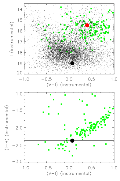
Figure 1: Color-magnitude diagram (top) and color-color diagram (bottom) of the field of view of MOA-2010-BLG-311 constructed from the CTIO observations. The small black dots represent the field stars; stars used in constructing the color-color diagram are shown as the green squares in both panels. The black line in the bottom plot shows the measured instrumental $(I-H)$ color of the source. The $(V-I)$ color of the source is then derived from the intersection of this line with the $(V-I)$—$(I-H)$ relation established by the field stars (green squares), producing the black dot in the bottom panel. The position of the source in the CMD (large black dot) is given by this $(V-I)$ measurement and the source flux from the fits to the light curve. The large red dot shows the centroid of the red clump.

To determine the intrinsic source color, we construct a color-magnitude diagram (CMD) of the field of view containing the lensing event (Figure 1) based on $V$- and $I$-band images from CTIO SMARTS ANDICAM camera. The field stars in the CMD are determined from three $V$-band images and multiple $I$-band images. Four $V$-band images were taken; however, only three of the images are of sufficient quality to contribute to the CMD. We visually checked each of the three images to make sure that there were no obvious defects such as cosmic-ray events in the images.

From the fit to the light curve, we find the instrumental magnitude of the source is $I=19.0$ with an uncertainty of 0.05 mag due to differences between the planet and point lens models as well as the error parameterizations. In the top right-hand corner of Figure 1, the red dot at $(V-I,I)_{\rm cl}=(0.40,15.5)$ marks the centroid of the red clump. The intrinsic color and magnitude of the clump are $(V-I,I)_{\rm cl,0}=(1.06,14.3)$ (Bensby et al., 2011; Nataf et al., 2012). Using the offset between the intrinsic magnitude of the clump and the observed, instrumental magnitude, we can then calibrate the magnitude of the source to find $I_{S,0}=17.8\pm 0.1$.

The color of the source is normally estimated from $V$- and $I$-band images using the standard technique in Yoo et al. (2004). However, with only one highly-magnified $V$-band image, this method is unreliable, so we use an alternative technique to determine the instrumental $(V-I)$ color by converting from the instrumental $(I-H)$ color. Using the simultaneous CTIO $I$- and $H$-band observations, we measure the instrumental $(I-H)$ color of the source by linear regression of $H$ on $I$ flux at various magnifications during the event. We then construct a $VIH$ instrumental color-color diagram from stars in the field (bottom panel of Figure 1). The stars are chosen to be all stars seen in all three bands with instrumental magnitude brighter than $H_{\rm CTIO}=19.0$ (note that the field of view for $H$-band observations is $2.4^{\prime}\times 2.4^{\prime}$ compared to $6^{\prime}\times 6^{\prime}$ for the optical bands). The field stars form a well defined track, which enables us to estimate the $(V-I)$ source color from the observed $(I-H)$ source color. This yields $(V-I)_{0}=0.75\pm 0.05$. Note that this method would not work for red stars, $(V-I)_{0}>1.3$, because for these red stars, the $VIH$ relation differs between giants and dwarfs (Bessell & Brett, 1988). However, the observed color is well blueward of this bifurcation. There is also a spectrum of the source taken at HJD${}^{\prime}=5365.001$ (Bensby et al., 2011). The “spectroscopic” $(V-I)_{0}$ reported in that work is 0.77, in good agreement with the value calculated here.

4 Modeling

4.1 The Basic Model

A casual inspection of the light curve does not show any deviations from a point lens, so we begin by fitting a point lens model to the data. A point lens model is characterized by three basic parameters: the time of the peak, $t_{0}$, the impact parameter between the source and the lens stars, $u_{0}$, and the Einstein timescale, $t_{E}$. Since $u_{0}$ is small, the finite size of the source can be important. To include this effect, we introduce the source size in Einstein radii, $\rho$, as a parameter in the model. Additionally, we include limb-darkening of the source. The temperature of this slightly evolved source was determined from the spectrum to be $T_{\rm eff}\sim$ 5460 K by Bensby et al. (2011). Using Claret (2000) we found the limb-darkening coefficients to be $u_{V}=0.7086$, $u_{I}=0.5470$, and $u_{H}=0.3624$, assuming a microturbulent velocity = 1 km s^-1, log $g$ = 4.0, solar metallicity, and $T_{\rm eff}=5500$K, which is the closest grid point given the Bensby et al. (2011) measurements. We then convert $u_{V}$, $u_{I}$, and $u_{H}$ to the form introduced by Albrow et al. (1999)

$$\Gamma=\frac{2u}{3-u}$$ (1)

to obtain $\Gamma_{V}=0.62$, $\Gamma_{I}=0.45$, and $\Gamma_{H}=0.28$. Because the various data sets are not on a common flux scale, there are also two flux parameters for each data set, $f_{\rm S,i}$ and $f_{\rm B,i}$, such that

$$f_{{\rm mod},i}=f_{{\rm S},i}A(t)+f_{{\rm B},i},$$ (2)

where $A(t)$ is the predicted magnification of the model at time, $t$, and includes the appropriate limb-darkening for data set $i$. The source flux is given by $f_{{\rm S},i}$, and $f_{{\rm B},i}$ is the flux of all other stars, including any light from the lens, blended into the PSF (i.e., the “blend”).

4.2 Error Renormalization

As is frequently the case for microlensing data, the initial point lens fit reveals that the errors calculated for each data point by the photometry packages underestimate the true errors. Additionally, there are be outliers in the data that are clearly seen to be spurious by comparison to other data taken simultaneously from a different site. Simply taking the error bars at face value would lead to biases in the modeling. Because the level of systematics varies between different data sets, underestimated error bars can give undue weight to a particular set of data. Additionally, if the errors are underestimated, the relative $\Delta\chi^{2}$ between two models will be overestimated, making the constraints seem stronger than they actually are.

To resolve these issues, we rescale the error bars using an error renormalization factor (or factors) and eliminate outliers. We begin by fitting the data to a point lens to find the error renormalization factors. We remove the outliers according to the procedure described below based on the renormalized errors, refit, and recalculate the error renormalization factors. We repeat this process until no further outliers are found.

To first order, we can compensate for the underestimated error bars by rescaling them by a single factor, $k$. The rescaling factor is chosen for each data set, $i$, such that $k_{i}=(\chi_{i}^{2}/N_{i})^{1/2}$, producing a $\chi^{2}$ per degree of freedom of $\chi^{2}_{\rm dof}=1$. We will refer to this simple scheme for renormalizing the errors as “1-parameter errors”.

Alternatively, we can use a more complex method to renormalize the errors, which we will call “2-parameter errors”. This method was also used in Miyake et al. (2012) and Bachelet et al. (2012a). To renormalize the errors, we rank order the data by magnification and calculate two factors, $k$ and $e_{\rm min}$, such that

$$\sigma_{j}=k_{i}\sqrt{\sigma_{{\rm orig},j}^{2}+e_{{\rm min},i}^{2}},$$ (3)

where $\sigma_{\rm orig}$ is the original error bar and $\sigma$ is the new error bar and the calculations are done in magnitudes. The index $i$ refers to a particular data set, and $j$ refers to a particular point within that data set. The additional term, $e_{\rm min}$, enforces a minimum uncertainty in magnitudes, because at high magnification, the flux is large, so the formal errors on the measurement can be unrealistically small. The error factors, $k$ and $e_{\rm min}$, are chosen so that $\chi^{2}_{\rm dof}$ for points sorted by magnification increases in a uniform, linear fashion and $\chi^{2}_{\rm dof}=1$ (Yee et al., 2012). Not all data sets will require an $e_{\rm min}$ term; it is only necessary in cases for which $\chi^{2}_{\rm dof}$ has a break because the formal errors are too small when the event is bright. Note that the $e_{\rm min}$ factor will be primarily affected by the points taken when the event is bright, whereas $k$ is affected by all points, so if there are many more points at the baseline of the event, these will dominate the calculation of $k$.

To remove outliers in the data we begin by eliminating any points taken at airmass $>3$ or during twilight. Additional outliers are defined as any point more than $X\sigma$ from the expected value, where $X$ is determined by the number of data points, such that fewer than one point is expected to be more than $X\sigma$ from the expected value assuming a Gaussian error distribution. The normal procedure is to compare the data to the “expected value” from a point lens fit. We do this for data in the wings of the event, $t($HJD${}^{\prime})<5363$ or $t($HJD${}^{\prime})>5367$, when we do not expect to see any real signals. However, the peak of the event, $5365\leq t($HJD${}^{\prime})\leq 5367$, is when we would expect to see a signal from a planet if one exists. A planetary signal would necessarily deviate from the expectation for a point lens, so in this region instead of comparing to a point lens model, we use the following procedure to identify outliers:

1. For each point, we determine whether there are points from any other data set within 0.01 days. If there are more than two points from a given comparison dataset in this range, we keep only the point(s) immediately before and/or after the time of the point in question (i.e., a maximum of 2 points). The point is not compared to other points from the same data set.

2. If there are matches to at least two other data sets, we proceed to (4) to determine whether or not the point is an outlier. Otherwise, we treat the point as good.

3. We then determine the mean of the collected points, $\mu$, including the point in question, by maximizing a likelihood function for data with outliers (Sivia & Skilling, 2010):

   $$L\propto\sum_{j=1}^{N}\ln\left(\frac{1-e^{-R_{j}^{2}/2}}{R_{j}^{2}}\right)$$ (4)

   where $R_{j}=(\mu-x_{j})/\sigma_{j}$ and $x_{j}$ is the datum and $\sigma_{j}$ is its renormalized error bar. If the flux is changing too rapidly for the points to be described well by a mean, we fit a line to the data.

4. We compare the point to the predicted value, using the likelihood function to see if it is an outlier:

   (a) If there is only one likelihood maximum, we calculate $R_{j}$. If $R_{j}>X$, the point is rejected as an outlier.

   (b) If there is more than one maximum, and the point in question falls in the range spanned by the maxima, we assume the point is good. If it falls outside the range, we calculate $R_{j}$ using the nearest maximum to determine $\mu$. If $R_{j}>X$, we flag the point as an outlier.

Note that for this procedure, we use the point lens model values of $F_{\rm S,i}$ and $F_{\rm B,i}$ to place all of the data sets on a common flux scale.

This procedure is more complicated than usual, but because we compare the points only to other data, rather than some unknown model, it provides an objective means to determine whether a point is an outlier without destroying real signals corroborated by other data. We also visually inspect each set of points to confirm that the algorithm works as expected. Because finite source effects are significant in this event, one might expect slight differences among data sets due to the different filters, so as part of this visual inspection we also checked that this did not play a significant role.

For both 1-parameter and 2-parameter errors, Table 1 lists the error normalization factors and number of points for each observatory that survived the rejection process. Which of these error parameterizations correctly describes the data depends on the nature of the underlying errors. In principle, the noise properties of the data are fully described by a covariance matrix of all data points, but we are unable to calculate such a matrix. Instead, we have two different error parameterizations. The $k$ factor is calculated primarily based on baseline data for which statistical errors dominate. In contrast, the $e_{\rm min}$ factor is heavily influenced by points at the peak of the event when systematic errors are important. Thus, 2-parameter errors better reflect the systematic errors, whereas 1-parameter errors better reflect the statistical errors.

Correlated errors often have a major impact on our ability to determine whether or not the planetary signal in this event is real. We know that correlations in the microlensing data exist, but there has not been a systematic investigation of this in the microlensing literature. Correlated errors (red noise) are generally thought of as reducing the sensitivity to signals, because successive points are not independent, giving related information. But in fact, sharp, short timescale signals are not degraded by correlated noise and may still be robustly detected.

Consider the case of a short-timescale signal superimposed on a long-timescale correlation. Then a model may reproduce the short-timescale signal leading to an improvement in $\chi^{2}$ without actually passing through the data because of the overall offset caused by the correlations. Now suppose that the correlated, red noise has a larger-amplitude than the white noise (i.e., statistically uncorrelated noise). If we set the error bars by the large-amplitude deviations, which is correct for long timescales for which the data are uncorrelated, the significance of the short timescale jump will be diluted, possibly to the point of being considered statistically insignificant. However, if the timescale of the signal is much shorter than the correlation length of the red noise, the significance of the signal should actually be judged against the white noise, since on that timescale, the red noise will only contribute a constant offset.

In this case, we expect the planetary signal to be quite short, so if the systematic noise is dominated by correlated errors, the noise should be better described by the 1-parameter errors. Because the source in this event crosses the position of the lens and there are no obvious deviations due to a planet, we expect that any planetary signals will be due to very small caustics, which are detectable only at the limb-crossing times ($t_{\rm limb}=t_{0}\pm t_{E}\sqrt{\rho^{2}-u_{0}^{2}}$) when the caustic passes onto and off-of the face of the source. Therefore, the timescale of such a perturbation will be very short, equal to $t_{\rm E}$ times the caustic size $w$, which is $\lesssim 15$ minutes. In contrast, observed correlations in the microlensing data are typically on longer timescales, $\mathcal{O}($hour$)$ (based on our experience with microlensing data which are usually sampled with a frequency of $\sim 15$ minutes). Hence, the timescale of the signal is likely to be less than the timescale of the correlated noise.

However, there are other sources of systematic errors that are unrelated to correlated noise such as flat-fielding errors. If such errors dominate over correlated noise, then the 2-parameter errors are a better description of the error bars over the peak.

Because the systematic errors, correlated and uncorrelated, have not been studied in detail, we are unable to determine which is the dominant effect. Hence, we are also unable to determine which error prescription better describes our data. We will begin by analyzing the light curve using 1-parameter errors. We will then discuss how the situation changes for 2-parameter errors.

4.3 Point Lens Models

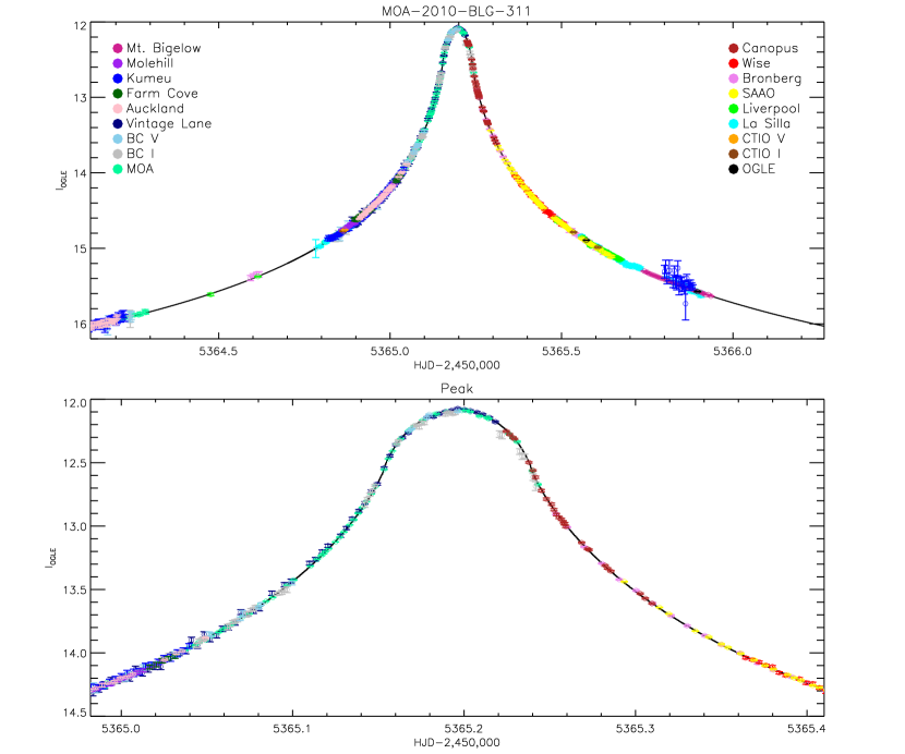
Figure 2: Light curve of MOA-2010-BLG-311. Data from different observatories are plotted in different colors. The data from Bronberg (medium pink) have been binned for clarity in the figures; only unbinned data were used in the fitting. The black line shows the best-fit point lens model; on this scale, the best-fit planetary model appears very similar. The error bars reflect 1-parameter errors (see Sec. 4.2).

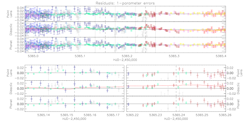
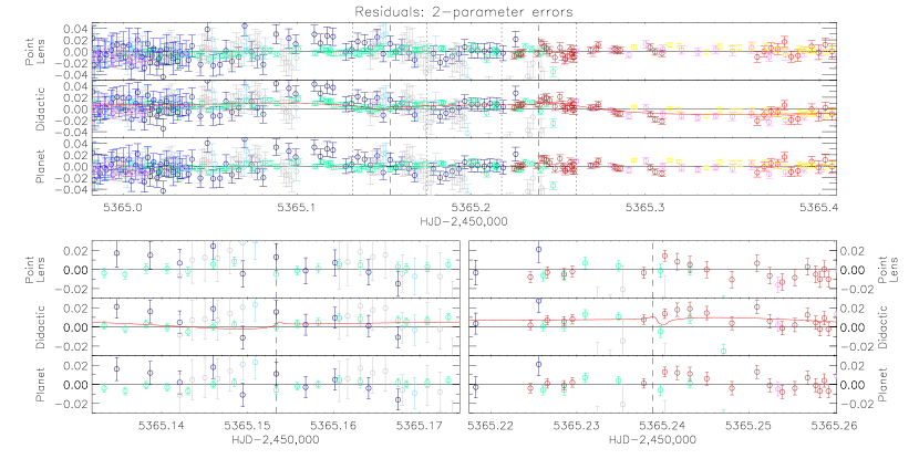
Figure 3: Residuals over the peak to the best-fit point lens and planetary microlensing models. The top set of panels shows 1-parameter errors, and the bottom set shows 2-parameter errors. Note that for the time range shown, which is the same as for the bottom panel for Fig. 2, the error bars tend to be larger for 2-parameter errors than for 1-parameter errors. Careful inspection of the residuals to the point lens and planet models shows improvement around the times of the limb-crossings of the source star and also on the falling side of the light curve. In the middle panel of each set, the red lines show the difference between the best planetary and best point lens models. The didactic residuals in the middle panel are the sum of the red line and the residuals to the best planet model (bottom panel). The dashed lines indicate the limb-crossing times. The dotted lines in the top panels of each set indicate the time ranges shown in the bottom panels. Note that the scales for the top and bottom residuals panels are not the same. The colors of the points are the same as in Fig. 2. The Bronberg data have been binned for clarity (as in Fig. 2)

The best-fit point lens model and the uncertainties in the parameters are given in Table 2. This model is shown in Figure 2, and the residuals to this fit are shown in Figure 3. These exhibit no obvious deviations. These fits confirm that finite source effects are important, since $\rho$ is well measured and larger than the impact parameter, $u_{0}$.

We also fit a point lens model that includes the microlens parallax effect, which arises either from the orbital motion of the Earth during the event or from the difference in sightlines from two or more observatories separated on the surface of the Earth. Microlens parallax enters as a vector quantity: ${\mbox{\boldmath$\pi$}}_{\rm E}=(\pi_{\rm E,N},\pi_{\rm E,E})$. The addition of parallax can break the degeneracy between solutions with $u_{0}>0$ and $u_{0}<0$, so we fit both cases. Parallax does improve the fit beyond what is expected simply from adding 2 more free parameters and shows a preference for $u_{0}>0$. However, we shall see in the next section that a planetary model without parallax produces an even better fit and adding parallax in addition to the planet gives only a small additional improvement.

4.4 2-body Models

We search for 2-body models over a broad range of mass ratios, from $q=10^{-6}$ to $q=10^{-1}$. For each value of $q$, we chose a range for the projected separation between the two bodies, $s$, for which the resulting caustic is smaller than $\rho$ and $s<1.0$. For each combination of $s$ and $q$, we allow the angle of the source trajectory, $\alpha$, to vary, seeding each run with values of $\alpha$ from 0 to 360 degrees in steps of 5 degrees. For our models, we use the map-making method of Dong et al. (2006) when the source is within two source radii of the position of the center of magnification. Outside this time range, we use the hexadecapole or quadrupole approximations for the magnification (Pejcha & Heyrovský, 2009; Gould, 2008). We used a Markov Chain Monte Carlo to find the best-fit parameters and uncertainties for each $s$, $q$ combination.

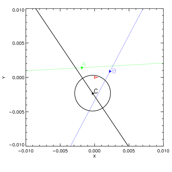
Figure 4: The caustic (red) and three source trajectories corresponding to the three minima discussed in Section 4.4. Trajectory C (black) is preferred by $\Delta\chi^{2}\gtrsim 35$ over trajectories A (green) and B (blue) for models with 1-parameter errors and without parallax. The source is shown to scale as the large circle; the lines with arrows indicate the trajectories of the center of the source. The abscissa in these plots is parallel to the binary axis with the lens star close to the origin and planet to the right. The scale is such that 1.0 equals the Einstein radius.

The grid search reveals an overall improvement in $\chi^{2}$ relative to the point lens model. We find three $\chi^{2}$ minima for different angles for the source trajectory. For central caustics with planetary mass ratios, the caustic is roughly triangular in shape with a fourth cusp where the short side of the triangle intersects the binary axis; the three trajectories roughly correspond to the three major cusps of the caustic. An example caustic is shown in Figure 4 along with the trajectories corresponding to the three minima. The angles of the three trajectories are approximately $\alpha=0,115,$ and 235 degrees, and we will refer to them as trajectories “A”, “B”, and “C”, respectively.

We then refine our grid of $s$ and $q$ around each of these three minima. We repeat these fits accounting for various microlensing degeneracies. First, we fit without parallax and assuming $s<1$. Then, we add parallax and fit both with $u_{0}>0$ and $u_{0}<0$ to see if this degeneracy is broken. Finally, we fit 2-body lens models with $s>1$ and no parallax, since there is a well known microlensing degeneracy that takes $s\rightarrow s^{-1}$.

The best-fit solution has $\chi^{2}=6637.96$ and $\alpha=236.4$. This reflects an improvement in $\chi^{2}$ of $\Delta\chi^{2}\sim 140$ over the point lens solution. There is no preference for $s<1$ over $s>1$, but trajectory C is preferred by $\Delta\chi^{2}\gtrsim 35$ over trajectories A and B. The parameters and their uncertainties for the planet fits are given in Table 2. The mass ratio between the lens star and its companion is firmly in the planetary regime: $q=10^{-3.7\pm 0.1}$. Furthermore, planetary mass ratios are clearly preferred over “stellar” mass ratios ($q\sim 0.1$), which are disfavored by more than $\Delta\chi^{2}=60$. Parallax further improves the fit by only $\Delta\chi^{2}\sim 10$ and has little effect on the other parameters.

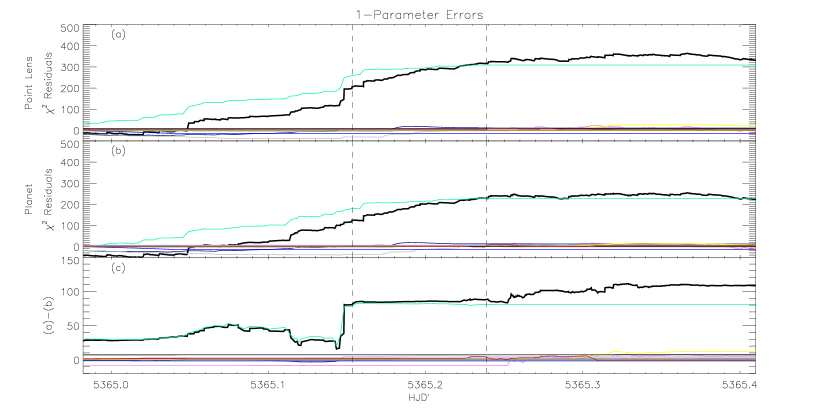
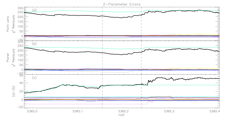
Figure 5: The difference between the cumulative $\chi^{2}$ distribution and the expected distribution ($\sum_{j}^{N}\chi^{2}_{j}=N$), i.e. the $\chi^{2}$ residuals, for both 1-parameter (top) and 2-parameter (bottom) errors. The top two panels of each set show the distributions for the point lens model (a) and the planetary models (b). The bottom panels (c) of each set show the difference between the top and middle panels. The distributions for each data set are plotted separately and are shown over the same time range as the bottom panel of Fig. 2; data sets without points in this time range are not shown. The colors are as in Fig. 2. The thick black line shows the total distribution for all data. The limb-crossing times are indicated by the dashed lines. Note the jump in the MOA data (light green) at the time of the first limb-crossing (HJD${}^{\prime}\sim 5361.5$). The signal is much more pronounced for 1-parameter errors than for 2-parameter errors. Note that the vertical scales in the two sets of panels are different.

To compare the point lens and planetary models, in Figure 5, we plot the “$\chi^{2}$ residuals”: the difference between the cumulative $\chi^{2}$ distribution and the expected value $\sum_{j}^{N}\chi^{2}_{j}=N$, i.e. each point is expected to contribute $\chi^{2}_{j}=1$. For both the point lens and the planet fits, the distribution rises gradually over the peak of the event. This is expected since 1-parameter errors do not account for correlated noise. However, in the $\chi^{2}$ residuals for the point lens, there is a jump seen at the time of the first limb-crossing. This jump is even more pronounced when looking at the difference between the planet and point lens models. The jump is caused by MOA data at the time of the limb-crossing that do not fit the point lens well, thereby causing an excess increase in $\chi^{2}$. This is exactly the time when we expect to see planetary signals.

Finally, given the extreme finite source effects in this event, we might be concerned that uncertainties in the limb-darkening coefficients due to uncertainties in the source properties could influence our conclusions. The planetary signal has two components: a limb-crossing signal and an asymmetry. The limb-darkening could influence the first signal, but not the second. To check that the limb-darkening coefficients do not significantly influence our results, we repeat the point lens fits allowing the limb-darkening coefficients to be free parameters. In all cases (no parallax, parallax, 1-parameter or 2-parameter errors), the improvement to the fit from free limb-darkeing is $\Delta\chi^{2}\lesssim 10$, much smaller than the planetary signal. Furthermore, the value of $\Gamma_{V}$ decreases by $>10\%$, which is excluded by the measured source parameters. Thus, we conclude that our treatment of the limb-darkening is reasonable.

4.5 Reliability of the Planetary Signal

Although $\Delta\chi^{2}\sim 140$ appears to be significant, we are hesitant to claim a detection of a planet. The planetary signal is more or less equally divided between the jump at the first limb-crossing and a more gradual rise after the second limb-crossing (see the third panel of Fig. 5 showing the difference between the point lens and planet models). One could argue that the gradual rise, due to a slight asymmetry in the planet light curve, could be influenced by large-scale correlations in the data. Comparing Figures 3 and 5 shows that most of the signal at the first limb-crossing comes from only a few points. A careful examination of the residuals in Figure 3 shows that while the residuals to the planet model are smaller than for the point lens model, they are not zero, and the didactic residuals do not go neatly through the difference between the models as they do for MOA-2008-BLG-310 (Janczak et al., 2010). Hence, the evidence for the planet is not compelling.

If we repeat the analysis using 2-parameter errors, we find a similar planetary solution, although the exact values of the parameters are slightly different. The total signal from the planet is significantly degraded for 2-parameter errors, with only $\Delta\chi^{2}\sim 80$ between the best-fit planet and point lens models. Table 3 gives parameters for the complete set of point lens and planet fits for 2-parameter errors. The residuals and error bars over peak may be compared to 1-parameter errors in Figure 3.

We also show the $\chi^{2}$ residuals for 2-parameter errors in the bottom set of panels in Figure 5. They are more or less flat over the peak, showing that they track the data well in this region. The offset from zero is caused by systematics elsewhere in the light curve. The difference plot (bottom-most panel) shows that the planet fit is still an improvement over the point lens fit, but the signal from the planet at the first limb-crossing is much weaker. This is a natural consequence of 2-parameter errors, since the data at the peak of the event, where the planetary signal is seen, have much larger renormalized error bars than for 1-parameter errors.

Regardless of the error renormalization, this planetary signal is smaller than the $\Delta\chi^{2}$ of any securely detected high-magnification microlensing planet. Previously, the smallest $\Delta\chi^{2}$ ever reported for a high-magnification event was for MOA-2008-BLG-310 with $\Delta\chi^{2}=880$ (Janczak et al., 2010). Yee et al. (2012) discuss MOA-2011-BLG-293, an event for which the authors argue the planet could have been detected from survey data alone with $\Delta\chi^{2}=500$. However, although the planet is clearly detectable at this level, it is unclear with what confidence the authors would have claimed the detection of the planet in the absence of the additional followup data, which increases the significance of the detection to $\Delta\chi^{2}=5400$. At an even lower level, Rhie et al. (2000) find that a planetary companion to the lens improves the fit to MACHO-98-BLG-35 at $\Delta\chi^{2}=20$, but they do not claim a detection. As previously mentioned, Gould et al. (2010) suggest the minimum “detectable” planet will have $350<\Delta\chi^{2}<700$. However, this threshold has not been rigorously investigated; the minimum $\Delta\chi^{2}$ could be smaller.

Because of the tenuous nature of the planetary signal, we do not claim to detect a planet in this event, but since including a planet in the fits significantly improves the $\chi^{2}$, we will refer to this as a “candidate” planet.

Finally, it is interesting to note that even though the $\Delta\chi^{2}$ for the planetary model is too small to be considered detectable, for both 1-parameter and 2-parameter errors the parameters of the planet ($s$ and $q$) are well defined (see Tables 2 and 3). Central caustics can be degenerate, especially when they are much smaller than the source size, so we might expect a wide range of possible mass ratios in this case since the limb-crossings are not well-resolved (Han, 2009). However, perhaps we should not be surprised that the planet parameters are well-constrained: both $\Delta\chi^{2}=80$ and $\Delta\chi^{2}=140$ are formally highly significant, which would plausibly lead to reasonable constraints on the parameters. In this case, because we believe that the signal could be caused by systematics, by the same token, the constraints on the parameters may be over-strong. We conjecture that the limb-crossing signal does not constrain $q$ and that this constraint actually comes from the asymmetry of the light curve, since small, central caustics due to planets are asymmetric whereas those due to binaries are not.

5 $\theta_{\rm E}$ and $\mu_{\rm rel}$

Because the source size, $\rho$, is well measured, we can determine the size of the Einstein ring, $\theta_{\rm E}$, and the relative proper motion between the source and the lens, $\mu_{\rm rel}$ from the following relations:

$$\theta_{{\rm E}}=\frac{\theta_{\star}}{\rho} \mathrm{and} \mu_{\rm rel}=\frac{\theta_{{\rm E}}}{t_{{\rm E}}}.$$ (5)

Keeping the limb-darkening parameters fixed, we find the best fit for the normalized source size to be $\rho=(2.70\pm 0.06)\times 10^{-3}$ for the planetary fits; the value is comparable for the point lens fits. We convert the $(V-I)$ color to $(V-K)$ using Bessell & Brett (1988) and obtain the surface brightness by adopting the relation derived by Kervella et al. (2004). Combining the dereddened $I$ magnitude with this surface brightness yields the angular source size $\theta_{\star}=1.03\pm 0.07\ \mu{\rm as}$. The error on $\theta_{\star}$ combines the uncertainties from three sources: the uncertainty in flux ($f_{s,I}$), the uncertainty from converting $(V-I)$ color to the surface brightness, and the uncertainty from the Nataf et al. (2012) estimate of $I_{\rm 0,cl}$. The uncertainty of $f_{s,I}$ is 3%, which is obtained directly from the modeling output. We estimate the uncertainty from the other factors ($Z$) to be 7%. The fractional error in $\theta_{\star}$ is given by $[(1/4)(\sigma_{f_{s,I}})^{2}+(\sigma_{Z}/Z)^{2}]^{1/2}$ = 7%, which is also the fractional error of the proper motion $\mu$ and the Einstein ring radius $\theta_{{\rm E}}$ (Yee et al., 2009). Thus, we find $\theta_{\rm E}=0.38\pm 0.03$ mas and $\mu_{\rm rel}=7.1\pm 0.6$ mas yr^-1.

6 The Lens as a Possible Member of NGC 6553

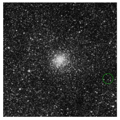
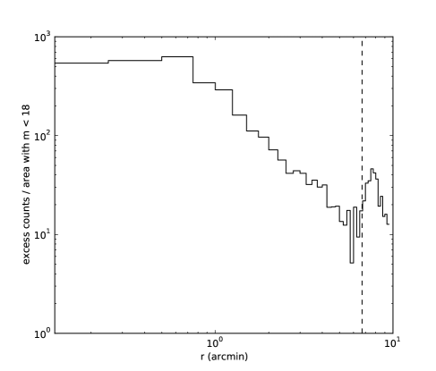
Figure 6: DSS image of NGC 6553 (left). The position of the microlensing event is indicated by the circle. Excess star density over the background around the globular cluster NGC 6553 (right). The center of the cluster is placed at $r=0$. The microlensing event is at $r=6.7^{\prime}$ (dashed line). The dip at $\sim 6^{\prime}$ is caused by a quasi-circular dust lane, which may be seen in the image. Even though the density of stars drops quickly as a function of radius, cluster members still comprise about 6% of the stars at $r=6.7^{\prime}$.

This microlensing system is close in projection to the globular cluster NGC 6553. The cluster is at (R.A., decl.) = (18^h09^m17.^s60, -25${}^{\circ}54^{\prime}31.\hskip-2.0pt^{\prime\prime}3$) (J2000.0), with a distance of 6.0 kpc from the Sun and 2.2 kpc from the Galactic Center (Harris, 1996). The half-light radius $r_{h}$ of NGC 6553 is $1.03^{\prime}$ (Harris, 1996), which puts the microlensing event 6.5 half-light radii ($6.7^{\prime}$) away from the cluster center. By plotting the density of excess stars over the background, we find that about 6% of the stars at this distance are in the cluster (Figure 6).

Whether or not the lens star is a member of the cluster can be constrained by calculating the proper motion of the lens star. Zoccali et al. (2001) found a relative proper motion of NGC 6553 with respect to the Bulge of ${\mbox{\boldmath$\mu$}}=(\mu_{l},\mu_{b})=(5.89,0.42)$ mas yr^-1. The typical motion of Bulge stars is about $100\,\rm km\,s^{-1}$ corresponding to about $3\,\rm mas\,yr^{-1}$ given an estimated distance of 7.7 kpc toward the source along this line of sight ($l=5.1^{\circ}$; Nataf et al., 2012). Therefore the expected amplitude of the lens-source relative proper motion if the lens is a cluster member is $\mu_{\rm rel}=7\pm 3\,\rm mas\,yr^{-1}$, which is consistent with the measured value in Section (5).

Combining the measurement of the stellar density with the proper motion information, we find the probability that the lens is a cluster member is considerably higher than the nominal value based only on stellar density. First, of order half the stars in the field are behind the source, whereas the lens must be in front of the source. Second, the lens-source relative proper motion is consistent with what would be expected for a cluster lens at much better than $1\,\sigma$, which is true for only about 2/3 of events seen toward the Bulge. Combining these two effects, we estimate a roughly 18% probability that the lens is a cluster member.

One way to resolve this membership issue is by measuring the true proper motion of the lens as was done for a microlensing event in M22 for which the lens was confirmed to be a member of the globular cluster (Pietrukowicz et al., 2012). For this event, we have calculated the relative proper motion of the lens and the source to be $7.1\pm 0.6{\rm\ mas\ yr}^{-1}$. This is consistent with the expected value if the lens were a member of the cluster. About 10 years after the event, the separation between the lens and the source star will be large enough to be measured with $HST$. Based on this followup observation, one will be able to clarify whether the lens is a member of the cluster by measuring the vector proper motion. If it is a member of the cluster, its mass may be estimated from

$$M_{\rm lens}=\frac{\theta_{\rm E}^{2}}{\kappa\pi_{{\rm rel}}},$$ (6)

where $\kappa\equiv 4G/c^{2}{\rm AU}=8.14\ {\rm mas}/M_{\sun}$ and $\pi_{{\rm rel}}$ is the source-lens relative parallax. In addition, the metallicity of the lens could be inferred from the metallicity of the globular cluster.

7 Discussion

We have found a candidate planet signal in MOA-2010-BLG-311. The evidence in support of the planet is

1. The planet substantially improves the fit to the data,

2. In addition to a general improvement to the light curve, the planet produces a signal when we most expect it, i.e. the time of the first limb-crossing,

3. The solution has a well-defined mass ratio and projected separation for the planet (excepting the well known $s\rightarrow s^{-1}$ degeneracy).

The magnitude of the signal depends on whether the error bars are renormalized using 1-parameter ($\Delta\chi^{2}=140$) or 2-parameter error factors ($\Delta\chi^{2}=80$). We conservatively adopt $\Delta\chi^{2}=80$ as the magnitude of the signal, but note that if correlated errors are the dominant source of systematic uncertainty, $\Delta\chi^{2}=140$ should be adopted instead (see Section 4.2). Regardless, this signal is too small to claim as a secure detection.

Examining the residuals to the light curve and the $\chi^{2}$ residuals shows that the planetary signal is dispersed over many points at the peak of the light curve. It comes from an overall asymmetry near the peak plus a few points at the limb-crossing. Because the signal is the sum of multiple cases of low-amplitude deviations, it is plausible that the microlensing model could be fitting systematics in the data, which is why the planet signal is not reliable.

Combined with other studies, this event suggests that central-caustic (high-magnification) events and planetary-caustic events require different detection thresholds. The detection threshold suggested in Gould et al. (2010) of $350<\Delta\chi^{2}<700$ was made in the context of high-magnification events, and our experience so far is consistent with this. A planet was clearly detectable in MOA-2008-BLG-310 with $\Delta\chi^{2}=880$ (Janczak et al., 2010). However, Yee et al. (2012) are uncertain if a planet would be claimed with $\Delta\chi^{2}=500$ for MOA-2011-BLG-293. Here, $\Delta\chi^{2}=80$ is definitely insufficient to detect a planet. Hence, the detection threshold for planets in high-magnification events is around or just below $\Delta\chi^{2}=500$. In contrast, the planetary caustic crossing in OGLE-2005-BLG-390 produced a clear signal of $\Delta\chi^{2}=532$ (Beaulieu et al., 2006), and the planet would most likely be detectable if the error bars were 50% larger ($\Delta\chi^{2}\sim 200$) and might even be considered reliable if the error bars were twice as large.

We suspect the reason for the different detection thresholds is that the information about the microlens parameters and the planetary parameters comes from different parts of the light curve. For planetary-caustic events, the planet signal is a perturbation separated from the main peak. Thus, the microlens parameters can be determined from the peak data independently from the planetary parameters, which are measured from the separate, planetary perturbation. In contrast, for high-magnification events, the planetary perturbation occurs at the peak of the event, so the microlens and planetary parameters must be determined from the same data.

The detection threshold for planetary-caustic events will have to be investigated in more detail. If it is truly lower than for high-magnification events, this is good news for second generation microlensing surveys since that is how most planets will be found in such surveys. At the same time, it points to the continued need for followup data of high-magnification events since these seem to have a higher threshold for detection, requiring more data to confidently claim a planet. This is an important consideration because high-magnification events can yield much more detailed information about the planets.

Additionally, Han & Kim (2009) show that the magnitude of the planetary signal should decrease as the ratio between the caustic size and the source size ($w/\rho$) decreases for the same photometric precision. There are several cases of events for which $w/\rho\lesssim 1$: in this case, we have $w/\rho=0.12$ and $\Delta\chi^{2}=140$; the brown dwarf in MOA-2009-BLG-411L has $w/\rho=0.3$ and $\Delta\chi^{2}=580$ (Bachelet et al., 2012b); MOA-2007-BLG-400 has $w/\rho=0.4$ and $\Delta\chi^{2}=1070$ (Dong et al., 2009); and in the case of MOA-2008-BLG-310, the value is $w/\rho=1.1$ with $\Delta\chi^{2}=880$ (Janczak et al., 2010). This sequence is imperfect, but the photometry in the four cases is far from uniform, and it seems that in general the trend suggested by Han & Kim (2009) holds in practice.

Finally, we note that a large fraction of the planet signal comes from the MOA data, but in the original, real-time MOA data, this signal would not have been detectable since the data were corrupted over the peak of the event. It is only after the data quality was improved by rereductions, which in turn were undertaken only because the event became the subject of a paper, that we recovered the planet candidate. This points to the importance of rereductions of the data when searching for small signals. In the current system of analyzing only the events with the most obvious signals, this is not much of a concern. However, if current or future microlensing surveys are systematically analyzed to find signals of all sizes, this will become important.

Acknowledgments

.

Table 1: Data Properties for Two Methods of Error Renormalization. The observatories are listed in order of longitude starting with the most Eastward. If data were taken in more than one filter at a given site, different filters are given on successive lines. The error renormalization coefficients and method for removing outliers are described in Section 4.2.

		1-parameter Errors		2-parameter Errors
Observatory	Filter	$k$	$N_{\rm data}$	$k$	$e_{\rm min}$	$N_{\rm data}$
Mt. Bigelow	I	1.63	44	1.63	0.0	44
Molehill	Unfiltered	0.72	69	0.72	0.0	69
Kumeu	Wratten #12	1.19	188	1.18	0.0	188
Farm Cove	Unfiltered	1.27	52	1.26	0.0	52
Auckland	Wratten #12	0.98	84	1.00	0.0	84
Vintage Lane	Unfiltered	4.87	112	3.05	0.004	112
B&C	I	4.07	132	1.01	0.025	136
	V	1.15	53	0.66	0.03	55
MOA	MOA-Red	1.68	4452	1.55	0.003	4434
Canopus	I	3.02	28	2.87	0.0	29
Wise	Unfiltered	0.52	70	0.53	0.0	70
Bronberg	Unfiltered	1.26	727	1.27	0.0	727
SAAO	I	2.60	128	2.21	0.0015	127
Liverpool	SDSS-i	1.85	120	1.04	0.007	119
La Silla	I	10.02	169	3.79	0.004	174
CTIO	I	1.33	22	1.34	0.0	22
	V	0.50	3	0.50	0.0	3
	H	$\cdots$	74	$\cdots$	$\cdots$	74
OGLE	I	1.36	429	1.32	0.008	429

Table 2: Fits with 1-Parameter Errors. The $\Delta\chi^{2}$ is given relative to the $\chi^{2}$ of the best-fit planetary model with $s<1$ and without parallax ($\chi^{2}=6637.96$), i.e. model “C”; positive numbers indicate a worse fit and negative numbers indicate an improvement relative to this model. The point lens models are given first, followed by the planetary models; “A”, “B”, and “C” denote the three planetary models with distinct values of $\alpha$ corresponding to the three $\chi^{2}$ minima.

Model	$\Delta\chi^{2}$	$t_{0}-5365.$	$u_{0}$	$t_{\rm E}$	$\rho$	$\alpha$	$\log s$	$\log q$	$\pi_{E,N}$	$\pi_{E,E}$
		(HJD′)		(days)		(∘)
Point Lens	136.44	0.19615(4)	0.00152(3)	20.34(42)	0.00260(5)	$\cdots$	$\cdots$	$\cdots$	$\cdots$	$\cdots$
PL, parallax	69.61	0.1978(2)	0.00167(4)	19.37(41)	0.00275(6)	$\cdots$	$\cdots$	$\cdots$	3.16(41)	-1.34(20)
PL, parallax, $-u_{0}$	123.89	0.19613(9)	-0.00158(4)	20.23(42)	0.00262(5)	$\cdots$	$\cdots$	$\cdots$	-1.07(36)	-0.98(27)
A	35.26	0.19615(4)	0.00167(3)	19.04(34)	0.00279(5)	347.7(6)	-0.12(1)	-4.46(8)	$\cdots$	$\cdots$
A, parallax	-7.02	0.1976(2)	0.00172(4)	18.92(40)	0.00283(6)	347.4(3)	-0.08(1)	-4.9(1)	2.82(44)	-1.29(22)
A, parallax, $-u_{0}$	-3.98	0.19626(9)	-0.00184(5)	18.51(38)	0.00289(6)	-346.(1)	-0.17(2)	-4.17(8)	-2.11(46)	-2.43(40)
A, wide	33.07	0.19615(4)	0.00167(4)	19.06(39)	0.00279(6)	348.1(6)	0.12(1)	-4.44(8)	$\cdots$	$\cdots$
B	49.06	0.19614(4)	0.00159(4)	19.71(43)	0.00269(6)	118(1)	-0.43(4)	-3.5(1)	$\cdots$	$\cdots$
B, parallax	21.45	0.1973(2)	0.00166(4)	19.40(41)	0.00275(6)	119(2)	-0.40(5)	-3.6(2)	2.21(45)	-1.05(21)
B, parallax, $-u_{0}$	31.33	0.19617(9)	-0.00169(4)	19.46(41)	0.00274(6)	-115(1)	-0.40(3)	-3.5(1)	-1.45(41)	-1.50(35)
B, wide	49.11	0.19615(4)	0.00159(3)	19.76(38)	0.00268(5)	118(1)	0.43(4)	-3.5(1)	$\cdots$	$\cdots$
C	0.00	0.19613(4)	0.00159(3)	19.68(41)	0.00270(6)	236.4(7)	-0.26(4)	-3.7(1)	$\cdots$	$\cdots$
C, parallax	-10.65	0.1968(3)	0.00164(4)	19.34(39)	0.00275(6)	235(1)	-0.4(1)	-3.4(3)	0.89(51)	-0.78(24)
C, parallax, $-u_{0}$	-12.63	0.19630(9)	-0.00171(4)	19.20(38)	0.00278(6)	-232(1)	-0.51(8)	-3.0(2)	-1.11(46)	-1.55(41)
C, wide	0.00	0.19613(4)	0.00159(3)	19.73(39)	0.00269(5)	236.4(7)	0.26(4)	-3.7(1)	$\cdots$	$\cdots$

Table 3: Fits with 2-Parameter Errors. The $\Delta\chi^{2}$ is given relative to the $\chi^{2}$ of the best-fit planetary model with $s<1$ and without parallax ($\chi^{2}=6751.93$), i.e. model “C”; positive numbers indicate a worse fit and negative numbers indicate an improvement relative to this model. The point lens models are given first, followed by the planetary models; “A”, “B”, and “C” denote the three planetary models with distinct values of $\alpha$ corresponding to the three $\chi^{2}$ minima.

Model	$\Delta\chi^{2}$	$t_{0}-5365.$	$u_{0}$	$t_{\rm E}$	$\rho$	$\alpha$	$\log s$	$\log q$	$\pi_{E,N}$	$\pi_{E,E}$
		(HJD′)		(days)		(∘)
Point Lens	81.12	0.19618(5)	0.00152(3)	20.51(44)	0.00259(6)	$\cdots$	$\cdots$	$\cdots$	$\cdots$	$\cdots$
PL, parallax	25.43	0.1978(2)	0.00164(4)	19.80(43)	0.00270(6)	$\cdots$	$\cdots$	$\cdots$	3.20(43)	-1.14(21)
PL, parallax, $-u_{0}$	72.23	0.1961(1)	-0.00160(4)	20.23(44)	0.00263(6)	$\cdots$	$\cdots$	$\cdots$	-1.26(42)	-0.96(32)
A	6.37	0.19611(5)	0.00160(4)	19.82(43)	0.00269(6)	354(2)	-0.49(5)	-3.1(1)	$\cdots$	$\cdots$
A, parallax	-12.98	0.1972(3)	0.00168(5)	19.25(46)	0.00278(7)	349(3)	-0.3(2)	-3.7(6)	1.89(70)	-1.16(25)
A, parallax, $-u_{0}$	-8.07	0.1963(1)	-0.00172(5)	19.27(42)	0.00278(6)	-348(2)	-0.46(7)	-3.1(2)	-0.98(52)	-1.59(48)
A, wide	-1.59	0.19614(5)	0.00157(3)	20.05(37)	0.00266(5)	356(3)	0.539(4)	-3.01(3)	$\cdots$	$\cdots$
B	13.25	0.19613(5)	0.00160(3)	19.79(41)	0.00270(6)	114(2)	-0.51(6)	-3.1(2)	$\cdots$	$\cdots$
B, parallax	-6.42	0.1972(2)	0.00165(4)	19.54(41)	0.00274(6)	112(3)	-0.5(1)	-3.1(3)	1.97(48)	-1.02(23)
B, parallax, $-u_{0}$	4.22	0.1962(1)	-0.00167(5)	19.54(41)	0.00274(6)	-109(3)	-0.50(6)	-3.1(2)	-0.99(47)	-1.24(43)
B, wide	13.10	0.19613(5)	0.00159(4)	19.82(42)	0.00269(6)	113(2)	0.51(6)	-3.1(2)	$\cdots$	$\cdots$
C	0.00	0.19614(5)	0.00158(3)	19.94(40)	0.00268(5)	234(1)	-0.40(7)	-3.3(2)	$\cdots$	$\cdots$
C, parallax	-14.90	0.1970(3)	0.00164(4)	19.51(41)	0.00274(6)	231(2)	-0.56(8)	-2.9(2)	1.26(54)	-0.96(24)
C, parallax, $-u_{0}$	-10.15	0.1963(1)	-0.00166(5)	19.49(42)	0.00274(6)	-230(2)	-0.51(7)	-2.9(2)	-0.44(51)	-1.04(46)
C, wide	-0.02	0.19613(5)	0.00158(3)	19.97(42)	0.00267(6)	234(1)	0.40(7)	-3.3(2)	$\cdots$	$\cdots$

References

- (1)
- Alard (2000) Alard, C. 2000, A&AS, 144, 363
- Albrow et al. (1999) Albrow, M. D., et al. 1999, ApJ, 522, 1022
- Albrow et al. (2009) Albrow, M. D., et al. 2009, MNRAS, 397, 2099
- Bachelet et al. (2012a) Bachelet, E., et al. 2012, ApJ, 754, 73
- Bachelet et al. (2012b) Bachelet, E., et al. 2012, A&A, 547, 55
- Beaulieu et al. (2006) Beaulieu, J.-P., et al. 2006, Nature, 439, 437
- Bensby et al. (2011) Bensby, T., et al. 2011, A&A, 533, A134
- Bessell & Brett (1988) Bessell, M. S. & Brett, J. M. 1988, PASP, 100, 1134
- Bond et al. (2001) Bond, I. A., et al. 2001, MNRAS, 327, 868
- Bramich (2008) Bramich, D. M. 2008, MNRAS, 386, L77
- Chung et al. (2005) Chung, S.-J., et al. 2005, ApJ, 630, 535
- Claret (2000) Claret, A. 2000, A&A, 363, 1081
- Dong et al. (2009) Dong, S., et al. 2009, ApJ, 698, 1826
- Dong et al. (2006) Dong, S., et al. 2006, ApJ, 642, 842
- Gould (2008) Gould, A. 2008, ApJ, 681, 1593
- Gould et al. (2010) Gould, A., et al. 2010, ApJ, 720, 1073
- Han (2009) Han, C. 2009, ApJ, 691, L9
- Han & Kim (2009) Han, C. & Kim, D. 2009, ApJ, 693, 1835
- Harris (1996) Harris, W. E. 1996, AJ, 112, 1487
- Janczak et al. (2010) Janczak, J., et al. 2010, ApJ, 711, 731
- Kervella et al. (2004) Kervella, P., Thévenin, F., Di Folco, E., & Ségransan, D. 2004, A&A, 426, 297
- Miyake et al. (2012) Miyake, N., et al. 2012, ApJ, 752, 82
- Nataf et al. (2012) Nataf, D. M., et al. 2012, ArXiv:1208.1263
- Pejcha & Heyrovský (2009) Pejcha, O. & Heyrovský, D. 2009, ApJ, 690, 1772
- Pietrukowicz et al. (2012) Pietrukowicz, P., Minniti, D., Jetzer, P., Alonso-García, J., & Udalski, A. 2012, ApJ, 744, L18
- Rhie et al. (2000) Rhie, S. H., et al. 2000, ApJ, 533, 378
- Schechter et al. (1993) Schechter, P. L., Mateo, M., & Saha, A. 1993, PASP, 105, 1342
- Sivia & Skilling (2010) Sivia, D.S., Skilling, J. 2010, Data Analysis: A Baysian Tutorial (2nd ed.; New York: OUP)
- Sumi et al. (2011) Sumi, T., et al. 2011, Nature, 473, 349
- Tsapras et al. (2009) Tsapras, Y., et al. 2009, Astronomische Nachrichten, 330, 4
- Udalski (2003) Udalski, A. 2003, Acta Astron., 53, 291
- Wozniak (2000) Woźniak, P. R. 2000, Acta Astronomica, 50, 421
- Yee et al. (2012) Yee, J. C., et al. 2012, ApJ, 755, 102
- Yee et al. (2009) Yee, J. C., et al. 2009, ApJ, 703, 2082
- Yoo et al. (2004) Yoo, J., et al. 2004, ApJ, 616, 1204
- Zoccali et al. (2001) Zoccali, M., Renzini, A., Ortolani, S., Bica, E., & Barbuy, B. 2001, AJ, 121, 2638
.