The Space Motion of Leo I:
Hubble Space Telescope Proper Motion and Implied Orbit

Abstract

We present the first absolute proper motion measurement of Leo I, based on two epochs of Hubble Space Telescope (HST) ACS/WFC images separated by $\sim 5$ years in time. The average shift of Leo I stars with respect to $\sim 100$ background galaxies implies a proper motion of $(\mu_{W},\mu_{N})=(0.1140\pm 0.0295,-0.1256\pm 0.0293){\rm mas\ yr}^{-1}$. The implied Galactocentric velocity vector, corrected for the reflex motion of the Sun, has radial and tangential components $V_{\rm rad}=167.9\pm 2.8\>{\rm km}\,{\rm s}^{-1}$ and $V_{\rm tan}=101.0\pm 34.4\>{\rm km}\,{\rm s}^{-1}$, respectively. We study the detailed orbital history of Leo I by solving its equations of motion backward in time for a range of plausible mass models for the Milky Way and its surrounding galaxies. Leo I entered the Milky Way virial radius $2.33\pm 0.21$ Gyr ago, most likely on its first infall. It had a pericentric approach $1.05\pm 0.09$ Gyr ago at a Galactocentric distance of $91\pm 36$ kpc. We associate these time scales with characteristic time scales in Leo I’s star formation history, which shows an enhanced star formation activity $\sim 2$ Gyr ago and quenching $\sim 1$ Gyr ago. There is no indication from our calculations that other galaxies have significantly influenced Leo I’s orbit, although there is a small probability that it may have interacted with either Ursa Minor or Leo II within the last $\sim 1$ Gyr. For most plausible Milky Way masses, the observed velocity implies that Leo I is bound to the Milky Way. However, it may not be appropriate to include it in models of the Milky Way satellite population that assume dynamical equilibrium, given its recent infall. Solution of the complete (non-radial) timing equations for the Leo I orbit implies a Milky Way mass $M_{\rm{MW,vir}}=3.15_{-1.36}^{+1.58}\times 10^{12}{M_{\odot}}$, with the large uncertainty dominated by cosmic scatter. In a companion paper, we compare the new observations to the properties of Leo I subhalo analogs extracted from cosmological simulations.

1. Introduction

Structures in the Universe cluster on various scales. The Milky Way (MW) is no exception, as evidenced by its system of satellites. Most of these satellites are dwarf spheroidal galaxies (dSphs). These are the most dark matter dominated stellar systems currently known, with mass-to-light ($M/L$) ratios of up to a few thousand in units of ${M_{\odot}}/L_{\odot}$ (e.g., Wolf et al., 2010)

In the current paradigm for galaxy formation, dark halos of galaxies form through the accumulation of smaller subunits. The MW satellite system is one of the best objects to study these hierarchical evolutionary processes in action, due to its proximity. In the last decade, many wide-field ground-based surveys have led to discoveries in this area. For example, the The Two Micron All Sky Survey (2MASS) unveiled the ongoing disruption of the Sagittarius dSph that has produced a giant stream of stars wrapping around the entire MW at least a single time (e.g., Majewski et al., 2003), and the SDSS has revealed many other such streams that once belonged to either dwarf galaxies or globular clusters (Grillmair, 2009, and references therein). In addition, there is evidence for recent accretion and build up of the MW satellite system: HST proper motion measurements of the two most-massive MW satellites, the Large and Small Magellanic Clouds (LMC and SMC) (Kallivayalil et al., 2006a, b; Piatek et al., 2008), suggest that these galaxies were not born as MW satellites but instead may be falling into the Local Group for the first time (Besla et al., 2007; Kallivayalil et al., 2013).

As tracer objects, MW satellites are valuable tools for studying the size and mass of the MW halo because their orbits contain important information about the host potential. Distant satellite galaxies are of particular interest because: (1) they probe the dark halo at the largest radii; and (2) their kinematics may not have been fully virialized yet. Measuring the space motions of distant satellites with respect to the MW is therefore crucial for gaining insights into the MW virial mass and the mass assembly at late epochs.

So far, there are only three known objects thought to be associated with the MW at a distance beyond 200 kpc from the Galactic center: the dSphs Leo I, Leo II, and Canes Venatici I. Leo I, unlike the others, has an unusually large Galactocentric radial velocity at its extreme distance (Mateo et al., 1998, 2008). Because of this, Leo I has played an important role in our interpretation of the MW satellite system. One reason for this is that Leo I disproportionately affects MW mass estimates based on the assumption of equilibrium kinematics: including or excluding it from the MW satellite population sample produces very different estimates (e.g., Zaritsky et al., 1989; Kulessa & Lynden-Bell, 1992; Kochanek, 1996; Wilkinson & Evans, 1999; Watkins et al., 2010).

Another issue on which Leo I has generated much interest and debate is on the topic of its specific orbit. Its large radial velocity led Byrd et al. (1994) to suggest that Leo I once belonged to M31 and is now on a hyperbolic orbit flying past the MW. However, in an earlier study, Zaritsky et al. (1989) argued against the possibility that Leo I is unbound to the MW. More recently, Sohn et al. (2007) and Mateo et al. (2008) carried out orbital analyses combined with high-precision radial velocities of individual Leo I member stars to study the orbit in detail. The former study suggested that Leo I was tidally disrupted on one or two perigalactic passages about a massive Local Group member (most likely the MW), whereas the latter study proposed involvement of a third body that may have injected Leo I into its present orbit a few Gyr before its last perigalacticon. The orbit of Leo I can also shed light on studies using satellites as test particles in a cosmological context (e.g., Li & White, 2008; Rocha et al., 2012). Unfortunately, many orbital scenarios remain possible as long as only one component of Leo I’s velocity (along the line of sight) is known. To make progress, it is necessary to know also the proper motion of Leo I to yield the full three-dimensional Galactocentric velocity.

Due to its distance, it has not previously been possible to measure the proper motion of Leo I. The most distant MW satellite with a measured proper motion so far is Leo II, for which a measurement was obtained with the second-generation HST instrument WFPC2 (Lépine et al., 2011). However, the large uncertainty of this proper motion measurement with an accuracy of $0.132\>{\rm mas}\,{\rm yr}^{-1}$, corresponding to $144\>{\rm km}\,{\rm s}^{-1}$ at the distance of Leo II, limits its usefulness in constraining models. Leo I is located at a distance of $\sim 260$ kpc, which is even $\sim 40$ kpc farther away than Leo II.

However, we have recently pioneered a method to measure the proper motions of galaxies as far away as M31 (Sohn et al., 2012) using the third- and/or fourth-generation HST instruments ACS and WFC3. This involves sophisticated data analysis techniques to measure from deep images taken years apart the relative shifts of thousands of stars in the galaxy with respect to hundreds of distant compact galaxies in the background. We were able to achieve a final proper motion accuracy of $0.012\>{\rm mas}\,{\rm yr}^{-1}$, which yields a velocity uncertainty of $44\>{\rm km}\,{\rm s}^{-1}$ at the distance of M31, using 18 independent measurements on three different fields. Leo I is at a distance three times closer than M31, so the same level of velocity uncertainty is well within the reach of our proven techniques. Because this would certainly yield useful new constraints on the orbit of Leo I, we designed an observational program to measure the absolute proper motion of Leo I for the first time. We report here on the results and implications of our program.

This paper is organized as follows. In Section 2 we describe the data and analysis steps, and we present the inferred Leo I proper motion. In Section 3, we correct the measured proper motion for the solar motion to derive the Galactocentric space motion. We then explore the implications for the past orbit of Leo I under a variety of assumptions for the mass and mass distribution of the MW and other Local Group galaxies. In Section 4, we discuss the implications of the results for our understanding of both Leo I and the MW, and summarize the main results of the paper.

This is the first paper in a series of two. In Paper II (Boylan-Kolchin et al., 2013), we compare the new observations of Leo I to the properties of Leo I subhalo analogs extracted from state-of-the-art cosmological simulations. We use this comparison to place additional constraints on the mass of the MW, the properties of its satellite system, and the past history of Leo I.

2. The Proper Motion of Leo I

2.1. Hubble Space Telescope Data

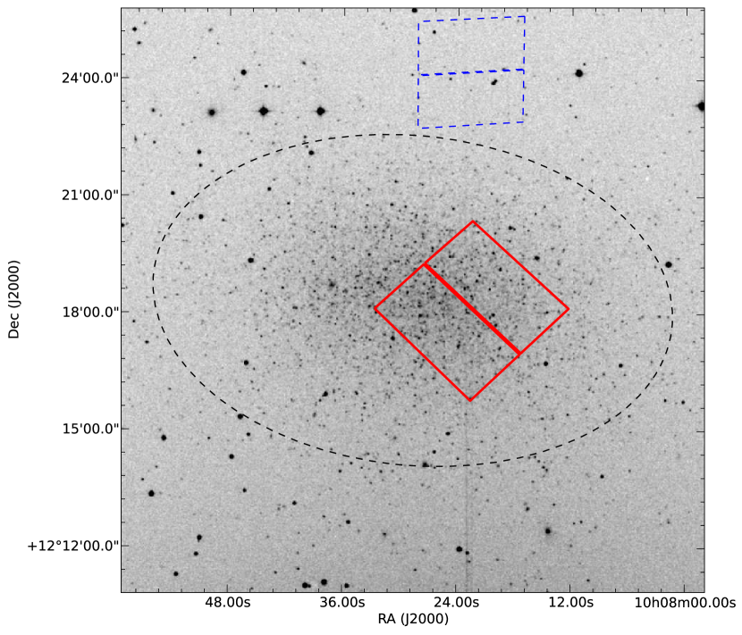
Figure 1.— Field location of our ACS/WFC observations plotted in red over a 15′$\times$15′ section of the sky centered on Leo I from the STScI Digital Sky Survey. The line that bisects the ACS/WFC field is a small gap between two CCDs; the CCD readout direction is roughly perpendicular to this. The dashed ellipse represents the King limiting boundary as derived by Sohn et al. (2007). The parallel WFC3/UVIS field is plotted in blue dashed lines.

The data used in this study to measure the proper motion of Leo I consist of images taken with HST in two different epochs separated by $\sim 5$ years in time. For the first-epoch data, we used the images taken in February 2006 for the science program GO-10520 (PI: T. Smecker-Hane) to study the star formation history of Leo I. A field slightly offset from the center of Leo I was imaged with the ACS/WFC using the F435W and F814W filters. The ACS/WFC covers a field-of-view of $\sim 200"\times 200"$ at a scale of 0.05 arcsec/pixel. Figure 1 shows the field location overlaid on a STScI Digital Sky Survey image centered on Leo I. Sets of 7 and 6 images with exposure times of 1,700 sec each were obtained in F435W and F814W, respectively, and three additional 440 sec F814W images were obtained as well.

The second-epoch data were obtained in January 2011 for our science program GO-12270 (PI: S. Sohn). We pre-analyzed the first-epoch data to enable optimal design of the second-epoch observations. This analysis indicated that the F814W filter provides a slightly better astrometric handle on extended objects than the F435W filter (see also Mahmud & Anderson, 2008, for a discussion of the wavelength dependence of the astrometric accuracy). We therefore took second-epoch observations only with F814W. We obtained 12 images with individual exposure times ranging from 1,267 to 1,364 sec. The resulting total exposure time for the second epoch was $\sim 16$ ksec. Individual exposures were dithered using a pattern designed to optimize the sampling of the point-spread functions (PSFs) for stars that fall on different parts of the detector. This “pixel-phase coverage” is crucial for creating a high-resolution stacked image from a limited number of individual exposures.

We matched the orientation and field center of the second-epoch observations as closely as possible to those of the first-epoch observations. However, due to unavailability of the same guide stars used for the first-epoch observations, we had to use an orientation that differed by $\sim 1$°. We also obtained parallel observations with WFC3/UVIS in the second epoch for an off-target field. This field, also shown in Figure 1, was imaged in F438W and F814W to allow a study of the stellar population in the outer halo of Leo I. However, these observations are not discussed further in the present paper.

2.2. Measurement Technique

To measure the proper motion of Leo I, we compare the two epochs of HST F814W imaging data and determine the average shift of Leo I stars relative to distant background galaxies. This requires a method that allows accurate positions to be measured for both stars and compact galaxies. Mahmud & Anderson (2008) presented a method that accomplishes this by constructing and fitting an individual template for each source in an image. Sohn et al. (2012) implemented, expanded and applied this method to measure the proper motion of the galaxy M31 using HST ACS/WFC and WFC3/UVIS images of three distinct fields imaged over a 5–7 year time baseline. We adopt their method here to also analyze the new Leo I data. We discuss only the main outline and results of the proper motion derivation, and refer the reader to Sohn et al. (2010) and Sohn et al. (2012) for more details about the methodology.

All the science _flt.fits images for the first and second epochs were downloaded from the archive. To each image we first applied the Charge Transfer Efficiency (CTE) correction routine developed by Anderson & Bedin (2010). We then used the img2xym_WFC.09x10 program (Anderson & King, 2006) to determine a position and a flux for each star in each exposure. The positions were subsequently corrected for the known ACS/WFC geometric distortions. Separate distortion solutions were used for the first- and second-epoch data, to account for a difference between pre- and post-SM4 ACS/WFC data (see Section 3.3 of Sohn et al., 2012). We then adopt the first exposure of the second epoch (jbjm01kkq) as the frame of reference. We cross-identify stars in this exposure and the same stars in other exposures. We use the distortion-corrected positions of the cross-identified stars to construct a six-parameter linear transformation between the two frames. These transformations are then used in a program that constructs a stacked image, cleaned of cosmic rays and detector artifacts, of the different exposures in each filter+epoch combination. The stacked images were super-sampled by a factor of 2 relative to the native ACS/WFC pixel scale for better sampling.

Stars and galaxies were identified from the stacked second-epoch F814W image, which provides our deepest view of the field. First, a list of point sources was constructed from the sources detected by img2xym_WFC.09x10. The selection of Leo I stars from this list is relatively straightforward, since our target field is numerically and spatially dominated by Leo I stars (Leo I is located at high Galactic latitude $b=49\arcdeg$, so few foreground stars are expected). To select only bona fide and well-measured Leo I stars, we require: (1) small RMS scatter between the 12 independent position measurements; (2) consistent position in the color-magnitude diagram (obtained from combination with the first-epoch F435W results) with the expected Leo I stellar evolutionary features; and (3) consistent proper motion with the other Leo I stars. This yielded a list of 36,000 stars suitable for proper motion analysis. For the selection of background galaxies in the target field, we started with a candidate list generated by running SExtractor (Bertin & Arnouts, 1996) on the stacked image. From this list we then carefully identified 116 compact background galaxies by eye.

Figure 2.— One-dimensional positional uncertainty per exposure as a function of instrumental magnitude, for Leo I stars (upper panels) and background galaxies (lower panels). The error is defined as $\sigma_{1-D}=\sqrt{\frac{1}{2}({\sigma_{x}}^{2}+{\sigma_{y}}^{2})}$. Here $\sigma_{x}$ and $\sigma_{y}$ are the per-coordinate RMS residuals with respect to the average for the multiple second-epoch measurements. The errors for the first-epoch measurements are slightly larger, but have a similar dependence on instrumental magnitude. All random errors are propagated into our final proper motion measurement for Leo I as described in the text.

For each star/galaxy in each F814W exposure of each epoch we then measured in consistent fashion a position using the template-fitting method. Templates were constructed from the second-epoch stacked image via interpolation. The template-fitting for the first-epoch data included an additional $7\times 7$-pixel convolution kernel, to allow for PSF differences between epochs. This kernel was determined from the data for bright and isolated Leo I stars, without any assumed field-dependence. This is similar to what was done in our analysis of M31 (Sohn et al., 2012), except that in that case the role of the epochs was reversed (since for M31 our first-epoch data were the deepest).

The template-fitted positions were corrected as before for the ACS/WFC geometric distortion. Again, star positions in individual exposures were used to determine six-parameter linear transformations with respect to the first exposure (jbjm01kkq, adopted as the frame of reference) but now using only the selected Leo I stars. These linear transformations were then used to transform the measured positions of all selected stars and background galaxies in all exposures into the reference frame.

The individual exposures lead to multiple determinations for the position of each star or background galaxy in each epoch. We average these determinations to obtain the average position of each source in each epoch. The RMS scatter between measurements in a given epoch quantifies the random positional uncertainty in a single measurement. The error in the mean is smaller by $\sqrt{N}$, where $N$ is the number of exposures in the epoch.

Figure 2 shows the one-dimensional positional errors per second-epoch exposure for Leo I stars (upper panels) and background galaxies (lower panels), as a function of instrumental magnitude (defined as $m_{\rm instr}=-2.5\log[{\rm counts}]$). Brighter objects produce a higher signal-to-noise ratio than fainter objects, and therefore have more accurately determined positions. Stars are more compact than background galaxies, and therefore generally have more accurately determined positions. However, the brightest galaxies have positional uncertainties comparable to those of the brightest stars.

The proper motion of a source is the difference between its average position in the two epochs, divided by the time baseline (4.93 years). By construction, our method aligns the star fields between the two epochs. So with this convention, Leo I stars have zero motion on average, and the background galaxies move over time. Of course, in reality the background galaxies are stationary and the Leo I stars move in the foreground. So the actual average proper motion of Leo I stars is obtained as $-1$ times the measured average proper motion of the background galaxies.

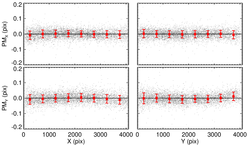
Figure 3.— Displacements of individual stars brighter than instrumental magnitude of $-10$ (dark gray dots) versus detector location between one of the 1,700 sec first-epoch images (j9gz04tsq) and the average of the second-epoch images, plotted separately for $X$ and $Y$ positions. The average and RMS displacements of stars in every 500-pixel bin are shown in red. The displacements average to zero by construction. The scatter is a measure of the per-exposure positional accuracy for a star in this brightness range. Low-level trends are indicative of residual detector effects. The units are in native ACS/WFC pixels, and $X$ and $Y$ positions are in the reference frame.

Figures 3 shows the measured proper motion of each star brighter than instrumental magnitude $-10$ in $X$ and $Y$ as a function of detector coordinates, for one of the 1,700 sec first-epoch images. The motions are zero on average by construction, but there remain small residual trends with position on the detector at levels $\lesssim 0.01$ pixel. This could be due, e.g., to limitations in the adopted geometric distortion corrections. These trends are corrected by measuring the displacement of each background galaxy with respect to only those Leo I stars that lie in the vicinity of the galaxy. This “local correction” removes any remaining systematic proper motion residuals associated with the detector position. Each local correction was constructed using stars of similar brightness ($\pm 1$ mag) and within a 200 pixel region centered on the given background galaxy. The 200 pixel size was chosen to provide a good compromise between having a sufficient number of stars (typically in the range 25-250), and not including too many distant sources.

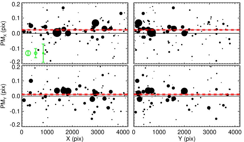
Figure 4.— Displacements of background galaxies versus detector location between one of the 1,700 sec first-epoch images (j9gz04tsq) and the average of the second-epoch images, plotted separately for $X$ and $Y$ positions. The black points show the relative displacements measured for different background galaxies. The weighted average for all galaxies is shown as the red line; dashed red lines indicate the 1-$\sigma$ error region around the average. This region is smaller than the scatter between the points by a factor of $\sim\sqrt{N}$, where $N$ is the number of background galaxies. The radius of each black point is proportional to $1/\Delta$ , where $\Delta$ is the proper motion measurement uncertainty for the particular background galaxy. Hence, the area of each point is proportional to the weight a point receives in the final weighted average. Symbols in green in the top left panel illustrate how the point size relates to the proper motion uncertainty $\Delta$. The units are in native ACS/WFC pixels, and $X$ and $Y$ positions are in the reference frame.

Figure 4 shows the measured proper motion of each background galaxy in $X$ and $Y$ as a function of detector coordinates, for the same 1,700 sec first-epoch image as in Figure 3. The proper motion of each background galaxy is measured with respect to the average second-epoch position of that galaxy, including the local correction. There are far more stars than background galaxies in our images, and star positions are generally determined more accurately than galaxy positions. Hence, the final proper motion uncertainty is dominated by the astrometric accuracy for the background galaxies. For each individual first-epoch exposure we take the weighted average over all background galaxies (larger symbols in Figure 4 denote background galaxies with more accurate measurements, which receive more weight) to obtain a individual Leo I proper motion estimate (red line). The 1-$\sigma$ confidence region around the weighted average (dashed lines) was computed using the bootstrap method (Efron & Tibshirani, 1993), with 10,000 bootstrap samples.

2.3. Inferred Proper Motion

The proper motion diagram for the 9 independent first-epoch measurements is shown in Figure 5. We plot the data points for the longer (1,700 sec; open squares) and shorter (440 sec; open triangles) exposures in the same diagram. We transformed the proper motions and their associated errors along the detector axes to the directions West and North using the orientation of the reference image with respect to the sky ($-47$$\fdg$7). Table 1 lists the proper motion for each first-epoch image and the corresponding error, along with the number of background galaxies used for the proper motion derivation.

The final average proper motion of Leo I is calculated by taking the error-weighted mean of the 9 independent measurements listed in Table 1. This yields

$$(\mu_{W},\mu_{N})=(0.1140\pm 0.0295,-0.1256\pm 0.0293)\ {\rm mas\ yr}^{-1}.$$ (1)

This result differs from zero at approximately 4-$\sigma$ confidence in each coordinate direction, so the detected motion of Leo I is very statistically significant.

The quantity

$$\chi^{2}=\sum_{i}\left[\left(\frac{\mu_{W,i}-{\overline{\mu}_{W}}}{\Delta\mu_{W,i}}\right)^{2}+\left(\frac{\mu_{N,i}-{\overline{\mu}_{N}}}{\Delta\mu_{N,i}}\right)^{2}\right]$$ (2)

provides a measure of the extent to which different measurements agree to within the random errors. In absence of systematic errors, one expects that this quantity follows a $\chi^{2}$ probability distribution with $N_{DF}=18-2=16$ degrees of freedom. The expectation value for such a distribution is $N_{DF}$, and the dispersion is $\sim\sqrt{2N_{DF}}=5.7$. We find $\chi^{2}=11.2$ for our measurements. This indicates that the measurements from the different exposures are consistent, and that the errors may actually be slight overestimates.

The final Leo I proper motion uncertainties correspond to $\sim 29\ \mu$as yr^-1. This is a factor of $>2$ larger than what we achieved for M31 (Sohn et al., 2012), due mostly to the fact that for M31 deeper exposures were available for three different fields. Our M31 HST measurements approached the accuracy achieved using VLBA water maser observations for the M31 satellites M33 and IC10. Whereas this is not the case here, our Leo I measurements are more accurate than what has been achieved with HST for other MW satellites, using one or more fields centered on background quasars (see the compilation in Table 4 of Watkins et al., 2010).

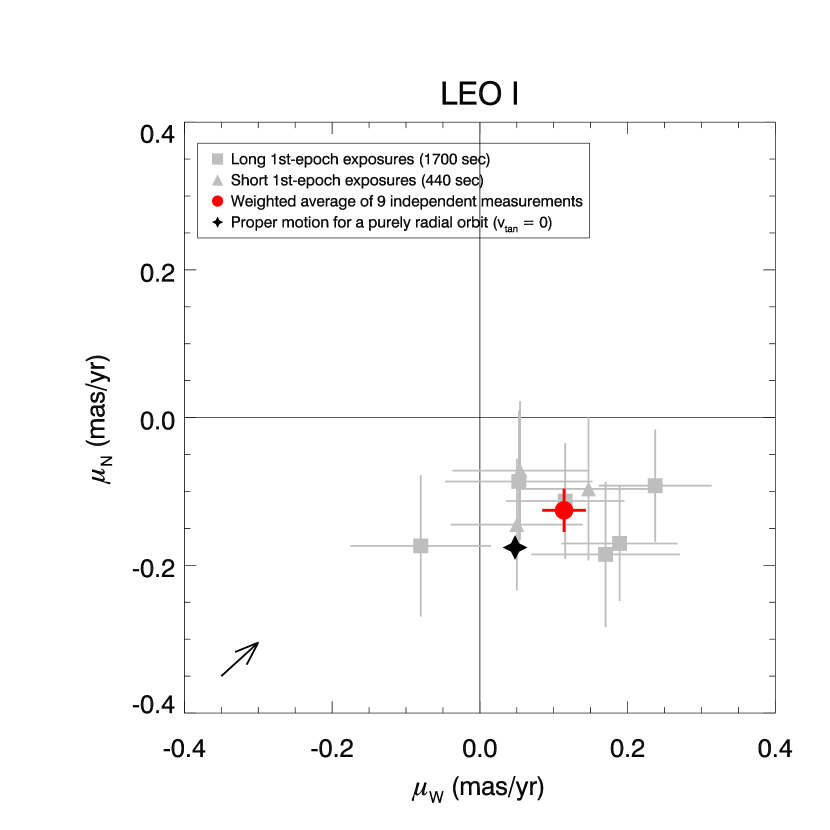
Figure 5.— Leo I proper motion results. Each gray dot with an error bar indicates the average proper motion of Leo I stars inferred from a single first-epoch exposure. Measurements using images with longer (closed square) and shorter (closed triangle) exposure times are indicated with different symbols. The solid red data point is the weighted average of the nine separate measurements, which is the final result of our analysis. The origin corresponds to the velocity such that Leo I has no transverse motion in the heliocentric rest frame. The star symbol corresponds to the velocity such that Leo I has no tangential velocity in the Galactocentric rest frame (i.e., a radial orbit with respect to the MW). The line segment in the bottom left corner indicates the CCD $Y$-direction. The two ACS/WFC CCDs are read out in the $\pm Y$-directions, respectively.

Table 1Proper Motion Results

	$\mu_{W}$	$\mu_{N}$
Data Set	(mas yr-1)	(mas yr-1)	$N_{\rm used}$
j9gz04tsq	+0.2374 $\pm$ 0.0763	$-$0.0922 $\pm$ 0.0759	100
j9gz04ttq	+0.1156 $\pm$ 0.0801	$-$0.1129 $\pm$ 0.0784	101
j9gz04tvq	+0.1892 $\pm$ 0.0785	$-$0.1704 $\pm$ 0.0779	090
j9gz05tyq	+0.1702 $\pm$ 0.1003	$-$0.1853 $\pm$ 0.0984	096
j9gz05tzq	$-$0.0800 $\pm$ 0.0950	$-$0.1737 $\pm$ 0.0957	086
j9gz05u1q	+0.0528 $\pm$ 0.0996	$-$0.0865 $\pm$ 0.0962	098
j9gz06krq	+0.1471 $\pm$ 0.0977	$-$0.0966 $\pm$ 0.0970	056
j9gz06ksq	+0.0545 $\pm$ 0.0917	$-$0.0718 $\pm$ 0.0939	053
j9gz06kuq	+0.0501 $\pm$ 0.0894	$-$0.1449 $\pm$ 0.0891	054
weighted av.	+0.1140 $\pm$ 0.0295	$-$0.1256 $\pm$ 0.0293

2.4. Control of Systematic Errors

The technique used here for measuring proper motions is identical to that used in our study of M31, as described in Sohn et al. (2012). As discussed in detail in section 4.3 of that paper, the technique has many built-in features to minimize the impact of systematic errors on the measurement. For example, we explicitly correct for Y-CTE using the technique of Anderson & Bedin (2010), we use different geometric distortion solutions for the two epochs, and we model PSF variations between epochs. Moreover, any remaining astrometric residuals from these instrumental effects will have very limited impact on our proper motion measurement. This is because our measurement is a differential one between stars and background galaxies, observed at the same time on the same detector. Through our local correction, we restrict the differential comparison to sources of similar magnitude observed on the same part of the detector. This effectively minimizes both geometric distortion and PSF residuals (which depend on detector position) and CTE-residuals (which depend on detector position and source magnitude). Also, our final random proper motion errors in Table 1 are calculated through bootstrapping, which means that they reflect the scatter between results from different background galaxies. Any systematic proper motion residuals that vary with position on the detector (e.g., from CTE) are therefore accounted for in the random errors.

Despite our best efforts, there will always be some remaining level of systematic error in the final proper motion measurement. This could be, e.g., from the fact that the astrometric CTE impact is different for point sources and extended sources, from the fact that we have not explicitly corrected for X-CTE (which is only $\sim 1$% of the size of Y-CTE), from color-difference effects, or from other higher-order effects. In the context of our M31 proper motion study, we therefore set up the observational experiment such that we would have several independent limits on the size of any remaining systematic errors: (1) we observed an object for which an entirely independent estimate exists of the transverse velocity (van der Marel & Guhathakurta, 2008); (2) we observed with two different instruments (ACS/WFC and WFC3/UVIS) for the second epoch; and (3) we chose to observe, at different times and with different telescope orientation, three well-separated fields, which have different types and numbers of background galaxies, and different level of stellar densities. We found that different methods, different instruments, and different fields, all yielded proper motion answers with our HST technique that are statistically consistent. Fig. 13 of Sohn et al. (2012) and Fig. 3 van der Marel et al. (2012a) show that there is agreement to better than $\sim 100$ km/s, which at the distance of M31 corresponds to $0.027$ mas/yr. This scatter can be attributed entirely to known random errors, and this therefore sets a rigorous and conservative upper limit to any possible systematic errors in our technique.

Since systematic errors in our technique had been previously validated, we did not set up our Leo I experiment to provide a similar level of independent systematic error validation. For efficiency of HST usage, we observed only one field, with one instrument. However, our setup is otherwise very similar to in our M31 study: we again compare two epochs of ACS/WFC data, one taken before the Service Mission 4 (SM4) and the other after the SM4, with a 5 year time baseline. Therefore, any remaining systematic proper errors in our Leo I result should be similar to what was present in the M31 result, and that was rigorously and conservatively bounded by $0.027$ mas/yr. This is below the random error in our Leo I result. Therefore, any systematic errors in our result should be below the quoted random error.

We also performed a variety of additional tests on our Leo I data to confirm that indeed no unidentified systematics are present. We did not find any dependence of the proper motions of the stars and background galaxies in the field on $I$-magnitude, $B-I$ color, or source extent (FWHM). Using a different magnitude range in the local corrections didn’t change the final proper motion result by more than the random errors. Comparing results for background galaxies near to and far from the read-out amplifiers yielded consistent results given the the uncertainties: when using only galaxies close to the amplifiers (i.e., limited CTE losses), our results change to $(\mu_{W},\mu_{N})=(0.0875\pm 0.0392,-0.1703\pm 0.0390)\ {\rm mas\ yr}^{-1}$, while using only galaxies far from the amplifiers (i.e., higher CTE losses), our results changed to $(\mu_{W},\mu_{N})=(0.1467\pm 0.0403,-0.0504\pm 0.0396)\ {\rm mas\ yr}^{-1}$. These results differ from our final PM results (Equation 1) by (0.7$\sigma$, 1.1$\sigma$) and (0.8$\sigma$, 1.9$\sigma$), respectively. As a test, we also reduced the data without inclusion of the Anderson & Bedin (2010) pixel-space CTE correction. This is clearly wrong, since we know that CTE is present and well-corrected by this correction, but even this only changed the final proper motion result by an average of $1.5$ times the random error per coordinate. So overall, we have no reason to believe that any systematic errors are present in our final proper motion result at a level that exceeds the quoted random errors.

3. The Orbit of Leo I

3.1. Velocity in the Galactocentric Rest Frame

We adopt a Cartesian Galactocentric coordinate system ($X,Y,Z$), with the origin at the Galactic Center, the $X$-axis pointing in the direction from the Sun to the Galactic Center, the $Y$-axis pointing in the direction of the Sun’s Galactic rotation, and the $Z$-axis pointing towards the Galactic North Pole. The position and velocity of an object in this frame can be determined from the observed sky position, distance, line-of-sight velocity, and proper motion, as in, e.g., van der Marel et al. (2002).

To determine the Galactocentric position of an object, it is necessary to also know the distance $R_{0}$ of the Sun from the Galactic Center. Moreover, it is necessary to know the velocity of the Sun inside the MW to turn observed heliocentric rest-frame velocities into Galactocentric rest-frame velocities. Following van der Marel et al. (2012a), we adopt the recent values of McMillan (2011) for the distance of the Sun from the Galactic center and the circular velocity of the local standard of rest (LSR): $R_{0}=8.29\pm 0.16$ kpc and $V_{0}=239\pm 5$ km s^-1. For the solar peculiar velocity with respect to the LSR we adopt the estimates of Schönrich et al. (2010): $(U_{\rm pec},V_{\rm pec},W_{\rm pec})=(11.10,12.24,7.25)$ km s^-1 with uncertainties of $(1.23,2.05,0.62)$ km s^-1.

To obtain the distance of Leo I, we average the distances measured via the tip of the red-giant branch (TRGB) method in the last decade (Méndez et al., 2002; Bellazzini et al., 2004; Held et al., 2010), which yields $256.7\pm 13.3$ kpc. This implies a Galactocentric $(X,Y,Z)$ position

$${\vec{r}}=(-125.0,-120.8,194.1)\>{\rm kpc},$$ (3)

with an uncertainty of 13.3 kpc along the line-of-sight direction.

The most recent measurement of the systemic heliocentric line-of-sight velocity of Leo I is $v_{\rm LOS}=282.9\pm 0.5$ km s^-1 (Mateo et al., 2008). The measured proper motion $\mu$ from equation (1) corresponds to a heliocentric transverse velocity in km/s equal to $4.7404\times D({\rm kpc})\times\mu({\rm mas\ yr}^{-1})$. This implies

$$(v_{W},v_{N})=(138.7\pm 36.6,-152.8\pm 36.5)\>{\rm km}\,{\rm s}^{-1}$$ (4)

with proper motion errors dominating over distance errors in the determination of the velocity errors. The internal velocity dispersion of Leo I is $\sigma=9.2\pm 0.4\>{\rm km}\,{\rm s}^{-1}$, with little evidence for rotation (Mateo et al., 2008). This is well below our observational velocity errors. Hence, there is no need to correct the observed values for the internal kinematics of Leo I, even though our field was offset from its photometric center (see Figure 1).

The velocity for which Leo I would be on a radial orbit with respect to the MW (i.e., the velocity for which there is zero tangential velocity in the Galactocentric rest frame) is

$$(v_{W},v_{N})_{\rm rad}=(58.0,-214.0)\>{\rm km}\,{\rm s}^{-1}.$$ (5)

This differs from the measured proper motion at almost 3-$\sigma$ significance. Therefore, our measurements imply that Leo I is not on a radial orbit about the MW.

Several authors have argued previously that the Galactocentric tangential velocity of Leo I is probably small, given its significant radial velocity (Byrd et al., 1994; Sohn et al., 2007; Mateo et al., 2008). Indeed, Figure 5 shows that the observed proper motion does fall in the same quadrant of proper motion space as a radial orbit. This can be interpreted as a consistency/plausibility check on the proper motion measurement. The same was found for the case of M31, for which we also presented several other successful consistency checks on our proper motion analysis methodology (Sohn et al., 2012).

Conversion into the Galactocentric rest frame yields for the velocity vector of Leo I

$${\vec{v}}=(-167.7\pm 31.9,-37.0\pm 33.0,94.4\pm 24.2)\>{\rm km}\,{\rm s}^{-1}.$$ (6)

The listed uncertainties here and hereafter were obtained from a Monte-Carlo scheme that propagates all observational distance and velocity uncertainties and their correlations, including those for the Sun. Note that the Galactocentric velocity uncertainties are highly correlated because the observational velocity uncertainty is much larger in the transverse direction than in the line-of-sight direction.

The corresponding Galactocentric radial and tangential velocities are

$$(V_{\rm rad},V_{\rm tan})=(167.9\pm 2.8,101.0\pm 34.4)\>{\rm km}\,{\rm s}^{-1}.$$ (7)

Although the tangential velocity is significantly non-zero, it is less than the radial velocity. So while Leo I is not on a radial orbit about the MW, the orbit must be fairly elliptical. The observed total Leo I velocity with respect to the MW is

$$v\equiv|{\vec{v}}|=196.0\pm 19.4\>{\rm km}\,{\rm s}^{-1}$$ (8)

with the listed numbers corresponding to the peak and the symmetrized 1$\sigma$ of the $v$ probability distribution.

These inferred Leo I velocities use a solar velocity inside the MW based on Schönrich et al. (2010) and McMillan (2011), which yields an azimuthal velocity component $v_{\phi,\odot}=251.2\>{\rm km}\,{\rm s}^{-1}$. However, alternative values for the solar velocity continue to be in common use. These differ from the values used here primarily in the azimuthal direction. For example, with the old IAU recommended circular velocity $V_{0}=220\>{\rm km}\,{\rm s}^{-1}$ and the peculiar velocities from Dehnen & Binney (1998), $v_{\phi,\odot}=225.2\>{\rm km}\,{\rm s}^{-1}$. Based on these latter values, the Galactocentric Leo I velocities would be $V_{\rm rad}=180.5\>{\rm km}\,{\rm s}^{-1}$, $V_{\rm tan}=93.8\>{\rm km}\,{\rm s}^{-1}$, and $v=203.4\>{\rm km}\,{\rm s}^{-1}$, which can be compared to the values in equations (7) and (8). While the change in $V_{\rm rad}$ is significant compared to the small uncertainties, $V_{\rm tan}$ and $v$ change by much less than the observational uncertainties. The conclusions of the present paper and Paper II are therefore not very sensitive to the adopted solar velocity. The value of $v_{\phi,\odot}$ assumed here is consistent with the recent determination of $v_{\phi,\odot}=242_{-3}^{+10}\>{\rm km}\,{\rm s}^{-1}$ by Bovy et al. (2012), while the alternative $v_{\phi,\odot}=225.2\>{\rm km}\,{\rm s}^{-1}$ discussed above is not.

3.2. Keplerian Orbit Calculations

To assess the implications of the new measurements, we start with the assumption that the MW can be approximated as a point mass, and that Leo I orbits in its potential as a test particle on a Keplerian orbit. The assumption of a Keplerian potential for the MW is not as unreasonable as it may seem at first. The large Galactocentric distance of Leo I, $r\equiv|{\vec{r}}|=260.6$ kpc, combined with its significant tangential velocity, implies that much of the MW’s mass is inside the Leo I orbit at all times. We calculate models with more realistic MW potentials in Section 3.3.

The escape velocity for a point mass $M_{\rm MW}$ is

$$v_{e}=\sqrt{2GM_{\rm MW}/r}.$$ (9)

Hence, given the observed total Leo I velocity with respect to the MW given by equation (8), Leo I is bound to the MW if $M_{\rm MW}\geq(1.16\pm 0.24)\times 10^{12}{M_{\odot}}$. Cosmological simulations imply that it is very unlikely to find an unbound satellite at the present epoch near a MW-type galaxy (e.g., Deason et al., 2011, and Paper II). So if we assume that Leo I must be bound to the MW, then this can be interpreted as a new crude lower limit on the MW mass.

Alternatively, one may assume that the mass of the MW is already constrained from other arguments. In that case, one can use the new measurement to assess the probability that Leo I is in fact bound. Studies of the MW mass have advocated many different values, roughly covering the range $0.75$–$2.25\times 10^{12}{M_{\odot}}$ (see Boylan-Kolchin et al., 2012, for a compilation of recent mass estimates of the MW). van der Marel et al. (2012a) assumed a flat prior probability over this range, and then used a Bayesian scheme to include the latest measurements of the Local Group timing mass, based on our M31 HST proper motion work. The Local Group timing mass is relatively high, which increases the likelihood of high MW masses compared to low MW masses. We combined the probability distribution for the MW mass from Figure 4 of van der Marel et al. (2012a) with the measured $v$ for Leo I. This implies that there is a 77% probability that Leo I is bound to the MW, and a 23% probability that it is not bound. The preference for a bound state is consistent with expectations from cosmological simulations (e.g., Benson, 2005; Wetzel, 2011).

For any assumed point mass $M_{\rm MW}$, and given Galactocentric Leo I phase-space vectors ${\vec{r}}$ and ${\vec{v}}$, the shape of the Keplerian orbit is determined analytically. We calculated these orbits in a Monte-Carlo sense. At each Monte-Carlo step we draw a mass $M_{\rm MW}$ from the previously discussed probability distribution derived by van der Marel et al. (2012a), and we draw Leo I phase-space vectors from the observationally determined values and uncertainties. We then determine the statistics of the orbital characteristics over the Monte-Carlo sample.

The Monte-Carlo analysis yields an average ratio of pericenter to apocenter distance $r_{\rm peri}/r_{\rm apo}=0.06\pm 0.03$ for the bound elliptical Keplerian orbits (i.e., orbits with eccentricity of less than 1). Leo I has a positive radial velocity, and is therefore past pericenter. The pericentric passage occurred at $t_{\rm peri}=1.18\pm 0.45$ Gyr ago at a Galactocentric distance of $r_{\rm peri}=67\pm 39$ kpc. The velocity at pericenter was $v_{\rm peri}=561\pm 475\>{\rm km}\,{\rm s}^{-1}$. The uncertainties in these quantities are determined largely by the uncertainties in the Leo I phase-space vectors, and much less so by uncertainties in MW mass. For example, if $M_{\rm MW}$ is kept fixed at $1.5\times 10^{12}{M_{\odot}}$ for all Monte Carlo drawings, then the orbital characteristics become: $r_{\rm peri}/r_{\rm apo}=0.04\pm 0.02$, $t_{\rm peri}=1.08\pm 0.13$ Gyr, $r_{\rm peri}=69\pm 38$ kpc, $v_{\rm peri}=518\pm 417\>{\rm km}\,{\rm s}^{-1}$. In Section 3.3 we compare these simple Keplerian results to the results from orbit calculations in more detailed cosmologically-motivated halo models.

Another useful application of Keplerian orbits is through the timing argument (Kahn & Woltjer, 1959). This argument assumes that bound galaxy pairs follow a Newtonian Keplerian trajectory starting soon after the Big Bang, which corresponds to the “first pericenter.” The galaxies initially move away from each other due to the expansion of the Universe, but then fall back towards each other due to gravity. In this picture, Leo I is just passed its second pericenter. In general, there are four observables (the time since Big Bang $t$, relative distance $r$, radial velocity $V_{\rm rad}$, and tangential velocity $V_{\rm tan}$) and four independent orbital parameters (eccentric anomaly $\eta$, semi-major axis length $a$, eccentricity $e$, and the total mass $M$). Hence, the Keplerian orbit can be solved for analytically, as described in e.g., van der Marel & Guhathakurta (2008). One may call this the “complete timing argument” (cta). In many applications however, the transverse velocity $V_{\rm tan}$ is not known and it is then often assumed that $V_{\rm tan}=0$ and $e=1$. This yields the so-called “radial-orbit timing argument” (rta).

The timing argument has traditionally been applied to the MW–M31 system (see van der Marel et al., 2012a, and references therein), but it can also be applied to the MW–Leo I system (Zaritsky et al., 1989). The radial-orbit timing argument as applied to Leo I with the previously derived Galactocentric position and velocity implies a mass $M_{\rm MW,rta}=(1.50\pm 0.12)\times 10^{12}{M_{\odot}}$ (consistent with the value previously inferred by Li & White, 2008, using a slightly different assumed solar velocity). Any tangential velocity increases the timing mass. Since we have now measured the tangential velocity of Leo I, we can use instead the complete timing argument without assuming a radial orbit. This implies a mass $M_{\rm MW,cta}=(1.93\pm 0.42)\times 10^{12}{M_{\odot}}$.

The error bars in the listed timing masses reflects only the propagation of errors in the observational quantities. However, it is important to also quantify any inherent biases and cosmic scatter, and to calibrate the timing mass to more traditional measures of mass, such as the virial mass. Li & White (2008) addressed these issues for the radial-orbit timing argument using the cosmological Millennium simulation. They identified a set of host galaxy - satellite pairs with properties similar to the MW-Leo I pair. For these pairs they studied the statistics of the ratio $M_{\rm 200}/M_{\rm rta}$. In the following we find it more convenient to use the virial mass $M_{\rm vir}$ rather than the quantity $M_{\rm 200}$, so where necessary we transform the latter to the former using $M_{\rm vir}/M_{200}=1.19$ (as appropriate for an NFW halo of concentration $c=9.5$; see the Appendix of van der Marel et al., 2012a, for the relevant equations and mass definitions).

Yang-Shyang Li kindly made available the catalog of galaxy pairs used in the analysis of Li & White (2008) (the sample defined by the bottom row of their Table 3). This allowed us to perform an analysis similar to theirs, but now for the complete timing argument. We find that the bias $M_{\rm vir}/M_{\rm cta}=1.46_{-0.62}^{+0.89}$. This estimate was obtained, as in the Li & White (2008) analysis, by averaging over all satellites in the simulation sample, independent of tangential velocity. However, we have now measured the tangential velocity of Leo I. So we can get a more appropriate measure of the bias by including only the satellites with tangential velocities similar to that of Leo I. If we require agreement in $V_{\rm tan}$ to within $25\>{\rm km}\,{\rm s}^{-1}$, we find that $M_{\rm vir}/M_{\rm cta}=1.63_{-0.61}^{+0.74}$. For comparison, this same selection yields for the radial-orbit timing argument that $M_{\rm vir}/M_{\rm rta}=2.10_{-0.69}^{+0.95}$. So the complete timing argument yields estimates of $M_{\rm vir}$ that are biased low, but not by as much as the radial orbit timing argument. This is because part of the bias is due to the fact that satellite galaxies generally have non-zero tangential velocities, and this is explicitly taken into account in the complete timing argument.

These results for cosmic bias and scatter can be combined with the previously inferred values of $M_{\rm MW,cta}$ and $M_{\rm MW,rta}$. This yields $M_{\rm MW,vir}=3.15_{-1.36}^{+1.58}\times 10^{12}{M_{\odot}}$ from the complete timing argument, and $M_{\rm MW,vir}=3.14_{-1.06}^{+1.45}\times 10^{12}{M_{\odot}}$ from the radial-orbit timing argument, respectively. So the two timing arguments give similar results and uncertainties. The mass estimates are higher than most MW mass estimates based on other methods (consistent with the results of Li & White, 2008), but they are probably not inconsistent with other MW mass estimates given the significant cosmic scatter. This situation is similar to what was found for MW mass estimates based on the timing of the MW-M31 system (van der Marel et al., 2012a).

3.3. Detailed Orbit Integrations

3.3.1 Methodology & Overview

To get a better understanding of the past orbital history of Leo I we need to use more detailed models for the MW’s gravitational potential $\Phi_{\rm MW}$. Following Besla et al. (2007), we describe this potential as a static, axisymmetric, three-component model consisting of dark matter (DM) halo, disk (Miyamoto & Nagai, 1975) and stellar bulge (Hernquist, 1990):

$$\Phi_{\rm MW}=\Phi_{\rm DM~{}halo}+\Phi_{\rm disk}+\Phi_{\rm bulge}.$$ (10)

The DM halo is initially modeled as an NFW halo (Navarro et al., 1997) with a virial concentration parameter ($c_{\rm vir}$) defined as in Klypin et al. (2011) from the Bolshoi Simulation (see also, van der Marel et al., 2012b). We apply the adiabatic contraction of the NFW halo in response to the slow growth of an exponential disk using CONTRA code (Gnedin et al., 2004). The density profile of the MW is then truncated at the virial radius . The bulge mass of the MW is kept fixed at $10^{10}{M_{\odot}}$ with a Hernquist scale radius of 0.7 kpc. The exponential disk scale length is also kept fixed at 3.5 kpc.

We adopt three different mass models for the MW with total virial masses of $1.0\times 10^{12}$, $1.5\times 10^{12}$, and $2.0\times 10^{12}{M_{\odot}}$. In all cases, the bulge is modeled with a scale radius of 0.7 kpc and a total mass of $10^{10}{M_{\odot}}$. The disk scale radius is also kept fixed at 3.5 kpc, but the disk mass is allowed to vary to reproduce the circular velocity at the Solar circle. We adopt a MW circular velocity of 239 km s^-1 at the solar radius of 8.29 kpc (McMillan, 2011). Model parameters are listed in Table 2.

Table 2Model Parameters for the Milky Way

$M_{\rm vir}$		$R_{\rm vir}$	$M_{\rm disk}$
(${M_{\odot}}$)	$c_{\rm vir}$	(kpc)	(${M_{\odot}}$)
$1.0\times 10^{12}$	9.86	261	$6.5\times 10^{10}$
$1.5\times 10^{12}$	9.56	299	$5.5\times 10^{10}$
$2.0\times 10^{12}$	9.36	329	$5.0\times 10^{10}$

The escape velocities at the distance $r=260.6$ kpc of Leo I are $182$, $222$, and $256\>{\rm km}\,{\rm s}^{-1}$ for the models with masses of $1.0\times 10^{12}$, $1.5\times 10^{12}$, and $2.0\times 10^{12}{M_{\odot}}$, respectively. For the latter two models, this exceeds our best estimate $v=196.0\pm 19.4\>{\rm km}\,{\rm s}^{-1}$ for the total Galactocentric velocity of Leo I. So Leo I is most likely bound to the MW if $M_{\rm MW,vir}\gtrsim 1.5\times 10^{12}{M_{\odot}}$, as already suggested in Section 3.2. For the lowest-mass MW model studied here, with $M_{\rm MW,vir}=1.0\times 10^{12}{M_{\odot}}$, Leo I is on an unbound hyperbolic orbit. This has repercussions for the viability of such low mass MW models in a cosmological context, since satellites are rarely found on hyperbolic orbits. We explore this in more detail in Paper II.

Using the current Galactocentric position and velocity vectors of Leo I as initial conditions, we can solve the differential equations of motion numerically to follow the velocity and position of Leo I backward in time. If we consider only the gravitational influence of the MW, the equation of motion has the form:

$$\ddot{\boldsymbol{r}}=\frac{\partial}{\partial\boldsymbol{r}}\Phi_{\rm MW}(|\boldsymbol{r}|),$$ (11)

In Section 3.3.2 this equation of motion is solved using well-established numerical methods in order to constrain Leo I’s interaction history with the MW (i.e., pericentric distance and epoch of accretion) over a Hubble time. Leo I is modeled as a Plummer potential with a softening length of 0.5 kpc, and total mass of $1.3\times 10^{8}{M_{\odot}}$ (see Table 3). With these parameters, the dynamical mass of Leo I within 0.93 kpc is $8.9\times 10^{7}{M_{\odot}}$, as expected from Table 2 of Walker et al. (2009) (i.e. the inferred mass within the outermost data point of the empirical velocity dispersion profile, referred to as $r_{\rm last}$ in Walker et al. 2009). We note that dynamical friction is expected to be negligible for such a low mass satellite (even when its extended dark mass outside the outermost data point is included) and it is thus not computed in the equation of motion.

Table 3Properties of Local Group Galaxies

	$M_{\rm total}$	$K$	$r_{\rm last}$	$M(<r_{\rm last})$	$X$	$Y$	$Z$	$V_{X}$	$V_{Y}$	$V_{Z}$	Ref.
Galaxy	(${M_{\odot}}$)	(kpc)	(kpc)	(${M_{\odot}}$)	(kpc)	(kpc)	(kpc)	(km s-1)	(km s-1)	(km s-1)	Dist.	RV	PM
Leo I	$1.30\times 10^{8}$0	00.5	0.93	$8.9\times 10^{7}$0	$-$125.0	$-$120.8	+194.1	$-$167.7	0$-$37.0	+094.4	1,2,3	4	This study
Carina	$5.70\times 10^{7}$0	00.5	0.87	$3.7\times 10^{7}$0	0$-$24.8	0$-$94.8	0$-$39.3	0$-$72.9	+006.9	+038.0	2,5	6	7
Draco	$3.90\times 10^{8}$0	00.5	0.92	$2.6\times 10^{8}$0	00$-$3.5	0+76.3	+053.0	+017.1	+056.0	$-$227.9	8	9	10
Fornax	$1.45\times 10^{8}$0	00.5	1.70	$1.3\times 10^{8}$0	0$-$40.0	0$-$49.2	$-$129.4	0$-$24.5	$-$140.7	+106.2	5,11,12,13,14,15	16	17
Leo II	$6.40\times 10^{7}$0	00.5	0.42	$1.7\times 10^{7}$0	0$-$77.3	0$-$58.3	+215.3	+102.2	+237.0	+118.4	18,19	20	21
Sculptor	$1.35\times 10^{8}$0	00.5	1.10	$1.0\times 10^{8}$0	00$-$5.3	00$-$9.6	0$-$84.1	0$-$19.4	+224.6	$-$101.6	13,22	23	24
Sextans	$2.90\times 10^{7}$0	00.5	1.00	$2.0\times 10^{7}$0	0$-$40.0	0$-$63.6	+064.6	$-$181.1	+113.6	+113.6	25	26	27
Ursa Minor	$7.70\times 10^{7}$0	00.5	0.74	$4.4\times 10^{7}$0	0$-$22.2	+052.1	+053.6	$-$107.5	0$-$15.2	$-$116.1	8	9	28
LMC	$5.00\times 10^{10}$	11.0	9.00	$1.3\times 10^{10}$	00$-$1.1	0$-$41.0	0$-$27.8	0$-$57.4	$-$225.6	+220.7	29	30	31
M31	See text	$\cdots$	$\cdots$	$\cdots$	$-$378.9	+612.7	$-$283.1	+066.1	0$-$76.3	+045.1	32	33	34

Other members in the Local Group with significant masses may exert dynamical influence on the orbital history of Leo I. Relevant to our analysis are the LMC and M31. It has been theorized that a number of satellite galaxies of the MW lie in a similar orbital plane as the Magellanic Clouds, referred to as the “Magellanic Plane” of galaxies (Kunkel & Demers, 1976; Lynden-Bell, 1976). The ubiquity of this statement is directly relevant to cosmological studies of how satellite galaxies are accreted by MW mass halos (e.g., D’Onghia & Lake, 2008; Metz et al., 2009; Sales et al., 2011; Wang et al., 2013). The Sagittarius dSph is known to be orbiting in a plane that is perpendicular to that of the Magellanic Clouds (which orbit approximately in the $Y-Z$ Galactocentric plane). As such, it is clear that at least one of the MW satellites is an outlier. Without accurate proper motions, it has been unclear to what extent Leo I’s orbit lies in a different plane or has a different rotational sense. Furthermore, the Keplerian orbit analysis of Section 3.2 demonstrates that Leo I is likely on a fairly eccentric orbit. On such a high eccentricity orbit, it is possible that M31 may exert an important gravitational influence at early times.

In Section 3.3.4 we compute the orbital histories of the LMC and M31 in addition to that of Leo I to define its orbital plane relative to that of the LMC and also to assess the dynamical significance of M31 to its orbital history and origin. We modify the equations of motion (Eq. 11) to include the gravitational influence of both M31 and the LMC while computing the orbital history of Leo I over the past 8 Gyr. We simultaneously compute the equations of motion for each of the MW, M31 and LMC, accounting for the gravitational acceleration from the other bodies. The orbits are computed in the Galactocentric frame, using the current velocities and positions of the LMC (Kallivayalil et al., 2013) and M31 (van der Marel et al., 2012a), as listed in Table 3. The masses of the MW and M31 are assumed to be static over time, which limits the accuracy of this analysis past 6 Gyr (i.e., when the mass of these galaxies is expected to be about half of their current value, e.g. Fakhouri et al., 2010).

M31 is modeled using an NFW halo, where its virial mass is determined by preserving the total mass of the Local Group, given the mass of the MW in each model. The density profile of M31 is also modeled to be truncated at the virial radius. Using the recent proper motions of M31 by Sohn et al. (2012) and other mass arguments in the literature, van der Marel et al. (2012a) estimate the Local Group mass to be $M_{\rm LG}=(3.17\pm 0.57)\times 10^{12}{M_{\odot}}$. In this analysis we thus require that the combined $M_{\rm MW}+M_{\rm M31}=3\times 10^{12}{M_{\odot}}$. Given the large distances involved, the contribution of M31’s disk/bulge component to the gravitational influence on Leo I is irrelevant.

The LMC is modeled as a Plummer sphere with a softening parameter of 11 kpc and total mass of $5\times 10^{10}{M_{\odot}}$. With these parameters, the mass contained within 9 kpc is $\sim 1.3\times 10^{10}{M_{\odot}}$, as observed (van der Marel et al., 2002). To model the orbital evolution of a massive satellite such as the LMC accurately, dynamical friction effects owing to its motion through the dark matter halo of the MW must be accounted for. Dynamical friction is included using the Chandrasekhar formula with an approximation to the Coulomb logarithm as in Besla et al. (2007). Meanwhile, dynamical friction is irrelevant to the motion of the MW and M31 because their halos do not overlap over the past 8 Gyr.

The star formation history of Leo I has been the topic of many studies, especially with HST (Caputo et al., 1999; Gallart, 1999; Dolphin, 2002; Smecker-Hane et al., 2010). From the most recent HST ACS/WFC observations (Smecker-Hane et al., 2010), Leo I is known to have formed stars continuously since $>12$ Gyr ago, with two pronounced star formation activities at $\sim 4.5$ and $\sim 2$ Gyrs ago. After this last activity, star formation abruptly dropped until a complete cessation at $\sim 0.5$ Gyr ago. Some of the inferred increases and decreases in star formation activity may be related to features in Leo I’s orbit about the MW, including the time of accretion and the pericenter time. We determine these times in Section 3.3.2.

The origin of enhanced star formation activities in Leo I’s past may also be related to interaction with other satellites. Furthermore, three-body encounters may also alter the orbital trajectory of Leo I as proposed by Mateo et al. (2008), potentially explaining its high speed today (e.g., Sales et al., 2007). To test for possible interactions with other MW satellites, we extend in Section 3.3.5 the analysis of Section 3.3.2 such that the equations of motion now account for gravitational interaction terms with the following satellites for which proper motions are available from other studies (see Table 3): Carina, Draco, Fornax, Leo II, Sculptor, Sextans, Ursa Minor, and the LMC. The Sagittarius dSph is not included in this analysis because its orbit is too close to the MW disk plane to dynamically influence that of Leo I. The SMC is also not included because its orbit is likely closely matched to that of its binary companion, the LMC. Since the LMC is the more massive of the pair, it is likely to be the more significant perturber. Each satellite is modeled as a Plummer potential with total mass and softening parameters as listed in Table 3; model parameters are chosen to match the observed masses within $r_{\rm last}$, as defined in Walker et al. (2009).

3.3.2 Leo I Orbital Properties

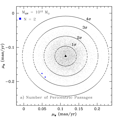
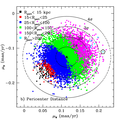
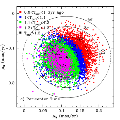
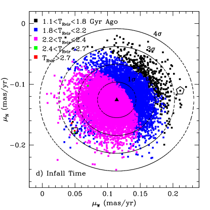
Figure 6.— Ten thousand points randomly sampled from the 4$\sigma$ proper-motion error space of Leo I. The dashed ellipses indicate the standard deviation of the enclosed points from the mean (filled triangle). For each point, the orbital history of Leo I was computed by integrating the equations of motion [equation (11)] backward in time for the lowest mass MW model ($M_{\rm vir}=1.0\times 10^{12}{M_{\odot}}$). In panel (a), solutions with more than one previous pericentric approach are highlighted. All cases have at least one recent pericentric approach with the MW. In panel (b), points are color coded based on the distance of their most recent pericentric approach, as indicated in the legend. The minimum (maximum) pericentric approach is indicated by the black open square (pentagon). In panel (c), the color coding indicates the time of the pericentric approach. Finally, panel (d) indicates the infall time, i.e. when Leo I last entered the virial radius of the MW.

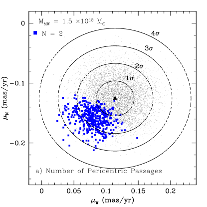
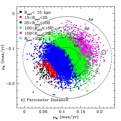
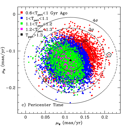
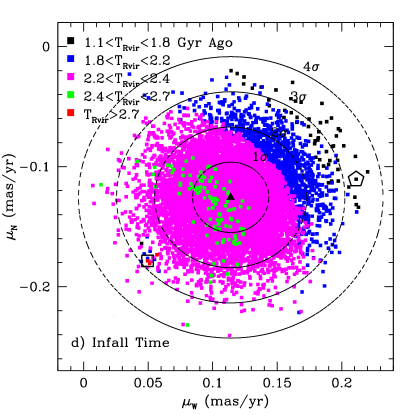
Figure 7.— Similar to Figure 6, but now for the intermediate mass MW model ($M_{\rm vir}=1.5\times 10^{12}$).

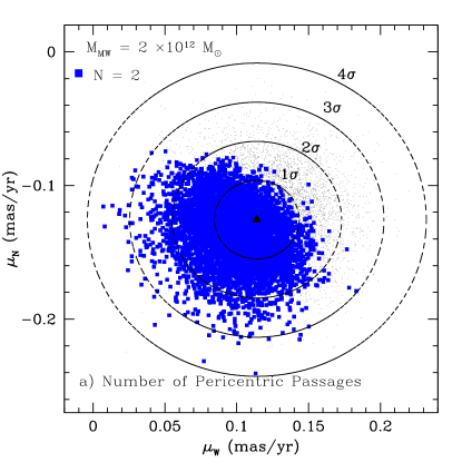
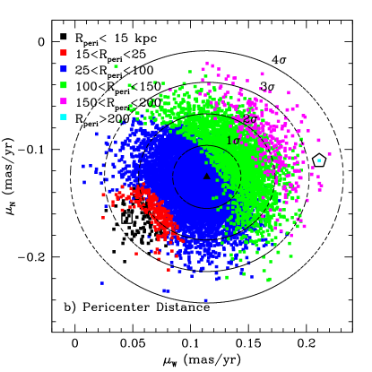
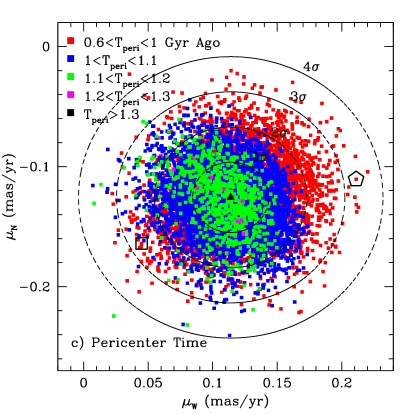
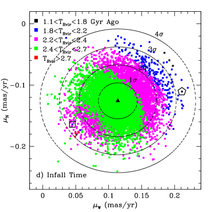
Figure 8.— Similar to Figure 6, but now for the high mass MW model ($M_{\rm vir}=2.0\times 10^{12}$).

Here we present the plausible orbital histories of Leo I following the methodology outlined above. To propagate the observed errors, we randomly sampled 10,000 combinations of the west and north components of the observed Leo I proper motion within the error space provided in Section 2.3. For each of these combinations, the 3D velocity was derived and the orbit of Leo I was followed backward in time for a Hubble time in each of our three MW models. The analysis presented in this section only considers the influence of the MW’s gravitational field on the orbit of Leo I, as described in equation (11).

We seek to define Leo I’s interaction history with the MW by constraining the time and distance of Leo I’s recent pericentric approach to our MW ($r_{\rm peri}$, $t_{\rm peri}$), the number of such encounters it might have had in the past ($N_{\rm peri}$) and the time of infall to our system ($t_{\rm infall}$). We define infall time as the time at which Leo I last crossed the virial radius of the MW. The allowed range in pericenter distance will inform us about the maximal tidal influence the MW may have exerted over Leo I, which may have caused its transformation into a dSph or triggered enhanced star formation activities. The pericenter distance also informs us about the importance of ram pressure stripping by the MW’s gaseous halo in removing gas from this system (e.g., Grcevich & Putman, 2009); the deeper that Leo I travels into the MW’s halo, the higher the background gas density and the more likely gas gets stripped. The infall time is similarly relevant; the longer ago that Leo I was accreted, the longer the time scale for ram pressure stripping to operate. Ultimately, the number of previous pericentric passages will tell us whether Leo I is in fact a recent interloper in our system. These properties can be further used to constrain the halo mass of our own MW statistically by identifying analogs of the Leo I satellite (in terms of mass and orbital properties) about MW-type hosts in large-scale cosmological simulations (see Paper II).

Table 4Mean Orbital Properties of Leo I

$M_{\rm MW}$		$\langle r_{\rm peri}\rangle$	$\langle t_{\rm peri}\rangle$		$\langle d_{\rm apo}\rangle$	$\langle t_{\rm peri,2}\rangle$	$\langle t_{\rm infall}\rangle$
($\times 10^{12}{M_{\odot}}$)	$\langle N_{\rm peri}\rangle$	(kpc)	(Gyr)	$\langle v_{\rm peri}/v_{\rm esc}\rangle$	(kpc)	(Gyr)	(Gyr)	$\langle v_{\rm infall}/v_{\rm Rvir}\rangle$
1.0	$1.0\pm 0.2$	$100\pm 37$	$1.1\pm 0.1$	$1.04\pm 0.07$	$1177\pm 640$	0$7.7\pm 5.6$	$2.2\pm 0.2$	$1.6\pm 0.2$
1.5	$1.0\pm 0.2$	0$90\pm 35$	$1.1\pm 0.1$	$0.96\pm 0.04$	0$558\pm\phantom{0}61$	$12.6\pm 1.3$	$2.3\pm 0.1$	$1.3\pm 0.2$
2.0	$1.5\pm 0.5$	0$82\pm 33$	$1.0\pm 0.1$	$0.91\pm 0.02$	0$530\pm\phantom{0}55$	$11.0\pm 1.7$	$2.5\pm 0.2$	$1.0\pm 0.1$

Note. — Orbital properties as defined in the text. Standard deviations for the mean values are marked. Apocenter distances are computed only for the cases that have a second pericentric approach.

Figures 6, 7 and  8 show the 4$\sigma$ proper motion error space that is sampled to determine the orbital properties of Leo I in the three different MW mass models. Points are color coded to reflect the range of allowed values for the quantity of interest ($N_{\rm peri}$, $r_{\rm peri}$, $t_{\rm peri}$ and $t_{\rm infall}$). The mean values for these quantities are listed in Table 4. In addition, we also list the mean velocity at pericenter relative to the escape speed at $r_{\rm peri}$, ($v_{\rm peri}$/$v_{\rm esc}$), and the velocity at infall relative to the circular velocity of the MW at the virial radius ($v_{\rm infall}/v_{\rm Rvir}$). In the cases where there is a second pericentric approach some time in the past, we list the time this occurs ($t_{\rm peri,2}$) and the mean apocenter distance ($r_{\rm apo}$). We mark the minimum and maximum $r_{\rm peri}$ allowed within the 4$\sigma$ proper motion error space and the times at which they occur in the second and third panels in each of Figures 6, 7 and 8 by the black open square (min) and pentagon (max).

In all cases, Leo I has recently had a pericentric passage with respect to the MW, and so panels (a) in Figures 6, 7 and 8 only note if a second pericentric approach occurs. As the MW mass increases, the likelihood of a second close passage also increases; however there are no cases where a third pericentric approach occurs. In the lowest MW mass model, there are solutions for a second pericentric passage only outside the 2$\sigma$ error ellipse. However, there are only two such solutions out of our 10,000 realizations, one with a second pericenter time of 13 Gyr and the other with 2 Gyr (which is likely a slingshot scenario where Leo I got too close to the MW center). This reflects the fact that for the low-mass MW model, Leo I is generally on a hyperbolic or near-hyperbolic orbit. Solutions for a second pericenter are readily obtainable within the 1$\sigma$ error ellipse for the higher MW mass models. However, the Monte-Carlo statistics (see Table 4) still favor orbits with only one previous pericenter. Moreover, in those cases with a second pericenter, the time since that pericenter is $\gtrsim 10$ Gyr. Also, the apocenter distances are well beyond the virial radius of the MW for all models ($d_{\rm apo}>500$ kpc). Recall that the MW mass was assumed to be static in time; with an accurate treatment of the mass evolution of the MW it is doubtful that any of these second pericentric passages would still occur. It is thus most likely that Leo I has passed its first infall into the MW. Moreover, if the previous pericentric passage occurred $\gtrsim 10$ Gyr ago, this implies that Leo I would be at large distances from the MW exactly a Hubble time ago, which is an implausible scenario in the view of the timing argument.

The average time of Leo I’s most recent pericentric passage is $\sim$1 Gyr ago for all MW models. This is similar to what was found from the Keplerian calculations. The average pericentric approach ranges from 80–100 kpc, and the average velocity at pericenter ranges from 300–$370\>{\rm km}\,{\rm s}^{-1}$ (Table 4). This distance is somewhat larger, and the velocity somewhat smaller, than found from the Keplerian calculations. This is easy to understand from the fact that a Keplerian model is too concentrated, and therefore overestimates the acceleration as Leo I approaches the MW. The average ratio of pericenter to apocenter distance in the orbit calculations ranges from 0.08–0.15. This is larger than in the Keplerian calculations, in part because those calculations ignore the mass outside of the Leo I distance, and therefore overestimate the apocenter distance.

The tidal radius $r_{\rm t}=r_{\rm peri}[2M_{\rm MW}(r_{\rm peri})/M_{\rm Leo~{}I}]^{-1/3}$ of Leo I, given pericentric distances of 80–100 kpc, is 3–4 kpc for the three MW models. The present optical radius of Leo I is $\sim 1$ kpc (Sohn et al., 2007; Walker et al., 2009). This means that on average, the tidal field of the MW does not appear to be sufficient to tidally truncate Leo I to this radius, implying that Leo I likely has an extended dark matter halo. There is a clear trend in $r_{\rm peri}$ with the proper motion as evidenced in panel (b) of Figures 6, 7 and  8; $r_{\rm peri}$ increases with increasing $\mu_{W}$ and $\mu_{N}$. The minimum pericentric approach determined in the 10,000 Monte-Carlo orbits is $\sim$1–2 kpc. However, a pericentric approach of $<5$ kpc is unlikely, because the tidal radius of Leo I in all MW mass models is less that 0.7 kpc. Leo I is not sufficiently disturbed to have approached this close to the MW. On the other hand, pericentric approaches of 20 kpc yield tidal radii of $\sim$1 kpc. Cases where $15<r_{\rm peri}<25$ kpc are found within the 1.5–2$\sigma$ error ellipse in all MW mass models. So such close approaches are not ruled out by our data. However, they are not so likely given our data, with only 2–3% of the Monte-Carlo calculated orbits yielding $r_{\rm peri}<25$ kpc.

The time of Leo I’s last pericentric passage, $\sim 1$ Gyr ago, corresponds roughly to the time when star formation stopped in Leo I (Caputo et al., 1999; Gallart, 1999; Dolphin, 2002; Smecker-Hane et al., 2010). The pericentric approach is the point in time where Leo I would experience maximal ram pressure stripping, which could lead to quenching. All satellites of the MW within 300 kpc (apart from the Magellanic Clouds) are devoid of gas (Grcevich & Putman, 2009), consistent with this picture. As the MW mass increases, $t_{\rm peri}$ decreases; for the most massive MW model the maximal $t_{\rm peri}$ is 1.3 Gyr and the minimal value is 0.6 Gyr. These values are remarkably consistent regardless of MW mass, when searching the full 4$\sigma$ proper motion error space [panels (c)]. Hence, it is likely that star formation stopped in Leo I owing to ram pressure effects at pericentric approach, implying a quenching time scale of $t_{\rm infall}-t_{\rm peri}\approx 1.3\>{\rm Gyr}$ (see Table 4).

Of course, in general, star formation can cease in galaxies for many other reasons, e.g., exhaustion or blowout of the gas supply. However, if this were the cause of star formation ceasing in Leo I, then there would be no natural explanation for why this would coincide with a pericenter passage. On the other hand, this coincidence could certainly happen by chance, especially since the uncertainties in both the SFH and the orbital analysis are significant.

The average infall time ranges from 2.2–2.5 Gyr with little variation, regardless of MW mass. The infall time is similar to the time scale of the most recent enhanced star formation observed in Leo I (Caputo et al., 1999; Gallart, 1999; Dolphin, 2002; Smecker-Hane et al., 2010), suggesting that this enhanced star formation activity was triggered by either ram pressure compression as Leo I entered a higher gas density environment relative to the Local Group, or as it began to feel gravitational torques exerted by the MW. Note that $t_{\rm infall}$ refers to the most recent time at which Leo I entered the virial radius; there are cases where Leo I has made an earlier pericentric approach about the MW. But, as discussed earlier, such orbits may not be physical or plausible. There are a few cases where Leo I remains within the virial radius of the MW for approximately a Hubble Time [indicated by red squares in panels (d)]. However, such a scenario has low likelihood, since these cases are all 4$\sigma$ outliers that only occur in the high mass MW model.

The ratio between the infall velocity and the circular velocity at the virial radius ($v_{\rm Rvir}$) ranges from 1.0–1.6 (Table 4). For the low mass MW model, the average Leo I infall velocities are higher than expected based on cosmological simulations of structure formation, where subhalos are typically accreted with characteristic orbital velocities of $\sim 1.1v_{\rm Rvir}$ at the virial radius (1$\sigma$ scatter of 25%, Wetzel, 2011). This further disfavors masses $M_{\rm MW,vir}\lesssim 10^{12}{M_{\odot}}$.

Our conclusion that Leo I has most likely passed its first infall into the MW, and our value for $t_{\rm infall}$ are consistent with the results of Rocha et al. (2012) for Leo I. They find that there is a tight correlation between the present day orbital energies of the MW satellites and their infall times as inferred from cosmological simulations. We explore the implications of this for our understanding of Leo I further in Paper II.

3.3.3 Comparison to Previous Orbit Estimates

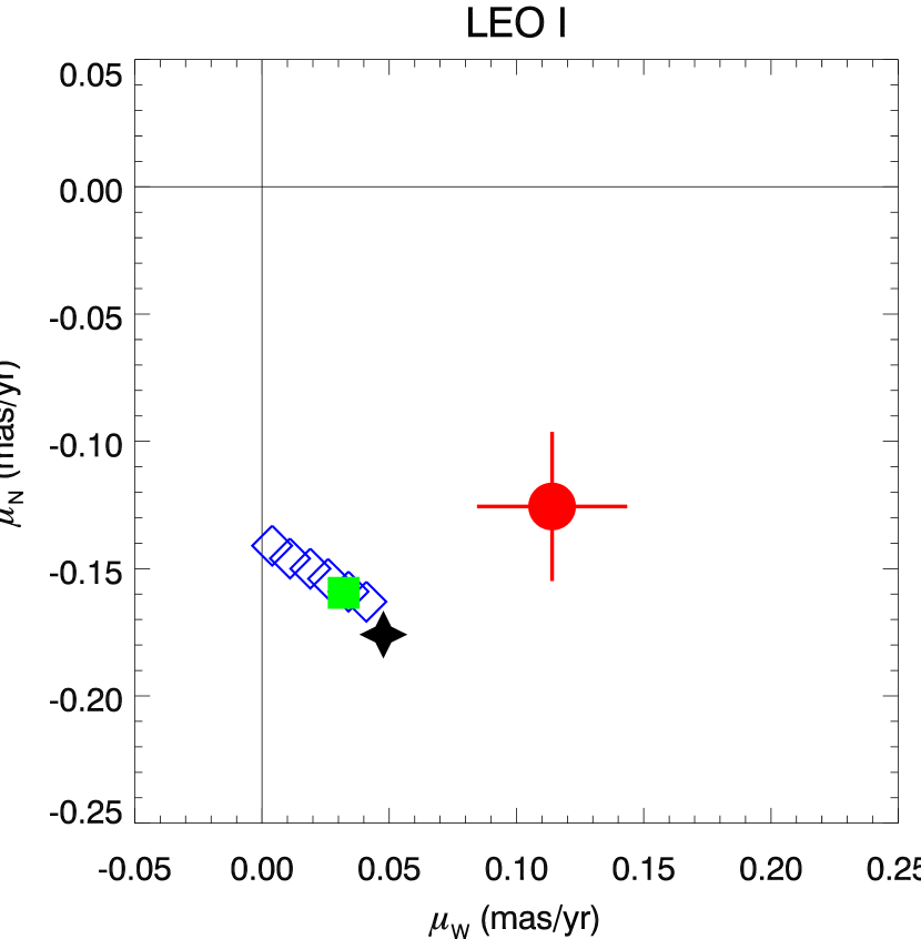
Figure 9.— Comparison between the average Leo I proper motion measured in this study (red data point with error bars) and the proper motions predicted by the models of Sohn et al. (2007) (green closed square) and Mateo et al. (2008) (blue open diamonds). The black cross indicates the proper motion for a radial orbit, i.e., with $V_{\rm tan}=0$, as in Figure 5.

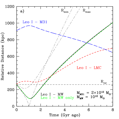
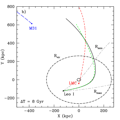
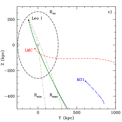
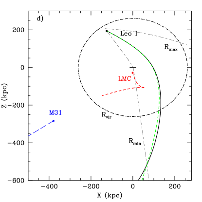
Figure 10.— The mean orbital history of Leo I for the low mass MW model ($M_{\rm vir}=1.0\times 10^{12}{M_{\odot}}$). The mass of M31 is chosen to preserve the total Local Group mass of $3\times 10^{12}{M_{\odot}}$. Panel (a) shows the separation between Leo I and the LMC, MW and M31 as a function of time. In panels (b), (c), and (d), the orbital plane is presented in the Galactocentric $X-Y$, $Y-Z$, and $X-Z$ planes, respectively. The virial radius (R_vir) of the MW is indicated by the dashed horizontal line in panel (a), and the dot-dashed ellipses in the other panels. In panels (b)–(d), the MW location is indicated by the thick black line (circle in the case of the $Y-Z$ plane) centered at (0,0). The current location of each galaxy is indicated by the solid squares. Solid black lines indicate results when Leo I is assumed to be moving with the mean proper motion determined in this study. For comparison, we also plot the orbit of Leo I accounting only for the influence of the MW in dashed green lines. The thin dashed-dotted black lines indicate solutions where the pericenter distance is minimized and maximized [3$\sigma$ outliers; see panel (b) in Figure 6].

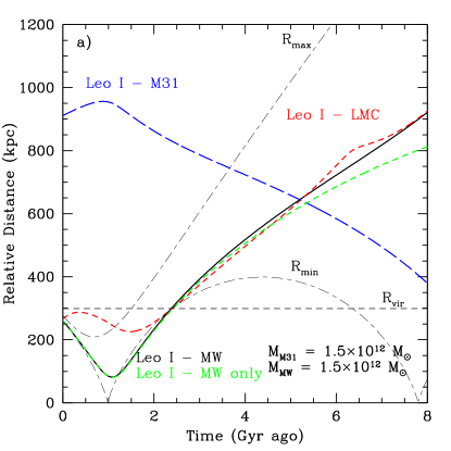
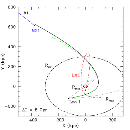
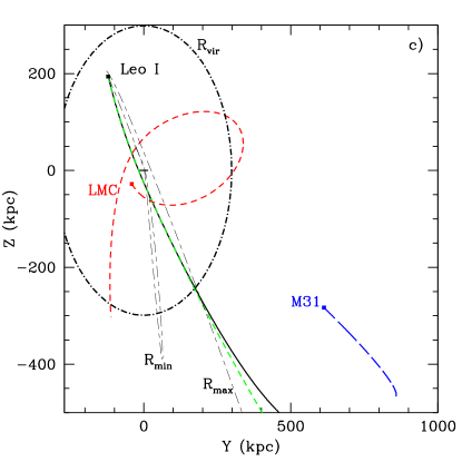
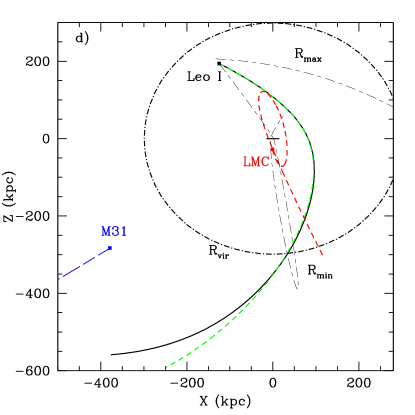
Figure 11.— Similar to Figure 10, but now for the intermediate MW mass model ($M_{\rm vir}=1.5\times 10^{12}{M_{\odot}}$).

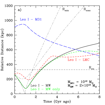
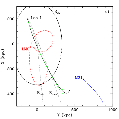
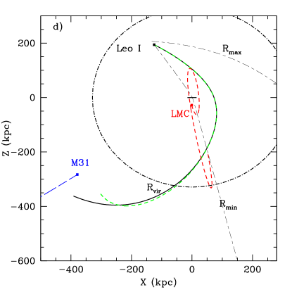
Figure 12.— Same to Figure 10, but now for the high MW mass model ($M_{\rm vir}=2.0\times 10^{12}{M_{\odot}}$).

Sohn et al. (2007) and Mateo et al. (2008) provided estimates of the orbital history of Leo I based on indirect arguments, rather than proper motion measurements. They aimed in particular to explain the photometric and kinematical data of giants stars in Leo I. The proper motions corresponding to the proposed orbits are compared to our new HST measurements in Figure 9. The orbits of Sohn et al. (2007) had a pericentric approach of only $\sim 10$ kpc, so the predicted proper motion is very close to the $V_{\rm tan}=0$ point. Mateo et al. (2008) provided proper motion predictions for a range of assumed Leo I masses (their Table 8). While their predicted perigalactic distances reach out to 30 kpc, their proper motions lie on the opposite side of the $V_{\rm tan}=0$ point compared to our measurements. So our measurements do not confirm the predictions of these studies. More specifically, the previous studies argued for highly eccentric orbits with smaller perigalactic distances than what we find here.

Sohn et al. (2007) focused primarily on trying to reproduce the observed photometric and kinematic features of Leo I by adopting a tidal disruption scenario. The orientation of their model orbits was determined by assuming that the position angle of the Leo I ellipticity and the orientation of the break population are caused by tidal effects and tidal stripping, respectively. They showed that the observed features can be plausibly produced by the tidal effects of the MW. However, the tidal effects may have been overestimated, given that the orbital properties derived here imply that Leo I is on a less eccentric orbit than assumed by Sohn et al. (2007). This discrepancy does not imply though that the tidal scenarios used by Sohn et al. (2007) and Mateo et al. (2008) are necessarily wrong. It may just be that some of the specific assumptions in their models were oversimplified. For example, if Sohn et al. (2007) had not modeled the progenitor satellite as a spherical Plummer profile, the best-fit orbits may well have been more consistent with the observed proper motion. New $N$-body models based on the observed proper motion should be able to further improve our understanding of the tidal disruption features observed in Leo I. However, such models are beyond the scope of the present paper.

3.3.4 Leo I Orbital Plane

Here we compute the orbital history of Leo I, relative to the other major players in the Local Group, namely the MW, the LMC, and M31. We aim to define Leo I’s orbital plane and compare it to that of the LMC, and to determine whether Leo I was ever close enough to M31 for it to have exerted any dynamical influence in Leo I’s history.

In Figures 10, 11, and 12 we plot the orbit of Leo I using the mean proper motions determined in this study, including the influence of the MW, LMC, and M31 (solid black line). For comparison, we also plot the orbit of Leo I accounting only for the influence of the MW (dashed green line). Orbits corresponding to proper motions that are $\pm$3$\sigma$ from the mean (identified as having min/max pericenter distances to the MW from panels (b) in Figures 6, 7, and 8) are indicated by the thin dash-dotted black lines (Rmin and Rmax) in all panels.

Panels (a) illustrate the separation of Leo I from the other galaxies and Panels (b), (c), and (d) respectively show the orbits of the galaxies in the $X$-$Y$, $Y$-$Z$, and $X$-$Z$ Galactocentric planes. As the MW mass increases, Leo I’s past orbit becomes less eccentric and increasingly directed towards M31. It is clear that Leo I does not get closer than 400 kpc from M31 in any model over the past 8 Gyr and neither the presence of M31 nor the LMC have an impact on the infall time or pericenter properties. However, M31 may play a role at early times in the higher MW mass models; the orbits are more energetic, reaching larger distances than if the gravity of the MW were considered alone. We note that we have not accounted for the mass evolution of the MW or M31, which will diminish the role that M31 plays at early times. But, this analysis does suggest that accounting for the local overdensity (i.e. that there are two roughly equal mass galaxies in our Local Group) may be a relevant parameter in understanding the origin of the angular momentum of high speed satellites. In this study, such considerations are only relevant for the higher mass MW models; in the lowest mass MW model, Leo I is too far from M31 at all times for torques to be relevant. Our conclusions regarding the hyperbolic nature of Leo I’s orbit in low-mass MW models is thus robust to the influence of M31 and can be compared statistically to satellite orbits found in cosmological simulations of isolated MW analogs (see Paper II).

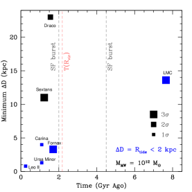
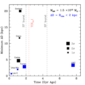
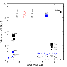
Figure 13.— The minimum separation to Leo I that is allowed within the proper motion error space of each satellite is plotted as a function of time for each MW mass model. Cases where the separation is sufficiently small so as to tidally truncate Leo I to within at least 2 kpc are marked in blue. Given the low mass ratios, such separations will also allow Leo I to influence that satellite in turn, except for the LMC. Black dashed lines indicate known epochs of enhanced star formation activity in Leo I, as discussed in the text. The red dashed line indicates its infall time within the virial radius of the MW. The size of each point indicates the distance of the corresponding Leo I proper motion from the mean observed proper motion, as described in the legend; smaller points are more likely. Although events were found within 1$\sigma$ for some satellites, they typically represent only $\lesssim 4$% of the Monte-Carlo drawings. This is shown explicitly in Figure 14 for the satellites that have the closest encounters, Ursa Minor and Leo II, to illustrate the low probability of such encounters. We note that Sculptor never gets closer to Leo I than its current separation and is thus omitted from the plot.

The minimum pericentric passage orbits appear to be slingshot orbits, approaching near the MW center, gaining energy and traveling to larger distances. However, as discussed in Section 3.3.2, such orbits are likely unphysical because Leo I is not sufficiently disturbed to have traveled this close to the MW. Since the orbit of Leo I is still bound to the MW in the vast majority of models, we do not need a small pericenter, slingshot orbit to explain the orbital properties of Leo I.

Panels (b), (c), and (d) respectively show the orbits of the galaxies in the $X$-$Y$, $Y$-$Z$, and $X$-$Z$ Galactocentric planes. The orbital angular momentum of Leo I is not coincident with that of the LMC. This is most clearly illustrated when looking at the orbital history in the $X$-$Z$ Galactocentric plane, especially in the higher-mass MW models. The LMC is moving in a clockwise direction in this plane whereas Leo I is moving counterclockwise.

3.3.5 Interactions with other Satellites

We have so far established that Leo I is likely on its first orbit around the MW and that its most recent pericentric approach was likely at a separation of 80–100 kpc, too large for the MW to have exerted significant tidal torques. Yet, Leo I shows signs of a past interaction. Sohn et al. (2007) found an excess of red giant stars along the major axis of Leo I’s main body relative to a symmetric King profile. In addition to this spatial configuration, Leo I red giant stars have an asymmetric radial velocity distribution at large radii (cf., see also Mateo et al., 2008). If the MW is not the culprit for the distorted structure and kinematics of Leo I, then what is?

Here we consider the orbital history of not only Leo I, but also of the other satellite galaxies of the MW simultaneously. We randomly sampled 10,000 combinations of the observed west and north components of the proper motion within the 4$\sigma$ error space for Leo I and for each satellite. The proper motions, distances, and radial velocities were taken from various sources as listed in Table 3. As for Leo I, we took the distance for each satellite to be the error-weighted average of TRGB measurements in the last decade. The proper motions and radial velocities were adopted from the most recent measurements available in the literature. We computed the orbits of all satellites backwards in time for 10 Gyr using each of our three MW models, and using the mass model for each satellite outlined in Table 3. Our goal is to determine the closest separation that Leo I may have reached to any of these other satellites within the error space and to assess whether such separations are sufficient to exert torques on Leo I and induce star formation or to significantly modify Leo I’s orbit.

Given the small masses of these satellites, their dynamical influence is minimal unless the separation between them is small. Overall, satellite separations as low as 3–4 kpc are required before one can significantly influence the other, i.e. such that the tidal radius of the satellite is less than 2 kpc. Because the LMC is much more massive than the other satellites, a larger separation of at least 20 kpc will allow it to distort Leo I to within 2 kpc. Of course, Leo I is much too small to strongly affect the LMC.

Figure 13 indicates the minimum separation between each satellite and Leo I as a function of time for each respective MW mass model. Satellites that reach separations within their 4$\sigma$ error space small enough to influence Leo I within a radius of 2 kpc (and vice versa) are highlighted in blue. The size of the point reflects the probability of that encounter, based on the sigma deviation of the required Leo I proper motion from the mean. Vertical dashed lines indicate relevant events in the history of Leo I, such as epochs of star formation and the epoch of infall into the MW.

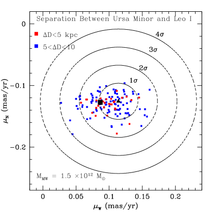
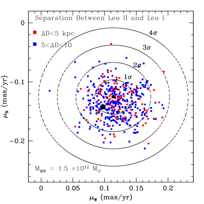
Figure 14.— Orbits, out of 10,000 randomly selected points from the 4$\sigma$ error space of the Leo I proper motions, that produce a passage of Ursa Minor (left panel) or Leo II (right panel) within 10 kpc of Leo I. Orbits are color coded based on the minimum separation, as calculated for the intermediate MW mass model ($M_{\rm vir}=1.5\times 10^{12}{M_{\odot}}$). Separations less than 3 kpc are readily found within the 1$\sigma$ error ellipse, indicating that such past encounters are possible. For Ursa Minor, there are 62 blue points and 19 red points that fall within the 1$\sigma$ region (the innermost circle), and for Leo II, there are 171 blues points and 57 red points within the 1$\sigma$ region.

There are no obvious satellite encounters found that can explain the enhanced star formation activities at $\sim 2$ and $\sim 4.5$ Gyr ago. It appears much more likely that the enhancement of star formation that took place $\sim 2$ Gyr ago is related to the epoch of accretion by the MW. While there are some parameter combinations that allow for close encounters between Leo I and Fornax, Carina and the LMC, these are likely random events as there are only ever 2, or 3 points within the 10,000 orbit search that yield such encounters. Also, Sculptor never gets close to Leo I than it is today, and is thus omitted from the plot. Among the MW satellites we consider, there is a higher probability – though still relatively small – of an encounter with Ursa Minor and Leo II for all MW models. Specifically, 1.3% and 4.5% of the Monte-Carlo calculated orbits yield passages within 10 kpc for Ursa Minor and Leo II, respectively. These encounters are expected to have occurred within the past 1 Gyr, well after star formation has ceased in all of these galaxies (Carrera et al., 2002; Koch et al., 2007; Kirby et al., 2011). The encounter is thus unlikely to have signatures in the star formation histories of these galaxies, as they should already have been devoid of gas at that point. However, there may be kinematical signatures instead. In particular the distortions in Leo I noted by Sohn et al. (2007) could be explained by collisions with Ursa Minor or Leo II, rather than interactions with the MW. Ursa Minor is also known to be kinematically disturbed (Kleyna et al., 1998; Wilkinson et al., 2004). It has an inner bar that has been suggested to be tidally induced (Łokas et al., 2012) and has an extended stellar halo (Palma et al., 2003). To date, however, no sign of tidal disturbance is found for Leo II.

To illustrate the non-negligible probability of such encounters, we focus in Figure 14 on orbit calculations for the intermediate mass MW mass model ($M_{\rm vir}=1.5\times 10^{12}{M_{\odot}}$). We plot from the 10,000 randomly sampled points within the 4$\sigma$ proper motion error space, those points that produce a passage of Ursa Minor (left panel) or Leo II (right panel) within 10 kpc of Leo I. There are several orbital solutions within 1$\sigma$ with such small separations to Leo I. Since the error space of the Leo II and Ursa Minor proper motions were also searched, we note here that solutions are also found within 1$\sigma$ of their respective means. So close encounters between these galaxies and Leo I are not ruled out by the data, although the probability of such encounters is low. The encounter time for Ursa Minor occurs within a range of 0.8-1.1 Gyr ago, while the encounter time for Leo II is relatively recent, with a range of 0.15–0.3 Gyr ago.

To determine whether the presence of the satellites of the MW can modify the orbit of Leo I, we repeated the analysis of Section 3.3.2, but now also accounting for the tidal torques exerted by the other satellites. We followed the method outlined above to test the proper motion error space for each satellite in Monte-Carlo sense. This showed that any multi-body tidal effects by the other MW satellites are insufficient to modify the average orbital properties listed in Table 4. In particular, the average velocity and time at infall are unaffected by the presence of the other MW satellites. We find that the Leo I orbit is significantly affected by the presence of the other satellites in only $0.1$–$0.2$% of Monte-Carlo orbits. So Leo I’s high velocity is probably not a product of multi-body tidal torques. This makes it important to address whether such a high velocity can arise naturally in $\Lambda$CDM galaxy assembly scenarios without assistance from multi-body interactions. We explore this topic in detail in Paper II.

4. Conclusions

We have presented the first absolute proper motion measurement of Leo I, based on HST ACS/WFC images taken in two different epochs separated by $\sim 5$ years. We used the method of Sohn et al. (2012) to measure the average bulk motion of Leo I stars with respect to stationary distant galaxies in the background. We detect motion of Leo I at $4\sigma$ confidence, and find its proper motion to be ($\mu_{W},\mu_{N}$) = ($0.1140\pm 0.0295,-0.1256\pm 0.0293$) mas yr^-1. The uncertainties are smaller than those obtained in previous HST studies of other MW satellites that used a background quasar as stationary reference. To derive the velocity of Leo I with respect to the MW, we combined the proper motion with the known line-of-sight velocity and corrected for the solar reflex motion. The resulting Galactocentric radial and tangential velocities are $V_{\rm rad}=167.9\pm 2.8$ and $V_{\rm tan}=101.0\pm 34.4\>{\rm km}\,{\rm s}^{-1}$, respectively. Hence, Leo I has a significant transverse velocity, but it is less than the radial velocity.

Combined with its current position, the new knowledge of the three-dimensional velocity of Leo I has allowed us to study its orbital history in detail. To evaluate the past orbit we employed a range of mass models of increasing complexity. Starting from Keplerian models for the MW, we progressed first to cosmologically motivated MW models of $M_{vir}=1.0\times 10^{12},1.5\times 10^{12}$, and $2.0\times 10^{12}{M_{\odot}}$, and then to models in which other MW satellites and Local Group galaxies are included as well. In each of these models we solved the equations of motion to follow the Leo I velocity and position backward in time. We used a Monte-Carlo analysis to explore the impact of the observational measurement uncertainties.

Allowing for both observational uncertainties and uncertainties in the MW mass model (Table 4, with a flat prior in mass), we find that Leo I’s most recent perigalactic passage was $1.05\pm 0.09$ Gyr ago at a Galactocentric distance of $91\pm 36$ kpc. The ratio of the orbital pericenter to apocenter distance is $0.17\pm 0.07$, so the orbit extends well outside of the MW’s virial radius. Leo I entered the virial radius $2.33\pm 0.21$ Gyr ago. This was most likely Leo I’s first infall into the MW. A previous pericenter, which would have occurred almost a Hubble time ago, becomes slightly plausible only in the highest-mass MW models.

Stellar population studies of Leo I have inferred that it experienced an enhancement in star formation $\sim 2$ Gyr ago. This may have been the result of Leo I entering the virial radius of the MW for the first time, leading to gas compression through ram pressure or MW tidal torques. Stellar population studies have also shown that star formation in Leo I was quenched $\sim 1$ Gyr ago. This may have been due to the pericentric approach of Leo I with respect to the MW, at which point ram pressure stripping of gas was maximal.

A previously inferred enhanced star formation activity in Leo I that occurred $\sim 4.5$ Gyr ago is not obviously associated with any orbital time scale, or interaction with any other galaxy. The orbital plane of Leo I is not coincident spatially or in rotational sense to that of the LMC. The separation between M31 and Leo I remains large at early times, but it may have been possible that M31 applied sufficient torques at early times to have modified Leo I’s orbit. Leo I may have closely approached (within $\sim 10$ kpc) other MW satellites, but only in the last Gyr, and with probabilities of at most a few percent. The probabilities are highest for past encounters with Ursa Minor or Leo II, which may have left marks in the kinematical properties of Leo I or these other galaxies.

Given the observed velocity of Leo I and prior constraints on the MW virial mass, Leo I is most likely bound to the MW. However, this is not true in MW models with masses $M_{vir}\lesssim 10^{12}$, at the low end of the allowed range. Leo I has just passed pericenter, probably from its first infall into the MW. So its kinematics are probably not virialized. So even though Leo I is probably bound, it is not necessarily appropriate to include it in equilibrium models of the MW satellite population, such as those that are often used to estimate the MW virial mass (e.g., Watkins et al., 2010).

The velocity of Leo I can also be used to estimate the MW mass through the timing argument. Previous studies of this kind have used the assumption of a radial orbit, but with a statistical correction for any possible transverse velocity (e.g., Li & White, 2008). Now that the transverse velocity has actually been measured, it is possible to solve the complete timing equations for a non-radial orbit. This yields $M_{\rm{MW,vir}}=3.15_{-1.36}^{+1.58}\times 10^{12}{M_{\odot}}$, with the large uncertainty dominated by cosmic scatter. This is higher than, but not inconsistent with, the range of MW mass estimates obtained from other methods.

This is the first paper in a series of two. In Paper II, we compare the new observations to the properties of Leo I subhalo analogs extracted from state-of-the-art cosmological simulations. We show there that Leo I is most likely bound to the MW, since unbound subhalos are extremely rare at the present epoch. We also show there that the observed kinematics of Leo I are more consistent with high-mass than with low-mass MW models. Both these conclusions are consistent with what we have inferred in the present paper through different arguments.

In this paper and in Sohn et al. (2012), we have used our new methodologies to successfully measure with HST the absolute proper motions of Leo I and M31, respectively. The new measurements have allowed us to derive new constraints on the past and future orbital evolution of the target galaxies, and on the mass of the Local Group’s dominant galaxies, the MW and M31. Motivated by these results, we are continuing to apply our proper motion measurement techniques to a range of other topics in Local Group galaxy research. For example, our group has ongoing HST observing programs to measure the proper motions of: (1) dwarf galaxies near the edge of the Local Group (GO-12273, PI: R. P. van der Marel); (2) stars at different locations in the Sagittarius Stream (GO-12564, PI: R. P. van der Marel); and (3) the dwarf galaxy Leo T, which is likely a galaxy falling into the MW for the first time (GO-12914, PI: T. Do). We expect that the results from these ongoing programs will further constrain the dark matter distribution in the Local Group and its dominant galaxies.

References

- Anderson & King (2006) Anderson J., & King, I. R. 2006, ACS/ISR 2006-01, PSFs, Photometry, and Astrometry for the ACS/WFC (Baltimore: STScI) (AK06)
- Anderson & Bedin (2010) Anderson, J. & Bedin, L. R. 2010, PASP, 122, 1035
- Armandroff et al. (1995) Armandroff, T. E., Olszewski, E. W., & Pryor, C. 1995, AJ, 110, 2131
- Bellazzini et al. (2002) Bellazzini, M., Ferraro, F. R., Origlia, L., et al. 2002, AJ, 124, 3222
- Bellazzini et al. (2004) Bellazzini, M., Gennari, N., Ferraro, F. R., & Sollima, A. 2004, MNRAS, 354, 708
- Bellazzini et al. (2005) Bellazzini, M., Gennari, N., & Ferraro, F. R. 2005, MNRAS, 360, 185
- Benson (2005) Benson, A. J. 2005, MNRAS, 358, 551
- Bersier (2000) Bersier, D. 2000, ApJ, 543, L23
- Bertin & Arnouts (1996) Bertin, E., & Arnouts, S. 1996, A&AS, 117, 393
- Besla et al. (2007) Besla, G., Kallivayalil, N., Hernquist, L., et al. 2007, ApJ, 668, 949
- Besla et al. (2012) Besla, G., Kallivayalil, N., Hernquist, L., et al. 2012, MNRAS, 421, 2109
- Boylan-Kolchin et al. (2012) Boylan-Kolchin, M., Bullock, J. S., & Kaplinghat, M. 2012, MNRAS, 422, 1203
- Boylan-Kolchin et al. (2013) Boylan-Kolchin, M., Bullock, J. S., Sohn, S. T., Besla, G., & van der Marel, R. P. 2013, ApJ, in press (Paper II)
- Bovy et al. (2012) Bovy, K., Allende Prieto, C., Beers, T. C., et al. 2012, ApJ, 759, 131
- Byrd et al. (1994) Byrd, G., Valtonen, M., McCall, M., & Innanen, K. 1994, AJ, 107, 2055
- Caputo et al. (1999) Caputo, F., Cassisi, S., Castellani, M., Marconi, G., & Santolamazza, P. 1999, ApJ, 117, 2199
- Carrera et al. (2002) Carrera, R, Aparicio, A., Martínez-Delgado, D., & Alonso-García, J. 2002, AJ, 123, 3199
- Courteau & van den Bergh (1999) Courteau, S., & van der Bergh, S. 1999, AJ, 118, 337
- Deason et al. (2011) Deason, A. J., McCarthy, I. G., Font, A.S., et al. 2011, MNRAS, 415, 2607
- Dehnen & Binney (1998) Dehnen, W., & Binney, J. J. 1998, MNRAS, 298, 387
- D’Onghia & Lake (2008) D’Onghia, E. & Lake, G. 2008, ApJ, 686, 61
- Dolphin (2002) Dolphin, A. E. 2002, MNRAS, 332, 91
- Efron & Tibshirani (1993) Efron, B., & Tibshirani, R. 1993, An Introduction to the Bootstrap (New York: Chapman & Hall/CRC)
- Fakhouri et al. (2010) Fakhouri, O., Ma, C. -P., & Boylan-Kolchin, M. 2010, MNRAS, 406, 2267
- Freedman & Madore (1990) Freedman, W. L., & Madore, B. F. 1990, ApJ, 365, 186
- Freedman et al. (2001) Freedman, W. L., Madore, B. F., Gibson, B. K., et al. 2001, ApJ, 553, 47
- Gallart (1999) Gallart, C., Freedman, W. L., Aparicio, A., Bertelli, G., & Chiosi, C. 1999, AJ, 118, 2245
- Gnedin et al. (2004) Gnedin, O., Kravtsov, A. V., Klypin, A. & Nagai, D. 2004, ApJ, 616, 16
- Grcevich & Putman (2009) Grcevich. J & Putman, M. E. 2009, ApJ, 696, 385
- Grillmair (2009) Grillmair, C. J. 2009, ApJ, 693, 1118
- Gullieuszik et al. (2007) Gullieuszik, M., Held, E. V., Rizzi, L., et al. 2007, A&A, 467, 1025
- Gullieuszik et al. (2008) Gullieuszik, M., Held, E. V., Rizzi, L., et al. 2008, MNRAS, 388, 1185
- Hargreaves et al. (1994) Hargreaves, J. C., Gilmore, G., Irwin, M. J., & Carter, D. 1994, MNRAS, 269, 957
- Held et al. (2010) Held, E. V., Gullieuszik, M., Rizzi, L., et al. 2010, MNRAS, 404, 1475
- Hernquist (1990) Hernquist, L. 1990, ApJ, 356, 359
- Kahn & Woltjer (1959) Kahn, F. D., & Woltjer, L. 1959, ApJ, 130, 705
- Kallivayalil et al. (2006a) Kallivayalil N., van der Marel, R. P., Alcock, C., et al. 2006a, ApJ, 638, 772
- Kallivayalil et al. (2006b) Kallivayalil N., van der Marel, R. P., & Alcock, C., 2006b, ApJ, 652, 1213
- Kallivayalil et al. (2013) Kallivayalil N., van der Marel, R. P., Besla, G., Anderson, J., & Alcock, C. 2013, ApJ, 764, 161
- Kirby et al. (2011) Kirby, E., Cohen, J. G., Smith, G. H., et al. 2011, ApJ, 727, 79
- Klypin et al. (2011) Klypin, A. A., Trujillo-Gomez, S., & Primack, J. 2011, ApJ, 740, 102
- Kleyna et al. (1998) Kleyna, J. T., Geller, M. J., Kenyon, S. J., Kurtz, M. J. & Thorstensen, J. R. 1998, AJ, 115, 2359
- Koch et al. (2007) Koch A., Kleyna, J. T., Wilkinson, M. I., et al. 2006, AJ, 134, 566
- Kochanek (1996) Kochanek, C. S. 1996, ApJ, 457, 228
- Kulessa & Lynden-Bell (1992) Kulessa, A. S., & Lynden-Bell, D. 1992, MNRAS, 255, 105
- Kunkel & Demers (1976) Kunkel, W. E., & Demers, S. 1976, in Royal Greenwich Observatory Bulletin, Vol. 182, The Galaxy and the Local Group, ed. R. J. Dickens, J. E. Perry, F. G. Smith, & I. R. King (Herstmonceux: The Observatory), 241
- Lee et al. (2003) Lee, M. G., Park, H. S., Park, J. -H., et al. 2003, AJ, 126, 2840
- Lépine et al. (2011) Lépine, S., Koch, A., Rich, R. M., & Kuijken, K. 2011, ApJ, 741, L100
- Li & White (2008) Li, Y. -S., & White, S. D. M. 2008, MNRAS, 384, 1459
- Łokas et al. (2012) Łokas, E. L., Majewski, S. R., Kazantzidis, S., et al. 2012, ApJ, 751, 61
- Lynden-Bell (1976) Lynden-Bell, D. 1976, MNRAS, 174, 695
- Mahmud & Anderson (2008) Mahmud N., & Anderson, J. 2008, PASP, 120, 907
- Majewski et al. (2003) Majewski, S. R., Skrutskie, M. F., Weinberg, M. D., & Ostheimer, J. C. 2003, ApJ, 599, 1082
- Mateo et al. (1993) Mateo, M., Olszewski, E. W., Pryor, C., Welch, D. L., & Fischer, P. 1993, AJ, 105, 510
- Mateo et al. (1998) Mateo, M., Olszewski, E. W., Vogt, S. S., & Keane, M. J. 1998, AJ, 116, 2315
- Mateo et al. (2008) Mateo, M., Olszewski, E. W., & Walker, M. G. 2008, ApJ, 675, 201
- McMillan (2011) McMillan, P. J. 2011, MNRAS, 414, 2446
- Méndez et al. (2002) Méndez, B., Davis, M., Moustakas, J., et al. 2002, AJ, 124, 213
- Metz et al. (2009) Metz, M., Kroupa, P., Theis, C., Hensler, G., & Jerjen, H. 2009, ApJ, 697, 269
- Miyamoto & Nagai (1975) Miyamoto, M., & Nagai, R. 1975, PASJ, 27, 533
- Navarro et al. (1997) Navarro, J. F., Frenk, C.S., & White, S. D. M. 1997, ApJ, 490, 493
- Palma et al. (2003) Palma, C., Majewski, S. R., Siegel, M. H., et al. 2003, AJ, 125, 1352
- Piatek et al. (2005) Piatek, S., Pryor, C., Bristow, P., et al. 2005, AJ, 130, 95
- Piatek et al. (2006) Piatek, S., Pryor, C., Bristow, P., et al. 2007, AJ, 131, 1445
- Piatek et al. (2007) Piatek, S., Pryor, C., Bristow, P., et al. 2007, AJ, 133, 818
- Piatek et al. (2008) Piatek, S., Pryor, C., & Olszewski, E. W. 2008, AJ, 135, 1024
- Piatek et al. (2003) Piatek, S., Pryor, C., Olszewski, E. W., et al. 2003, AJ, 126, 2346
- Pietrzynski et al. (2008) Pietrzynski, G., Gieren, W., Szewczyk, O., et al. 2008, AJ, 135, 1993
- Pietrzynski et al. (2009) Pietrzynski, G., Górski, M., Gieren, W., et al. 2009, AJ, 138, 459
- Queloz et al. (1995) Queloz, D., Dubath, P., & Pasquini, L. 1995, A&A, 300, 31
- Rizzi et al. (2007a) Rizzi, L., Held, E. V., Saviane, I., Tully, R. B., & Gullieuszik, M. 2007a, MNRAS, 380, 1255
- Rizzi et al. (2007b) Rizzi, L., Tully, R. B., Makarov, D., et al. 2007b, ApJ, 661, 815
- Rocha et al. (2012) Rocha, M., Peter, A. H. G., & Bullock, J. 2012, MNRAS, 425, 231
- Sales et al. (2007) Sales, L. V., Navarro, J. F., Abadi, M. G., & Steinmetz, M. 2007, MNRAS, 379, 1475
- Sales et al. (2011) Sales, L. V., Navarro, J. F., Cooper, A. P., et al. 2011, MNRAS, 418, 648
- Saviane et al. (2000) Saviane, I., Held, E. V., & Bertelli, G. 2000, A&A, 355, 56
- Scholz & Irwin (1994) Scholz, R. -D., & Irwin, M. J. 1994, in MacGillivray H. T., Thomson E. B., Lasker B. M., Reid I. N., Malin D. F., West R. M., Lorenz H., eds, Proc. IAU Symp. 161, Astronomy from Wide Field Imaging. Kluwer, Dordrecht, p. 535
- Schönrich et al. (2010) Schönrich, R., Binney, J., & Dehnen, W. 2010, MNRAS, 403, 1829
-
Smecker-Hane et al. (2010)
Smecker-Hane, T. A., Marsteller, B., Cole, A., Gallagher, J. S., & Bullock, J. S.
2010, in Contribution Summaries of the STScI 2010 May Symposium: Stellar Populations
in the Cosmological Context, 90,
http://www.stsci.edu/institute/conference/spring2010/
MaySymp2010PunchLine.pdf - Sohn et al. (2007) Sohn, S. T., Majewski, S. R., Muñoz, R. R., et al. 2007, ApJ, 663, 960
- Sohn et al. (2010) Sohn, S. T., Anderson, J., & van der Marel, R. P. 2010, in 2010 Space Telescope Science Institute Calibration Workshop - Hubble after SM4. Preparing JWST, ed. S. Deustua, & C. Oliveira (Baltimore, MD: STScI), p. 35
- Sohn et al. (2012) Sohn, S. T., Anderson, J., & van der Marel, R. P. 2012, ApJ, 753, 7
- van der Marel et al. (2002) van der Marel, R. P., Alves, D. R., Hardy, E., & Suntzeff, N. B. 2002, AJ, 124, 2639
- van der Marel & Guhathakurta (2008) van der Marel, R. P., & Guhathakurta, P. 2008, ApJ, 678, 187
- van der Marel et al. (2012a) van der Marel, R. P., Fardal, M., Besla, G., et al. 2012a, ApJ, 753, 8
- van der Marel et al. (2012b) van der Marel, R. P., Besla, G., Cox, T. J., Sohn, S. T., & Anderson, J. 2012b, ApJ, 753, 9
- Walker et al. (2006) Walker, M. G., Mateo, M., Olszewski, E. W., et al. 2006, AJ, 131, 2114
- Walker et al. (2008) Walker, M. G., Mateo, M., & Olszewski, E. W. 2008, ApJ, 688, L75
- Walker et al. (2009) Walker, M. G., Mateo, M., & Olszewski, E. W. 2009, AJ, 137, 3100
- Wang et al. (2013) Wang, J., Frenk, C. S., & Cooper, A. P. 2013, MNRAS, 429, 1502
- Watkins et al. (2010) Watkins, L. L., Evans, N. W., & An, J. H. 2010, MNRAS, 406, 264
- Wetzel (2011) Wetzel, A. R. 2011, MNRAS, 412, 49
- Wilkinson & Evans (1999) Wilkinson, M. I., & Evans, N. W. 1999, MNRAS, 310, 645
- Wilkinson et al. (2004) Wilkinson, M. I., Kleyna, J. T., Evans, N. W., et al. 2004, ApJ, 611, 21
- Wolf et al. (2010) Wolf, J., Martinez, G. D., Bullock, J. S., et al. 2010, MNRAS, 406, 1220
- Zaritsky et al. (1989) Zaritsky, D., Olszewski, E. W., Schommer, R. A., Peterson, R. C., & Aaronson, M. 1989, ApJ, 345, 759