Sudakov Resummation in Small-$x$ Saturation Formalism

Abstract

Through an explicit calculation of massive scalar particle (e.g., Higgs boson) production in high energy $pA$ collisions up to one-loop order, we demonstrate that the Sudakov-type logarithms in hard processes in small-$x$ saturation formalism can be systematically separated from the typical small-$x$ logarithms. The generic feature of the Sudakov logarithms and all order resummation is derived. We further comment on the phenomenological implications and extension to other hard processes in the small-$x$ calculations.

1. Introduction. An important application of the perturbative quantum chromodynamics (QCD) is the resummation. In high energy hadronic processes involving large separate scales, resummation is not only necessary to make reliable predictions, but also crucial to extract the fundamental properties of the strong interaction theory, such as the strong coupling constant. In practice, the resummation formalism has been applied to a wide range of physics processes. One of the examples is the resummation of the Sudakov-type double logarithms Sudakov:1954sw ; Collins:1984kg . The double logarithms appear in, for example, the transverse momentum spectrum of a hard process, where each order of perturbative correction is accompanied by a large double logarithmic term of $\ln^{2}(Q^{2}/k_{\perp}^{2})$ with $Q$ the large momentum scale and $k_{\perp}$ the transverse momentum. In low transverse momentum region where most of the production events sit, the QCD resummation has to be performed. This resummation is often referred as the transverse momentum resummation.

Meanwhile, there is also small-$x$ resummation which is equally important, in particular, in the area of the large hadron collider (LHC). Small-$x$ resummation is governed by the BFKL evolution Balitsky:1978ic . Because of high gluon density in nucleon/nucleus, the non-linear term in the evolution plays a very important role at small-$x$ Gribov:1984tu ; Mueller:1985wy ; McLerran:1993ni , which leads to the BK-JIMWLK evolution Balitsky:1995ub ; JalilianMarian:1997jx ; Iancu:2000hn . As a result, the gluon saturation with a characteristic scale $Q_{s}^{2}$ becomes inevitable at small-$x$. Seeking for the signal of the gluon saturation phenomena and studying the associated dynamics has been one of the most important motives for the high energy nucleon-nucleus experiments at RHIC and the LHC, and for the planed electron-ion colliders. Great efforts have been made from both experiment and theory sides eic . Among them, the hard processes involving a large momentum scale have been emphasized recently as important probes for the saturation phenomena Dominguez:2010xd . This is because these hard processes can directly measure the transverse momentum dependence of the gluon distributions, whose behavior manifest the saturation phenomena Mueller:1985wy ; McLerran:1993ni . However, these hard processes also impose a question: are there Sudakov double logarithms as well? If yes, how to resum these double logarithms consistently in the small-$x$ saturation formalism? To our knowledge, there has been no theoretical investigation on this topic.

In this paper, we will study, for the first time, the Sudakov-type double logarithms in the small-$x$ formalism. As an important first step, we take the massive (with mass $Q$) color neutral scalar particle production in $pA$ collisions as an example. The scalar particle is directly coupled to the gluon through an effective lagrangian ${\cal L}_{eff}=-\frac{1}{4}g_{\phi}\Phi F^{a}_{\mu\nu}F^{a\mu\nu}$, where $\Phi$ represents the scalar field, $F^{a\mu\nu}$ is the field tensor for the gluon field with the associated color index $a$. This effective lagrangian has been used to calculate the Standard Model Higgs boson production in hadronic collisions Dawson:1990zj , and to study the gluon saturation in nucleus CU-TP-441a as well. We extend the previous calculations to the scalar particle production in $pA$ collisions in the small-$x$ factorization formalism up to one-loop order. At this order, we will be able to identify the Sudakov double logarithms, which is absent in the leading order evaluation. As a result, all order resummation can be performed consistently with the small-$x$ evolution. One of the important steps to achieve this is to separate the soft gluon radiation (which contributes to the Sudakov logs) from those contributing to the small-$x$ evolution. Our explicit one-loop calculations will demonstrate that we can consistently resum Sudakov double logarithms and the BFKL (BK-JIMWLK) evolution at the same time. This will provide important guidelines for further developments in other hard processes which are crucial to study the saturation phenomena in the small-$x$ physics.

The rest of the paper is organized as follows. In Sec.II, We will present the calculation of scalar particle production in $pA$ collisions in the small-$x$ formalism up to one-loop order. The Sudakov double logarithms are identified. All order resummation is derived in Sec.III. We summarize our results and present further discussions in Sec.IV.

2. Massive Scalar Production in $pA$ Collisions at One-loop Order. We follow the high energy small-$x$ factorization formalism to calculate the massive scalar particle production in $pA$ collisions which implies that the center of mass energy $S\gg Q^{2}$ while $Q^{2}\gg k_{\perp}^{2}$. Similar to those calculated in Ref. Chirilli:2011km , the gluon distribution from the nucleon is taken to be collinear, therefore the transverse-momentum distribution of the produced scalar particle reflects the transverse-momentum dependence of the gluon distribution in the nucleus. Due to the high gluon density inside the target nucleus, the multiple interactions must be taken into account.

The leading order contribution can be easily formulated following the small-$x$ factorization formalism CU-TP-441a ,

$$\frac{d\sigma^{(\rm LO)}}{dyd^{2}k_{\perp}}=\sigma_{0}\int\frac{d^{2}x_{\perp}d^{2}x_{\perp}^{\prime}}{(2\pi)^{2}}e^{ik_{\perp}\cdot r_{\perp}}xg_{p}(x)S^{WW}_{Y}(x_{\perp},x_{\perp}^{\prime})\ ,$$ (1)

where $r_{\perp}=x_{\perp}-x_{\perp}^{\prime}$, $\sigma_{0}=g_{\phi}^{2}/g^{2}32(1-\epsilon)$ with $\epsilon=-(D-4)/2$ the dimensional regulation parameter, $y$ and $k_{\perp}$ are the rapidity and transverse momentum for the scalar particle, $g_{p}(x)$ denotes the integrated gluon distribution from the nucleon, and $S^{WW}$ represents the unintegrated gluon distribution function from the nucleus. Here, $x\approx Qe^{y}/\sqrt{S}$ and $x_{a}\approx Qe^{-y}/\sqrt{S}$ are the momentum fractions of incoming gluons from the proton projectile and target nucleus, respectively. Because of the colorless nature of the scalar particle, there are only the initial state interactions for the multiple gluon exchange with the nucleus target. Therefore, the associated un-integrated gluon distribution is the so-called Weizsäcker-Williams (WW) gluon distribution in the small-$x$ formalism Dominguez:2010xd ,

$$S^{WW}_{Y}(x_{\perp},y_{\perp})=-\left\langle{\rm Tr}\left[\partial_{\perp}^{\beta}U(x_{\perp})U^{\dagger}(y_{\perp})\partial_{\perp}^{\beta}U(y_{\perp})U^{\dagger}(x_{\perp})\right]\right\rangle_{Y}\ ,$$ (2)

where $Y$ represents the rapidity of the gluon from the nucleus $Y\sim\ln(1/x_{a})$, and sum over the transverse index $\beta$ is implicit. The so-called linearly polarized gluon distribution can also be taken into account where different projection of the transverse index is performed Metz:2011wb . The Wilson line $U$ is defined as $U(x_{\perp})={\cal P}\exp\left(-ig\int_{-\infty}^{+\infty}dx^{-}A^{+}(x^{-},x_{\perp})\right)$.

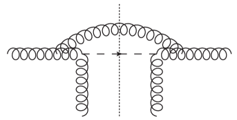
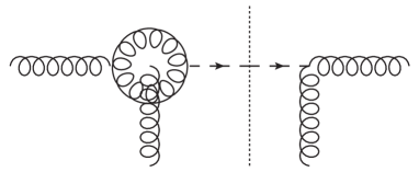
Figure 1: Examples of one-loop diagrams from the real gluon radiation (L) and virtual gluon radiation (R) for the scalar particle production in $pA$ collisions in the saturation formalism with the multiple interactions with the nucleus target taken into account. Here the vertical gluon represents arbitrary number of the WW small-$x$ gluons which are summed into Wilson lines.

At one-loop order, real and virtual diagrams yield higher order corrections which contain various divergences. In addition to the rapidity divergence associated with the WW gluon distribution from the nucleus, there is also the collinear divergence for the integrated gluon distribution from the nucleon. In our calculations, the dimensional regulation ($D=4-2\epsilon$) is used to formulate the collinear divergence, whereas the direct subtraction is applied for the rapidity divergence. In Fig. 1, we plot the typical diagrams from the real and virtual gluon radiations at one-loop order . The scattering amplitude from the real diagrams can be written as,

$${\cal A}^{\nu\alpha} = \int\frac{d^{2}k_{g1\perp}}{(2\pi)^{2}}\frac{zk_{1\perp}^{\alpha}g^{\nu\beta}+(1-z)k_{1\perp}^{\beta}g^{\alpha\nu}-z(1-z)k_{1\perp}^{\nu}g^{\alpha\beta}}{k_{1\perp}^{2}}\Gamma_{A}^{\beta}(k_{g1\perp},k_{g2\perp})$$ (3)

$$+\left[\left(\frac{zk_{\perp}^{\prime\alpha}k_{\perp}^{\prime\nu}}{k_{\perp}^{\prime 2}+\epsilon_{f}^{2}}-\frac{zk_{\perp}^{\alpha}k_{\perp}^{\nu}}{k_{\perp}^{2}+\epsilon_{f}^{2}}\right)+z(1-z)Q^{2}\frac{g^{\alpha\nu}}{2}\left(\frac{1}{k_{\perp}^{2}+\epsilon_{f}^{2}}-\frac{1}{k_{\perp}^{\prime 2}+\epsilon_{f}^{2}}\right)\right]\Gamma_{B}(k_{g\perp})\ ,$$

where $k_{\perp}$ and $k_{2\perp}$ represent the transverse momenta for the final state scalar particle and the radiated gluon, respectively, $k_{g\perp}=k_{g1\perp}+k_{g2\perp}=k_{\perp}+k_{2\perp}$, $\epsilon_{f}^{2}=(1-z)Q^{2}$ with $z$ the momentum fraction of the incoming gluon carried by the scalar particle. For convenience, we further define $k_{1\perp}=k_{\perp}-k_{g1\perp}$, $k_{\perp}^{\prime}=k_{\perp}-zk_{g\perp}$, and $\nu$ and $\alpha$ are the polarization vector indices for the incoming and outgoing gluons, for which we have chosen the physical polarizations. $\Gamma_{A}$ and $\Gamma_{B}$ are defined as

$$\Gamma_{A}^{\beta}(k_{g1\perp},k_{g2\perp}) = \int d^{2}x_{1}d^{2}x_{2}e^{ik_{g1\perp}\cdot x_{1}+ik_{g2\perp}\cdot x_{2}}{\rm Tr}\left[U^{\dagger}(x_{2})T^{b}U(x_{2})[i\partial_{\perp}^{\beta}U^{\dagger}(x_{1})U(x_{1}),T^{a}]\right]\ ,$$ (4)

$$\Gamma_{B}(k_{g\perp}) = 2\int d^{2}x_{\perp}e^{ik_{g\perp}\cdot x_{\perp}}{\rm Tr}\left[T^{b}U(x_{\perp})T^{a}U^{\dagger}(x_{\perp})\right]\ ,$$ (5)

where $a$ and $b$ are color indices for the incoming and outgoing gluons, respectively. Clearly, the amplitude squared from the above expressions will depend on multi-gluon correlation functions (beyond the WW-gluon distribution) from the nucleus, as this is the common feature in the high order calculations in the small-$x$ formalism Metz:2011wb . However, in the $k_{\perp}\ll Q$ limit, these correlation functions is either reduced to the WW-gluon distribution, or absorbed into the evolution of the WW-gluon distribution. To evaluate the contribution from the real gluon radiation, we integrate out the phase space of the radiated gluon ($k_{2}$). To simplify the calculation, we perform the power expansion of the amplitude squared in terms of $k_{\perp}/Q$, and only keep the leading power contributions. In the power counting analysis, we find that the phase space integral contains three important contributions: (1) soft gluon radiation $k_{2}^{+}\sim k_{2}^{-}\sim k_{2\perp}$ which eventually leads to the Sudakov logarithms; (2) collinear gluon contribution as respect to the incoming nucleon projectile; (3) collinear gluon contribution as respect to the target nucleus. The soft gluon contribution can be easily obtained in the limit of $Q^{2}\gg k_{\perp}^{2}$, which results into $\delta(k_{2}^{+})\delta(k_{2}^{-})\ln({Q^{2}}/{k_{2\perp}^{2}})$. When Fourier transformed into the impact parameter space, this term leads to a soft divergence in terms of $1/\epsilon^{2}$ in dimension regulation. The soft divergence will be cancelled by the relevant virtual diagrams. The last contribution contains the rapidity divergence and gives rise to the evolution of the WW gluon distribution.

The evaluation of the virtual diagrams leads to the following contributions,

$$-\alpha_{s}\int\frac{dz}{z(1-z)}\frac{d^{2}q_{\perp}d^{2}k_{g1\perp}}{(2\pi)^{4}}\Gamma_{C}(k_{g1\perp},k_{g2\perp})\left[\frac{k_{g1\perp}^{\nu}}{q_{\perp}^{2}}-\frac{2q_{\perp}^{\prime\nu}q_{\perp}\cdot q_{\perp}^{\prime}-q_{\perp}^{\nu}q_{\perp}^{\prime 2}}{q_{\perp}^{2}(q_{\perp}^{\prime 2}+\epsilon_{f}^{\prime 2})}\right]$$

$$+\frac{\alpha_{s}N_{c}}{\pi}\beta_{0}\left(\frac{1}{\epsilon_{UV}}-\frac{1}{\epsilon_{IR}}\right)\Gamma_{D}(k_{\perp})\ ,$$ (6)

where $\epsilon_{f}^{\prime 2}=-z(1-z)Q^{2}$, $q_{\perp}^{\prime}=q_{\perp}+k_{g1\perp}-zk_{\perp}$ with $k_{\perp}=k_{g1\perp}+k_{g2\perp}$, $\beta_{0}=11/12-N_{f}/18$ with $N_{f}$ number of flavors, $\epsilon_{UV}$ and $\epsilon_{IR}$ represent the ultra-violet and infrared divergences in the loop diagrams, respectively, and $\Gamma_{C}$ and $\Gamma_{D}$ are defined as

$$\Gamma_{C}(k_{g1\perp},k_{g2\perp}) = \int d^{2}x_{1}d^{2}x_{2}e^{ik_{g1\perp}\cdot x_{1}+ik_{g2\perp}\cdot x_{2}}$$ (7)

$$\times\left\{{\rm Tr}\left[U(x_{1})T^{a}U^{\dagger}(x_{2})\right]{\rm Tr}\left[U^{\dagger}(x_{1})U(x_{2})\right]-(x_{1}\leftrightarrow x_{2})\right\}\ ,$$

$$\Gamma_{D}^{\beta}(k_{\perp}) = \int d^{2}xe^{ik_{g\perp}\cdot x_{\perp}}{\rm Tr}\left[T_{a}i\partial_{\perp}^{\beta}U^{\dagger}(x_{\perp})U(x_{\perp})\right]\ .$$ (8)

In Eq. (6), the ultra-violet (UV) divergences cancel out between the two contributions in the first term, whereas the remaining UV-divergence in the second term is normally interpreted as the charge renormalization, which appears in the form of $({\alpha_{s}}/{\pi})N_{c}\beta_{0}\left(-{1}/{\epsilon_{UV}}+\ln({Q^{2}}/{\mu^{2}})\right)$. Furthermore, there is also IR divergence, which can be absorbed into the renormalization for the incoming gluon distribution from the nucleon. In addition, there are rapidity divergence and soft divergence in the first term of Eq. (6). The soft divergence is regulated by dimension regularization, and is found to proportional to $1/\epsilon^{2}$. This divergence, as mentioned above, will cancel out that from the real diagrams.

After canceling out the soft divergences from the real and virtual diagrams, we are left with the rapidity divergence and collinear divergence,

$$xg_{p}(x)\int\frac{d\xi}{\xi}{\bf K}_{\rm DMMX}\otimes S^{WW}(x_{\perp},y_{\perp})+\left(-\frac{1}{\epsilon}\right)\frac{\alpha_{s}N_{c}}{\pi}S^{WW}(x_{\perp},y_{\perp}){\cal P}_{g/g}\otimes xg_{p}(x)\ ,$$ (9)

where ${\bf K}_{\rm DMMX}$ is the BK-type of evolution kernel for the WW gluon distribution, and ${\cal P}_{g/g}=\frac{1}{(1-z)_{+}}+\frac{1}{z}+z(1-z)+\beta_{0}\delta(1-z)$ the collinear evolution kernel for the incoming gluon from the nucleon. Our result for ${\bf K}_{\rm DMMX}$ is consistent with a recent calculation for the evolution directly from the JIMWLK evolution Dominguez:2011gc . After subtracting these divergences by the renormalizations of the associated distributions, we obtain the final result for the differential cross section as

$$\frac{d\sigma^{\rm(LO+NLO)}}{dyd^{2}k_{\perp}}|_{k_{\perp}\ll Q} = \sigma_{0}\int\frac{d^{2}x_{\perp}d^{2}x_{\perp}^{\prime}}{(2\pi)^{2}}e^{ik_{\perp}\cdot r_{\perp}}S^{WW}_{Y=\ln 1/x_{a}}(x_{\perp},x_{\perp}^{\prime})xg_{p}(x,\mu^{2}=\frac{c_{0}^{2}}{r_{\perp}^{2}})$$ (10)

$$\left\{1+\frac{\alpha_{s}}{\pi}N_{c}\left[\beta_{0}\ln\frac{Q^{2}r_{\perp}^{2}}{c_{0}^{2}}-\frac{1}{2}\left(\ln\frac{Q^{2}r_{\perp}^{2}}{c_{0}^{2}}\right)^{2}+\frac{\pi^{2}}{2}\right]\right\}\ ,$$

where $c_{0}=2e^{-\gamma_{E}}$ with $\gamma_{E}$ the Euler constant. We have also introduced the scale for the integrated gluon distribution $\mu^{2}=c_{0}^{2}/r_{\perp}^{2}$ and the rapidity for the WW gluon $Y=\ln 1/x_{a}$ to simplify the above expression.

Comparing to the differential cross section calculation for inclusive hadron production in $pA$ collisions Chirilli:2011km , we find that they share the same structure. In particular, the integrated parton distribution is more convenient to be set at the scale of $c_{0}/r_{\perp}$. The major difference is that, the above formula is valid in the limit of $Q\gg k_{\perp}$ where we have to resum the Sudakov logarithms. That is also the reason that the un-integrated gluon distribution from the nucleus side does not depend on more complicated structure of the Wilson lines. If we calculate the differential cross section in the kinematic region of $k_{\perp}\sim Q$, the multi-gluon correlation functions (beyond the WW-gluon distribution) from the nucleus will contribute, similar to what was found in Ref. Chirilli:2011km . Those contributions, however, is power suppressed in the limit of $k_{\perp}\ll Q$.

We have also performed this calculation in coordinate space with cutoffs putting into integrals instead of the use of the dimensional regularization, and obtained the same results. This implies that there is no scheme dependence in the Sudakov logarthms, at least to the level we are concerned.

3. All Order Resummation. Our calculations at one-loop order in the above demonstrate that the soft gluon radiation is well separated from the collinear gluon radiations. In particular, the soft gluon radiation comes from the initial state radiation, and in the $Q\gg k_{\perp}$ limit, the relevant gluon distribution from the nucleus takes the form of the WW gluon distribution. Higher order soft gluon radiations will follow the same form. This can be understood that the Sudakov double logarithms come from soft gluon radiation associated with the hard probe. To resum these large logarithms, we follow the Collins-Soper-Sterman procedure Collins:1984kg . In particular, we can write down an evolution equation respect to the hard scale $Q^{2}$. By solving the differential equation, we can resum the differential cross section in terms,

$$\frac{d\sigma^{\rm({\rm resum})}}{dyd^{2}k_{\perp}}|_{k_{\perp}\ll Q} = \sigma_{0}\int\frac{d^{2}x_{\perp}d^{2}x_{\perp}^{\prime}}{(2\pi)^{2}}e^{ik_{\perp}\cdot r_{\perp}}e^{-{\cal S}_{sud}(Q^{2},r_{\perp}^{2})}S^{WW}_{Y=\ln 1/x_{a}}(x_{\perp},x_{\perp}^{\prime})$$ (11)

$$\times xg_{p}(x,\mu^{2}={c_{0}^{2}}/{r_{\perp}^{2}})\left[1+\frac{\alpha_{s}}{\pi}\frac{\pi^{2}}{2}N_{c}\right]\ ,$$

where the Sudakov form factor contains all order resummation

$${\cal S}_{sud}=\int_{C_{1}^{2}/r^{2}}^{C_{2}^{2}Q^{2}}\frac{d\mu^{2}}{\mu^{2}}\left[A\ln\frac{C_{2}^{2}Q^{2}}{\mu^{2}}+B\right]\ ,$$ (12)

where $C_{1,2}$ are parameters in order of 1. The hard coefficients $A$ and $B$ can be calculated perturbatively: $A=\sum\limits_{i=1}^{\infty}A^{(i)}\left(\frac{\alpha_{s}}{\pi}\right)^{i}$. From the explicit results for the one-loop calculations, we find that they are

$$A^{(1)}=N_{c},~{}~{}~{}B^{(1)}=-\beta_{0}N_{c}\ ,$$ (13)

where we have chosen the so-called canonical variables for $C_{1}=c_{0}$ and $C_{2}=1$. The above formulas are the final results for the soft gluon resummation in massive scalar particle production in $pA$ collisions. The result is valid in the limit of $k_{\perp}\ll Q$, and we have applied the small-$x$ factorization where higher order in $1/\ln(1/x_{a})$ has been neglected as well. As compared to Ref. Ji:2005nu which takes the $\alpha_{s}$ correction of $g_{\phi}$ into account, we find the above coefficients are consistent with the known resultsBerger:2002ut except for $B^{(1)}$ which misses a factor of 2. This difference is due to the convention in the saturation formalism in which we do not include the virtual gluon and quark loops contribution for the vertical WW small-$x$ gluons as shown in Fig. 1.

We would like to emphasize a number of important features in the above derivation. First, the collinear divergence and the soft divergence is well separated. This follows the transverse momentum resummation in the collinear factorization. Second and most importantly, the rapidity divergence from the the un-integrated gluon distribution of the nucleus is also well separated from the soft gluon radiation. This is because the rapidity divergence comes form the collinear gluon radiation parallel to the nuclei momentum, whereas the Sudakov logarithms come from soft gluon region.

Third, as the above features are common features in the small-$x$ saturation formalism, we expect our resummation results can be extended to other hard processes. An immediate application is the color neutral particle production in $pA$ collisions, such as the two-photon production Qiu:2011ai and heavy quarkonium production Sun:2012vc . There are only initial state interactions in these processes, and the Sudakov resummation will be the same as what we have derived in this paper for the massive scalar particle production. We expect the similar resummation formula. Another important extension is the dijet correlation in $pA$ collisions Dominguez:2010xd , which has attracted great attentions in recent years. Of course, because the final state of dijet production carries color, we have to take into account the final state interaction effects in the Sudakov resummation. Therefore, the resummation formula will be different from the scalar particle production studied in this paper. However, the generic form will remain the same. We plan to address this calculation in a future publication.

4. Discussions and Conclusion. In summary, we have demonstrated the Sudakov double logarithms in the small-$x$ calculations of hard processes in $pA$ collisions. All order resummation formalism has been derived. This result will have potential application for other hard processes in $pA$ collisions, from which we hope to investigate the saturation physics.

In addition, the technique developed in this paper shall also be relevant for the hard processes in hot/dense medium, such as the quark-gluon plasma. In particular, in the hard processes of jet penetrating through the medium, we expect the similar formalism for the Sudakov resummation effects. The direct consequence is that the transverse momentum broadening in the hard processes (with hard momentum scale much larger than the momentum scale in the medium) will be dominated by the Sudakov logarithms which is the same as that in the vacuum. This may lead to a natural explanation for the azimuthal angle correlation of dijet production in heavy ion collisions which was found the same as that in $pp$ collisions in the large angle region Aad:2010bu , where Sudakov effects dominate.

This work was supported in part by the U.S. Department of Energy under the contracts DE-AC02-05CH11231 and DOE OJI grant No. DE - SC0002145. We thank J. W. Qiu for comments and discussions.

References

- (1) V. V. Sudakov, Sov. Phys. JETP 3, 65 (1956) [Zh. Eksp. Teor. Fiz. 30, 87 (1956)]; Y. L. Dokshitzer, D. Diakonov and S. I. Troian, Phys. Rept. 58, 269 (1980); G. Parisi and R. Petronzio, Nucl. Phys. B 154, 427 (1979).
- (2) J. C. Collins, D. E. Soper and G. F. Sterman, Nucl. Phys. B 250, 199 (1985).
- (3) I. I. Balitsky and L. N. Lipatov, Sov. J. Nucl. Phys. 28, 822 (1978) [Yad. Fiz. 28, 1597 (1978)]; E. A. Kuraev, L. N. Lipatov and V. S. Fadin, Sov. Phys. JETP 45, 199 (1977) [Zh. Eksp. Teor. Fiz. 72, 377 (1977)].
- (4) L. V. Gribov, E. M. Levin and M. G. Ryskin, Phys. Rept. 100, 1 (1983).
- (5) A. H. Mueller and J. W. Qiu, Nucl. Phys. B 268, 427 (1986).
- (6) L. D. McLerran and R. Venugopalan, Phys. Rev. D 49, 2233 (1994); Phys. Rev. D 49, 3352 (1994).
- (7) I. Balitsky, Nucl. Phys. B463, 99-160 (1996); Y. V. Kovchegov, Phys. Rev. D60, 034008 (1999).
- (8) J. Jalilian-Marian, A. Kovner, A. Leonidov and H. Weigert, Nucl. Phys. B 504, 415 (1997); J. Jalilian-Marian, A. Kovner, A. Leonidov and H. Weigert, Phys. Rev. D 59, 014014 (1998).
- (9) E. Iancu, A. Leonidov and L. D. McLerran, Nucl. Phys. A 692, 583 (2001); Nucl. Phys. A 703, 489 (2002).
- (10) D. Boer, et al., arXiv:1108.1713; J. L. Abelleira Fernandez et al. arXiv:1206.2913.
- (11) F. Dominguez, B. W. Xiao and F. Yuan, Phys. Rev. Lett. 106, 022301 (2011); F. Dominguez, C. Marquet, B. W. Xiao and F. Yuan, Phys. Rev. D 83, 105005 (2011).
- (12) S. Dawson, Nucl. Phys. B 359, 283 (1991); A. Djouadi, M. Spira and P. M. Zerwas, Phys. Lett. B 264, 440 (1991).
- (13) A. H. Mueller, Nucl. Phys. B 335, 115 (1990); Nucl. Phys. B 415, 373 (1994); Y. V. Kovchegov and A. H. Mueller, Nucl. Phys. B 529, 451 (1998).
- (14) G. A. Chirilli, B. -W. Xiao and F. Yuan, Phys. Rev. Lett. 108, 122301 (2012); Phys. Rev. D 86, 054005 (2012).
- (15) A. Metz and J. Zhou, Phys. Rev. D 84, 051503 (2011); D. Boer, W. J. den Dunnen, C. Pisano, M. Schlegel and W. Vogelsang, Phys. Rev. Lett. 108, 032002 (2012); P. Sun, B. -W. Xiao and F. Yuan, Phys. Rev. D 84, 094005 (2011); A. Schafer and J. Zhou, Phys. Rev. D 85, 114004 (2012); T. Liou, arXiv:1206.6123 [hep-ph].
- (16) F. Dominguez, A. H. Mueller, S. Munier and B. -W. Xiao, Phys. Lett. B 705, 106 (2011).
- (17) X. Ji, J. P. Ma and F. Yuan, JHEP 0507, 020 (2005).
- (18) E. L. Berger and J. -w. Qiu, Phys. Rev. D 67, 034026 (2003).
- (19) J. -W. Qiu, M. Schlegel and W. Vogelsang, Phys. Rev. Lett. 107, 062001 (2011).
- (20) P. Sun, C. -P. Yuan and F. Yuan, arXiv:1210.3432 [hep-ph].
- (21) G. Aad et al. [Atlas Collaboration], Phys. Rev. Lett. 105, 252303 (2010); S. Chatrchyan et al. [CMS Collaboration], Phys. Rev. C 84, 024906 (2011).