Experimental characterization of railgun-driven supersonic plasma jets motivated by high energy density physics applications

Abstract

We report experimental results on the parameters, structure, and evolution of high-Mach-number ($M$) argon plasma jets formed and launched by a pulsed-power-driven railgun. The nominal initial average jet parameters in the data set analyzed are density $\approx 2\times 10^{16}$ cm^-3, electron temperature $\approx 1.4$ eV, velocity $\approx 30$ km/s, $M\approx 14$, ionization fraction $\approx 0.96$, diameter $\approx 5$ cm, and length $\approx 20$ cm. These values approach the range needed by the Plasma Liner Experiment (PLX), which is designed to use merging plasma jets to form imploding spherical plasma liners that can reach peak pressures of 0.1–1 Mbar at stagnation. As these jets propagate a distance of approximately 40 cm, the average density drops by one order of magnitude, which is at the very low end of the 8–160 times drop predicted by ideal hydrodynamic theory of a constant-$M$ jet.

I Introduction

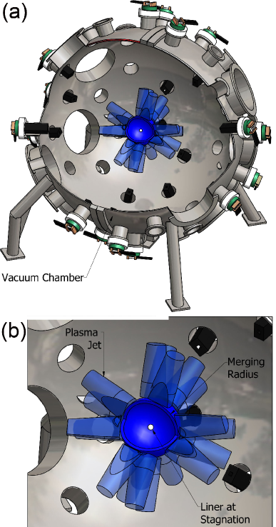
Figure 1: (a) Schematic of the Plasma Liner Experiment (PLX), designed as a thirty plasma jet experiment to form spherically imploding plasma liners. This paper reports single jet characterization and propagation studies. (b) Illustration of imploding spherical plasma liner formation via the merging of thirty jets, and also the stagnated liner at peak compression (later in time).

This paper reports results from the first in a series of planned/proposed experiments to demonstrate the formation of imploding spherical plasma liners via an array of merging high-Mach-number ($M$) plasma jets. Results are obtained on the Plasma Liner Experiment (PLX), depicted in Fig. 1, at Los Alamos National Laboratory. Imploding spherical plasma liners have been proposedThio et al. (1999, 2001); Hsu et al. (2012) as a standoff compression driver for magneto-inertial fusion (MIF)Lindemuth and Kirkpatrick (1983); Kirkpatrick, Lindemuth, and Ward (1995); Lindemuth and Siemon (2009) and, in the case of targetless implosions, for generating cm-, $\mu$s-, and Mbar-scale plasmas for high energy density (HED) physicsDrake (2010) research. Several recent theoretical and computational studies have investigated the physics of imploding spherical plasma liner formationParks (2008); Cassibry et al. (2009); Awe et al. (2011); Cassibry et al. (2012); Kim et al. (2012); Davis et al. (2012); Cassibry, Stanic, and Hsu and also the fusion energy gain of plasma liner driven MIF.Parks (2008); Cassibry et al. (2009); Samulyak, Parks, and Wu (2010); Santarius (2012); Kim et al. (2012) In this work, we provide a detailed experimental characterization of high-$M$ argon plasma jet propagation. In a forthcoming paper we will present the experimental characterization of two such jets merging at an oblique angle. The next step, a thirty-jet experiment to form spherically imploding plasma liners that reach 0.1–1 Mbar of peak pressure at stagnation, has been designedHsu et al. (2012); Cassibry, Stanic, and Hsu but not yet fielded. The primary objective of the single-jet propagation and two-jet oblique merging studies is to obtain critical experimental data in order to (1) uncover important unforeseen issues and (2) provide inputs to and constraints on numerical modeling efforts aimed at developing predictive capability for the performance of imploding spherical plasma liners.

This study focuses on addressing issues for the potential use of railgun-driven high-$M$ plasma jets for forming imploding spherical plasma liners and the ability to reach HED-relevant stagnation pressures ($\gtrsim 1$ Mbar). Thus, we are interested not only in the jet parameters as they exit the railgun, but also in the evolution of the plasma jet as it propagates a distance of $\sim 0.5$ m, as this evolution will affect subsequent jet merging and ultimately the plasma liner formation and implosion processes. As such, our work constitutes a unique contribution to the large body of railgun research,thi which has primarily focused on the dynamics and performance of the “armature”Thio and Frost (1986); Parker (1989); Batteh (1991) within the railgun bore and the ability of railguns to launch solid projectiles or develop thrust for militaryMcNab and Beach (2007) and space applications.Jahn (1968); zie ; McNab (2009) These jets, if injected into a tokamak plasma, may also find applications in core re-fueling or edge-localized-mode (ELM) pacing.Voronin et al. (2005); Liu and Hsu (2011)

The remainder of the paper is organized as follows: Sec. II gives a brief overview of the physical steps of imploding spherical plasma liner formation using merging plasma jets, and summarizes key recognized issues (focusing on jet propagation prior to jet merging); Sec. III describes the experimental setup and diagnostics; Sec. IV presents the experimental results on plasma jet parameters, structure, and evolution; and Sec. V provides conclusions and a summary.

II Use of plasma jets for forming imploding spherical plasma liners

II.1 Steps of plasma liner formation

Here, we provide a brief summary of the steps in imploding plasma liner formation using an array of merging plasma jets. Much more detailed accounts, including both theoretical and computational results, have been presented elsewhere.Parks (2008); Hsu et al. (2012); Cassibry, Stanic, and Hsu

First, multiple plasma jets are launched radially inward from the periphery of a large spherical vacuum chamber. The jets propagate separately until they coalesce at the merging radius $R_{m}$, which depends on the jet $M$, the number of jets $N$, the initial jet radius $r_{j0}$, and the chamber radius $R_{w}$. For non-varying $M$ and the assumption of a jet radial expansion speed of $2C_{s}/(\gamma-1)$,Landau and Lifshitz (1987) where $C_{s}$ is the ion sound speed and $\gamma$ is the polytropic index, $R_{m}$ has been derived asCassibry et al. (2012)

$$R_{m}=\frac{r_{j0}\left(M\frac{\gamma-1}{2}+1\right)+R_{w}}{1+\frac{2}{N^{1/2}}\left(M\frac{\gamma-1}{2}+1\right)}.$$ (1)

Note that as $M\rightarrow\infty$ (i.e., no radial jet expansion), $R_{m}\rightarrow N^{1/2}r_{j0}/2$. For PLX-relevant values ($M=14$, $N=30$, $r_{j0}=2.5$ cm, $R_{w}=111$ cm, $\gamma=1.4$), $R_{m}\approx 50$ cm, meaning that the jets will propagate about 60 cm before merging with adjacent jets. The reduced value of $\gamma=1.4$ (below the ideal gas value of $5/3$) is used throughout the paper to approximate the internal degrees of freedom of an argon plasma, i.e., due to ionizations and excitations.Murakami and Nishihara (2000); Awe et al. (2011) If $M$ increases during jet propagation due to radiative cooling, then Eq. (1) overestimates $R_{m}$ and underestimates the jet propagation distance before merging. Nevertheless, for PLX, we are interested in jet propagation distances of order 0.5 m. Characterizing the evolution of jet parameters over that distance is the focus of this paper.

Adjacent jets merge at oblique angles at $R_{m}$ to form an imploding spherical plasma liner. For PLX, the jet merging angles are determined by the vacuum chamber port positions, with nearest neighbor jets meeting at $\theta=24^{\circ}$. Even at this angle, two adjacent jets, each with $M=14$, meet with a relative Mach number of $2M\sin(\theta/2)\approx 6$. Thus, shock formation and associated heating may be expected to contribute significant non-uniformities to the plasma liner formation process. The strength of the shock, and indeed whether shocks even form, are open research questions due to the parameter regime of our jets,Hsu et al. (2012); Ryutov et al. (2012) i.e., the plasma within each jet is highly collisional (argon ion mean free path $\lambda_{i}\approx 4\times 10^{-4}$ cm compared to the jet diameter of 5–20 cm, where $n_{i}=2\times 10^{16}$ cm^-3, $T_{i}=1.4$ eV, and mean charge state $Z_{eff}=1$ have been used to estimate $\lambda_{i}$) but the interaction between two jets is semi-collisional or even collisionless (due to the high relative velocity between the jets) on the scale of the jet diameter. Shock heating, should it occur, may degrade the implosion Mach number, which would lead to the undesirable result of lower liner stagnation pressure.Awe et al. (2011); Davis et al. (2012) The non-uniformities introduced by discrete jet merging may lead to asymmetries in the plasma liner implosion that significantly degrade the peak achievable stagnation pressures. These and other issues relating to plasma liner formation via discrete merging plasma jets have been studied theoreticallyParks (2008) and computationallyCassibry et al. (2012) elsewhere and are beyond the scope of this paper. Experimental results from PLX on two-jet oblique merging will be presented in a forthcoming paper.

Finally, after all the jets merge into an imploding spherical plasma liner, the liner converges with mass density $\rho\sim\rho_{0}R^{-2}$, where $\rho_{0}$ is the mass density at $R_{m}$ and $R$ is the radial position of the imploding liner.Parks (2008); Samulyak, Parks, and Wu (2010); Awe et al. (2011) This results in the convergent amplification of liner ram pressure until the liner reaches the origin and stagnates (for targetless liner implosions), converting the liner kinetic energy into stagnation thermal energy and excitation/ionization energy of the liner plasma.Davis et al. (2012) An outward-propagating shock is launched, and when this shock meets the trailing edge of the incoming liner, the entire system disassembles after a stagnation time $\tau_{stag}\sim L_{j0}/V_{j0}$,Awe et al. (2011); Davis et al. (2012) where $L_{j0}$ and $V_{j0}$ are the initial jet length and velocity, respectively.

II.2 Issues relating to jet propagation

There are several issues relating to jet propagation that are important for determining the performance of the subsequent liner formation, implosion, and stagnation. Assessing these issues experimentally is the primary motivation for this single-jet study. In all cases, the experimental results are intended to improve the predictive capability of imploding spherical plasma liner modeling.

The first issue is the achievement of the requisite jet parameters for reaching the desired liner stagnation pressure. The design goal for PLX is to reach 0.1–1 Mbar with a total liner kinetic energy of about 375 kJ. A 3D ideal hydrodynamic simulation studyCassibry, Stanic, and Hsu exploring a wide parameter space in plasma jet initial conditions contributed to the PLX reference design calling for thirty argon plasma jets with initial density $\approx 10^{17}$ cm^-3, velocity $\approx 50$ km/s, and mass $\approx 8$ mg. The simultaneous achievement of these parameters has recently been demonstrated at HyperV Technologies, to be reported elsewhere. For this paper, we operated at reduced values to extend the lifetime of the railgun and maximize the number of shots. The second issue is the evolution of jet parameters, especially density and velocity, during propagation. Developing an accurate predictive capability for modeling plasma liner formation via merging jets requires accurate knowledge of these jet parameters, both at the exit of the railgun as well as at $R_{m}$. The jet velocity is expected to remain nearly constant, but density decay arises from jet radial and axial expansion. The third issue is the nature of the jet radial and axial profiles because they are important for accurate modeling of the jet merging and liner formation/implosion processes.

Experimental values (presented in Sec. IV) allow the jet expansion to be estimated. In a purely hydrodynamic treatment in which the jet has a non-varying $M$, both the radial and axial expansion speeds of the jet can be estimated to be between $C_{s}$ (jet bulk) and $2C_{s}/(\gamma-1)$ (jet edges).Landau and Lifshitz (1987) For argon at $T_{e}=1.4$ eV and $\gamma=1.4$, these values are 2.2 km/s and 11 km/s, respectively. If the jet travels at 30 km/s over a distance of 50 cm, this gives a transit time of 16.7 $\mu$s, during which the jet radius will increase by 3.7–16.7 cm and the jet length by 7.4–33.4 cm. For a jet with $r_{j0}=2.5$ cm and $L_{j0}=20$ cm, the jet volume will increase by a factor of 8.4–157.5, and the density will drop by the same factor. Due to the nearly factor of twenty uncertainty in the theoretically predicted density decay, and the fact that jet cooling due to expansion and radiative losses (and thus a varying rate of expansion) are not accounted for in the above treatment, it is imperative to determine the density decay by direct experimental measurement.

III Experimental setup

III.1 Plasma Liner Experiment (PLX)

Experiments on PLX are conducted in a 9 ft. (2.74 m) diameter stainless steel spherical vacuum chamber, as depicted in Fig. 1(a), situated in a 3000 ft.² (279 m²) high-bay space with a ten-ton overhead crane. The vacuum chamber has 60 smaller ports (11 in. outer and $7\frac{3}{4}$ in. inner diameters) and 10 larger ports (29.5 in. outer and 23.5 in. inner diameters); all flanges are aluminum. We presently have two operational plasma railguns (see Sec. III.2 for railgun specifications) installed on the vacuum chamber to study high-$M$ single-jet propagation, two-jet oblique merging, and two-jet head-on merging. This paper reports only single jet results. The vacuum base pressure is typically in the low-$10^{-6}$ Torr range, achieved with a turbo-molecular pump (3200 l/s Leybold Mag W 3200C, $12\frac{3}{4}$ in. pumping diameter) backed by an oil-free mechanical pump (Edwards IQDP 80). During each experimental shot, the turbo-pump is isolated by closing a gate valve, and thus the vacuum pressure is in the 5–30 $\mu$Torr range when a plasma jet is fired into the chamber. The pressure in the chamber after a shot is in the 0.3-to-few mTorr range; the gate valve is opened and the chamber evacuated prior to the next shot. All chamber pressures are recorded using an MKS 972B DualMag transducer. A LabVIEW-based (http://www.ni.com/labview) 40 MHz field programmable gate array (FPGA) system controls safety interlocks, shot sequence including bank charging and dumping, and all trigger signals. Sensitive control and data acquisition electronics reside within an electromagnetically shielded cage or other shielded racks. All time-series data shown in this paper were digitized at 40 MHz sampling rate, 12-bit dynamic range, and 1 mV bit resolution (by Joerger model TR digitizers). All times reported in the paper are relative to the trigger time of the gun rails. Experimental data and shot data are immediately stored into an MDSplus (http://www.mdsplus.org) database after every shot.

III.2 Plasma railgun

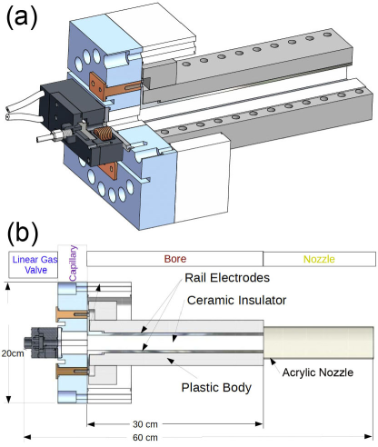
Figure 2: (a) Three-dimensional view of the railgun used in this work. (b) Side-view schematic of railgun showing (from left to right): fast gas valve, capillary (pre-ionizer), bore (HD-17 tungsten alloy rails with zirconium-strengthened-alumina insulators), and acrylic nozzle. The distance from the back of the rails to the end of the nozzle is 47 cm.

To achieve the design objectives of PLX (i.e., 0.1–1 Mbar of peak liner stagnation pressure using thirty plasma jets with total implosion kinetic energy of $\sim 375$ kJ) within budgetary constraints, two-stage parallel-plate railguns (see Fig. 2), designed and fabricated by HyperV Technologies Corp.,Witherspoon et al. (2011) were selected as the plasma gun source for forming and launching jets with the requisite parameters (jet density $\approx 10^{17}$ cm^-3, velocity $\approx 50$ km/s, and mass $\approx 8$ mg). The development, optimization, and performance scaling results of these PLX railguns, as well as the simultaneous experimental achievement of the aforementioned jet parameters, will be reported elsewhere. Note that larger coaxial guns with shaped electrodesWitherspoon et al. (2009); Messer et al. (2009); Case et al. (2010) are also being developed due to their suitability for very high current ($>1$ MA) and high jet velocity ($>100$ km/s) operation, and for having attributes that minimize impurities, as potentially required for the MIF application.

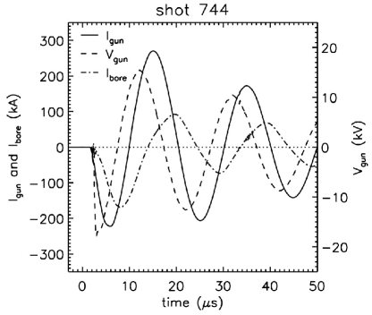
Figure 3: Representative railgun $I_{gun}$, $V_{gun}$, and gun bore current $I_{bore}$ (near the rear of the rails) for the shots analyzed in this paper.

The railgun bore cross-sectional area is $2.54\times 2.54$ cm². The gun has a fast gas-puff valve (GV), a pre-ionizer (PI), HD-17 (tungsten alloy) rails housed in a Noryl (blend of polyphenylene oxide and polystyrene) clamshell body, zirconium toughened alumina (ZTA) insulators between the rails, and a cylindrical acrylic nozzle (5 cm diameter and 19 cm length). The results reported here are from shots with an underdamped, ringing, and slowly decaying gun current (Fig. 3) that produces multiple jet structures, with the leading structure having a length of order 20 cm. We use ultra-high-purity argon (typically at 18–20 psig) for the gas injection, injecting an average total mass of about 35 mg in each shot for the data set presented in this paper (but only a small fraction of the total injected mass is contained in the leading jet structure).

The railgun firing sequence is GV followed by the PI and finally the rails. The time delays are all adjustable and are chosen for optimizing certain aspects of jet performance such as density, velocity, or mass. For the shots reported here, the GV is fired 300 $\mu$s before the gun rails so that neutral argon fills the PI volume and the very rear of the railgun bore. The PI is fired 30 $\mu$s before the gun rails to break down the neutral gas, giving the PI plasma just enough time to fill the very rear of the railgun bore. Then the rails are fired to accelerate the PI plasma down the bore. Control over the plasma jet density and mass is mainly through the feed line pressure, GV bank voltage, and timing of the neutral gas puff; control over the jet velocity is mainly through the railgun current and charge voltage. For single-gun operation, the gun, PI, and GV are driven by 36 $\mu$F, 6 $\mu$F, and 24 $\mu$F capacitor banks, respectively, charged typically to -24 kV, 20 kV, and 8 kV, respectively. The 36 and 6 $\mu$F banks use 60-kV, 6-$\mu$F Maxwell model 32184 capacitors, and the 24-$\mu$F bank uses a single 50-kV Maxwell model 32567 capacitor. All banks are switched by spark-gap switches triggered via optical fibers. Details about the gun design, operation, performance scaling, and best achieved parameters will be reported elsewhere.

We have evidence that the plasma jet is not 100% argon. We observe an approximately 25% higher pressure rise in the chamber (for the data set presented in this paper) when the GV and railgun are both fired, compared to when only the GV is fired. The pressure discrepancy is most likely explained by the railgun current ablating material from the HD-17 rails and possibly also the ZTA insulators. We also observe hydrogen, oxygen, and aluminum impurity spectral lines, and potentially others that have not yet been identified (with tungsten, nickel, iron, and copper from the rails as likely candidates). In the remainder of the paper, we have assumed that the plasma jets are 100% argon for the purpose of interpreting the experimental data because the error introduced is generally small compared to diagnostic measurement uncertainties. Impurity control in plasma jets is clearly an important issue for the MIF standoff driver application and requires further study.

III.3 Diagnostics

Plasma jet diagnostics include an eight-chord interferometer, a visible and near-infrared (IR) survey spectrometer, an array of three photodiode detectors, and an intensified CCD (charge-coupled device) imaging camera. Details of each plasma jet diagnostic system are given below. Figure 4 shows the diagnostic views in relation to the plasma jet propagation path. A discussion of the entire planned PLX diagnostic suite is described in more detail elsewhere.Lynn et al. (2010) We emphasize that all plasma jet diagnostic measurements are averaged quantities over their viewing-chords, and therefore we report mostly sight-line-averaged quantities.

Diagnostics for the railgun and pulsed-power systems include Rogowski coils (for monitoring railgun, GV, and PI discharge currents), Pearson current monitors (model 2877) on parallel resistors (for monitoring instantaneous capacitor bank voltages), and five magnetic probe coils along the railgun bore (for monitoring electrical current propagation down the bore). Figure 3 shows representative gun current $I_{gun}$, gun voltage $V_{gun}$, and the gun bore current $I_{bore}$ from the rearmost gun bore magnetic probe.

III.3.1 Eight-chord interferometer

An eight-chord fiber-coupled interferometer was designed and constructed for the PLX project.Merritt et al. (2012a) The system uses a 561 nm diode-pumped, solid-state, 320 mW laser (Oxxius 561-300-COL-PP-LAS-01079) with a long coherence length ($>10$ m). Along with the use of single-mode fibers (Thorlabs 460HP) to transport the laser beams to and from the vacuum chamber, this allows for the use of one reference chord for all eight probe chords, as long as length mismatches between reference and probe chords are much smaller than the coherence length. The fiber-coupling allows for relatively simple chord re-arrangements at launch and reception optical bread boards mounted on the vacuum chamber. The beam-splitting and combination optics on the main optical table do not need to be altered to re-arrange chords. Large borosilicate windows are used on both the launch and reception chamber ports. For this paper, the eight laser probe beams (3 mm diameter at the plasma jet) were arranged transversely to the direction of jet propagation at different distances from the railgun nozzle: $Z=35.0$–79.5 cm at equal intervals of approximately 6.35 cm (see Fig. 4).

The Bragg cell for the interferometer uses a radio frequency generator (IntraAction ME-1002) that produces a 110 MHz signal. The output signal from the final photo-receivers are passed through bandpass filters (Lark Engineering MC110-55-6AA) at $110\pm 55$ MHz to filter out higher-frequency components of the heterodyne mixing and lower-frequency electrical noise. The filtered signal is decomposed into two signals, I and Q, proportional to the sine and cosine of the signal, respectively. The I and Q signals pass through a 40 MHz low-pass filter and then are digitally stored (40 MHz, 12-bit resolution, $50~{}\Omega$ input). A detailed description of the system design, components, setup, and electronics are reported elsewhere.Merritt et al. (2012a)

For a partially ionized argon plasma, the interferometer phase shift of our system has been derived asMerritt et al. (2012b)

$$\underbrace{\Delta\phi}_{[\rm degrees]}=9.2842\times 10^{-16}(f-0.07235)\underbrace{\int n_{tot}{\rm d}l}_{{[\rm cm}^{-2}]},$$ (2)

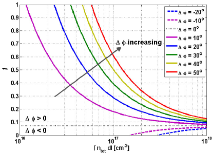
Figure 5: Contours of constant interferometer phase shift $\Delta\phi$ as a function of ionization fraction $f$ and line-integrated argon ion plus neutral density $\int n_{tot}{\rm d}l$, as calculated using Eq. (2).

where $f\equiv n_{i}/n_{tot}$ is the ionization fraction, $n_{tot}=n_{i}+n_{n}$ (where $n_{i}$ and $n_{n}$ are the ion and neutral densities, respectively), and the integral is over the chord path length. Note that $\Delta\phi<0$ when $f<0.07235$. Figure 5 shows selected contours of constant $\Delta\phi$, calculated using Eq. (2), as a function of $f$ and $\int n_{tot}{\rm d}l$.

III.3.2 Survey spectrometer

Spectrally resolved plasma self-emission is recorded with a survey spectrometer system consisting of a 5-mm diameter collimating lens (BK-7), a 19-element circular-to-linear silica-core fiber bundle (Fiberguide Industries “Superguide G,” 10 m long), a 0.275 m spectrometer (Acton Research Corp. SpectraPro 275) with three selectable gratings (150, 300, and 600 lines/mm), and a gated 1024-pixel multi-channel-plate array (EG&G Parc 1420). All measurements reported here were taken with the 600 lines/mm grating. We have taken measurements from about 300–900 nm, but all the data reported in this paper are between 430–520 nm. Two corrections are applied to the raw spectrum for each shot: (1) attenuation of the fiber bundle (approximately negative linear slope around -30 dB/km between 430–520 nm) and (2) pixel-dependent factor associated with the position of the grating in the spectrometer. The latter correction amplifies the spectra at low and high pixel-values over the raw spectrum by $\sim 1.7$–5 depending on the exact pixel value. We placed copper mesh in front of the collimating lens, as necessary, to keep the peak counts under about 16,000 to avoid saturating the detector. For the chord position which is $Z\approx 41$ from the railgun nozzle (see Fig. 4), the counts were of order 100, and thus no mesh was used. Before each shot day, a spectral lamp was used to record line emission at known wavelengths to provide a pixel-to-wavelength calibration. The spectral resolution for the data presented in this paper is 0.152 nm/pixel. The diameter of the viewing chord at the position of the jet, as imposed by the collimating lens, is approximately 7 cm, which constitutes a nominal spatial resolution for the spectroscopy data. The time resolution is 0.45 $\mu$s as determined by the exposure (gate) time of the detector. One spectrum at one time is taken for each shot.

III.3.3 Photodiode array

A three-channel photodiode array (PD1, PD2, and PD3) is used to collect broadband plasma emission for determining jet propagation speed. PD1, PD2, and PD3 collect light mostly transverse to the direction of jet propagation at $Z=2.7$, 27.7, and 52.7 cm, respectively (see Fig. 4). For each channel, light is collected through an adjustable aperture positioned in front of a collimating lens (Thorlabs F230SMA-B, 4.43 mm focal length), which is connected to a silica fiber that brings the light to the photodiode detectors inside a shielded enclosure. The silicon photodiodes (Thorlabs PDA36A) are amplified with variable gain, and have a wavelength range of approximately 300–850 nm. The peak responsivity is 0.65 A/W at 970 nm. The quoted frequency response decreases with increasing gain. For the data reported in this paper, the channels at $Z=2.7$, 27.7, and 52.7 cm had gain settings of 20, 50, and 50 dB, respectively, corresponding to quoted bandwidths of 2.1, 0.1, and 0.1 MHz. However, we note that the observed rise times for the second and third channels are much faster than the quoted 0.1 MHz bandwidth would dictate (see Sec. IV.1.1). All three channels had aperture openings of $<1$ cm, which constitutes a nominal spatial resolution for the photodiode data. The continuous (in time) photodiode signals are digitized at 40 MHz by the Joerger TR.

III.3.4 Fast-framing CCD camera

An intensified CCD camera (DiCam Pro ICCD), with spectral sensitivity from the UV to near-IR, is used to capture visible images of the plasma jet. The camera records $1280\times 1024$ pixel images with 12-bit dynamic range. The camera can record up to two images per shot. However, for inter-frame times below several tens of $\mu$s, the second image often has “ghosting” from the first frame. Thus, in this paper, we recorded only one frame per shot. The exposure (gate) is 20 ns. The camera is housed inside a metal shielding box and mounted next to a large rectangular borosilicate window on the vacuum chamber. A zoom lens (Sigma 70–300 mm 1:4–5.6) was used for recording the images shown in this paper. The camera is triggered remotely via an optical fiber. To infer quantitative spatial information from the CCD images, we recorded images with a meter stick held to the end of the railgun nozzle. Using these calibration images, we are able to determine pixel-to-centimeter conversion formulae (see Sec. IV.2.2). The CCD images presented in this paper are shown on a logarithmic scale in false color.

IV Experimental results

In this section, we present experimental results on the jet parameters (including velocity, density, temperature, and ionization fraction), structure, and evolution for the experimental data set spanning PLX shots 737–819.

IV.1 Jet parameters

IV.1.1 Velocity

The plasma jet velocity $V_{jet}$ is determined from photodiode array data and corroborated with interferometer data. The velocity is calculated by dividing the distance between viewing chords by the difference in arrival times of the peak signal. We use the arrival time of the peak signal rather than the leading edge to obtain a more robust estimate of the bulk jet velocity.

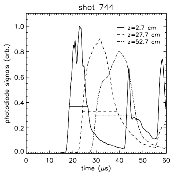
Figure 7: Photodiode array signals versus time. Horizontal lines denote the duration $\Delta t_{jet}$ over which the signals are greater than $1/e$ of the peak value (used in calculating jet length and rate of axial expansion). In this case, the velocities are 28.7 and 30.5 km/s between the first and second pairs of photodiodes, respectively. The $\Delta t_{jet}$ values are 7.9, 14.9, and 17.4 $\mu$s, and the jet lengths are 22.8, 44.2, and 53.0 cm at $Z=2.7$, 27.7, 52.7 cm, respectively.

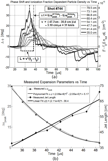
Figure 8: (a) Interferometer phase shifts versus time for all eight interferometer chords (distances $Z$ from the jet nozzle are indicated in the legend). Methodologies for calculating jet velocity and length are shown. (b) The peak phase shift $\Delta\phi_{peak}$ (squares) and jet length (diamonds) are shown for each chord at the time at which $\Delta\phi_{peak}$ for each chord occurs. Also shown are analytic fits to each set of data.

Figure 7 shows the three photodiode signals for a representative shot (744) from the data set analyzed in this paper. The signals are collected along viewing chords intersecting the jet propagation axis at distances $Z=2.7$, 27.7, and 52.7 cm, respectively, from the end of the gun nozzle (see Fig. 4). For this shot, the peak arrival times are 22.9, 31.6, and 39.8 $\mu$s, corresponding to average velocities of $V_{12}=28.7$ and $V_{23}=30.5$ km/s between the first and second pairs of photodiode viewing chords, respectively. For the entire data set considered in this paper, $V_{12}=28.9\pm 3.9$ km/s and $V_{23}=29.4\pm 4.5$ km/s, where the uncertainty is the standard deviation over the data set. The velocities did not vary significantly across this data set due to the relatively narrow range of peak gun current (255–285 kA) and total mass injected into the chamber (pressure rise 1.35–1.75 mTorr, corresponding to 31–40 mg of argon). A similar analysis using the interferometry data (see Fig. 8(a) for an example) from the chords at $Z=35.0$ and 47.7 cm yields an average jet velocity of $34.8\pm 5.6$ km/s (for the entire data set), which compares well with $V_{23}=29.4\pm 4.5$ km/s given above. The jet velocity appears to be nearly constant as it propagates over a nearly 50 cm distance. At 30 km/s, the jet $M=14$ (assuming that the jet is 100% argon, $\gamma=1.4$, $Z_{eff}=1$, and $T_{e}=1.4$ eV).

IV.1.2 Density, temperature, and ionization fraction

Plasma jet density $n$, electron temperature $T_{e}$, and ionization fraction $f$ are determined via a combination of experimental measurements and interpretation with the aid of theoretical analysis and atomic modeling. From spectroscopy, we determine electron density $n_{e}$ via Stark broadening of the impurity hydrogen H_β line (486.1 nm), and we estimate $T_{e}$ by comparing measured and calculated non-local-thermodynamic-equilibrium (non-LTE) argon spectra. Steady-state, collisional-radiation calculations with single-temperature Maxwellian electron distributions in the optically thin limit were performed using the PrismSPECT code with DCA (direct configuration accounting).MacFarlane et al. (2004) The following processes were included: electron-impact ionization, recombination, excitation, de-excitation, radiative recombination, spontaneous decay, dielectronic recombination, autoionization, and electron capture. The atomic model for argon consisted of 16,000 levels from all ionization stages with approximately 1500 over the lowest three ionization stages. The non-LTE calculations also provide the ionization fraction $f$ as a function of $n_{e}$ and $T_{e}$. The $f$ value is then used, in conjunction with Eq. (2) and the interferometer data, to provide an independent determination of $n_{tot}=n_{i}/f$. If we assume that $n_{e}=n_{i}$ (i.e., all ions are singly ionized, a reasonable assumption at our temperatures and densities), then $n_{e}=n_{i}=fn_{tot}$.

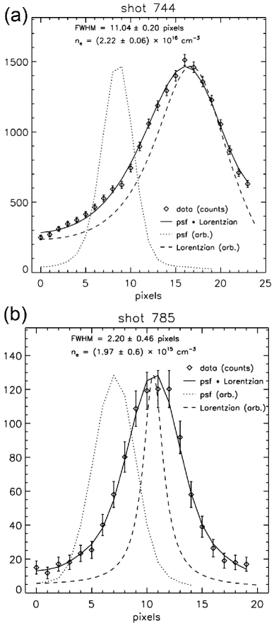
Figure 9: Determination of electron density $n_{e}$ via Stark broadening of the H_β line for shots (a) 744 ($t=17$ $\mu$s, nozzle view), and (b) 785 ($t=28$ $\mu$s, chord view). Shown are the experimental data (diamonds with error bars = $\pm\sqrt{\rm counts}$), an overlay of the measured instrumental broadening profile (dotted line, labeled as “psf” for point spread function), and a Lorentzian H_β profile (dashed line) that gives the best fit (minimum $\chi^{2}$) of the convolution (solid line) of the psf and the Lorentzian to the data. The $n_{e}$ is calculated from the Lorentzian full-width half-maximum (FWHM) using Eq. (3), and the uncertainty in $n_{e}$ is based on the standard deviation of the FWHM determined from curve-fitting.

Stark broadening of the H_β line is analyzed for the nozzle and chord views (see Fig. 4). The latter coincides with the position of the $Z=41.4$ cm interferometer chord. Figure 9 shows examples, from two shots (nozzle and chord views, respectively), of how $n_{e}$ is determined by fitting the convolution of the measured instrumental broadening (point spread function) and a Lorentzian profile to the experimentally measured H_β spectral feature. Curve-fitting is performed using the IDL (Interactive Data Language, http://www.exelisvis.com/IDL) routine curvefit. The $n_{e}$ is determined via

$$n_{e}~{}({\rm cm}^{-3})=2.53\times 10^{14}\left[\frac{\rm FWHM~{}(nm)}{\alpha_{1/2}}\right]^{3/2}=1.50\times 10^{13}\left[\frac{\rm FWHM~{}(pixels)}{\alpha_{1/2}}\right]^{3/2},$$ (3)

where FWHM is the full-width half-maximum of the Lorentzian fit, and $\alpha_{1/2}$ (in our case $=0.085$) is the so-called reduced half-width that scales as line shape and has been tabulatedStehlé and Hutcheon (1999) for many hydrogen lines for the temperature range 0.5–4 eV and density range $10^{14}$–$10^{18}$ cm^-3. The value of 0.152 nm/pixel for our spectrometer system has been used in Eq. (3). Table 1 summarizes our $n_{e}$ results obtained by Stark broadening analysis, and their corresponding viewing chords, times, and relative positions in the jet. The $n_{e}\approx 2\times 10^{16}$ cm^-3 near the gun nozzle falls by approximately one order of magnitude after the jet propagates approximately 41 cm. Unfortunately, the number of shots on which we could successfully perform the Stark broadening analysis was limited because the H_β line typically is obscured by a stronger nearby argon line. In the shots analyzed, the nearby argon line is subtracted out prior to performing Stark broadening analysis on the H_β line.

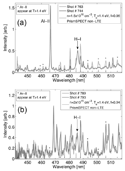
Figure 10: Intensity versus wavelength from the survey spectrometer with spectrometer views at the (a) nozzle ($t=17$ $\mu$s) and (b) chord ($t=36$ $\mu$s) positions. Shown in both plots are also the argon spectra of non-LTE PrismSPECT calculations with the parameters indicated in the respective legends. Appearance of the Ar ii lines in the data indicated by asterisks implies that peak $T_{e}\geq 1.4$ eV according to the PrismSPECT calculations.

Next, we use the spectroscopy results to obtain an estimate of $T_{e}$. Figure 10 shows spectrometer data for the (a) nozzle position at $t=17$ $\mu$s (corresponding to the rising edge of the jet) and (b) chord position at $t=36$ $\mu$s (corresponding to the jet bulk). The figure also shows calculated PrismSPECT non-LTE argon spectra for comparison. The Ar ii lines that appear in the experimental data only appear for $T_{e}\geq 1.4$ eV in the PrismSPECT non-LTE calculations, thus providing a lower bound estimate of the peak $T_{e}$ in the jet. The calculations show that $f=0.96$ (for $n_{e}=1.5\times 10^{16}$ cm^-3 and $T_{e}=1.4$ eV) and $f=0.94$ (for $n_{e}=2\times 10^{15}$ cm^-3 and $T_{e}=1.4$ eV) for the nozzle and chord positions, respectively. An upper bound on $T_{e}$ is also estimated based on the argon spectra centered around 794 nm (not shown). An Ar ii line visible in the calculations at $n_{e}=2\times 10^{16}$ cm^-3 and $T_{e}=1.7$ eV, but not visible in our measurements (shots 569-572 and 655-706), indicates an upper bound on the peak $T_{e}$ of 1.7 eV for the nozzle view. This upper bound also justifies our assumption that all argon ions are singly ionized. For the rest of the paper, we use $T_{e}=1.4$ eV, which is a more appropriate jet-averaged value, in estimating $T_{e}$-dependent quantities. Although $T_{i}$ has not been directly measured yet, it is reasonable for the purposes of this paper to assume that $T_{i}\approx T_{e}$ because the ion-electron thermal equilibration time $\bar{\nu}_{\epsilon}^{-1}=(3.2\times 10^{-9}Z_{eff}^{2}\ln\lambda n_{e}/\mu T^{3/2})^{-1}$, estimated to be 0.2 $\mu$s, is very fast compared to the jet evolution occurring over many tens of $\mu$s (where we have used $Z_{eff}=1$, $\ln\lambda=4.74$, $n_{e}=2\times 10^{16}$ cm^-3, $\mu=m_{i}/m_{p}=40$, and $T=1.4$ eV in estimating $\bar{\nu}_{\epsilon}$).

Finally, using the chord position $f=0.94$ determined above, an estimated interferometer chord path length $\approx 10$ cm at the $Z=41.4$ cm chord (see Sec. IV.2), and Eq. (2), we obtain an independent determination of $n_{e}=fn_{tot}$ from the interferometry data. The results are shown in Fig. 11, showing reasonable agreement in $n_{e}$ obtained via spectroscopy and interferometry. Table 2 summarizes all the experimentally measured jet parameters at both the nozzle and chord positions.

IV.1.3 Remark on the jet magnetic field

The evolution of the jet magnetic field $B$ after the jet exits the railgun has not been measured yet on PLX. The gun bore magnetic probes show that the field strength within the gun bore is on the order of several Tesla. The classical diffusion time of $B$ is approximately $\tau_{D}\sim\mu_{o}\delta^{2}/\eta_{\perp}$, where $\mu_{0}=4\pi\times 10^{7}$ H/m is the vacuum permeability, $\delta\approx 2$ cm the gradient scale length of $B$, and $\eta_{\perp}$ the perpendicular Spitzer resistivity. For $T_{e}=1.4$ eV, $n_{e}=2\times 10^{16}$ cm^-3, $Z_{eff}=1$, and $\ln\lambda=4.74$, $\eta_{\perp}=2.95\times 10^{-4}$ $\Omega$m and $\tau_{D}=1.7$ $\mu$s. Thus, for $V_{jet}\approx 3$ cm/$\mu$s, the magnetic field will decay to $e^{-3}=0.05$ of its original value after 5.1 $\mu$s or 15.3 cm of propagation. Assuming a value of 3 T in the gun bore, the decayed value after 5.1 $\mu$s will be 0.15 T, and the ratio of jet magnetic energy density $B^{2}/2\mu_{0}=9.0\times 10^{3}$ J/m³ to kinetic energy density $\rho V_{jet}^{2}/2=3.01\times 10^{5}$ J/m³ (assuming an argon density of $10^{16}$ cm^-3 and $V_{jet}=30$ km/s) will be about 0.03. Thus, it is reasonable to ignore (to leading order) the effects of the magnetic field on jet evolution over 0.5 m. We defer the direct measurement of jet magnetic field evolution to future work.

IV.2 Jet structure and evolution

In this sub-section, we present results on jet structure via CCD image, photodiode, and interferometer data, including quantitative results on jet length inferred from photodiode and interferometer data, and jet diameter inferred from CCD images and interferometer data. Note that our jets have a primary leading structure with several trailing structures, as seen in the $Z=2.7$ cm trace after $t=40$ $\mu$s in Fig. 7. By triggering a crowbar circuit to eliminate the ringing current (results not shown in this paper), we have successfully eliminated the trailing jet structures in both the photodiode and interferometer data. In this paper, we focus only on the properties of the leading jet structure in non-crowbarred shots.

IV.2.1 Jet length and axial profile

We estimate the jet length $L$ using the full-width at $1/e$ of the maximum of the photodiode (see Fig. 7 as an example) and interferometer (see Fig. 8(b) as an example) signals versus time to get a $\Delta t_{jet}$ for each photodiode and interferometer signal. It follows that $L\approx V_{jet}\Delta t_{jet}$, where $V_{jet}$ is determined by the difference in arrival times of the signal peaks, as described in Sec. IV.1.1. The photodiodes give $L_{1}=20.6\pm 3.5$ cm, $L_{2}=41.8\pm 4.4$ cm, and $L_{3}=48.9\pm 7.5$ cm (where the variation is the standard deviation over the data set) for the photodiode views at $Z=2.7$, 27.7, and 52.7 cm, respectively. The velocities used are $V_{12}=28.9$ km/s, $(V_{12}+V_{23})/2=29.1$ km/s, and $V_{23}=29.4$ km/s (see Sec. IV.1.1) for calculating $L_{1}$, $L_{2}$, and $L_{3}$, respectively. The interferometer chord at 41.4 cm, which is in between the photodiode views at $Z=25$ and 50 cm, gives $L_{int}=46.7\pm 6.5$ cm, consistent with $L_{2}<L_{int}<L_{3}$, where the velocity used is $34.8$ km/s.

The rate of jet length expansion $\dot{L}$ is determined from both the photodiode and interferometer data by taking $\Delta L/\Delta t$ between adjacent measurement positions. From the photodiode data over the entire data set, $\dot{L}_{12}=24.4\pm 5.4$ km/s and $\dot{L}_{23}=9.0\pm 7.3$ km/s, which correspond to the spatial ranges $Z=2.7$–27.7 cm and $Z=27.7$–52.7 cm, respectively. From the interferometer data, $\dot{L}_{int}=20.2\pm 14.0$ km/s for the spatial range $Z=35.0$–41.4 cm. If we assume $\dot{L}/2=2C_{s}/(\gamma-1)$ from hydrodynamic theory,Landau and Lifshitz (1987) where $C_{s}=9.79\times 10^{5}(\gamma Z_{eff}T_{e}/\mu)^{1/2}$, we get an independent estimate of $T_{e}=1.8$ eV (for $\dot{L}=\dot{L}_{12}=24.4$ km/s, $\mu=40$, $Z_{eff}=1$, and $\gamma=1.4$) that is in reasonable agreement with the range of $T_{e}=1.4$–1.7 eV determined in Sec. IV.1.2.

The jet axial profile can be inferred, qualitatively, from the photodiode and interferometer signals versus time. The time dimension can be converted approximately to a spatial dimension by multiplying by $V_{jet}\sim 30$ km/s or 3 cm/$\mu$s (which was done above to obtain $L=V_{jet}\Delta t_{jet}$). The qualitative jet axial profile as it comes out of the railgun is best observed in the $Z=2.7$ cm photodiode trace (Fig. 7), which shows a sharp rising edge lasting about 2 $\mu$s (6 cm). This is followed by some structure over about 5 $\mu$s (15 cm) and then by a falling tail that decays to about 10% of the peak intensity over about 10 $\mu$s (30 cm). Figure 11 gives a good representation of the jet axial profile farther downstream ($Z=41$ cm), based on interferometer density data.

For an average $V_{jet}=V_{12}=28.9$ km/s (see Sec. IV.1.1) as the jet exits the nozzle, this corresponds to an average $\Delta t_{jet}\approx L_{1}/V_{12}=7.1$ $\mu$s, which corresponds to the half-period of $I_{gun}$ (see Fig. 3). This suggests that the jet length is inversely proportional to the frequency of the pulsed-power railgun electrical circuit, and that the jet length can be tailored via electrical circuit parameters.

IV.2.2 Jet diameter and radial profile

The jet diameter $D$ is estimated by two methods. The first method is examining CCD image line-outs perpendicular to the jet propagation direction $Z$; this method also provides information regarding the jet radial profile. The second method uses the decay of the peak phase shift $\Delta\phi_{peak}$ of the eight interferometer chords and the assumption of conservation of total jet mass to deduce the jet diameter. We recognize that the two methods provide related but fundamentally different information, i.e., the first method relies on the intensity of emission from the jet plasma (which depends on both density and temperature) while the second method derives from the interferometer phase shift (which depends predominantly on the line-integrated plasma density). Nevertheless, the two methods give us meaningful quantitative estimates of the jet diameter and also provide qualitative information on the shape of the radial profile.

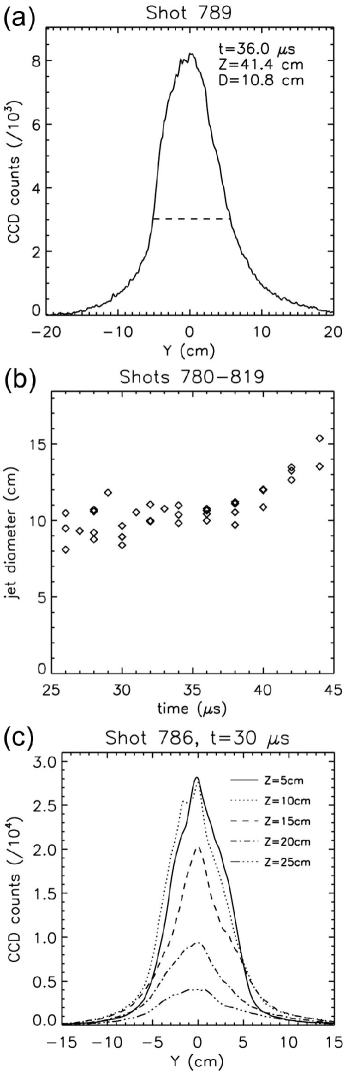
Figure 12: (a) CCD image line-out versus $Y$ (perpendicular to jet propagation direction) and the full-width (FW) at $1/e$ (dashed line) used to define the jet diameter $D$; (b) $D$ versus time at $Z=41.4$ cm from CCD line-outs (shots 780–819); (c) CCD line-outs at different $Z$ positions from a single shot, with FW at $1/e$ jet diameters of 8.2, 8.5, 8.5, 9.1, 10.6 cm for the increasing $Z$ values, respectively.

Figure 12(a) shows an example of a CCD image vertical line-out at $Z=41.4$ cm, and the estimate of $D$ based on the full-width at $1/e$ of the maximum. The time of this CCD image ($t=36.0$ $\mu$s) corresponds approximately to when the peak emission reaches $Z\approx 41$ cm (based on photodiode data). The line-out is taken after the CCD image is rotated slightly ($\approx 2^{\circ}$) such that the jet propagation axis is horizontal. The horizontal-pixel value ($x$) of the CCD image is converted to the $Z$ coordinate (cm) based on the formula $Z(x)=68.5-10^{5}x^{2}-0.041x$ (where $0<x<1023$). In addition, the cm/pixel conversion $\Delta Y$ in the vertical direction of the CCD image is obtained using the formula $\Delta Y(x)=2\times 10^{-5}x+0.041$ cm/pixel. The dependence of $\Delta Y$ on $x$ is due to the camera perspective, i.e., nearer objects appear larger in the image. These formulae were determined from a CCD image of a meter stick held to the end of the railgun nozzle. Figure 12(b) shows $D$ versus time at $Z=41.4$ cm determined using the full-width at $1/e$ method from a series of CCD images (shots 780–819). Note that $D$ determined via this method is fairly constant, with $D\sim 10$ cm from $t=26$–38 $\mu$s, but then $D$ increases after 38 $\mu$s, which corresponds to the time when the peak of the leading jet structure is passing through $Z=41$ cm (which can be deduced from Fig. 7). The expansion in $D$ at later times implies a lower $M$, suggesting that the trailing part of the jet is either hotter, slower, or both.

We also consider CCD image vertical line-outs at different $Z$ positions from a single shot at a single time ($t=30.0$ $\mu$s), as shown in Fig. 12(c). The diameters as determined by the full-width at $1/e$ of each peak are 8.2, 8.5, 8.5, 9.1, and 10.6 cm for $Z=5$, 10, 15, 20, and 25 cm, respectively. These emission line-outs provide information on the radial profile of the jet, and can provide further information on $n_{e}$ and $T_{e}$ profiles if compared with synthetic emission profiles generated using spectral modeling codes such as Spect3D.MacFarlane et al. (2007)

Next, we evaluate jet radial expansion using interferometer data. Figure 8(a) shows that $\Delta\phi_{peak}$ decreases with increasing $Z$ chord position. Figure 8(b) shows $\Delta\phi_{peak}$ versus time for each chord, and fits a quadratic function in time to the data points. From Eq. (2), it is apparent that $\Delta\phi_{peak}\sim n_{tot}D$ by assuming $\int n_{tot}{\rm d}l=n_{tot}D$ and constant $f$. By invoking conservation of total jet mass, we obtain the relationshipMerritt et al. (2012b)

$$n_{tot}(t)D(t)^{2}L(t)\sim\Delta\phi_{peak}(t)D(t)L(t)={\rm constant}\Rightarrow D(t)\propto\frac{1}{\Delta\phi_{peak}(t)L(t)},$$ (4)

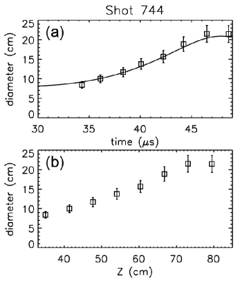
Figure 13: Plasma jet diameter versus (a) time and (b) $Z$, where the squares are from the data at each interferometer chord, and the solid line is from Eq. (4) using the fitting functions for $\Delta\phi_{peak}$ and $L$ given in Fig. 8(b). Error bars represent $\pm 10$% uncertainty in the determination of $L$, which is used in Eq. (4).

giving $D(t)$ in terms of experimentally measured quantities $\Delta\phi_{peak}(t)$ and $L(t)$, which are both shown in Fig. 8(b) for shot 744 as an example. By using the analytic fits to $\Delta\phi_{peak}(t)$ and $L(t)$ given in the legend of Fig. 8(b), it is straightforward to calculate $D(t)$ to within a constant that can be determined using $D(t=36~{}\mu{\rm s})\approx 10$ cm from Fig. 12(b). The result is shown in Fig. 13. Note that the diameter obtained at $Z\approx 41$ cm obtained from CCD image line-outs is likely an underestimate because the jet emission falls off more sharply than density if there is a peaked temperature profile. We regard the uncertainty of our reported diameter results based on CCD line-outs to be around a factor of two. The nominal radial expansion rate is $\approx 7$ km/s (between 36 and 43 $\mu$s), which is within the range $\dot{L}/2=10.1\pm 7.0$ km/s obtained between the interferometer chords at 35.0 and 41.4 cm.

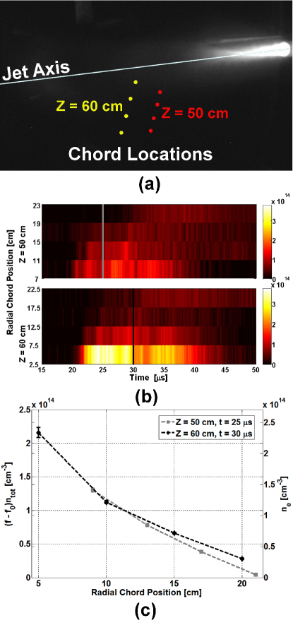
Figure 14: (a) Location of interferometer chords overlayed on the CCD image for shot 1106, on which we performed an Abel inversion analysis to obtain jet radial density profiles (for the yellow and red chord arrays separately). (b) Plots of $(f-f_{0})n_{tot}$ [cm^-3] versus radial chord position (relative to the jet axis) and time for the $Z\approx 50$ cm (top) and $Z\approx 60$ cm (bottom) chord positions; vertical lines indicate the times for which line-outs are shown next. (c) $(f-f_{0})n_{tot}$ and $n_{e}$ (data points) versus radial chord position at different times; $f=0.94$ and a maximum path length of 44 cm (corresponding to the path length of the innermost chord at $Z\approx 60$ cm) were used in calculating $n_{e}$. Error bars represent uncertainty in the chord positions of $\pm 0.5$ cm and also account for the slight variation in $Z$ of each chord array.

Finally, we show examples of the plasma jet radial density profiles deduced using Abel inversionHutchinson (2002) of two chord-arrays of interferometer data from a single shot (1106). This shot is not part of the data set analyzed in the rest of this paper because the Abel inversion analysis requires that the interferometer chords be arranged with different impact factors relative to the jet propagation axis $Z$, as shown in Fig. 14(a). For the main data set in this paper, the interferometer chords were arranged to intersect the $Z$ axis at different values of $Z$. Our Abel inversion analysis assumes cylindrical symmetry for the jet and four radially concentric zones of uniform density in each zone. The radii of the center of the zones correspond to the four interferometer chord positions (impact factors), respectively, for each $Z$ location, i.e., 5, 10, 15, and 20 cm for the $Z\approx 60$ cm chord array. The results of the Abel inversion are shown in Figs. 14(b) and 14(c), which show $(f-f_{0})n_{tot}$ and radial line-outs of $(f-f_{0})n_{tot}$ and $n_{e}$, respectively. From Fig. 14(c), it can be seen that the jet density profile is about a factor of two larger than the density profile from CCD image line-outs shown in Figs. 12(a) and 12(c).

V Conclusions and summary

The issues we address in this work (Sec. II.2) are determining the jet parameters, evaluating the evolution of the jet parameters as the jet propagates over about 0.5 m, and characterizing the jet axial and radial profiles to the extent possible. These issues are important for accurate assessments of the formation of imploding spherical plasma liners using merging plasma jets. The experimental data, while not in all cases definitive due to diagnostic limitations, offer crucial information about jet initial conditions and constraints on jet evolution that can enhance the accuracy of numerical modeling predictions.Loverich and Hakim (2010); Thoma et al. (2011); Cassibry et al. (2012); Cassibry, Stanic, and Hsu We reiterate that our plasma jet diagnostic measurements are all averaged over their viewing-chords, and therefore our reported results are mostly chord-averaged quantities.

We have presented results on jet parameters, summarized in Tables 1 and 2, showing that we are within a factor of 2–5 of what is needed to field the thirty-jet imploding plasma liner formation experiments specified in the PLX design.Hsu et al. (2012); Cassibry, Stanic, and Hsu Experiments at HyperV Technologies, using the same railgun design as the railgun used in this work but operating at $\gtrsim 500$ kA, have demonstrated the simultaneous achievement of the full PLX design parameters: density $\approx 10^{17}$ cm^-3, velocity $\approx 50$ km/s, and jet mass $\approx 8$ mg. Those results will be reported elsewhere. We operated at reduced railgun current ($\lesssim 300$ kA) in order to extend the railgun lifetime and maximize the amount of data collected. Although not emphasized in this paper, we have also learned how to operate the railgun reliably and taken note of where technological improvements should be made (mostly in the details of the pulsed-power system) for a thirty-gun experiment.

The need to understand the evolution of the jet as it travels a distance of about 0.5 m was a primary motivation for this work. To this end, our diagnostics were focused on two locations: the nozzle position right at the nozzle exit and the chord position about $Z=41$ cm away from the nozzle. The diagnostic views were transverse or mostly transverse to the jet propagation axis. We were able to determine that average $n_{e}$ fell by about one order of magnitude (from $2\times 10^{16}$ to $2\times 10^{15}$ cm^-3) over this distance, while average $T_{e}$ and $f$ remained nearly constant (within our measurement resolution). We were also able to determine the approximate jet length and diameter (see Table 2), and their evolution, showing that the jet volume increased by about one order of magnitude which is consistent with the drop in $n_{e}$. As discussed in Sec. II.2, the purely hydrodynamic prediction of constant-$M$ jet expansion has a large uncertainty due to a lack of precise knowledge of the exact expansion rate. This uncertainty is further exacerbated by the theory not accounting for radiative cooling which is expected to be important in our parameter regime. Using our measured jet parameters, the hydrodynamic theory predicts that the jet volume could increase by up to a factor of approximately 150. Our experimentally observed volume increase and density drop by about a factor of ten provides a useful constraint for validating numerical modeling results (that also include the effects of atomic physics) on jet propagation.

Adiabatic expansion of the jet would dictate that $nTV^{\gamma}={\rm constant}$. With a density drop of ten, a volume increase of ten, and $\gamma=1.4$, the average temperature should have dropped by a factor of about 2.5. The discrepancy between the latter and what was observed could potentially be explained by Ohmic heating associated with magnetic energy dissipation. The initial plasma jet thermal $\beta$ is $<0.01$, and thus the magnetic energy dissipation (discussed in Sec. IV.1.3) could easily balance thermal and radiative losses during jet propagation.

The radial and axial profiles of the jet are important variables for determining the dynamics of subsequent jet merging. The profiles are also needed for accurate numerical modeling of jet merging and plasma liner formation. We have assessed the radial and axial profiles to the extent possible via direct experimental measurements, and they are shown in Figs. 11, 12(a), 12(c), and 14(c). The profiles inferred from CCD image line-outs are dependent on both $n_{tot}$ and $T_{e}$, whereas the profiles inferred from interferometer data are dependent mostly on $n_{tot}$. If $T_{e}$ is peaked in both the radial and axial directions, as can be reasonably expected, then this means that the CCD line-outs will underestimate the width of the density profile. These profile data provide the opportunity to validate numerical modeling results by comparing the experimental profiles with synthetic data from post-processed numerical simulation results.

In summary, we have reported experimental results on the parameters, structure, and evolution of high-$M$ argon plasma jets launched by a pulsed-power-driven railgun. An array of thirty such jets has been proposed as a way to form imploding spherical plasma liners to reach 0.1–1 Mbar of stagnation pressure. Imploding plasma liners have potential applications as a standoff driver for MIF and for forming repetitive cm-, $\mu$s-, and Mbar-scale plasmas for HED scientific studies.

shot	view	time ($\mu$s)	position in jet	$n_{e}$ cm-3
744	nozzle	17	rising edge	$2.2\pm 0.1\times 10^{16}$
763	nozzle	17	rising edge	$1.6\pm 0.3\times 10^{16}$
738	nozzle	30	late in jet	$8.6\pm 0.0\times 10^{15}$
771	nozzle	35	late in jet	$5.8\pm 0.1\times 10^{15}$
785	chord	28	rising edge	$2.0\pm 0.6\times 10^{15}$
790	chord	38	just past peak	$2.0\pm 0.9\times 10^{15}$

Table 1: Summary of sight-line-averaged electron density determined via Stark broadening analysis of the H_β spectral line (486.1 nm). Nozzle view corresponds to just outside the railgun nozzle, and chord view corresponds to $Z\approx 41$ cm (see Fig. 4). The chord position results are also shown graphically in Fig. 11. The quoted uncertainties in $n_{e}$ are the standard deviations obtained from curve-fitting.

	nozzle ($Z\approx 2$ cm)	chord ($Z\approx 41$ cm)
$n_{e}$ (cm-3)	$2\times 10^{16}$	$2\times 10^{15}$
$T_{e}$ (eV)	1.4	1.4
$V$ (km/s)	30	30
$f$	0.96	0.94
$L$ (cm)	20	45
$D$ (cm)	5	10–20

Table 2: Summary of plasma jet parameters at the nozzle and chord positions, as determined by experimental measurements. The $n_{e}$ and $T_{e}$ values represent jet-averaged values.

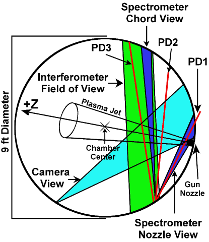
Figure 4: Diagnostic setup for the experiments reported in this paper. The spectrometer chord view corresponds to the $Z=41.4$ cm interferometer chord, and the spectrometer nozzle view is at the exit of the railgun nozzle. PD1, PD2, and PD3 are the three photodiode views.

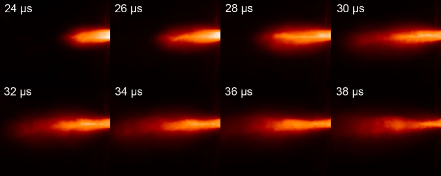
Figure 6: Plasma jet evolution as recorded by the CCD camera over 8 separate shots (800 and 784–790). The railgun nozzle is at the very right edge of each image. The images show the logarithm of the CCD intensity in false color.

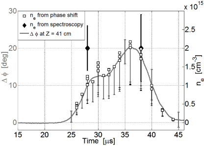
Figure 11: Interferometer phase shift $\Delta\phi$ averaged over shots 775–819 for the $Z=41.4$ cm chord (left hand y-axis) and electron density $n_{e}$ (right hand y-axis) versus time. The square data points are derived from Eq. (2) using $f=0.94$, interferometer $\Delta\phi$ data from the $Z=41.4$ cm chord, and the corresponding path length estimate based on the jet diameter $D$ obtained from CCD line-outs (discussed in Sec. IV.2.2). Error bars on the square data points represent uncertainty based on doubling the path length, which would halve the average $n_{e}$. The two diamond data points are from Stark broadening analysis of the H_β line from spectroscopy (shots 785 and 790). Each discrete data point corresponds to a separate shot.