B

a

Abstract

The viscoelastic material functions for the Becker and the Lomnitz rheological models, sometimes employed to describe the transient flow of rocks, are studied and compared. Their creep functions, which are known in a closed form, share a similar time dependence and asymptotic behavior. This is also found for the relaxation functions, obtained by solving numerically a Volterra equation of the second kind. We show that the two rheologies constitute a clear example of broadly similar creep and relaxation patterns associated with neatly distinct retardation spectra, for which analytical expressions are available.

FRACALMO PRE-PRINT:  http://www.fracalmo.org

 

2010 Physics and Astronomy Classification Scheme (PACS): 46.35.+z, 62.20.Hg, 76.60.-k, 83.60.Df, 91.32.-m

Key Words and Phrases: Linear viscoelasticity, rheology, creep, relaxation, retardation spectrum, Jeffreys-Lomnitz creep law, Becker creep law.

1 Introduction

The purpose of this paper is to draw the attention of polymer scientists on two models used in Earth rheology. They are usually refereed to as Becker and Lomnitz to honor the scientists who have introduced them in 1925 [1] and in 1956 [2], respectively. Both models exhibit slow varying creep laws suitable for simulating the flow and the (quasi frequency independent) energy dissipation in rocks, see e.g. Strick and Mainardi [3]. Though the corresponding relaxation laws are not considered in geophysical frameworks, they are certainly of interest in the theory and applications of linear viscoelasticty. As far as we know, in both classical and contemporary polymer science, see e.g. [4, 5, 6, 7], these rheological models have not been taken into account.

In the following we will discuss the analytical creep laws for the two models along with their graphical representation versus dimensionless time both in linear and logarithmic scales. Because the differences between the two creep laws remain small as time is evolving, we also show the rate of creep in order to have a better insight of the comparison. Then, we numerically compute and visualize the corresponding relaxation laws by solving a Volterra integral equation of the second kind. The major difference between the two models is found in their retardation spectra.

2 The creep laws

In Earth rheology, the law of creep is usually written as

$$J(t)=J_{U}[1+q\psi(t)]\,,\quad t\geq 0\,,$$

where $t$ is time, $J_{U}$ is the un-relaxed compliance, $q$ is a positive dimensionless material constant, and $\psi(t)$ is the dimensionless creep function. Consistently with the general theory of linear viscoelasticity, $\psi(t)$ is a Bernstein function, that is positive with a completely monotone derivative, with a related spectrum of retardation times (see e.g. Mainardi [8]).

For the Becker model [1] we have

$$\psi^{B}(t)=\hbox{Ein}(t/\tau_{0})\,,\quad t\geq 0\,,\quad\tau_{0}>0\,,$$

where Ein denotes the modified exponential integral function (see e.g. [8]). Assuming $\tau_{0}=1$, we have the integral and series representations

$$\hbox{Ein}(t)=\int_{0}^{t}\frac{\;1-\hbox{e}^{\displaystyle-u}}{u}\,du=\sum_{n=1}^{\infty}(-1)^{n-1}\frac{t^{n}}{n\,n!}\,,\quad t\geq 0\,,$$

hence the rate of creep is

$$\frac{d\psi^{B}}{dt}(t)=\frac{\;1-\hbox{e}^{\displaystyle-t}}{t}=\sum_{n=0}^{\infty}(-1)^{n}\frac{t^{n}}{(n+1)!}\,,\quad t\geq 0\ \,.$$

For the Lomnitz model [2] we have

$$\psi^{L}(t)=\hbox{log}(1+t/\tau_{0})\,,\quad t\geq 0\,,\quad\tau_{0}>0\,,$$

where log denotes the natural logarithmic function. Taking again $\tau_{0}=1$, we have the series representation

$$\hbox{log}(1+t)=\sum_{n=1}^{\infty}(-1)^{n-1}\frac{t^{n}}{n}\,,\quad t\geq 0\,,$$

which implies a rate of creep

$$\frac{d\psi^{L}}{dt}(t)=\frac{1}{1+t}=\sum_{n=0}^{\infty}(-1)^{n}{t^{n}}\,,\quad t\geq 0\,.$$

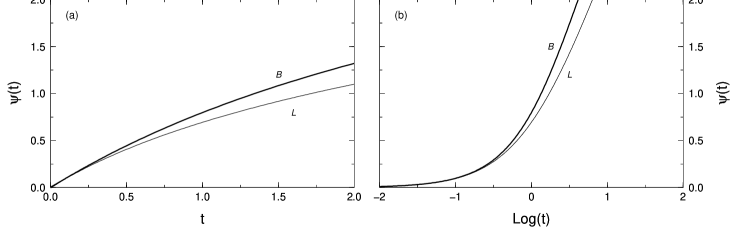
Figure 1: The creep functions for the Becker (B) and Lomnitz (L) rheologies, shown as a function of time.

For the Lomnitz law the series representations given by Eqs. (6) and (7) are convergent only for $0\leq t<1$, at variance with Eqs. (3) and (4) for the Becker law that are convergent for all $t\geq 0$. However, all these power series are suitable only for sufficiently small times because their numerical convergence falls down very soon.

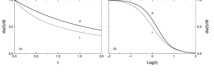
Figure 2: Rate of creep for the two models, as a function of time.

In order to compare the creep behavior of the two models, we show $\psi^{B}(t),\psi^{L}(t)$ and their time derivatives in Figures 1 and 2, respectively, taking both linear frame (a) and logarithmic (b) time axes. The overall similarity between the two creep functions is apparent in Figure 1, also showing that the Becker rheology accounts for a somewhat larger strain relative to Lomnitz (i.e., $\psi^{B}>\psi^{L}$). Inspection of the corresponding rates of creep in Figure 2, clearly shows that, for finite values of time, the Becker creep systematically evolves at a larger rate with respect to Lomnitz (i.e., $d\psi^{B}/dt>d\psi^{L}/dt$). For long times, both rates of creep decay to zero as $1/t$ as we easily note from Eqs. (4) and (7).

3 The relaxation laws

The relaxation modulus $G(t)$ for the two rheological models can be derived from the corresponding creep laws through the general Volterra integral equation of the second kind [8]

$$G(t)=\frac{1}{J_{U}}-\frac{1}{J_{U}}\,\int_{0}^{t}\frac{dJ(t^{\prime})}{dt^{\prime}}\,G(t-t^{\prime})\,dt^{\prime}\,.$$

As a consequence, the dimensionless relaxation function defined by

$$\phi(t)=J_{U}\,G(t)$$

obeys the integral equation

$$\phi(t)=1-q\,\int_{0}^{t}\,\frac{d\psi(t^{\prime})}{dt^{\prime}}\,\phi(t-t^{\prime})\,dt^{\prime}\,,$$

where the rate of creep is given by Eqs. (4) and (7) for the Becker and the Lomnitz laws, respectively. In order to solve numerically Eq. (10), we have used standard numerical methods.

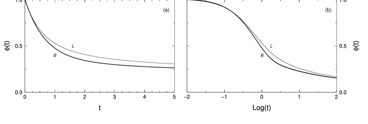
Figure 3: Relaxation functions for the two rheological bodies, as a function of time.

The results are shown in Figure 3, assuming $q=1$ and adopting again both linear and logarithmic time axes. As expected according to the similarity of the corresponding creep functions, the two relaxation functions show similar features for the two models. However, it is apparent that the Becker model exhibits, at a given time, a somewhat larger amount of relaxation relative to Lomnitz (i.e., $\phi^{B}<\phi^{L}$). By visual inspection of the curves it also appears that the Becker rate of relaxation exceeds that of Lomnitz model.

4 The retardation spectra

The determination of the time-spectral functions from the knowledge of the time-dependent material functions $J(t)$ and $G(t)$ is a fundamental problem from theoretical and experimental view points in polymer science. It can be formally solved through an analytical method outlined by Gross [9] based on the Laplace transform of the time derivatives of $J(t)$ and $G(t)$, see also [8]. For the present models we use the Gross method to derive the retardation spectrum from the Laplace transform of the rate of creep. By definition of the retardation spectrum $R_{\epsilon}(\tau)$, we have

$$J(t)=J_{U}+\displaystyle\int_{0}^{\infty}R_{\epsilon}(\tau)\,\left(1-\hbox{e}^{\displaystyle-t/\tau}\right)\,d\tau\,,$$

where $\tau$ denotes the retardation time.

For the two rheological models considered in this note, closed–forms exist for the retardation spectra. For the Becker model, according to [9], the retardation spectrum turns out to be discontinuous, with

$$R^{B}_{\epsilon}(\tau)={\frac{1}{\tau}}H(\tau-1)\,,$$

where $H(t)$ denotes the Heaviside step function, while from [10] for the Lomnitz model we have the continuous spectrum

$$R^{L}_{\epsilon}(\tau)=\frac{\hbox{e}^{\displaystyle-1/\tau}}{\tau}\,.$$

The two spectra are compared in Fig. 4 as function of $\tau$. Although these spectra show a dramatic difference character, we note that they both show a peak for $\tau=1$ and that they both decay, for $\tau\to\infty$, as $1/\tau$.

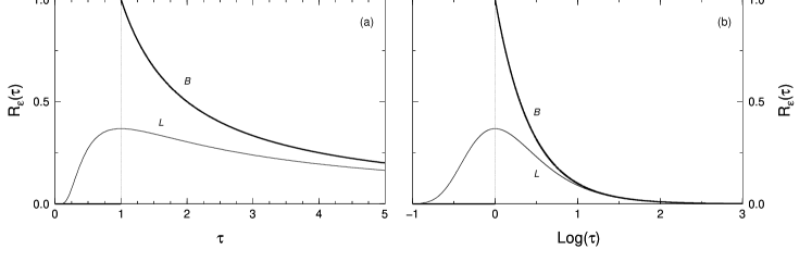
Figure 4: Retardation spectra for the two rheological models as a function of the retardation time.

5 Conclusions

In this paper we have discussed and compared the time-dependent material functions for two viscoelastic models introduced by Becker and Lomnitz known in Earth rheology. These functions for the two models show a broadly similar behavior, so that they could hardly be discriminated from experimental point of view. Despite this similarity, the corresponding retardation spectra show a dramatic difference. While the Lomnitz spectrum varies smoothly on the whole range of retardation times, the Becker one displays a cut off for short time even allowing a similar decay at large times. The examples discussed in this paper clearly show that in order to discriminate between two rheological models exhibiting very similar creep and relaxation behaviors the evaluation of the spectra is required.

References

- [1] R. Becker, Elastiche Nachwurking und Plastizität, Z. Phys. 33, 185–213 (1925).
- [2] C. Lomnitz, Creep measurements in igneous rocks, J. Geol. 64, 473–479 (1956).
- [3] E. Strick and F. Mainardi, On a general class of constant solids, Geophys. J. R. astr. Soc., 69, 415–429 (1982).
- [4] J.D. Ferry, Viscoelastic Properties of Polymers, Second edition Wiley, New York, 1980.
- [5] N.W. Tschoegel, The Phenomenological Theory of Linear Viscoelastic Behavior: an Introduction, Springer Verlag, Berlin, 1989.
- [6] L. Grassia and A. D’Amore, The relative placement of linear viscoelastic functions in amorphous glassy polymers, J. Rheology, 53 No 2, 339–356 (2009).
- [7] L. Grassia and A. D’Amore, On the interplay between viscoelasticy and structural relaxation in glassy amorphous polymers, J. Polymer Science. Part B: Polymer Physics, 47, 724–739 (2009).
- [8] F. Mainardi, Fractional Calculus and Waves in Linear Viscoelasticity, Imperial College Press–World Scientific, London, 2010.
- [9] B. Gross, Mathematical Structure of the Theories of Viscoelasticity, Hermann, Paris, 1953.
- [10] F. Mainardi and G. Spada, On the viscoelastic characterization of the Jeffreys-Lomnitz law of creep, Rheol. Acta, 51, 783–791 (2012). E-print: arXiv:1112.5543.