Non-Markovianity and Clauser-Horne-Shimony-Holt (CHSH)-Bell inequality violation in quantum dissipative systems

Abstract

We examine the non-Markovian dynamics in a multipartite system of two initially correlated atomic qubits, each located in a single-mode leaky cavity and interacting with its own bosonic reservoir. We show the dominance of non-Markovian features, as quantified by the difference in fidelity of the evolved system with its density matrix at an earlier time, in three specific two-qubit partitions associated with the cavity-cavity and atom-reservoir density matrices within the same subsystem, and the cavity-reservoir reduced matrix across the two subsystems. The non-Markovianity in the cavity-cavity subsystem is seen to be optimized in the vicinity of the exceptional point. The CHSH-Bell inequality computed for various two-qubit partitions show that high non-locality present in a specific subsystem appears in conjunction with enhanced non-Markovian dynamics in adjacent subsystems. This is in contrast to the matching existence of non-locality and quantum correlations in regions spanned by time $t$ and the cavity decay rate, $\lambda_{c}$ for select partitions. We discuss the applicability of these results to photosynthetic systems.

I Introduction

One of the most intriguing feature that underpins the many promising applications Niel of quantum theory is that it cannot be reduced to local realistic models in which the outcomes of local measurements are determined in advance by hidden variables bell . Non-locality which is linked to the violation of Bell inequality of any form, is considered to arise from complementarity or the impossibility of simultaneous joint measurements of observables. The Clauser-Horne-Shimony-Holt (CHSH) inequality chsh is the only extremal Bell inequality with two settings and two outcomes per site, and involves the comparison of predictions of quantum theories with theories rooted in local realism.

Entanglement and non-locality are distinct entities which are based on different frameworks. While entanglement is invariably linked to the mathematical formalism of the abstract Hilbert space, non-locality is founded on correlations of variables that, while amenable to experimental verification, has rather debatable origins due to the paradoxical, non-Boolean nature of quantum logic, with striking inconsistencies with the deterministic structures that underpins classical logic. The non-objectivity-non-locality issue invariably leads to inherent difficulties in formulating a rigorous definition of non-locality. Accordingly, the violation of any Bell inequality may imply the presence of non-locality, however a non violation does not guarantee the local or nonlocal nature of the correlations under study. Interestingly, the violation of a Bell inequality does not imply the existence of non-locality within the system where Bell test was performed, but it is a requirement william that non-locality is observed in the vicinity of the quantum system under observation. While non-locality is a feature which reflects entanglement, the converse is not true i.e., not all entangled states reveal non-local features. In other words, non-locality is a sufficient feature but not necessary to reveal entanglement busce .

A closely associated problem that has yet to be examined in depth is the role of non-divisible quantum maps, first proposed by Sudarshan $et$ $al$. sudar1 and examined in other related works Niel ; bre ; choi ; lind ; Kraus ; alicki ; sudar2 , on the violation of the CHSH inequality and the association between non-locality and non-Markovianity. The challenges of relating non-Markovian dynamics and maps that are not completely positive (CP) and which describe the evolution of open quantum systems is well known eis . The quantum Markov process as opposed to its non-Markovian counterpart is described by a subset of completely positive intermediate time dynamical maps usud , is limited by its strict applicability to weak system-environment interactions. In a dissipative environment, as is the case in this study, non-Hermitian effects are introduced and possibly a non-Markovian evolution involving some back flow of information to the system ensues. It would be interesting to examine non-Markovian processes of open quantum systems with non-divisible maps and which incorporate memory feedback mechanisms within the realm of non-locality. In a recent work lipra , the link between non-Markovian revivals and non-locality for a qubit-oscillator system was examined with results showing a strong correlation between revivals of non-locality and non-Markovian evolution dynamics of the studied system, nevertheless these trends were noted as not being indicative of a non-Markovian basis to changes during violation of the CHSH inequality. In an earlier work bella1 , the association between entanglement and non-locality was examined from a dynamical perspective, and closed relations were obtained for independent environments.

The main interest in non-Markovian processes arise from the fact that Markovian dynamics is typically only an approximation, which is no longer valid when considering shorter time-scales and/or stronger system-environment couplings as in light-harvesting systems where non-Markovianity appears significant under physiological conditions carupra ; reben . The non-Markovian measure has several interpretations with its evaluation based on a variety of physical measures depending on the evolution dynamics of the system under study. One popular computable measure was proposed by Breuer and coworkers breu2009 , where Markovianity is employed as a characteristic of the dynamical map $\rho(0)\mapsto\rho(t)=\Phi(t,0)\rho(0)$, and is associated with the decrease in the trace-distance which quantifies the distinguishability, $D[\rho_{1},\rho_{2}]$ between two system states, $\rho_{1},\ \rho_{2}$ . The distinguishability measure does not increase under all completely positive, trace preserving maps, hence $\sigma=dD[\rho_{1},\rho_{2},t]/dt$ is negative (positive) when information flows from (to) the system to (from) its environment. Consequently, the increase of trace distance during any time intervals is taken as a signature of the emergence of non-Markovianity over the period of dynamical evolution, and has been employed to examine dynamics of interactions in light-harvesting systems reben . The quantitative estimate of non-Markovianity is based on the cumulant of the positive information flux involving a maximization of all pairs of initial states to determine the largest amount of information that can be recovered from the environment breu2009 . Wolf $et$ $al$. wolf introduced an alternative measure of non-Markovianity based on divisibility, and subsequently Rivas $et$ $al$. Rivas2010 also proposed a measure of non-Markovianity based on deviations from divisibility and the characteristics of quantum correlations of the ancilla component of an entangled system evolving under a trace preserving completely positive quantum channel. The subject of equivalence of the two measures of non-Markovianity for open two-level systems has been topic of much interest in recent works hao ; chru , with the results indicating a dependence on the generic features of the quantum system for the two measures to be reconciled. It is to be noted that both measures are based on deviations from the continuous, memoryless, completely positive semi-group feature of Markovian evolution as is the case in other measures introduced recently.

Lu $et$ $al$. lu defined another measure of non-Markovianity using the quantum fisher information flow which quantifies the computable phase of the qubit undergoing decoherence due to its environment. Recently the fidelity of teleportation thilchem2 was seen to exhibit increased oscillation of fidelities in the non-Markovian regime of photosynthetic systems. Revivals of quantum correlations can exhibit revivals even in absence of back-action from the environment to the system, this feature was linked to the non-Markovian character of the map using a suitable quantifier of non-Markovianity in Ref. bella2 . Rajagopal and coworkers raja have explored the generality of the Kraus representation for both the Markovian and non-Markovian quantum evolution, highlighting the role of the fidelity measure $F[\rho(t),\rho(t+\tau)]$ Fidelity as being able to track salient properties of an evolved density matrix $\rho(t+\tau)$ as compared to a reference density matrix $\rho(t)$. This direct approach offers convenience in gauging non-Markovian signatures based on the fidelity difference $F[\rho(t),\rho(t+\tau)]-F[\rho(0),\rho(\tau)]$.

Our aim is twofold: (a) to examine the general relationships between non-Markovianity, non-locality and non-classical correlations zu in a multipartite system consisting of a qubit interacting with a structured reservoir in the form of a cavity in contact with its own reservoir. This multipartite arrangement provides different channels of decoherence and dissipation: one that occurs between the qubit and cavity and the second, between the cavity and reservoir, (b) to investigate the characteristic behavior of the entities in the vicinity of the exceptional points which are topological defects Heiss , which occur when two eigenvalues of an operator coalesce when selected system parameters are altered. As a result, two mutually orthogonal states merge into one self-orthogonal state, resulting in a singularity in the spectrum Heiss . Using the qubit-cavity-reservoir multipartite arrangement, we seek to examine the links between non-Markovianity, violation of the CHSH-Bell inequality and non-classical correlations in regions governed by the system parameters within various two-qubit partitions.

This paper is organized as follows. In Section II we derive analytical expressions for the atom-cavity-reservoir model with cavity losses based on a phenomenological master equation and the quantum trajectory approach. In Section II.1, the entanglement dynamics of a multipartite system of two noninteracting subsystems, each consisting of the two-level atom coupled to the cavity which interacts with its reservoir source is examined, with expressions obtained for several bipartite two-qubit density matrices. In Section III, analytical expressions of fidelities for several two-qubit partitions near the exceptional point are provided. Analysis of qualitative features of non-Markovianity based on the fidelity difference measure of specific subsystem are analysed in Section IV. In Subsection IV.1, qualitative features of non-Markovianity of the cavity-cavity subsystem obtained in Section IV is compared with those obtained using the trace-distance difference measure. In Section V, we make observations based on the non-Markovian results in Section IV and results of non-locality computed using the CHSH-Bell inequality. In Section V.1, we compare results of Bell non-locality and non-classical correlations for given partitions, and discuss the applicability of the results obtained in this study to photosynthetic systems in Section VI. Finally, Section VII provides our summary and some conclusions.

II Atom-cavity-reservoir model with cavity losses

We consider a multipartite system of Hamiltonian $\hat{H}_{T}$ which consists of a two-level atom coupled to a single-mode leaky cavity $s$, which in turn is interacting with its own source of bosonic reservoir $r$ ($\hbar$=1)

$$\hat{H}_{T} = \hat{H}_{s}+\hat{H}_{r}+\hat{H}_{I}\,$$ (1)

$$\hat{H}_{s} = \omega_{0}\;\sigma_{+}\;\sigma_{-}+\omega_{c}\,a^{\dagger}a+V(\sigma_{-}\,a^{\dagger}+\sigma_{+}\,a)\,$$ (2)

$$\hat{H_{r}} = \sum_{k}\omega_{k}b^{\dagger}_{k}b_{k},\quad\hat{H_{I}}=\sum_{k=1}^{N}(\varphi_{k}\hat{a}\hat{b}_{k}^{{\dagger}}+\varphi_{k}^{*}\hat{b}_{k}\hat{a}^{{\dagger}}),$$ (3)

where $\omega_{0}$ is the atomic resonance frequency, $\sigma_{+}(\sigma_{-})$ denotes the raising (lowering) operator of the atom, and $\hat{a}$   $(\hat{a}^{{\dagger}})$ annihilates (creates) a photon with frequency $\omega_{c}$ in the cavity mode. The operator $\hat{b}_{k}$   $(\hat{b}^{{\dagger}}_{k})$ annihilates (creates) a photon with frequency $\omega_{k}$ in $k$-th mode of the reservoir. $V$ is the coupling constant between qubit and cavity and $\varphi_{k}$ is the linear coupling between the cavity and reservoir.

The density operator $\rho$ of the quantum system associated with the total Hamiltonian, $\hat{H}_{T}$ (Eq. (1)) is obtained using the generalized Liouville-von Neumann equation $\frac{d\rho}{dt}=-i{\cal L}\rho$, where ${\cal L}$ generates the map from the initial to final density operators via a Liouville superoperator $\Phi(t,0)$: $\rho(0)\mapsto\rho(t)=\Phi(t,0)\rho(0)$. For the simple reversible and non-dissipative situation, and one in which the state commences in an uncorrelated combination of the atom-cavity subsystem and reservoir, the reduced dynamics of the atom-cavity subsystem can be obtained in the Kraus representation, by taking the trace over the reservoir degrees of freedom

$$\rho(t)=\sum_{i}K_{i}(t)\rho(0)K_{i}^{\dagger}(t),$$ (4)

where the operators $K_{i}$ constitute the Hilbert space of the subsystem, with $\sum_{i}\,K_{i}^{\dagger}K_{i}=I$, and $I$ is the identity matrix. The map in Eq. (4) projects a density operator to another positive density operator, and hence is a positive map. The separation of the total quantum system into a subsystem of immediate interest, and the reservoir environment which is generally considered to be in thermal equilibrium forms the basis of Eq. (4). This is not the case in most practical situations when both the Liouville operator and the map $\Phi(t,0)$ (for negative $t$) are not well defined as the dynamical evolution of the quantum state of the total system (atom, cavity and reservoir degrees of freedom) becomes irreversible and dissipative in nature, making it cumbersome for realistic modelling of even the atom-cavity subsystem.

Using the projection-operator partitioning method proposed by Feshbach fesh , the total Hilbert space of $\hat{H}_{T}$ (Eq. (1)) is divided into two orthogonal subspaces generated by the projection operator, ${\cal P}$ and its complementary projection operator ${\cal Q}=1-{\cal P}$. This allows the convenient study of the subspace of interest (atom-cavity in our case) within the total quantum system specified in Eq. (1). For our system, ${\cal P}=\sigma_{+}\;\sigma_{-}+a^{\dagger}a$ and ${\cal Q}=\sum_{k}b^{\dagger}_{k}b_{k}$, such that ${\cal PQ}={\cal QP}$=0. This means that the operators of the atom-cavity subsystem and the reservoir subsystem (which acts as the dissipative source) commute. The density operator associated with the qubit-cavity system is obtained using

$$\rho_{s}(t)={\cal P}\;\rho{\cal P},$$ (5)

where $\rho$ on the RHS of Eq. (5) is the density operator of the total system. An excitation present in the two-level atom $a$ (cavity $c$) is denoted by $\left|1\right\rangle_{a}$ ($\left|1\right\rangle_{c}$), whilst $\left|0\right\rangle_{a}$ ($\left|0\right\rangle_{c}$) correspond to the ground state atom (vacuum state of the cavity). The subspace ${\cal P}$ is spanned by ($\left|1\right\rangle_{a},\left|0\right\rangle_{a},\left|1\right\rangle_{c},\left|0\right\rangle_{c}$) while ${\cal Q}$ is spanned by ($\left|\mathbf{0}\right\rangle_{r},\left|\mathbf{1}\right\rangle_{r}$). The reservoir state $\left|\mathbf{0}\right\rangle_{r}$=$\prod_{k}\left|0\right\rangle_{k}$ denotes the vacuum of the reservoir, however its ortho-complement state, $\left|\mathbf{1}\right\rangle_{r}$ needs further explanation. We note that other than evolving under the action of the Hamiltonian associated with the atom-cavity subsystem ($\hat{H_{s}}$, Eq. (2)), the reservoir states also evolve under the reservoir Hamiltonian, $\hat{H_{r}}$ in Eq. (3). Hence we define the collective state of the reservoir sink, $\left|\mathbf{1}\right\rangle_{r}$, as a series of superposed terms, consisting of the state with a single excitation, $\left|\mathbf{1}\right\rangle_{r_{i}}$= $\frac{1}{R_{0}}\sum_{k}\;\varphi_{k}|1_{k}\rangle_{r}$ where $R_{0}=\sqrt{\sum_{k}|\varphi_{k}|^{2}}$, and other states orthogonal to it, $\left|\mathbf{1}\right\rangle_{r_{i}}$ (i = 2,3…) as follows

$$\left|\mathbf{1}\right\rangle_{r}=\frac{1}{\chi_{t}}\sum_{i}N_{i}\;\left|\mathbf{1}\right\rangle_{r_{i}}$$ (6)

where $\chi_{t}$ is the probability amplitude associated with the existence of an excitation in the collective reservoir state, with the atom and cavity, both remaining in the zero state. $|1_{k}\rangle_{r}$ denotes an excited oscillator in the $k$-th reservoir mode, with oscillators in all other modes remaining in the unexcited state.

Instead of a full microscopic derivation of the system dynamics associated with the Hamiltonian, $\hat{H}_{T}$ (Eq. (1)), we incorporate cavity losses by means of a phenomenological master equation which provides reliable results when the spectrum of the reservoir is approximately flat, as justified in a recent work scala which compared this model and a microscopic system-reservoir interaction model. The phenomenological master equation involving the reduced density matrix, $\rho_{s}$ appear as

$$\frac{\mathrm{d}}{\mathrm{d}t}\rho_{s}=i(\rho_{s}\;H_{s}-H_{s}\;\rho_{s})+\frac{\lambda_{a}}{2}(2\sigma_{-}\rho_{S}\sigma_{+}-\sigma_{+}\sigma_{-}\rho_{s}-\rho_{s}\sigma_{+}\sigma_{-})+\frac{\lambda_{c}}{2}(2a\rho_{s}a^{\dagger}-a^{\dagger}a\rho_{s}-\rho_{s}a^{\dagger}a),$$ (7)

where $\lambda_{a}$ ($\lambda_{c}$ )represents the atomic (cavity) decay rate. The master equation in Eq. (7) can be further simplified (setting $\lambda_{a}$=0) as follows

$$\frac{\mathrm{d}}{\mathrm{d}t}\rho_{s} = i(\rho_{s}\;H^{\prime}_{s}-H^{\prime}_{s}\;\rho_{s})+\lambda_{c}a\rho_{s}a^{\dagger},$$ (8)

$$H^{\prime}_{s} = H_{s}\;-\;i\frac{\lambda_{c}}{2}\;a^{\dagger}a$$ (9)

where the second term in the Hamiltonian $H^{\prime}_{s}$ constitutes a decay component which contributes to the non-Hermitian features in the system. The last term in Eq. (8) denotes the action of the jump operator which forms the basis of the quantum trajectory approach traj1 ; traj2 ; traj3 ; traj . In this approach, incoherent processes associated with non-Hermitian terms are incorporated as random quantum jumps which results in the collapse of the wavefunction. The net effect is the transfer of states from one subspace to the other, ${\cal P}\rightarrow{\cal Q}$. The density operator is obtained by taking an ensemble average of a range of conditioned operators traj1 at the select time $t$. It is important to note that while Eq. (8) describing the dynamics of the atom-cavity system is Markovian within one subspace, non-Markovian dynamics may arise in the interaction between the atom (cavity) and reservoir in different subspaces.

In order to obtain analytical solutions, we rewrite $H^{\prime}_{s}$ in Eq. (9) (c.f. $\hat{H_{s}}$, Eq. (2)) as

$$H^{\prime}_{s} = \omega_{0}\;\sigma_{+}\;\sigma_{-}+(\omega_{c}+\;\delta-\;i\frac{\lambda_{c}}{2})a^{\dagger}a+V(\sigma_{-}\,a^{\dagger}+\sigma_{+}\,a)\,,$$ (11)

$$\delta-\;i\frac{\lambda_{c}}{2}=\int\frac{|\varphi_{k}|^{2}}{\omega-\omega_{k}}g(\omega_{k})d\omega_{k}$$

where $\delta$ arises due to renormalization and energy integration is based on the assumption that the reservoir state energies are closely spaced. We intentionally ignore detailed parameters, such as spectral density and temperature, of the reservoir system for simplicity in analysis of the model under study. These boson bath parameters invariably determine the decay rate $\lambda_{c}$ as is obvious in Eq. (8). Moreover information related to the distribution of the phonon bath frequency including the cutoff frequency will influence the bath memory time, and accordingly the decay rate $\lambda_{c}$ incorporates leakages between subspaces. The latter processes are expected to result in a complicated mix of the distinct subspaces of ${\cal P}$ and ${\cal Q}$, with bearings on non-trivial non-Markovian dynamics between two subsystems present in the Hilbert space of $\hat{H}_{T}$ (Eq. (1)), this will be revealed in forthcoming Sections.

Considering the resonant condition $\omega_{0}=\omega_{c}+\delta$ and the presence of a single initial excitation in each subsystem, we write the multipartite state of the atom-cavity-reservoir as

$$\left|\psi_{t}\right\rangle=\left|1\right\rangle_{a}\otimes\left|0\right\rangle_{c}\otimes\left|\mathbf{0}\right\rangle_{r},$$ (12)

Following the quantum trajectory dynamics model traj1 , Eq. (12) evolves under the action of the Hamiltonian in Eq. (1) as follows

$$\left|\psi_{t}\right\rangle=\xi_{t}\left|1\right\rangle_{a}\left|0\right\rangle_{c}\left|\mathbf{0}\right\rangle_{r}+\eta_{t}\left|0\right\rangle_{a}\left|1\right\rangle_{c}\left|\mathbf{0}\right\rangle_{r}+\chi_{t}\left|0\right\rangle_{t}\left|0\right\rangle_{c}\left|\mathbf{1}\right\rangle_{r},$$ (13)

where $|\xi_{t}|^{2}$ ($|\eta_{t}|^{2}$) is the probability that the excitation is present in the atom (cavity). The probability amplitude, $\chi_{t}$, introduced earlier in Eq. (6) is evaluated using $|\chi_{t}|^{2}=1-|\xi_{t}|^{2}-|\eta_{t}|^{2}$.

For the initial condition, $\xi_{0}$=1, $\eta_{0}$=0, the analytical expressions for $\xi_{t}$ and $\eta_{t}$ can be obtained using

$$\frac{d\xi_{t}}{dt} = -iV\eta_{t}\,$$ (14)

$$\frac{d\eta_{t}}{dt} = -iV\xi_{t}-\frac{\lambda_{c}}{2}\eta_{t}\,$$

To simplify further analysis of the problem, we set $|\xi_{t}|^{2}=1-p$, $|\eta_{t}|^{2}=q$ and $|\chi_{t}|^{2}=p-q$. Here $q(t)$ is the probability of the atomic qubit exchanging quantum information with the cavity at time $t$, and $1-p(t)$ is the probability that the atomic qubit will remain in its excited state, provided it was in the excited state at $t=$0. The exchange mechanism obviously includes a dissipative measure, $\gamma_{d}$=$p$-$q$ which is non-zero in the event that the reservoir states coupled to the cavity gets excited. Accordingly, there exists a probability $p-q$ that the atomic qubit decays without exciting the cavity states, and we note that in the presence of non-Hermitian exchanges $p>q,\gamma_{d}>$0. In general $p(t)$ grows with time, and as will be shown later, it can incorporate feedback mechanisms associated with the non-Markovian dynamics of the multipartite state.

Eq. (14) yields the analytical forms for $p$, $q$ and appear as

$$p = 1-e^{-\lambda_{c}t/2}\left[\cos{\Omega}t+\frac{\lambda_{c}}{4\Omega}\sin{\Omega}t\right]^{2}$$ (15)

$$q = e^{-\lambda_{c}t/2}\frac{V^{2}}{\Omega^{2}}\sin^{2}{\Omega}t,$$ (16)

where the Rabi frequency $2\Omega=(4V^{2}-(\frac{\lambda_{c}}{2})^{2})^{1/2}$. Similar expressions as in Eq. (15) can be obtained via inversion of a Green’s function as detailed in an earlier work on the dissipative two-level dimer model thilaJCP . We note the existence of two regimes, depending on the relation between $V$ and $\lambda_{c}$. The range where $V>\frac{\lambda_{c}}{4}$ ($V<\frac{\lambda_{c}}{4}$) applies to the coherent (incoherent) tunneling regime, and at the exceptional point we obtain

$$\Omega=0,\;V=\frac{\lambda_{c}}{4}$$ (17)

At this point , both the coherent and incoherent tunneling regime merge and we obtain

$$p = 1-\left(1+\frac{\lambda_{c}t}{4}\right)^{2}e^{-\lambda_{c}t/2}$$ (18)

$$q = \left(\frac{\lambda_{c}t}{4}\right)^{2}e^{-\lambda_{c}t/2}$$ (19)

The exceptional point is a topological defect which is present in the vicinity of a level repulsion Heiss and unlike degenerate points, only one eigenfunction exists at the exceptional point due to the merging of two eigenvalues. The critical temperatures at which exceptional points occurs in photosynthetic systems was identified recently thilchem2 . In the restricted subspace subspaces of ${\cal P}$ occupied by the atom-cavity system, we note that the exceptional point in Eq. (17) may take on a range of values as the cavity decay rate, $\lambda_{c}$ is linked to almost continuous range of reservoir attributes.

II.1 Entanglement dynamics of a multipartite system incorporating non-Hermitian terms

Here we extend the composite system in Eqs.  (13) to examine the entanglement dynamics in a system of two noninteracting subsystems, each consisting of the two-level atom coupled to the cavity which interacts with its reservoir source. To simplify the analysis, we consider that the subsystems have identical environment with respect to their reservoir characteristics and cavity decay attributes, and assume a multipartite system in the initial state

$$\left|\Psi_{i}\right\rangle=\left(a\left|1_{a_{1}}0_{a_{2}}\right\rangle+b\left|0_{a_{1}}1_{a_{2}}\right\rangle\right)\left|0_{c_{1}}0_{c_{2}}\right\rangle\left|{{\bf 0}}_{r_{1}}{{\bf 0}}_{r_{2}}\right\rangle,$$ (20)

where $a,b$ are complex parameters, and the cavity $c$ and reservoir $r$ are present in their vacuum state. The two subsystems are labeled as $1$ or $2$.

The composite system, $\left|\Psi_{i}\right\rangle$ evolves as

$$a\left[\xi_{t}\left|1\right\rangle_{a_{1}}\left|0\right\rangle_{c_{1}}\left|{\bf 0}\right\rangle_{r_{1}}+\eta_{t}\left|0\right\rangle_{a_{1}}\left|1\right\rangle_{c_{1}}\left|{\bf 0}\right\rangle_{r_{1}}+\chi_{t}\left|0\right\rangle_{a_{1}}\left|0\right\rangle_{c_{1}}\left|{\bf 1}\right\rangle_{r_{1}}\right]\left|{0}_{a_{2}}{0}_{c_{2}}{\bf 0}_{r_{2}}\right\rangle$$ (21)

$$+b\left[\xi_{t}\left|1\right\rangle_{a_{2}}\left|0\right\rangle_{c_{2}}\left|{\bf 0}\right\rangle_{r_{2}}+\eta_{t}\left|0\right\rangle_{a_{2}}\left|1\right\rangle_{c_{2}}\left|{\bf 0}\right\rangle_{r_{2}}+\chi_{t}\left|0\right\rangle_{a_{2}}\left|0\right\rangle_{c_{2}}\left|{\bf 1}\right\rangle_{r_{2}}\right]\left|{0}_{a_{1}}{0}_{c_{1}}{{\bf 0}}_{r_{1}}\right\rangle$$ (22)

By tracing out the degrees of freedom of the qubits associated with the cavities $c_{1},c_{2}$, and reservoirs $r_{1},r_{2}$, the reduced density matrix of the bipartite two-qubit atomic system at time $t$ (as determined by $p,q$) is obtained in the basis $\{\left|00\right\rangle,\left|01\right\rangle,\left|10\right\rangle,\left|11\right\rangle\}$ as

$${\rho}_{a_{1},a_{2}}(t)=\left(\begin{array}[]{cccc}p&0&0&0\\ 0&|b|^{2}(1-p)&a^{\star}b\;(1-p)&0\\ 0&b^{\star}a\;(1-p)&|a|^{2}(1-p)&0\\ 0&0&0&0\\ \end{array}\right)\\$$ (23)

Likewise, by tracing out the degrees of freedom of the qubits associated with $a_{1},a_{2}$, and $r_{1},r_{2}$ ($c_{1},c_{2}$), the reduced density matrix of the remaining bipartite-equivalent partitions associated with the two-cavity (two-reservoir) system, ${\rho}_{c_{1},c_{2}}(t)$ (${\rho}_{r_{1},r_{2}}(t)$) can be obtained in the basis $\{\left|00\right\rangle,\left|01\right\rangle,\left|10\right\rangle,\left|11\right\rangle\}$ by the substitution $(1-p)\rightarrow q$ ($(1-p)\rightarrow\gamma_{d}$).

For the non-equivalent atom-cavity partition, we obtain an associated reduced density matrix (${\rho}_{a_{i},c_{i}}$) (i=1,2) within the same subsystem as follows

$${\rho}_{a_{i},c_{i}}(t)=\left(\begin{array}[]{cccc}|a|^{2}\gamma_{d}+b^{2}&0&0&0\\ 0&|a|^{2}q&|a|^{2}\sqrt{1-p}\sqrt{q}&0\\ 0&|a|^{2}\sqrt{1-p}\sqrt{q}&|a|^{2}(1-p)&0\\ 0&0&0&0\\ \end{array}\right)\\$$ (24)

Likewise the reduced density matrix (${\rho}_{a_{i},r_{i}}$) associated with the atom-reservoir partition is obtained as

$${\rho}_{a_{i},r_{i}}(t)=\left(\begin{array}[]{cccc}|a|^{2}q+b^{2}&0&0&0\\ 0&|a|^{2}\gamma_{d}&|a|^{2}\sqrt{1-p}\sqrt{\gamma_{d}}&0\\ 0&|a|^{2}\sqrt{1-p}\sqrt{\gamma_{d}}&|a|^{2}(1-p)&0\\ 0&0&0&0\\ \end{array}\right)\\$$ (25)

while the reduced density matrix (${\rho}_{c_{i},r_{i}}$) associated with the cavity-reservoir partition is obtained as

$${\rho}_{c_{i},r_{i}}(t)=\left(\begin{array}[]{cccc}|a|^{2}(1-p)+b^{2}&0&0&0\\ 0&|a|^{2}\;\gamma_{d}&|a|^{2}\sqrt{q}\sqrt{\gamma_{d}}&0\\ 0&|a|^{2}\sqrt{q}\sqrt{\gamma_{d}}&|a|^{2}q&0\\ 0&0&0&0\\ \end{array}\right)\\$$ (26)

The reduced matrices (${\rho}_{a_{1},r_{2}}$ ($i\neq j$) associated with the atom-reservoir partition across different subsystems is obtained as

$${\rho}_{a_{1},r_{2}}(t)=\left(\begin{array}[]{cccc}|a|^{2}(q+\gamma_{d})+|b|^{2}(1-\gamma_{d})&0&0&0\\ 0&|b|^{2}\;\gamma_{d}&a^{*}b\sqrt{\gamma_{d}(1-p)}&0\\ 0&ab^{*}\sqrt{\gamma_{d}(1-p)}&|a|^{2}(1-p)&0\\ 0&0&0&0\\ \end{array}\right)\\$$ (27)

The remaining inter-system partitions, ${\rho}_{a_{i},c_{j}}$, ${\rho}_{c_{i},r_{j}}$) ($i\neq j$), are expected to display entanglement dynamics and non-locality characteristics not distinctly different from those considered above, and therefore will be omitted from further consideration.

III Fidelity measure for two-qubit partitions

The fidelity measure $0\leq F[\rho(t),\rho(t^{\prime})]\leq 1$ quantifies the distance between the initial state $\rho(t)$ and the evolved state $\rho(t^{\prime})$ at a later time $t^{\prime}$ and is defined as Fidelity

$$F[\rho(t),\rho(t^{\prime})]=\left\{{\rm Tr}\left[\sqrt{\sqrt{\rho(t)}\rho(t^{\prime})\sqrt{\rho(t)}}\right]\right\}^{2},$$ (28)

and satisfies the symmetry property, $F[\rho(t),\rho(t^{\prime})]=F[\rho(t^{\prime}),\rho(t)]$. Based on this definition, the fidelity measure $\mathit{F}$ between the initial state at $t$=0 (for which $p,q,\gamma_{d}$=0) and which terminate as the state in Eqs.(23), (24), (25), (26) or (27) at a later time $t$ is obtained as

$$\mathit{F}_{1}\left({\rho}_{a_{1},a_{2}}(0),{\rho}_{a_{1},a_{2}}(t)\right) = 1-p,\quad\left[e^{-\frac{t\lambda_{c}}{2}}\left(1+\frac{t\lambda_{c}}{4}\right)^{2}\right].$$ (29)

$$\mathit{F}_{2}\left({\rho}_{c_{1},c_{2}}(0),{\rho}_{c_{1},c_{2}}(t)\right) = 1-q,\quad\left[1-\frac{1}{16}e^{-\frac{t\lambda_{c}}{2}}t^{2}\lambda_{c}^{2}\right].$$

$$\mathit{F}_{3}\left({\rho}_{r_{1},r_{2}}(0),{\rho}_{r_{1},r_{2}}(t)\right) = 1-\gamma_{d},\quad\left[\frac{1}{8}e^{-\frac{t\lambda_{c}}{2}}(8+(t\lambda_{c})^{2}+4t\lambda_{c})\right].$$

$$\mathit{F}_{4}\left({\rho}_{a_{1},c_{1}}(0),{\rho}_{a_{1},c_{1}}(t)\right) = \left(\sqrt{a^{4}(1-p)}+\sqrt{b^{4}+a^{2}b^{2}\gamma_{d}}\right)^{2},\quad\left[\frac{1}{16}\left(\sqrt{a^{4}e^{-\frac{t\lambda_{c}}{2}}(t\lambda_{c}+4)^{2}}+4\sqrt{b^{2}-\frac{1}{8}a^{2}b^{2}e^{-\frac{t\lambda_{c}}{2}}(8+(t\lambda_{c})^{2}+4t\lambda_{c})}\right)^{2}\right].$$

$$\mathit{F}_{5}\left({\rho}_{a_{1},r_{1}}(0),{\rho}_{a_{1},r_{1}}(t)\right) = \left(\sqrt{a^{4}(1-p)}+\sqrt{b^{4}+a^{2}b^{2}q}\right)^{2},\quad\left[\left(\sqrt{a^{4}e^{-\frac{t\lambda_{c}}{2}}\left(1+\frac{t\lambda_{c}}{4}\right)^{2}}+\sqrt{b^{4}+\frac{1}{16}a^{2}e^{-\frac{t\lambda_{c}}{2}}t^{2}\lambda_{c}^{2}b^{2}}\right)^{2}\right].$$

$$\mathit{F}_{6}\left({\rho}_{c_{1},r_{1}}(0),{\rho}_{c_{1},r_{1}}(t)\right) = b^{2}+a^{2}(1-p),\quad\left[b^{2}+a^{2}e^{-\frac{t\lambda_{c}}{2}}\left(1+\frac{t\lambda_{c}}{4}\right)^{2}\right].$$

where the corresponding fidelities near the vicinity of the exceptional point are provided within the square brackets.

The fidelities $\mathit{F}_{i}$ (i=1 to 6) between various subsystems for $\lambda_{c}<$4, are shown in Fig. 1. At the exceptional point (setting $\hbar=V=$1), $\lambda_{c}$=4, and minimum passage time $t$=1, $p$=1. We note that the fidelity of the cavity-cavity partition experiences a minimum at $t$=1, which appears to be a characteristic feature of the cavity-cavity subsystem acting as a quantum channel. The local minimum in the fidelity measure may be linked to the merging of two eigenvalues at the exceptional point Heiss and a corresponding loss of distinguishability. As expected, fidelities of all other subsystem decrease with time, and in particular the loss in fidelities of the atom-atom and reservoir-reservoir subsystems are almost similar. The decrease in fidelity of the reservoir-reservoir subsystem without any revival, is consistent with the role of a dissipative sink as there is a one-directional information flow between subspaces of ${\cal P}$ and ${\cal Q}$, and the dissipative measure, $\gamma_{d}$ increases with time. This feature is expected to be present in photosynthetic sinks as well.

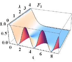
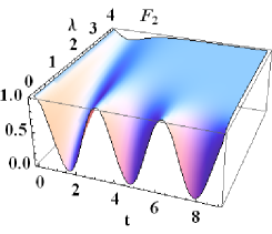
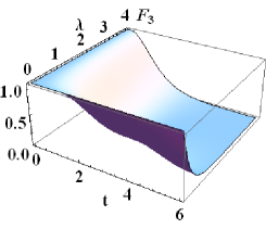
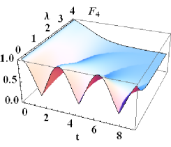
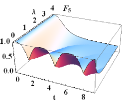
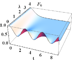
Figure 1: Fidelities $\mathit{F}_{i}$ (i =1..6) between various subsystem partitions as a function of dimensionless time $t$ and decay rate $\lambda_{c}$. $\mathit{F}_{1}\equiv$ atom-atom partition, $\mathit{F}_{2}\equiv$ cavity-cavity partition, $\mathit{F}_{3}\equiv$ reservoir-reservoir partition, $\mathit{F}_{4}\equiv$ atom-cavity partition, $\mathit{F}_{5}\equiv$ atom-reservoir partition, $\mathit{F}_{6}\equiv$ cavity-reservoir partition. The unit system adopted here and in all other figures is based on $\hbar=V=$1, with time $t$ obtained as inverse of $\Omega_{0}$ (at $\lambda_{c}$ = 0)

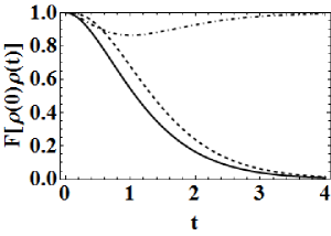
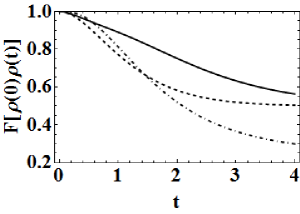
Figure 2: Fidelities $\mathit{F}_{i}$ (i =1..6) of various subsystem partitions as a function of dimensionless time $t$ at the vicinity of the exceptional point. Solid lines ($\mathit{F}_{1}$, $\mathit{F}_{4}$), DotDashed ($\mathit{F}_{2}$, $\mathit{F}_{5}$), Dashed ($\mathit{F}_{3}$, $\mathit{F}_{6}$)

IV Non-Markovianity based on the Fidelity measure

For a system density matrix undergoing Markovian evolution under completely positive, trace preserving dynamical maps $\Phi$, the fidelity measure $F[\rho(t),\rho(t+\tau)]$ between the initial state $\rho(t)$ and the evolved state $\rho(t+\tau)$ at a later time $t+\tau$. satisfies raja

$$F[\rho(t),\rho(t+\tau)]\equiv F[\Phi(t)\rho(0),\Phi(t)\rho(\tau)]$$

$$\Rightarrow F[\rho(t),\rho(t+\tau)]\geq F[\rho(0),\rho(\tau)].$$ (30)

The violation of the inequality in Eq. (IV) was proposed as a signature of non-Markovian dynamics by Rajagopal et. al. raja . Accordingly negative values of the following fidelity difference function

$$G(t,\tau)=\frac{F[\rho(t),\rho(t+\tau)]-F[\rho(0),\rho(\tau)]}{F[\rho(0),\rho(\tau)]},$$ (31)

are correlated with non-Markovianity during the evolution dynamics of the quantum state. Using the two-qubit matrices which appear in Eqs.(23), (24), (24), (25) and the expressions for $p$ and $q$ in Eqs.(15), (16), the fidelity difference function $G(t,\tau)$ can be evaluated as analytical expressions of $t,\tau$ and $\lambda_{c}$. Due to the lengthy expressions for these functions, we only provide numerical results which show subtle changes of $G(t,\tau)$ with $\lambda_{c}$ for the various subsystems.

Fig. 3 illustrates the fidelity difference $G(t,\tau)$ as a function of $t$ and $\tau$ for the reduced density matrix corresponding to the atom-reservoir subsystem (Eq.(25)) for increasing $\lambda_{c}$. The sensitivity of the two-qubit dynamics on $\tau$ translates in a striking way to the non-Markovianity measure, with the qubit dynamics becoming Markovian beyond a critical damping $\lambda_{c}$, and as expected depends on the initial correlation amplitude factors, $a,b$. At $\lambda_{c}$=0, the oscillatory state of information exchanges between the atomic qubit and reservoir is captured by the symmetric pattern of non-Markovian dynamics alternating with Markovian dynamics. The non-Markovianity decreases with higher values of the cavity decay rate $\lambda_{c}$, consistent with decreased population transfer between the atom-cavity subsystem. Specifically, we note the persistence of non-Markovianity at small $t,\tau$ values, even at higher values of the cavity decay rate $\lambda_{c}\approx$ 5.

As expected, there is insignificant non-Markovian signatures seen in a atom-cavity partition within the same subsystem. In contrast to the lack of non-Markovianity in the atom-cavity partition , we noted richness in non-Markovian dynamics for the atom-reservoir (${\rho}_{a_{1},r_{2}}$ ($i\neq j$) partition across different subsystems, and similar to that shown in Fig. 3. In this case, the two-qubit dynamics becomes fully Markovian at a smaller critical damping if a small initial correlation amplitude factor, $a$ is used.

The fidelity difference $G(t,\tau)$ is also seen to undergo notable changes (with $t$ and $\tau$) in the case of the reduced density matrix corresponding to the cavity-cavity subsystem ( Eq.(23) with the substitution $(1-p)\rightarrow q$), as shown in Fig. 4. Here, the non-Markovianity appear to be enhanced in some regions as the cavity decay rate $\lambda_{c}$ is increased. In the vicinity of the exceptional point, we note a transition in which regions of non-Markovianity merge, and Markovian processes are eliminated. The exceptional point appear to signal the enhancement of non-Markovianity in selected regions (of time $t$ and $\lambda_{c}$) for the cavity-cavity partition.

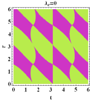
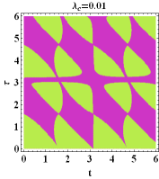
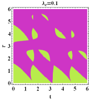
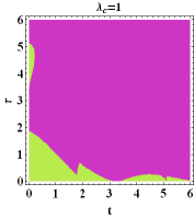
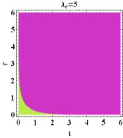
Figure 3: Fidelity difference $G(t,\tau)$ as a function of $t$ and $\tau$ for the reduced density matrix corresponding to the atom-reservoir subsystem (Eq.(25)), and increasing $\lambda_{c}$. $a$=$b$=$\frac{1}{\sqrt{2}}$. Non-Markovian trends were not significant for the intra-system atom-cavity and cavity-reservoir partitions. Negative values indicating non-Markovianity are shaded green, while regions which are shaded purple imply non-violation of the inequality (IV) and hence Markovian evolution dynamics. Non-Markovianity decreases with higher values of the cavity decay rate $\lambda_{c}$.

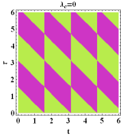
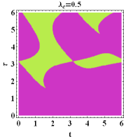
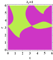
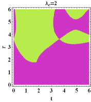
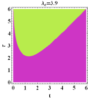
Figure 4: Fidelity difference $G(t,\tau)$ as a function of $t$ and $\tau$ for the reduced density matrix corresponding to the cavity-cavity subsystem ( Eq.(23) with the substitution $(1-p)\rightarrow q$). $a$=$b$=$\frac{1}{\sqrt{2}}$. Colour codes follows as specified in Fig. 3. Unlike Fig. 3, non-Markovianity continue to persist for higher values of the cavity decay rate $\lambda_{c}$ in some regions.

IV.1 Non-Markovianity based on other distance measures

It may be worthwhile to examine other physical quantities, which are functions of the dynamical map, that describe the open system evolution of the physical states. In an earlier work usud , the use of relative entropy difference to qualitatively capture the departure from the completely positive Markovian semigroup property of evolution was verified to assume negative values under an open system non-completely positive dynamics. We recall that the relative entropy veple of two density matrices $\rho$ and $\gamma$, defined by: $S(\rho||\gamma)={\rm Tr}[\rho(\ln\rho-\ln\gamma)]$ is positive and vanishes if and only if $\rho\equiv\gamma$. Under completely positive, trace preserving dynamical maps $\Phi$, the relative entropy obeys monotonicity property which yields a relation which is analogous to Eq.(IV)

$$S[\rho(t)||\rho(t+\tau)] \equiv S[\Phi(t)\rho(0)||\Phi(t)\rho(\tau)]$$ (32)

$$\leq S[\rho(0)||\rho(\tau)]$$

The relative entropy difference $S(t,\tau)$ given by

$$S(t,\tau)=\frac{S[\rho(0)||\rho(\tau)]-S[\rho(t)||\rho(t+\tau)]}{S[\rho(0)||\rho(\tau)]}$$ (33)

is necessarily positive for all quantum states $\rho(t)$ evolving under completely positive Markovian dynamics and violation of the inequality in Eq.(32) i.e., $S(t,\tau)<0$, denotes the occurrence of non-Markovian dynamical processes in the quantum system under study.

Similar to the relative entropy difference, the trace-distance $D[\rho_{1},\rho_{2}]=\frac{1}{2}||\rho_{1}-\rho_{2}||$ Niel where $||A||=Tr[\sqrt{A^{\dagger}A}]$ between $\rho_{1},\ \rho_{2}$, can be used to define the trace-distance difference

$$D(t,\tau)=\frac{D[\rho(0),\rho(\tau)-D[\rho(t),\rho(t+\tau)]}{D[\rho(0),\rho(\tau)]},$$ (34)

and to identify violation of the monotonically contractive characteristic feature associated with divisible Markovian mapping on the operator space. We note that both the relative entropy and trace-distance decline during a complete positive Markovian process, unlike the fidelity which increases under the same conditions. As pointed out earlier in Ref. usud , negative values of relative entropy difference (33) and the fidelity difference (31) only imply that the time evolution is not a completely positive Markovian process, positive values of these same quantities does not imply the occurrence of a Markovian evolution. Accordingly, the negative values of relative entropy and fidelity differences serve as sufficient but not necessary signatures of non-Markovianity (completely positive as well as non-completely positive). In order to highlight the latter point, we have repeated the calculations of the fidelity difference $G(t,\tau)$ (Eq.(31)) as a function of $t,\tau$ done earlier, by using the trace-distance difference $D(t,\tau)$ (Eq.(34) for the cavity-cavity two-qubit partition ( Eq.(23) with the substitution $(1-p)\rightarrow q$), and illustrated in Fig. 5.

Comparing the results of Fig. 4 and Fig. 5, we note that non-Markovianity is optimized in the vicinity of the exceptional point in both cases, however there are subtle differences.The trace-distance difference measure yields enhanced features in that it is able to detect the presence of non-Markovianity at small $\tau$ which remains undetected by the fidelity difference measure. Similar trends have been noted usud with the relative entropy difference, which shows the dependence of non-Markovianity dynamics on the metric entity. It appears that regions of contractive quantum evolution vary according to the measure used to detect violations of Markovian dynamics. In general one can conclude (at least on the basis of the results obtained in this study) that these differences are marginal and there is overall agreement in the critical regions of non-Markovianity. In the next Section, we make several important observations based on the non-Markovian patterns of Figs. 3, 4 and 5 and results of non-locality computed using the CHSH-Bell inequality.

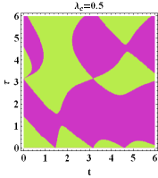
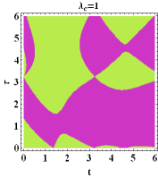
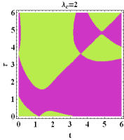
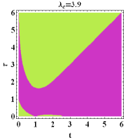
Figure 5: Trace difference $D(t,\tau)$ (Eq.(34) as a function of $t$ and $\tau$ for the reduced density matrix corresponding to the cavity-cavity subsystem ( Eq.(23) with the substitution $(1-p)\rightarrow q$). $a$=$b$=$\frac{1}{\sqrt{2}}$. Colour codes follows as specified in Fig. 3. Unlike Fig. 4, non-Markovianity appear to be present at small $\tau,t$ that remains undetected by the fidelity difference measure. In any case, there is overall agreement with Fig. 4 in that non-Markovianity is optimized in the vicinity of the exceptional point.

V Violation of the CHSH-Bell inequality

The violation of the Bell inequality $|\mathcal{B}|\leq 2$ is quantified by the CHSH- Bell inequality function $\mathcal{B}$ of a two-qubit density matrix where $\mathcal{B}=M(\vec{a},\vec{b})-M(\vec{a},\vec{b}^{\prime})+M(\vec{a}^{\prime},\vec{b})+M(\vec{a}^{\prime},\vec{b}^{\prime})$. $M(\vec{a},\vec{b})$ is the correlated results ($\pm 1$) arising from the measurement of two qubits in directions $\vec{a}$ and $\vec{b}$. The CHSH-Bell inequality is violated when $\mathcal{B}$ exceeds 2, and the correlations is considered inaccessible by any classical means of information transfer, while for values less than 2, the local hidden-variable theory can satisfy the inequality. Here, we investigate the role that the parameter $\lambda_{c}$ play in the violation of a Bell inequality, with view to seeking a link with the non-Markovianity measure evaluated for various partitions in the earlier section. $\mathcal{B}$ is evaluated as a function of the correlations averages and for a given density matrix

$${\rho}=\left(\begin{array}[]{cccc}u_{11}&0&0&0\\ 0&u_{22}&u_{23}&0\\ 0&u*_{32}&u_{33}&0\\ 0&0&0&0\\ \end{array}\right)\\$$ (35)

using simple relationsbello

$$\mathcal{B} = {\rm Max}\;\{\mathcal{B}_{1},\mathcal{B}_{2}\}$$ (36)

$$\mathcal{B}_{1} = 2\sqrt{4|u_{23}|^{2}+(u_{11}-u_{22}-u_{33})^{2}}$$

$$\mathcal{B}_{2} = 2\sqrt{2|u_{23}|^{2}}$$

Figure 6 a,b,c,d shows the regions (shaded purple) in which $\mathcal{B}$ exceeds 2, for the atom-atom, cavity-cavity, reservoir-reservoir and inter-system atom-cavity two-qubit partitions. Interestingly, the intra-system atom-cavity, atom-reservoir and atom-cavity partitions did not display any violation of the CHSH-Bell inequality for the range of time $t$ and $\lambda_{c}$ considered in Figure 6. Figure 6 c shows that the reservoir-reservoir subsystem exhibits a larger region of violation of the CHSH-Bell inequality when compared to all other subsystems.

We can make several important observations by comparing the non-Markovian features of Figs. 3, 4, 5 and the CHSH-Bell inequality violation trends in Figure 6 a,b,c,d. It is evident that non-locality present in one subsystem (e.g reservoir-reservoir subsystem) appears in conjunction with non-Markovian dynamics in an adjacent subsystem (e.g atom-reservoir or the cavity-cavity partition) with respect to changes in time $t$ and decay rate $\lambda_{c}$. The cavity-cavity partition, for instance has notable non-Markovian features (Figs. 4, 5), yet displays non-locality only in a narrow range of $t$ and $\lambda_{c}$. There is also mismatch between non-locality and non-Markovianity in the inter-system atom-cavity two-qubit partition, with Bell nonlocal regions dominant at large $\lambda_{c}>$ 1 at which the system dynamics is noted to be Markovian. While these trends seem applicable to two-qubit partitions, it remains to be seen whether higher dimensional qubit partitions follow similar trends. Our final observations relates to the match between Bell non-locality and non-classical correlations for select partitions which we illustrate next.

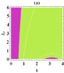
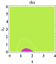
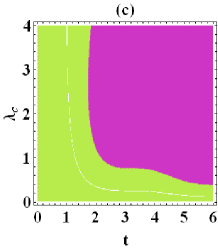
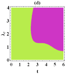
Figure 6: Left to right: $\mathcal{B}$ (a) for the atom-atom, (b) cavity-cavity, (c) reservoir-reservoir and (d) inter-system atom-cavity two-qubit partitions as a function of time $t$ and $\lambda_{c}$. $a$=$b$=$\frac{1}{\sqrt{2}}$. (a-c) and $a$=$\frac{1}{\sqrt{5}}$ for (d). The remaining intra-system atom-cavity, atom-reservoir and atom-cavity partitions did display any violation of the CHSH-Bell inequality (using Eq.(36). Regions (shaded purple) for which $\mathcal{B}$ exceeds 2 are Bell nonlocal. The white lines divides the fine interplay between the two competitive terms which appear in the Bell function of Eq.(36)

.

V.1 Classical and non-classical correlations

In this section, we evaluate the correlation measure known as the quantum discord, $\mathcal{D}$ for the two-qubit state in Eq.(23) and its cavity-cavity and reservoir-reservoir counterpart matrices. It is well known that the quantum discord is more robust as it captures nonlocal correlations not present in the entanglement measure zu ; ve1 ; ve2 , consequently it is non vanishing in states which has zero entanglement. The evaluation of $\mathcal{D}$ involves lengthy optimization procedures and analytical expressions are known exist only in a few limiting cases qali ; qali2 ; wangli .

The quantum mutual information of a composite state $\rho$ of two subsystems $A$ and $B$ is given by zu ; ve1 ; ve2 $\mathcal{I}(\rho)=S(\rho_{A})+S(\rho_{B})-S(\rho)$ for a density operator in $\mathcal{H}_{A}\otimes\mathcal{H}_{B}$. $\rho_{A}$ ($\rho_{B}$) is the reduced density matrix associated with $A$ ($B$) and $S(\rho_{i})$ (i=A,B) denotes the well known von Neumann entropy of the density operator $\rho_{i}$, where $S(\rho)=-{\rm tr}(\rho\log\rho)$. The mutual information can be written as

$$\mathcal{I}(\rho)=S(\rho_{B})-S(\rho|\rho_{A})$$ (37)

where $S(\rho|\rho_{A})=S(\rho)-S(\rho_{A})$ is the quantum conditional entropy.

After a series of measurements on $A$, the post measurement conditional state in $B$ is given by $\rho_{B|k}=\frac{1}{p_{k}}(\Pi_{k}\otimes\mathbb{I}_{B})\rho(\Pi_{k}\otimes\mathbb{I}_{B})$ where the probability $p_{k}={\rm tr}[\rho(\Pi_{k}\otimes\mathbb{I}_{B})]$ and $\{\Pi_{k}\}$ denote the one-dimensional projector indexed by the outcome $k$. A conditional entropy of the of the conditional state of subsystem $B$, $\rho_{B|k}$, is derived based on the cumulative effect of the mutually exclusive measurements on $A$ as $S(\rho|\{\Pi_{k}\})=\sum_{k}p_{k}S(\rho_{B|k})$. The measurement induced mutual information is therefore given by

$$\mathcal{I}(\rho|\{\Pi_{k}\})=S(\rho_{B})-S(\rho|\{\Pi_{k}\})$$ (38)

Eqs.(37) and (38) appear with slight differences due to incorporation of measurements in the definition for the latter.

The classical correlation measure based on optimal measurements is evaluated using $\mathcal{C}_{A}(\rho)=\sup_{\{\Pi_{k}\}}\mathcal{I}(\rho|\{\Pi_{k}\})$, and is the maximum information about one subsystem that can be obtained via measurements performed on the adjacent subsystem. The quantum discord which measures the non-classical correlations is given by the difference in $\mathcal{I}(\rho)$ and $\mathcal{C}_{A}(\rho)$

$$\mathcal{D}_{A}(\rho)=\mathcal{I}(\rho)-\mathcal{C}_{A}(\rho)$$ (39)

Following the analytical approach in earlier works qali ; qali2 ; wangli , expressions for the $C$ and $Q$ associated with the atom-atom bipartite system in Eq.(23) is obtained as

$$\mathcal{C}({\rho}_{a_{1},a_{2}}) = {H}(|a|^{2}(1-p))$$ (40)

$$- {H}\left(\frac{1}{2}\left[1+\sqrt{1-4|a|^{2}(1-p)p}\right]\right),$$

$$\mathcal{D}(\rho_{a_{1},a_{2}}) = {H}(|b|^{2}(1-p))-H(1-p)$$ (41)

$$- {H}\left(\frac{1}{2}\left[1+\sqrt{1-4|a|^{2}(1-p)p}\right]\right)$$

where the function $H(x)=-x\log_{2}x-(1-x)\log_{2}(1-x)$. Analogous expressions for $\mathcal{C}({\rho}_{c_{1},c_{2}}),\mathcal{D}({\rho}_{c_{1},c_{2}})$ and $\mathcal{C}({\rho}_{r_{1},r_{2}}),\mathcal{D}({\rho}_{r_{1},r_{2}})$ associated respectively with the cavity-cavity and reservoir-reservoir density matrices at time $t$, are obtained by respective substitutions $(1-p)\rightarrow q$ and $(1-p)\rightarrow\gamma_{d}$ in Eq. (40) and (41). At $t=$0 and $a=\frac{1}{\sqrt{2}}$, $\mathcal{C}({\rho}_{a_{1},a_{2}})$=$\mathcal{C}({\rho}_{a_{1},a_{2}})$=1 while the correlations of the cavity-cavity and reservoir-reservoir partitions are zero. Figures for the classical and quantum correlations as function of time $t$ for the analytical solutions ($p,q$) in Eqs.(15), (16) are shown below.

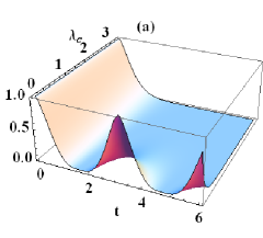
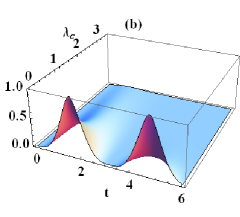
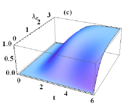
Figure 7: Classical correlation $\mathcal{C}({\rho})$ for the (a) atom-atom, (b) cavity-cavity, (c) reservoir-reservoir two-qubit partitions as a function of time $t$ and $\lambda_{c}$. $a$=$b$=$\frac{1}{\sqrt{2}}$.

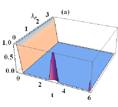
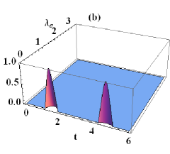
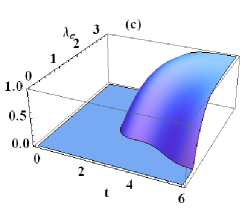
Figure 8: Quantum correlation $\mathcal{D}({\rho})$ for the (a) atom-atom, (b) cavity-cavity, (c) reservoir-reservoir two-qubit partitions as a function of time $t$ and $\lambda_{c}$. $a$=$b$=$\frac{1}{\sqrt{2}}$. There is transfer of the quantum discord from the atom-atom subsystem to the reservoir-reservoir partition.

Figures 7 and  8 show the expected shift in classical $\mathcal{C}({\rho})$ and quantum correlations $\mathcal{D}({\rho})$ away from the entangled atom-atom partition to the reservoir-reservoir partition. There exist larger regions (as function of time $t$ and $\lambda_{c}$) with zero quantum correlations than classical correlations. The appearance of $\mathcal{D}({\rho})$ is most significant in the reservoir-reservoir two-qubit partition as the system nears the exceptional point $\lambda_{c}\rightarrow$ 4. Comparison of Figure 6 a,b,c and Figures 7 and  8, show that for the considered subsystem partitions (atom-atom, cavity-cavity, reservoir-reservoir), Bell nonlocal regions can be matched with appearance of non-trivial classical and non-classical correlations. This is most noticeable in the reservoir-reservoir subsystem, and once again we reiterate that these results appear valid for the two-qubit partitioned subsystems.

V.2 Phase space approach of quantum dissipation

The current study has highlighted some salient features linking entities based on the abstract Hilbert space , and within the confines of the two-qubit partitions examined in this work. However, the validity of the results of dynamics in various subsystems is expected to be dependent on the form of the quantum master equation utilized in Eq. (8). Possible artifacts which arise from such Markovian forms have been examined by Kohen $et$ $al$. kohen , who analysed time evolving density operators transformed using several approaches including Redfield theories, the master equations of Agarwal agarwal and the semigroup theory of Lindblad lind , into Wigner phase space distribution functions. The Agarwal-Redfield (AR) equations of motion were seen to violate the semigroup form of Lindblad, showing that for certain initial states, the Redfield theory can violate simple positivity making it difficult to assign distinctly physical status for such states.

The Agarwal bath agarwal which is translational invariant and able to reach the thermal equilibrium limit, yields density matrix positivity for many initial conditions. However this bath system presents pathological effects as was noted in the density matrix negativity for a range of initial conditions at low temperatures talkner in a model system of one primary oscillator. These observations suggest possible association between the density matrix positivity and conditions which lead to the thermal equilibrium in system-bath correlations. In this regard, there is need to examine these links with incorporation of detailed attributes of the dissipative sink inherent in the the qubit-cavity-reservoir system of Eq. (1), in future investigations.

Finally, it is not entirely clear as to the role played by the bipartite partitioning of the six-qubit multipartite system (Eq. (21)) in the observed matching or non-matching of regions with noticeable non-locality, non-Markovianity and quantum correlations in the subsystems examined in this study. Future investigations should be aimed at higher dimensional density matrices (e.g. tripartite systems) and among all possible combinations of partitions, to see if the trends observed in two-qubit systems are indeed universal. This can be a formidable task, which may require a rigorous approach anand ; eis involving the mathematical formulations of the underlying abstract Hilbert space, to help form a basis for understanding the links between the quantum entities such as non-locality and non-Markovianity.

VI Application to Light-harvesting systems

The results of this study has immediate relevance to photosynthetic energy transfer in light-harvesting systems such as the Fenna-Matthews-Olson complex with moderate exciton-phonon coupling, and operation under physiological conditions. There is obvious similarity between the qubit-cavity-reservoir system in Eq. (1) and a photosynthetic model that constitutes the donor and acceptor protein pigment complexes with finite energy difference and a third party with a continuous frequency spectrum acting as the phonon-dissipative sink, and into which energy from the acceptor dissipates with time. The inclusion of comprehensive details incorporating the solvent relaxation rate as well as kinetic behaviors of the electron transfer mechanisms and dynamic bath effects in Eqs. (11) and  (11) will extend the applicability of the model in Eq. (8) to the more realistic environment of photosynthetic systems.

Earlier studies carupra ; caru1 have shown that attributes such as the non- Markovian interactions and quantum correlations contribute via a delicate interplay of quantum mechanical attributes and the environmental noise in bringing about an optimal performance. of the light harvesting complex. Non-Markovian effects were seen to reduce the transport efficiency while increasing the lifetime of entanglement carupra by disrupting the optimal balance of quantum and incoherent dynamics required for efficient energy transfer. In another study involving light harvesting systems reben2 , non-Markovian processes were noted to be most pronounced in the reorganization energy regime where the transfer efficiency is the highest, and linked with the preservation of coherence along critical pathways reben .

Results based on the exciton entanglement dynamics of the Fenna-Matthews-Olson (FMO) pigment-protein complex thilchem2 , indicate increased oscillations of entanglement in the non-Markovian regime, with implications for a link between non-Markovianity and large coherence times. Interestingly, an earlier work on optimizing energy transfer efficiency by Silbey and coworkers silbey , showed that the interplay of coherent dynamics and environmental noise resulted in the optimal energy transfer efficiency at an intermediate level for several variables in light-harvesting systems. In particular, the reorganization energy and the bath relaxation rate played critical roles in displaying a non-monotonic-dependence on energy transfer. Spatial correlation effects were noted silbey to optimize the energy transfer only during strong dissipation, highlighting differences in the roles played by spatial correlation and temporal correlations. In this regard, there is need to further examine the subtle links between non-Markovian dynamics and the effective system-bath coupling range, taking into consideration the site energy based electronic coupling correlations recom . Future investigations along these lines can employ the model developed through Eq. (8), (11) and  (11) as currently, the information on the exact mechanism by which non-Markovian processes act to bring about fast energy transport still remains unclear in light-harvesting systems.

The inclusion of quantum effects involving non-locality and non-classical correlations will provide greater insight to the recently proposed optical cavity quantum electrodynamics setup caruexpt to investigate energy transfer mechanism in biomolecules. There is also scope to examine similar quantum effects in a viable Grover-like search process grover via the exciton trapping mechanism at dissipative sink sites in photosynthetic systems. The incorporation of an approach incorporating non-Markovianity and the violation of the CHSH-Bell inequality may assist in developing new perspectives in interpreting experimental results obtained via two-dimensional electronic spectroscopy caram , 4-wave mixing measurements segale and the hybrid optical detector tomo which implements quantum detector tomography and characterizes simultaneous wave and photon-number sensitivities. To this end, future experimental work should incorporate the joint extraction of non-Markovian and Bell non-local features in biochemical systems, pending further refinement in optical techniques.

VII Discussion and Conclusion

In summary, we have studied the links between non-locality, non-Markovianity and quantum correlations of two initially correlated atomic qubits, each located in a single-mode leaky cavity and interacting with its own bosonic reservoir. The appearance of non-Markovianity is associated with a negative value for the the fidelity or trace-distance differences, and act only as qualitative signatures of deviation from a complete positve Markovian behavior. Results of the differences in non-Markovianity based on the two measures: fidelity and trace-distance shows its dependence on the distance metric, and regions of contractive quantum evolution vary according to the defined measure used to detect violations of Markovian dynamics.

The non-Markovian features in different two-qubit partitions (cavity-cavity and atom-reservoir partitions of the same subsystem, cavity-reservoir partition across different subsystem) show varying levels of erasure or enhancement of non-Markovianity depending on the cavity decay rate, $\lambda_{c}$. In particular, the exceptional point at which two eigenvalues merge, appear to signal the enhancement of non-Markovianity in selected regions (of time $t$ and $\lambda_{c}$) for the cavity-cavity partition. The changes in the vicinity of the exceptional point, also noted in quantum measurements thilaIOP , is significant as it may assist in distinguishing between processes with a classical origin and those with an intrinsically quantum mechanical coherence origin miller .

Results of the CHSH-Bell inequality computed for various two-qubit partitions show that enhanced non-locality present in a specific subsystem (e.g reservoir-reservoir matrix) appears in conjunction with non-Markovian evolution in an adjacent subsystem (e.g atom-reservoir matrix). The mismatch between non-locality and non-Markovianity for a given partition is in contrast to the matching between non-locality and quantum correlations for regions spanned by time $t$ and the cavity decay rate, $\lambda_{c}$. These results appear to provide weak signatures of subtle links between non-Markovianity, non-locality and non-classical correlations, bearing in mind that attempts to establish such links are very much reliant on the rigid formulation of the hidden variable model via the CHSH-Bell inequality relations in Eq. (36). Moreover the criteria used in this study provides only sufficient and not necessary tests of non-Markovianity, and also very much dependent on the initial state of correlations of the various subsystems. Currently, it is still not clear as to the origins of non-Markovianity as there is uncertainty as to whether information back-flow occurs due to the initial system-environment correlations or the intrinsic presence of specific dynamical features from which non-Markovianity emerge. Moreover, investigations involving tripartite states and higher dimensional states is needed to seek a definite conclusion on the perceived correlation/anti-correlation between non-locality, non-Markovianity and quantum discord. Lastly, the results obtained in this work highlight the need to adopt a unified model that incorporates non-Markovianity, non-locality and non-classical correlations, as an effective approach in examining high efficiencies of energy transfer observed in light-harvesting systems.

References

- (1) M. A. Nielsen and I. L. Chuang, Quantum computation and quantum information (Cambridge Univ. Press, Cambridge, 2002).
- (2) J. S. Bell, Physics 1, 195 (1964)
- (3) J. F. Clauser, M. A. Horne, A. Shimony, and R. A. Holt, Phys. Rev. Lett. 23, 880 (1969).
- (4) M. S. Williamson, L. Heaney, W. Son, Phys. Rev. A. 82, 032105 (2010).
- (5) F. Buscemi, Phys. Rev. Lett. 108, 200401 (2012)
- (6) E.C.G. Sudarshan, P.M. Mathews, J. Rau, Phys. Rev. 121, 920 (1961).
- (7) H.-P. Breuer and F. Petruccione The Theory of Open Quantum Systems (Oxford University Press, Oxford, 2001).
- (8) M. Choi, Positive Linear Maps on C*-Algebras, Can. J. Math Vol.24 No.3, 520-529 (1972)
- (9) G. Lindblad, Commun. Math. Phys. 48, 119 (1976).
- (10) K. Kraus, States, Effects, and Operations: Fundamental Notions of Quantum Theory, Springer (1983).
- (11) R. Alicki and K. Lendi, Quantum Dynamical Semigroups and Applications, Lecture Notes in Physics, Vol. 717 (2007).
- (12) T.F. Jordan, A. Shaji, E.C.G. Sudarshan, Phys. Rev. A 70, 1 (2004).
- (13) T. S. Cubitt, J. Eisert and M. M. Wolf, Communications in Math. Physics, 310, 383 (2012).
- (14) A. R. Usha Devi, A. K. Rajagopal, Sudha, Phys. Rev. A 83, 022109 (2011).
- (15) J. Li, G. McKeown, F. L. Semiao and M. Paternostro, Phys. Rev. A 85, 022116 (2012).
- (16) L. Mazzola, B. Bellomo, R. Lo Franco, and G. Compagno, Phys. Rev. A 81, 052116 (2010).
- (17) F. Caruso, A. W. Chin, A. Datta, S. F. Huelga, and M. B. Plenio, Phys. Rev. A 81, 062346 (2010).
- (18) P. Rebentrost, A. Aspuru-Guzik, J. Chem. Phys.134, 101103 (2011).
- (19) H. P. Breuer, E. M. Laine, and J. Piilo, Phys. Rev. Lett.103, 210401 (2009).
- (20) M.M. Wolf, J. Eisert, T.S. Cubitt, J.I. Cirac, Phys. Rev. Lett. 101, 150402 (2008).
- (21) A. Rivas, S. F. Hulega and M. B. Plenio, Phys. Rev. Lett. 105, 050403 (2010).
- (22) Hao-Sheng Zeng, Ning Tang, Yan-Ping Zheng, and Guo-You Wang Phys. Rev. A 84, 032118 (2011).
- (23) D. Chruscinski, A. Kossakowski and A. Rivas, Phys. Rev. A 83, 052128 (2011).
- (24) X. M. Lu, X. G. Wang, and C. P. Sun, Phys. Rev. A 82, 042103 (2010).
- (25) A. Thilagam, J. Chem. Phys. 136, 175104 (2012).
- (26) R. Lo Franco, B. Bellomo, E. Andersson, and G. Compagno, Phys. Rev. A 85, 032318 (2012).
- (27) H. Ollivier and W. H. Zurek, Phys. Rev. Lett. 88, 017901 (2001).
- (28) A. K. Rajagopal, A. R. U. Devi, R. W. Rendell, Phys. Rev. A 82, 042107 (2010).
- (29) R. Jozsa, J. Mod. Optics, 41, 2315 (1994).
- (30) W. D. Heiss and A L Sannino, J. Phys. A: Math. Gen. 23 1167 (1990).
- (31) H. Feshbach, Ann. Phys. 5, 357 (1958).
- (32) M. Scala, B. Militello, A. Messina, J. Piilo, and S. Maniscalco, Phys. Rev. A.75, 013811 (2007).
- (33) H.J. Carmichael, Statistical Methods in Quantum Optics 2, (Springer, Berlin, 2008).
- (34) H. J. Carmichael, Phys. Rev. Lett. 70, 2273 (1993).
- (35) J. Dalibard, Y. Castin, and K. Molmer, Phys. Rev. Lett. 68, 580 (1992).
- (36) C. Di Fidio, W. Vogel, M. Khanbekyan and D. G. Welsch. Phys. Rev. A 77, 043822 (2008).
- (37) A. Thilagam, J. Chem. Phys. 136, 065104 (2012).
- (38) V. Vedral and M. Plenio, Phys. Rev. A 57, 1619 (1998).
- (39) B. Bellomo, R. Lo Franco, and G. Compagno, Phys. Rev. A 78, 062309 (2008); Phys. Lett. A 374, 3007 (2010).
- (40) L. Henderson and V. Vedral, J. Phys. A 34, 6899 (2001).
- (41) V. Vedral, Phys. Rev. Lett. 90, 050401 (2003).
- (42) M. Ali, A. R. P. Rau, and G. Alber, Phys. Rev. A 81, 042105 (2010).
- (43) M. Ali, A. R. P. Rau, and G. Alber, Phys. Rev. A 82, 069902(E) (2010).
- (44) C. Z. Wang, C. X. Li, L. Y. Nie and J. F. Li, J. Phys. B: At. Mol. Opt. Phys. 44, 015503 (2011).
- (45) D. Kohen, Marston, and D. J. Tannor, J. Chem. Phys. 107, 5236 (1997).
- (46) G. S. Agarwal, Phys. Rev. A 2, 2038 (1970); Phys. Rev. A 4, 739 (1971); Phys. Rev. 178, 2025 (1969).
- (47) P. Talkner, Ann. Phys. N.Y.! 169, 390 1986!.
- (48) J. Anandan and Y. Aharonov, Phys. Rev. Lett. 65, 1697 (1990).
- (49) F. Caruso, A. W. Chin, A. Datta, S. F. Huelga, and M. B. Plenio, J. Chem. Phys. 131, 105106 (2009).
- (50) P. Rebentrost, M. Mohseni, and A. Aspuru-Guzik, J. Phys. Chem. B 113, 9942 (2009).
- (51) J. Wu, F. Liu, Y. Shen, J. Cao and R. J. Silbey, New J. Phys.12,105012 (2010)
- (52) X. Chen and R. J. Silbey, J.Chem.Phys 132, 204503 (2010)
- (53) F. Caruso, S. K. Saikin, E. Solano, S. F. Huelga, A. Aspuru-Guzik, and M. B. Plenio Phys. Rev. B 85, 125424 (2012)
- (54) A. Thilagam, Phys. Rev. A 81, 032309 (2010).
- (55) J. R. Caram, A. F. Fidler, and G. S. EngeL, J. Chem. Phys. 137, 024507 (2012).
- (56) D. Segale and V. A. Apkarian, J. Chem. Phys. 135, 024203 (2011).
- (57) L. Zhang, H. B. Coldenstrodt-Ronge, A. Datta, G. Puentes, J. S. Lundeen, X.-Min Jin, B. J. Smith, M. B. Plenio and I. A. Walmsley Nature Photonics 6, 364 (2012)
- (58) A. Thilagam, J. Phys. A: Math. Theor. 45 444031 (2012).
- (59) W. H. Miller, J. Chem. Phys. 136, 210901 (2012).