A numerical framework for diffusion-controlled bimolecular-reactive systems to enforce maximum principles and the non-negative constraint

Abstract.

We present a novel computational framework for diffusive-reactive systems that satisfies the non-negative constraint and maximum principles on general computational grids. The governing equations for the concentration of reactants and product are written in terms of tensorial diffusion-reaction equations. We restrict our studies to fast irreversible bimolecular reactions. If one assumes that the reaction is diffusion-limited and all chemical species have the same diffusion coefficient, one can employ a linear transformation to rewrite the governing equations in terms of invariants, which are unaffected by the reaction. This results in two uncoupled tensorial diffusion equations in terms of these invariants, which are solved using a novel non-negative solver for tensorial diffusion-type equations. The concentrations of the reactants and the product are then calculated from invariants using algebraic manipulations. The novel aspect of the proposed computational framework is that it will always produce physically meaningful non-negative values for the concentrations of all chemical species. Several representative numerical examples are presented to illustrate the robustness, convergence, and the numerical performance of the proposed computational framework. We will also compare the proposed framework with other popular formulations. In particular, we will show that the Galerkin formulation (which is the standard single-field formulation) does not produce reliable solutions, and the reason can be attributed to the fact that the single-field formulation does not guarantee non-negative solutions. We will also show that the clipping procedure (which produces non-negative solutions but is considered as a variational crime) does not give accurate results when compared with the proposed computational framework.

1. INTRODUCTION AND MOTIVATION

Mixing of chemical species across plume boundaries has a major influence on the fate of reactive pollutants in subsurface flows. In many practical cases, the intrinsic rate of reaction is fast compared with other relevant time scales and hence the reaction may be assumed instantaneous (e.g., see references [1, 2]). Mixing is commonly modeled as an anisotropic Fickian diffusion process, with the effective diffusion coefficient aligned with the flow velocity (termed the longitudinal hydrodynamic dispersion coefficient) being much larger than the transverse components. Moreover, the small-scale spatial variability of permeability in real aquifers leads to highly heterogeneous velocity fields, which means that the principal directions of the diffusion tensor will vary in space and will not be aligned with the numerical grid. It has also been demonstrated that accurate treatment of dispersive mixing is crucial for computing the large-time spatial extent of the contaminant plume, which is a very important measure of the contaminant risk and thus of great interest to government regulators and the general public (e.g., see Reference [3]). It is well-known that heterogeneity and anisotropy lead to irregular plume boundaries, which enhance mixing-controlled reactions through increasing the interfacial area of the plume. It is, therefore, crucial to capture heterogeneity and anisotropy in order to properly model reactive transport in hydrogeological systems.

One can capture heterogeneity computationally through adequate mesh refinement or by employing multiscale methods (for example, see references [4, 5, 6, 7]). Although simulating flow and transport in highly heterogeneous porous media is still an active area of research, we shall not address this aspect in this paper. We shall employ meshes that are fine enough to be able to resolve heterogeneity. This paper focuses on resolving anisotropy to be able to accurately predict the fate of chemical species. We shall model the spatial and temporal variation of chemical species through diffusion-reaction equations.

Diffusive-reactive equations arise naturally in modeling biological [8, 9], chemical [10, 11], and physical [12] systems. The areas of application of diffusion-reaction systems range from contaminant transport [13], semiconductors [14], combustion theory [15] to biological population dynamics [16]. It is well-known that these types of equations can exhibit complex and well-ordered structures/patterns [17, 12]. A lot of effort has also been put into the mathematical analysis of diffusive-reactive systems. Many qualitative mathematical properties (e.g., comparison principles, maximum principles, the non-negative constraint) have been obtained for these systems [18, 19, 20]. A detailed discussion on mathematical aspects of diffusive-reactive systems is beyond the scope of this paper and is not central to the present study.

1.1. Fast bimolecular reactions

The main aim of this paper is to present a robust computation framework to obtain physically meaningful numerical solutions for diffusive-reactive systems. We shall restrict to bimolecular fast reactions for which the rate of reaction is controlled by diffusion of the two chemical species. Fast irreversible bimolecular diffusion-reaction equations come under the class of diffusion-controlled reactions [21, 22]. Examples of such systems include ionic reactions occurring in aqueous solutions such as acid-base reactions [23, 24], polymer chain growth kinetics [25], catalytic reactions [26] and enzymatic reactions [27]. In such systems the formation of the product is much faster than the diffusion of the reactants. In this paper we are only concerned about homogeneous reactions (i.e., the reactants are all in the same phase). Modeling diffusive-reactive systems in which reactions are heterogeneous (i.e., the reactants are in different phases) by incorporating the surface effects of the reactants (for example, see references [28, 29, 30, 31, 32, 33, 34]) is beyond the scope of the present paper but will be considered in our future works.

Some main challenges in solving a system of diffusion-reaction equations are as follows:

1. Anisotropy: Developing robust computational frameworks for highly anisotropic diffusive-reactive systems is certainly gaining prominence. However, caution needs to be exercised in selecting numerical formulations to avoid negative values for the concentration of the chemical species. Many popular numerical schemes such as the standard single-field formulation [35], the lowest order Raviart-Thomas formulation [36], and the variational multiscale mixed formulation [37, 38] give unphysical negative values for the concentration even for pure diffusion equations [39]. Furthermore, mesh refinement (either $h$-refinement [40] or $p$-refinement [41]) will not overcome the problem of negative values for the concentration. Keeping in mind about these concerns and developing a robust framework for diffusive-reactive systems is a challenging task.

2. Nonlinearity: The equations governing for these systems are coupled and nonlinear (see equations (2.2a)–(2.2d), which are presented in a subsequent section). The solutions to these diffusive-reactive systems can exhibit steep gradients [42], and a robust numerical solution procedure should be able to handle such features.

3. Scale dependence: These types of systems can exhibit multiple spatial and temporal scales. For example, the diffusion process can be much slower than the chemical reactions. Therefore, the numerical techniques should be able to resolve these multiple scales. Compared to fast reactions, different solution strategies are required for moderate and slow reactions, which are typically easier to solve due to smaller gradients. Construction of adaptive numerical techniques that take the advantage of specific reaction kinetics and simultaneously satisfying the underlying mathematical properties is still in its infancy.

4. Bifurcations, physical instabilities and pattern formations: These systems are capable of exhibiting physical instabilities, and even chaos [18].

We shall overcome the first challenge by employing a novel non-negative solver that ensures physically meaningful non-negative values for the concentration of chemical species. We employ a transformation of variables, which will overcome the second and third challenges. We solve problems that do not exhibit physical instabilities and chaos. Although considerable progress has been made in developing numerical solutions of diffusive-reactive systems [43, 44], none of these studies addressed the difficulties in obtaining non-negative solutions especially under strong anisotropy, which is the main focus of this paper. The following systematic approach has been employed to achieve the desired goal. The reactions are assumed to be fast and bimolecular. The concentration of reactants and product are governed by tensorial diffusion-reaction equations, and by an appropriate stoichiometric relationship. The three coupled tensorial diffusion-reaction equations are rewritten in terms of invariants, which are unaffected by the reaction. This procedure results in two uncoupled tensorial diffusion equations in terms of the invariants. A robust non-negative solver is employed to solve these two uncoupled tensorial diffusion equations following the ideas outlined in references [39, 40]. The concentrations of the reactants and product are then calculated using simple algebraic relations given by the transformation that is employed.

1.2. An outline of the paper

The remainder of the paper is organized as follows. In Section 2, we first present the governing equations for a diffusive-reactive system in a general setting. We later restrict the study to fast bimolecular reactions, and deduce the corresponding governing equations. In Section 3, we present a novel non-negative computational framework for solving diffusive-reactive systems. Section 4 provides a theoretical discussion on the optimization-based solver for enforcing maximum principles. Representative numerical results are presented in Section 5, and conclusions are drawn in Section 6.

The standard symbolic notation is adopted in this paper. We shall denote scalars by lowercase English alphabet or lowercase Greek alphabet (e.g., concentration $c$ and density $\rho$). We shall make a distinction between vectors in the continuum and finite element settings. Similarly, a distinction is made between second-order tensors in the continuum setting versus matrices in the context of the finite element method. The continuum vectors are denoted by lower case boldface normal letters, and the second-order tensors will be denoted using upper case boldface normal letters (e.g., vector $\mathbf{x}$ and second-order tensor $\mathbf{D}$). In the finite element context, we shall denote the vectors using lower case boldface italic letters, and the matrices are denoted using upper case boldface italic letters (e.g., vector $\boldsymbol{v}$ and matrix $\boldsymbol{K}$). It should be noted that repeated indices do not imply summation. (That is, Einstein’s summation convention is not employed in this paper.) Other notational conventions adopted in this paper are introduced as needed.

2. GOVERNING EQUATIONS: DIFFUSIVE-REACTIVE SYSTEMS

We now present governing equations of a simple diffusive-reactive system in a rigid porous medium. Let $\Omega\subset\mathbb{R}^{nd}$ be an open bounded domain, where “$nd$” denotes the number of spatial dimensions. The boundary is denoted by $\partial\Omega$, which is assumed to be piecewise smooth. Mathematically, $\partial\Omega:=\bar{\Omega}-\Omega$, where $\bar{\Omega}$ is the set closure of $\Omega$. A spatial point in $\bar{\Omega}$ is denoted by $\mathbf{x}$. The divergence and gradient operators with respect to $\mathbf{x}$ are, respectively, denoted by $\mathrm{div}[\cdot]$ and $\mathrm{grad}[\cdot]$. The unit outward normal to the boundary is denoted by $\mathbf{n}(\mathbf{x})$. Let $t\in\,]0,\mathcal{I}[$ denote the time, where $\mathcal{I}$ is the length of time of interest. We shall write the governing equations for the individual chemical species and for the mixture on the whole using the mathematical framework provided by the theory of interacting continua [45].

We shall assume that there are $n$ chemical species, which include both reactants and product(s). We shall denote the molar mass of the $i$-th species by $\zeta_{i}$. The mass concentration of the $i$-th species at the spatial position $\mathbf{x}$ and time $t$ is denoted by $\varphi_{i}(\mathbf{x},t)$. The molar concentration of the $i$-th species is denoted by $c_{i}(\mathbf{x},t)$ and is defined as follows:

$$c_{i}(\mathbf{x},t):=\frac{\varphi_{i}(\mathbf{x},t)}{\zeta_{i}}$$ (2.1)

For each chemical species $(i=1,\cdots,n)$, the boundary is divided into two complementary parts: $\Gamma^{\mathrm{D}}_{i}$ and $\Gamma^{\mathrm{N}}_{i}$. $\Gamma^{\mathrm{D}}_{i}$ is that part of the boundary on which concentration for the $i$-th species is prescribed, and $\Gamma^{\mathrm{N}}_{i}$ is the part of the boundary on which the flux for the $i$-th chemical species is prescribed. For well-posedness and uniqueness of the solution, we require $\Gamma^{\mathrm{D}}_{i}\cap\Gamma^{\mathrm{N}}_{i}=\emptyset$, $\Gamma^{\mathrm{D}}_{i}\cup\Gamma^{\mathrm{N}}_{i}=\partial\Omega$, and $\mathrm{meas}(\Gamma^{\mathrm{D}}_{i})>0$. The governing equations for the fate of the $i$-th chemical species can be written as follows:

$$\frac{\partial\varphi_{i}}{\partial t}-\mathrm{div}[\mathbf{D}(\mathbf{x})\,\mathrm{grad}[\varphi_{i}]]=m_{i}(\mathbf{x},t)+g_{i}(\mathbf{x},\varphi_{1},\cdots,\varphi_{n},t)\quad\mathrm{in}\;\Omega\times]0,\mathcal{I}[$$ (2.2a)

$$\varphi_{i}(\mathbf{x},t)=\varphi^{\mathrm{p}}_{i}(\mathbf{x},t)\quad\mathrm{on}\;\Gamma^{\mathrm{D}}_{i}\times]0,\mathcal{I}[$$ (2.2b)

$$\mathbf{n}(\mathbf{x})\cdot\mathbf{D}(\mathbf{x})\,\mathrm{grad}[\varphi_{i}]=\vartheta^{\mathrm{p}}_{i}(\mathbf{x},t)\quad\mathrm{on}\;\Gamma^{\mathrm{N}}_{i}\times]0,\mathcal{I}[$$ (2.2c)

$$\varphi_{i}(\mathbf{x},t=0)=\varphi^{0}_{i}(\mathbf{x})\quad\mathrm{in}\;\Omega$$ (2.2d)

where $\mathbf{D}(\mathbf{x})$ is the diffusivity tensor, $\varphi^{\mathrm{p}}_{i}(\mathbf{x},t)$ is the prescribed mass concentration on the boundary, $\vartheta^{\mathrm{p}}_{i}(\mathbf{x},t)$ is the prescribed mass concentration flux on the boundary, $\varphi^{0}_{i}(\mathbf{x})$ is the (prescribed) initial condition, $g_{i}(\mathbf{x},\varphi_{1},\cdots,\varphi_{n},t)$ is the rate of production/depletion of the $i$-th species due to chemical reactions, and $m_{i}(\mathbf{x},t)$ is the prescribed external volumetric mass supply for the $i$-th species. Equations (2.2a)–(2.2d) are, respectively, the balance of mass, the Dirichlet boundary condition, the Neumann boundary condition, and the initial condition for the $i$-th chemical species. The governing equation for the balance of mass for the mixture on the whole takes the following form:

$$\sum_{i=1}^{n}g_{i}(\mathbf{x},\varphi_{1},\cdots,\varphi_{n},t)=0\quad\forall\mathbf{x}\in\Omega,\;\forall t\in]0,\mathcal{I}[$$ (2.3)

In Engineering and Applied Sciences, the above system of equations (2.2a)–(2.2d) is commonly referred to as time-dependent or non-stationary diffusion-reaction equations. In the theory of partial differential equations, the above system of equations is referred to as coupled semilinear parabolic partial differential equations [18]. These types of equations are capable of exhibiting many interesting and complex features like instabilities, bifurcations, and even chaos (for example, see Pao [18]). However, in this paper we shall focus only on three interrelated mathematical properties that these types of equations satisfy: maximum principles, comparison principles, and the non-negative constraint.

For completeness, we shall document the assumptions in obtaining the governing equations (2.2a)–(2.2d) under the mathematical framework offered by the theory of interacting continua. The main assumptions are as follows:

1. The porous medium in which the reaction takes place is assumed to be rigid.

2. The flow aspects in the porous media are neglected. Hence, the advection velocity of each chemical species in the mixture is zero.

3. The chemical species do not take partial stresses.

4. The diffusion process is based on the Fickian model.

5. The diffusivity tensor $\mathbf{D}(\mathbf{x})$ is the same for all the chemical species, which is the case with many diffusive-reactive systems. (However, it should be noted that in some chemical and biological diffusive-reactive systems the diffusivity tensor $\mathbf{D}(\mathbf{x})$ will be different for different species.)

One can obtain a hierarchy of more complicated models by relaxing/generalizing one or more of the aforementioned assumptions, which will be considered in our future works. We shall now restrict our study to bimolecular reactions.

2.1. Bimolecular reactions

Bimolecular reactions are reactions involving two reactant molecules. To this end, consider two chemical species $A$ and $B$ that react irreversibly to give the product $C$ according to the following stoichiometric relationship:

$$n_{A}\,A\,+\,n_{B}\,B\rightarrow n_{C}\,C$$ (2.4)

where $n_{A}$, $n_{B}$ and $n_{C}$ are (positive) stoichiometric coefficients. The rate of the chemical reaction is denoted by $r$, which (in general) can be a nonlinear function of the concentrations of the chemical species involved in the reaction. For a bimolecular reaction, one can write the rate of the reaction at the spatial point $\mathbf{x}$ and time $t$ as follows:

$$r(\mathbf{x},c_{A}(\mathbf{x},t),c_{B}(\mathbf{x},t),c_{C}(\mathbf{x},t),t)=-\frac{g_{A}}{n_{A}\zeta_{A}}=-\frac{g_{B}}{n_{B}\zeta_{B}}=+\frac{g_{C}}{n_{C}\zeta_{C}}$$ (2.5)

For bimolecular reactions, the governing equations (2.2a)–(2.2d) can be rewritten as follows:

$$\frac{\partial c_{A}}{\partial t}-\mathrm{div}[\mathbf{D}(\mathbf{x})\,\mathrm{grad}[c_{A}]]=f_{A}(\mathbf{x},t)-n_{\small{A}}\,r\quad\mathrm{in}\;\Omega\times]0,\mathcal{I}[$$ (2.6a)

$$\frac{\partial c_{B}}{\partial t}-\mathrm{div}[\mathbf{D}(\mathbf{x})\,\mathrm{grad}[c_{B}]]=f_{B}(\mathbf{x},t)-n_{\small{B}}\,r\quad\mathrm{in}\;\Omega\times]0,\mathcal{I}[$$ (2.6b)

$$\frac{\partial c_{C}}{\partial t}-\mathrm{div}[\mathbf{D}(\mathbf{x})\,\mathrm{grad}[c_{C}]]=f_{C}(\mathbf{x},t)+n_{\small{C}}\,r\quad\mathrm{in}\;\Omega\times]0,\mathcal{I}[$$ (2.6c)

$$c_{i}(\mathbf{x},t)=c^{\mathrm{p}}_{i}(\mathbf{x},t)\quad\mathrm{on}\;\Gamma^{\mathrm{D}}_{i}\times]0,\mathcal{I}[\quad(i=A,\,B,\;C)$$ (2.6d)

$$\mathbf{n}(\mathbf{x})\cdot\mathbf{D}(\mathbf{x})\,\mathrm{grad}[c_{i}]=h^{\mathrm{p}}_{i}(\mathbf{x},t)\quad\mathrm{on}\;\Gamma^{\mathrm{N}}_{i}\times]0,\mathcal{I}[\quad(i=A,\,B,\;C)$$ (2.6e)

$$c_{i}(\mathbf{x},t=0)=c^{0}_{i}(\mathbf{x})\quad\mathrm{in}\;\Omega\quad(i=A,\,B,\;C)$$ (2.6f)

where the prescribed molar supply and the prescribed molar initial condition for the $i$-th species are, respectively, defined as follows:

$$f_{i}(\mathbf{x},t) =\frac{m_{i}(\mathbf{x},t)}{\zeta_{i}}$$ (2.7)

$$c_{i}^{0}(\mathbf{x}) =\frac{\varphi^{0}_{i}(\mathbf{x})}{\zeta_{i}}$$ (2.8)

and the prescribed molar concentration and the prescribed molar concentration flux for the $i$-th species on the boundary are, respectively, defined as follows:

$$c^{\mathrm{p}}_{i}(\mathbf{x},t) =\frac{\varphi^{\mathrm{p}}_{i}(\mathbf{x},t)}{\zeta_{i}}$$ (2.9)

$$h^{\mathrm{p}}_{i}(\mathbf{x},t) =\frac{\vartheta^{\mathrm{p}}_{i}(\mathbf{x},t)}{\zeta_{i}}$$ (2.10)

Before we present the proposed computational framework, few remarks are in order.

Remark 2.1.

A bimolecular equation, in its most general form, takes the following form:

$$n_{A}A+n_{B}B\rightarrow n_{C}C+n_{D}D+\cdots$$ (2.11)

We considered bimolecular reactions of the form given in equation (2.4) just to make the presentation simpler. However, it should be emphasized that with a simple and straightforward extension the framework can handle bimolecular reactions of the form given by equation (2.11).

Remark 2.2.

One can handle stoichiometry using a stoichiometric matrix (for example, see references [45, 46]). This approach will be convenient and appropriate for complicated chemical reactions that involve multiple stages, multiple chemical species, and intermediate complexes. Herein, we shall not take such an approach, as the reaction is relatively simpler.

Remark 2.3.

The mathematical model presented in this section, and the computational framework proposed in this paper can be used to obtain numerical solutions and perform predictive simulations for various practical problems proposed in the literature. To name a few: transverse mixing-limited chemical reactions in groundwater and aquifers [47, 48, 49], and mixing-controlled bioreactive transport in heterogeneous porous media for engineered bioremediation and contaminant degradation scenarios [3, 50, 51, 52, 53, 54] Other practically important examples include acid-base reactions [55], atmospheric chemical transport [56], chemistry of marine boundary layer [57], drinking water treatment [58], and reaction enhancement through chaotic flows [59, 60, 61].

3. PROPOSED COMPUTATIONAL FRAMEWORK

We now present a robust numerical framework to solve bimolecular diffusive-reactive systems given by equations (2.6a)–(2.6f) that will produce physically meaningful non-negative solutions for the concentration of chemical species on general computational grids. As mentioned earlier, we shall restrict our studies to fast reactions. By fast reactions we mean that the rate of the chemical reaction is much faster than the rate of the diffusion process.

3.1. A non-negative invariant set, and uncoupled equations

Using an appropriate linear transformation, one can obtain two independent invariants, which are unaffected by the chemical reaction. As we shall see later that these invariants will be governed by uncoupled linear diffusion equations. For the bimolecular diffusive-reactive system (2.6), one can construct three different sets of independent invariants. Herein, we shall employ the set of independent invariants that inherits the non-negative property, and the corresponding linear transformation can be written as follows:

$$c_{F} :=c_{A}+\left(\frac{n_{A}}{n_{C}}\right)c_{C}$$ (3.1a)

$$c_{G} :=c_{B}+\left(\frac{n_{B}}{n_{C}}\right)c_{C}$$ (3.1b)

Remark 3.1.

Let us denote the other two sets of independent invariants by $(U,V)$ and $(M,N)$, which can be devised as follows:

$$c_{U} :=c_{A}-\left(\frac{n_{A}}{n_{B}}\right)c_{B},\;c_{V}:=c_{A}+\left(\frac{n_{A}}{n_{C}}\right)c_{C}$$ (3.2a)

$$c_{M} :=c_{B}-\left(\frac{n_{B}}{n_{A}}\right)c_{A},\;c_{N}:=c_{B}+\left(\frac{n_{B}}{n_{C}}\right)c_{C}$$ (3.2b)

As one can see from the above expressions, $c_{U}$ and $c_{M}$ need not be always non-negative, which is not unphysical as $U$ and $M$ do not refer to any chemical species. They are just convenient mathematical quantities, and the possibility of negative values for these quantities is just a consequence of their mathematical definitions. We shall not use the above invariants as they do not possess the non-negative property, and hence are not appropriate to be used in a non-negative solver for diffusion-type equations.

In the remainder of this paper, we shall assume that $\Gamma^{\mathrm{D}}_{A}=\Gamma^{\mathrm{D}}_{B}=\Gamma^{\mathrm{D}}_{C}$, and shall denote them by $\Gamma^{\mathrm{D}}$ for notational convenience. Similarly, we shall assume that $\Gamma^{\mathrm{N}}_{A}=\Gamma^{\mathrm{N}}_{B}=\Gamma^{\mathrm{N}}_{C}$, and shall denote them by $\Gamma^{\mathrm{N}}$. These assumptions will facilitate application of the linear transformation to the prescribed boundary conditions $c^{\mathrm{p}}_{i}(\mathbf{x},t)$ and $h^{\mathrm{p}}_{i}(\mathbf{x},t)$ ($i=A,\,B,\,C$). Using straightforward manipulations on equations (2.6a)–(2.6f) based on the non-negative invariant set (3.1) and appealing to the above assumptions, one can show that the governing equations for the invariant $F$ can be written as follows:

$$\frac{\partial c_{F}}{\partial t}-\mathrm{div}[\mathbf{D}(\mathbf{x})\,\mathrm{grad}[c_{F}]]=f_{F}(\mathbf{x},t)\quad\mathrm{in}\;\Omega\times]0,\mathcal{I}[$$ (3.3a)

$$c_{F}(\mathbf{x},t)=c_{F}^{\mathrm{p}}(\mathbf{x},t):=c^{\mathrm{p}}_{A}(\mathbf{x},t)+\left(\frac{n_{A}}{n_{C}}\right)c^{\mathrm{p}}_{C}(\mathbf{x},t)\quad\mathrm{on}\;\Gamma^{\mathrm{D}}\times]0,\mathcal{I}[$$ (3.3b)

$$\mathbf{n}(\mathbf{x})\cdot\mathbf{D}(\mathbf{x})\,\mathrm{grad}[c_{F}]=h^{\mathrm{p}}_{F}(\mathbf{x},t):=h^{\mathrm{p}}_{A}(\mathbf{x},t)+\left(\frac{n_{A}}{n_{C}}\right)h^{\mathrm{p}}_{C}(\mathbf{x},t)\quad\mathrm{on}\;\Gamma^{\mathrm{N}}\times]0,\mathcal{I}[$$ (3.3c)

$$c_{F}(\mathbf{x},t=0)=c^{0}_{F}(\mathbf{x}):=c^{0}_{A}(\mathbf{x})+\left(\frac{n_{A}}{n_{C}}\right)c^{0}_{C}(\mathbf{x})\quad\mathrm{in}\;\Omega$$ (3.3d)

Similarly, the governing equations for the invariant $G$ take the following form:

$$\frac{\partial c_{G}}{\partial t}-\mathrm{div}[\mathbf{D}(\mathbf{x})\,\mathrm{grad}[c_{G}]]=f_{G}(\mathbf{x},t)\quad\mathrm{in}\;\Omega\times]0,\mathcal{I}[$$ (3.4a)

$$c_{G}(\mathbf{x},t)=c^{\mathrm{p}}_{G}(\mathbf{x},t):=c^{\mathrm{p}}_{B}(\mathbf{x},t)+\left(\frac{n_{B}}{n_{C}}\right)c^{\mathrm{p}}_{C}(\mathbf{x},t)\quad\mathrm{on}\;\Gamma^{\mathrm{D}}\times]0,\mathcal{I}[$$ (3.4b)

$$\mathbf{n}(\mathbf{x})\cdot\mathbf{D}(\mathbf{x})\,\mathrm{grad}[c_{G}]=h^{\mathrm{p}}_{G}(\mathbf{x},t):=h^{\mathrm{p}}_{B}(\mathbf{x},t)+\left(\frac{n_{B}}{n_{C}}\right)h^{\mathrm{p}}_{C}(\mathbf{x},t)\quad\mathrm{on}\;\Gamma^{\mathrm{N}}\times]0,\mathcal{I}[$$ (3.4c)

$$c_{G}(\mathbf{x},t=0)=c^{0}_{G}(\mathbf{x}):=c^{0}_{B}(\mathbf{x})+\left(\frac{n_{B}}{n_{C}}\right)c^{0}_{C}(\mathbf{x})\quad\mathrm{in}\;\Omega$$ (3.4d)

In the above equations, the prescribed molar supplies for the invariants $F$ and $G$ in terms of the chemical species $A$, $B$, and $C$ take the following form:

$$f_{F}(\mathbf{x},t)=f_{A}(\mathbf{x},t)+\left(\frac{n_{A}}{n_{C}}\right)f_{C}(\mathbf{x},t)$$ (3.5a)

$$f_{G}(\mathbf{x},t)=f_{B}(\mathbf{x},t)+\left(\frac{n_{B}}{n_{C}}\right)f_{C}(\mathbf{x},t)$$ (3.5b)

3.2. Specializing on fast bimolecular reactions

Recall that by a fast reaction we mean that the time scale of the reaction is much faster than the time scales associated with the diffusion process of the chemical species. Hence, for bimolecular reactions that are fast, it is a good approximation to assume that the species $A$ and $B$ cannot co-exist at any given instance of time at the same location $\mathbf{x}$. This assumption will be exact in the limit of infinitely fast / instantaneous reactions. Using equations (3.1a)–(3.1b), one can rewrite the whole problem for fast irreversible bimolecular fast reactions in terms of the conserved quantities $c_{F}(\mathbf{x},t)$ and $c_{G}(\mathbf{x},t)$ as follows:

$$c_{A}(\mathbf{x},t)=\mathrm{max}\left[c_{F}(\mathbf{x},t)-\left(\frac{n_{A}}{n_{B}}\right)c_{G}(\mathbf{x},t),\,0\right]$$ (3.6a)

$$c_{B}(\mathbf{x},t)=\left(\frac{n_{B}}{n_{A}}\right)\;\mathrm{max}\left[-c_{F}(\mathbf{x},t)+\left(\frac{n_{A}}{n_{B}}\right)c_{G}(\mathbf{x},t),\,0\right]$$ (3.6b)

$$c_{C}(\mathbf{x},t)=\left(\frac{n_{C}}{n_{A}}\right)\;\left(c_{F}(\mathbf{x},t)-c_{A}(\mathbf{x},t)\right)$$ (3.6c)

It should be noted that the original coupled diffusive-reactive system (2.6) is nonlinear and the solution procedure to obtain the concentrations of $A$, $B$, and $C$ is still nonlinear. This is because of the fact that $\mathrm{max}[\cdot,\cdot]$ is a nonlinear operator. However, the obvious advantage is that the resulting equations are much simpler to solve.

Before we discuss about the non-negative constraint, we shall introduce relevant notation. Let $D_{T}:=\Omega\times]0,\mathcal{I}]$, and $S_{T}:=\partial\Omega\times]0,\mathcal{I}]$. Let $C^{m}(K)$ denote the set of all $m$-times continuously differentiable functions on an open set $K$. The set of all continuous functions on the (set) closure of $K$ is denoted by $C(\bar{K})$. The set of all functions that are $m$-times continuously differentiable in $\mathbf{x}\in\Omega$ and $l$-times continuously differentiable in $t\in]0,\mathcal{I}]$ is denoted by $C^{m,l}(D_{T})$. From the theory of partial differential equations we have the following non-negative lemma for (pure) transient diffusion-type equations.

Lemma 3.2 (The non-negative constraint for transient diffusion equation).

Let $c(\mathbf{x},t)\in C^{2,1}(D_{T})\cap C(\bar{D}_{T})$ such that

$$\frac{\partial c}{\partial t}-\mathrm{div}[\mathbf{D}(\mathbf{x})\mathrm{grad}[c]]\geq 0\quad\mathrm{in}\;D_{T}$$ (3.7a)

$$\alpha_{0}\mathbf{n}(\mathbf{x})\cdot\mathbf{D}(\mathbf{x})\mathrm{grad}[c]+\beta_{0}c(\mathbf{x},t)\geq 0\quad\mathrm{on}\;S_{T}$$ (3.7b)

$$c(\mathbf{x},t=0)\geq 0\quad\mathrm{in}\;\Omega$$ (3.7c)

where $\alpha_{0}\geq 0$, $\beta_{0}\geq 0$, and $\alpha_{0}+\beta_{0}>0$ on $S_{T}$. Then $c(\mathbf{x},t)>0$ in $D_{T}$ unless it is identically zero.

Proof.

A proof can be found in McOwen [62], Evans [19] or Pao [18]. ∎

Using the above lemma, we now prove that all the chemical species in a bimolecular fast reaction also satisfy the non-negative constraint, which will be the main result of the paper on the mathematical front.

Theorem 3.3 (The non-negative constraint for transient bimolecular fast reactions).

Let $c_{i}(\mathbf{x},t)\in C^{2,1}(D_{T})\cap C(\bar{D}_{T})$ for $i=A,\,B,\,C$. If $f_{i}(\mathbf{x},t)\geq 0$, $c_{i}^{\mathrm{p}}(\mathbf{x},t)\geq 0$, $c_{i}^{0}(\mathbf{x})\geq 0$ and $h_{i}^{\mathrm{p}}(\mathbf{x},t)\geq 0$ $(i=A,\,B,\,C)$ then for bimolecular fast reactions we have $c_{i}(\mathbf{x},t)\geq 0$ $\forall\mathbf{x}\in\bar{\Omega}$ and $t\in]0,\mathcal{I}]$.

Proof.

Since $c_{i}(\mathbf{x},t)\in C^{2,1}(D_{T})\cap C(\bar{D}_{T})$ $(i=A,\,B,\,C)$, using equations (3.1a)–(3.1b), it is evident that $c_{F}(\mathbf{x},t),\,c_{G}(\mathbf{x},t)\in C^{2,1}(D_{T})\cap C(\bar{D}_{T})$. Based on the hypothesis given in the theorem and using equations (3.3b)–(3.3d), (3.4b)–(3.4d) and (3.5a)–(3.5b), one can conclude that

$$f_{F}(\mathbf{x},t)\geq 0,\;c^{\mathrm{p}}_{F}(\mathbf{x},t)\geq 0,\;h^{\mathrm{p}}_{F}(\mathbf{x},t)\geq 0,\;c^{0}_{F}(\mathbf{x},t)\geq 0$$ (3.8a)

$$f_{G}(\mathbf{x},t)\geq 0,\;c^{\mathrm{p}}_{G}(\mathbf{x},t)\geq 0,\;h^{\mathrm{p}}_{G}(\mathbf{x},t)\geq 0,\;c^{0}_{G}(\mathbf{x},t)\geq 0$$ (3.8b)

Using Lemma 3.2, one can conclude that

$$c_{F}(\mathbf{x},t)\geq 0\;\mathrm{and}\;c_{G}(\mathbf{x},t)\geq 0\quad\forall\mathbf{x}\in\bar{\Omega},\;t\in]0,\mathcal{I}]$$ (3.9)

From the relations given in equations (3.6a) and (3.6b), it is evident that

$$c_{A}(\mathbf{x},t)\geq 0\;\mathrm{and}\;c_{B}(\mathbf{x},t)\geq 0\quad\forall\mathbf{x}\in\bar{\Omega},\;t\in]0,\mathcal{I}]$$ (3.10)

From equations (3.6a) and (3.6c), one can conclude that $c_{C}(\mathbf{x},t)$ will be equal to either $\frac{n_{C}}{n_{A}}c_{F}(\mathbf{x},t)$ or $\frac{n_{C}}{n_{B}}c_{G}(\mathbf{x},t)$. In either case, we have

$$c_{C}(\mathbf{x},t)\geq 0\quad\forall\mathbf{x}\in\bar{\Omega},\;t\in]0,\mathcal{I}]$$ (3.11)

This concludes the proof. ∎

Remark 3.4.

One can show that even the steady-state solution of bimolecular fast reactions satisfies the non-negative constraint. A non-negative result similar to Lemma 3.2 exists for steady-state scalar diffusion equation (for example, see Gilbarg and Trudinger [20]). Using such a result and following the arguments presented in Theorem 3.3, one can show that the concentrations of the chemical species in a steady-state bimolecular fast reaction also satisfy the non-negative constraint.

3.3. Numerical solution strategy

The proposed numerical solution strategy for simulating fast irreversible bimolecular reactions boils down to solving two uncoupled tensorial diffusion equations. The procedure can be outlined as follows:

• Solve the uncoupled tensorial diffusion equations given by (3.3a)–(3.3d) and (3.4a)–(3.4d) to obtain $c_{F}$ and $c_{G}$.

• Using the relations given in equations (3.6a)–(3.6c), compute the concentrations of reactants $A$ and $B$, and product $C$.

In the next subsection we shall outline a non-negative numerical solver for tensorial diffusion equation, which will be used to obtain the invariants $F$ and $G$. It should be noted that if one obtains non-negative values for the invariants, based on the second step in the aforementioned procedure, it is obvious that the concentrations for $A$, $B$ and $C$ will be non-negative even in the numerical setting.

3.4. A non-negative solver

In references [63, 39, 40, 64] numerical methodologies have been proposed for diffusion-type equations based on optimization techniques. In this paper, we shall extend these methodologies to both steady-state and transient solutions for diffusion-controlled bimolecular-reactive systems.

3.4.1. Steady-state analysis:

The weak statements based on the standard Galerkin formulation to obtain the steady-state solutions for the invariants $F$ and $G$ can be written as follows: Find $c_{F}(\mathbf{x})\in\mathcal{P}_{F}$ and $c_{G}(\mathbf{x})\in\mathcal{P}_{G}$ such that we have

$$\mathcal{B}(q;c_{F})=L_{F}(q)\quad\forall q(\mathbf{x})\in\mathcal{Q}$$ (3.12a)

$$\mathcal{B}(q;c_{G})=L_{G}(q)\quad\forall q(\mathbf{x})\in\mathcal{Q}$$ (3.12b)

where the bilinear form and the linear functionals are defined as follows:

$$\mathcal{B}(q;c) :=\int_{\Omega}\mathrm{grad}[q(\mathbf{x})]\cdot\mathbf{D}(\mathbf{x})\;\mathrm{grad}[c(\mathbf{x})]\;\mathrm{d}\Omega$$ (3.13a)

$$L_{F}(q) :=\int_{\Omega}q(\mathbf{x})\;f_{F}(\mathbf{x})\;\mathrm{d}\Omega+\int_{\Gamma^{\mathrm{N}}}q(\mathbf{x})\;h^{\mathrm{p}}_{F}(\mathbf{x})\;\mathrm{d}\Gamma$$ (3.13b)

$$L_{G}(q) :=\int_{\Omega}q(\mathbf{x})\;f_{G}(\mathbf{x})\;\mathrm{d}\Omega+\int_{\Gamma^{\mathrm{N}}}q(\mathbf{x})\;h^{\mathrm{p}}_{G}(\mathbf{x})\;\mathrm{d}\Gamma$$ (3.13c)

In the above discussion, the following function spaces have been used:

$$\mathcal{P}_{F} :=\left\{c(\mathbf{x})\in H^{1}(\Omega)\;\big{|}\;c(\mathbf{x})=c^{\mathrm{p}}_{F}(\mathbf{x})\;\mathrm{on}\;\Gamma^{\mathrm{D}}\right\}$$ (3.14a)

$$\mathcal{P}_{G} :=\left\{c(\mathbf{x})\in H^{1}(\Omega)\;\big{|}\;c(\mathbf{x})=c^{\mathrm{p}}_{G}(\mathbf{x})\;\mathrm{on}\;\Gamma^{\mathrm{D}}\right\}$$ (3.14b)

$$\mathcal{Q} :=\left\{q(\mathbf{x})\in H^{1}(\Omega)\;\big{|}\;q(\mathbf{x})=0\;\mathrm{on}\;\Gamma^{\mathrm{D}}\right\}$$ (3.14c)

where $H^{1}(\Omega)$ is a standard Sobolev space [65]. However, it should be noted that the Galerkin formulation does not satisfy the non-negative constraint and maximum principles for diffusion-type equations (see references [39, 40, 64]). These violations will be exacerbated in the case of diffusive-reactive systems (see Section 5 in this paper). We now modify the Galerkin formulation to meet the non-negative constraint and maximum principles for fast bimolecular diffusive-reactive systems.

From Vainberg’s theorem [66, 67], the weak form (3.12a) has an equivalent minimization problem, which can be written as follows:

$$\mathop{\mathrm{minimize}}_{c_{F}(\mathbf{x})\in\mathcal{P}_{F}} \quad\frac{1}{2}\mathcal{B}(c_{F};c_{F})-L_{F}(c_{F})$$ (3.15a)

subject to $$\quad c_{F}^{\mathrm{min}}\leq c_{F}(\mathbf{x})\leq c_{F}^{\mathrm{max}}$$ (3.15b)

where $c_{F}^{\mathrm{min}}$ and $c_{F}^{\mathrm{max}}$ are, respectively, the lower and upper bounds for the invariant $F$. These bounds arise due to the non-negative constraint and the maximum principle. For example, to enforce the non-negative constraint one can take $c_{F}^{\mathrm{min}}=0$.

After performing finite element discretization using low-order finite elements on the above minimization problem, a numerical methodology that satisfies the non-negative constraint and the maximum principle for the invariant $F$ can be written as follows:

$$\mathop{\mbox{minimize}}_{\boldsymbol{c}_{F}\in\mathbb{R}^{ndofs}} \quad\frac{1}{2}\langle\boldsymbol{c}_{F};\boldsymbol{K}\boldsymbol{c}_{F}\rangle-\langle\boldsymbol{c}_{F};\boldsymbol{f}_{F}\rangle$$ (3.16a)

subject to $$\quad c_{F}^{\mathrm{min}}\boldsymbol{1}\preceq\boldsymbol{c}_{F}\preceq c_{F}^{\mathrm{max}}\boldsymbol{1}$$ (3.16b)

where $\langle\cdot;\cdot\rangle$ represents the standard inner-product on Euclidean spaces, $\boldsymbol{1}$ denotes a vector of ones of size $ndofs\times 1$, and the symbol $\preceq$ represents the component-wise inequality for vectors. That is,

$$\boldsymbol{a}\preceq\boldsymbol{b}\quad\mathrm{implies}\quad a_{i}\leq b_{i}\quad\forall i$$ (3.17)

The other notational conventions employed in the above equations (3.16a)–(3.16b) are as follows: $\boldsymbol{c}_{F}$ is the vector containing the nodal concentrations of the invariant $F$, $\boldsymbol{f}_{F}$ is the nodal volumetric source vector, and $\boldsymbol{K}$ is the coefficient matrix, which will be symmetric and positive definite. The number of degrees-of-freedom in the nodal concentration vector is denoted by $ndofs$. Hence the size of each of the vectors $\boldsymbol{c}_{F}$ and $\boldsymbol{f}_{F}$ will be $ndofs\times 1$, and the size of the matrix $\boldsymbol{K}$ will be $ndofs\times ndofs$. A numerical methodology for the invariant $G$ can be developed in a similar manner by replacing $\boldsymbol{f}_{F}$ with the corresponding volumetric source vector $\boldsymbol{f}_{G}$, $c_{F}^{\mathrm{min}}$ with $c_{G}^{\mathrm{min}}$ and $c_{F}^{\mathrm{max}}$ with $c_{G}^{\mathrm{max}}$.

It should be noted that the coefficient matrix $\boldsymbol{K}$ (which is sometimes referred to “stiffness” matrix) for the invariant $G$ is the same as that of the invariant $F$. This is due to the fact that the diffusivity tensor $\mathbf{D}(\mathbf{x})$ and the computational domain are the same for both the invariants. Since the coefficient matrix $\boldsymbol{K}$ is positive definite, the constrained optimization problem (3.16) belongs to convex quadratic programming and has a unique global minimizer [68]. The first-order optimality conditions corresponding to the optimization problem (3.16) take the following form:

$$\boldsymbol{K}\boldsymbol{c}_{F}=\boldsymbol{f}_{F}+\boldsymbol{\lambda}_{F}^{\mathrm{min}}-\boldsymbol{\lambda}_{F}^{\mathrm{max}}$$ (3.18a)

$$c_{F}^{\mathrm{min}}\boldsymbol{1}\preceq\boldsymbol{c}_{F}\preceq c_{F}^{\mathrm{max}}\boldsymbol{1}$$ (3.18b)

$$\boldsymbol{\lambda}_{F}^{\mathrm{min}}\succeq\boldsymbol{0}$$ (3.18c)

$$\boldsymbol{\lambda}_{F}^{\mathrm{max}}\succeq\boldsymbol{0}$$ (3.18d)

$$\left(\boldsymbol{c}_{F}-c_{F}^{\mathrm{min}}\boldsymbol{1}\right)\cdot\boldsymbol{\lambda}_{F}^{\mathrm{min}}=0$$ (3.18e)

$$\left(c_{F}^{\mathrm{max}}\boldsymbol{1}-\boldsymbol{c}_{F}\right)\cdot\boldsymbol{\lambda}_{F}^{\mathrm{max}}=0$$ (3.18f)

where $\boldsymbol{\lambda}_{F}^{\mathrm{min}}$ is the vector containing Lagrange multipliers corresponding to the constraint $c_{F}^{\mathrm{min}}\boldsymbol{1}\preceq\boldsymbol{c}_{F}$, and $\boldsymbol{\lambda}_{F}^{\mathrm{max}}$ is the vector containing Lagrange multipliers corresponding to the constraint $\boldsymbol{c}_{F}\preceq c_{F}^{\mathrm{max}}\boldsymbol{1}$. If the optimization problem for the invariant $F$ involves only the non-negative constraint, then one has to set $c_{F}^{\mathrm{min}}=0$ and there will be only one set of Lagrange multipliers (i.e., the vector $\boldsymbol{\lambda}_{F}^{\mathrm{min}}$). In the optimization literature, the aforementioned first-order optimality conditions are commonly referred to as the Karush-Kuhn-Tucker (KKT) conditions [69]. One could write similar equations for the invariant $G$. The various steps in the proposed methodology to obtain steady-state solutions for bimolecular fast diffusive-reactive systems are summarized in Algorithm 1, which will serve as a quick reference for computer implementation.

Remark 3.5.

It should be noted that the shape (or interpolation) functions for low-order finite elements (i.e., two-node line element in 1D; three-node triangle element and four-node quadrilateral element in 2D; and four-node tetrahedron element, six-node wedge element and eight-node brick element in 3D) are non-negative within the element. Therefore, enforcing non-negative constraints on the nodal concentrations will ensure non-negativeness within the element, and hence in the entire computational domain. It should also be noted that the above methodology cannot be extended to high-order finite elements, as high-order interpolation functions can be negative within the finite element. For further details see discussions in references [40, 41].

Algorithm 1 Numerical framework for steady-state fast bimolecular diffusive-reactive systems

1:  Input: Stoichiometric coefficients; volumetric sources; and boundary conditions for the chemical species $A$, $B$, and $C$

2:  Calculate corresponding volumetric sources and boundary conditions for the invariants

3:  Calculate $c_{F}^{\mathrm{min}}$, $c_{F}^{\mathrm{max}}$, $c_{G}^{\mathrm{min}}$ and $c_{G}^{\mathrm{max}}$ based on maximum principles and the non-negative constraint

4:  Call optimization-based steady-state diffusion solver to obtain $\boldsymbol{c}_{F}$:

$$\mathop{\mbox{minimize}}_{\boldsymbol{c}_{F}\in\mathbb{R}^{ndofs}} \quad\frac{1}{2}\langle\boldsymbol{c}_{F};\boldsymbol{K}\boldsymbol{c}_{F}\rangle-\langle\boldsymbol{c}_{F};\boldsymbol{f}_{F}\rangle$$

subject to $$\quad c_{F}^{\mathrm{min}}\boldsymbol{1}\preceq\boldsymbol{c}_{F}\preceq c_{F}^{\mathrm{max}}\boldsymbol{1}$$

5:  Call optimization-based steady-state diffusion solver to obtain $\boldsymbol{c}_{G}$:

$$\mathop{\mbox{minimize}}_{\boldsymbol{c}_{G}\in\mathbb{R}^{ndofs}} \quad\frac{1}{2}\langle\boldsymbol{c}_{G};\boldsymbol{K}\boldsymbol{c}_{G}\rangle-\langle\boldsymbol{c}_{G};\boldsymbol{f}_{G}\rangle$$

subject to $$\quad c_{G}^{\mathrm{min}}\boldsymbol{1}\preceq\boldsymbol{c}_{G}\preceq c_{G}^{\mathrm{max}}\boldsymbol{1}$$

6:  for $i=1,2,\cdots$, Number of nodes in the mesh do

7:     if $-\epsilon_{\mathrm{mach}}\leq\boldsymbol{c}_{F}(i)-\left(\frac{n_{A}}{n_{B}}\right)\boldsymbol{c}_{G}(i)\leq+\epsilon_{\mathrm{mach}}$ then

8:        $\boldsymbol{c}_{A}(i)=0,\;\boldsymbol{c}_{B}(i)=0,\;\boldsymbol{c}_{C}(i)=\left(\frac{n_{C}}{n_{A}}\right)\boldsymbol{c}_{F}(i)$

9:     end if

10:     if $\boldsymbol{c}_{F}(i)-\left(\frac{n_{A}}{n_{B}}\right)\boldsymbol{c}_{G}(i)<-\epsilon_{\mathrm{mach}}$ then

11:        $\boldsymbol{c}_{A}(i)=0,\;\boldsymbol{c}_{B}(i)=-\left(\frac{n_{B}}{n_{A}}\right)\boldsymbol{c}_{F}(i)+\boldsymbol{c}_{G}(i),\;\boldsymbol{c}_{C}(i)=\left(\frac{n_{C}}{n_{A}}\right)\boldsymbol{c}_{F}(i)$

12:     end if

13:     if $\boldsymbol{c}_{F}(i)-\left(\frac{n_{A}}{n_{B}}\right)\boldsymbol{c}_{G}(i)>+\epsilon_{\mathrm{mach}}$ then

14:        $\boldsymbol{c}_{A}(i)=\boldsymbol{c}_{F}(i)-\left(\frac{n_{A}}{n_{B}}\right)\boldsymbol{c}_{G}(i),\;\boldsymbol{c}_{B}(i)=0,\;\boldsymbol{c}_{C}(i)=\left(\frac{n_{C}}{n_{B}}\right)\boldsymbol{c}_{G}(i)$

15:     end if

16:  end for

Remark 3.6.

A naive implementation of the numerical strategy proposed in subsection 3.2 will lead to propagation of numerical noise from the invariant set to reactants and product. So care should be exercised while implementing the proposed numerical strategy to find the concentration of $A$, $B$, and $C$. As outlined in Algorithm 1, first the numerical noise from invariants $F$ and $G$ should be removed so that product $C$ does not get affected adversely.

3.4.2. Transient analysis:

We will first perform temporal discretization using the method of horizontal lines and then followed by spatial discretization. To this end, the time interval $[0,\mathcal{I}]$ is discretized into $N$ non-overlapping sub-intervals:

$$[0,\mathcal{I}]=\bigcup_{n=1}^{N}[t_{n-1},t_{n}]$$ (3.19)

where $t_{0}=0$ and $t_{N}=\mathcal{I}$. For simplicity, we shall assume uniform time step, which will be denoted by $\Delta t$. That is,

$$\Delta t:=t_{n+1}-t_{n}\quad\forall n$$ (3.20)

However, it should be noted that a straightforward modification can handle non-uniform time steps. The following notation is employed to obtain time discretized version of quantities $c_{F}(\mathbf{x},t)$ and $\frac{\partial c_{F}(\mathbf{x},t)}{\partial t}$ at $t=t_{n}$:

$$c^{(n)}_{F}(\mathbf{x}) :=c_{F}(\mathbf{x},t_{n})$$ (3.21a)

$$v^{(n)}_{F}(\mathbf{x}) :=\frac{\partial c_{F}(\mathbf{x},t_{n})}{\partial t}$$ (3.21b)

Using the method of horizontal lines along with the backward Euler time stepping scheme, the governing equations (3.3a)–(3.3d) at the time level $t_{n+1}$ can be rewritten as the following anisotropic diffusion with decay:

$$\left(\frac{1}{\Delta t}\right)c^{(n+1)}_{F}(\mathbf{x})-\mathrm{div}\left[\mathbf{D}(\mathbf{x})\,\mathrm{grad}\left[c^{(n+1)}_{F}(\mathbf{x})\right]\right]=f_{F}(\mathbf{x},t_{n+1})+\left(\frac{1}{\Delta t}\right)c^{(n)}_{F}(\mathbf{x})\quad\mathrm{in}\;\Omega$$ (3.22a)

$$c^{(n+1)}_{F}(\mathbf{x})=c_{F}^{\mathrm{p}}(\mathbf{x},t_{n+1}):=c^{\mathrm{p}}_{A}(\mathbf{x},t_{n+1})+\left(\frac{n_{A}}{n_{C}}\right)c^{\mathrm{p}}_{C}(\mathbf{x},t_{n+1})\quad\mathrm{on}\;\Gamma^{\mathrm{D}}$$ (3.22b)

$$\mathbf{n}(\mathbf{x})\cdot\mathbf{D}(\mathbf{x})\,\mathrm{grad}\left[c^{(n+1)}_{F}(\mathbf{x})\right]=h^{\mathrm{p}}_{F}(\mathbf{x},t_{n+1}):=h^{\mathrm{p}}_{A}(\mathbf{x},t_{n+1})+\left(\frac{n_{A}}{n_{C}}\right)h^{\mathrm{p}}_{C}(\mathbf{x},t_{n+1})\quad\mathrm{on}\;\Gamma^{\mathrm{N}}$$ (3.22c)

$$c_{F}(\mathbf{x},t_{0})=c^{0}_{F}(\mathbf{x}):=c^{0}_{A}(\mathbf{x})+\left(\frac{n_{A}}{n_{C}}\right)c^{0}_{C}(\mathbf{x})\quad\mathrm{in}\;\Omega$$ (3.22d)

where $f_{F}(\mathbf{x},t_{n+1}):=f_{A}(\mathbf{x},t_{n+1})+\left(\frac{n_{A}}{n_{C}}\right)f_{C}(\mathbf{x},t_{n+1})$.

Remark 3.7.

From Section 2, we have assumed that the volumetric sources, initial and boundary conditions for $A$, $B$, and $C$ are non-negative. Correspondingly the the volumetric source $f_{F}(\mathbf{x},t_{n+1})$, initial condition $c^{0}_{F}(\mathbf{x})$, the Dirichlet boundary condition $c_{F}^{\mathrm{p}}(\mathbf{x},t_{n+1})$, and the Neumann boundary condition $h^{\mathrm{p}}_{F}(\mathbf{x},t_{n+1})$ are non-negative. As the decay coefficient $\left(\frac{1}{\Delta t}\right)$ in front of $c^{(n+1)}_{F}(\mathbf{x})$ is always greater than zero and the diffusivity tensor $\mathbf{D}(\mathbf{x})$ is assumed to be symmetric, bounded, and uniformly elliptic, a maximum principle under these regularity assumptions for this type of anisotropic diffusion with decay exists [40].

The standard single-field formulation for equations (3.22a)–(3.22d) is given as follows: Find $c^{(n+1)}_{F}(\mathbf{x})\in\mathcal{P}^{t}_{F}$ such that we have

$$\mathcal{B}^{t}\left(q;c^{(n+1)}_{F}\right)=L^{t}_{F}(q)\quad\forall q(\mathbf{x})\in\mathcal{Q}$$ (3.23)

where the bilinear form and linear functional are, respectively, defined as

$$\mathcal{B}^{t}\left(q;c^{(n+1)}_{F}\right) :=\frac{1}{\Delta t}\int_{\Omega}q(\mathbf{x})\;c^{(n+1)}_{F}(\mathbf{x})\;\mathrm{d}\Omega+\int_{\Omega}\mathrm{grad}[q(\mathbf{x})]\cdot\mathbf{D}(\mathbf{x})\;\mathrm{grad}[c^{(n+1)}_{F}(\mathbf{x})]\;\mathrm{d}\Omega$$ (3.24a)

$$L^{t}_{F}(q) :=\int_{\Omega}q(\mathbf{x})\;\left(f_{F}(\mathbf{x},t_{n+1})+\frac{1}{\Delta t}c^{(n)}_{F}(\mathbf{x})\right)\;\mathrm{d}\Omega+\int_{\Gamma^{\mathrm{N}}}q(\mathbf{x})\;h^{\mathrm{p}}_{F}(\mathbf{x},t_{n+1})\;\mathrm{d}\Gamma$$ (3.24b)

The function space $\mathcal{P}^{t}_{F}$ is defined as follows (for more rigorous definition see [19, Section 7.1]):

$$\mathcal{P}^{t}_{F} :=\left\{c_{F}(\cdot,t)\in H^{1}(\Omega)\;\big{|}\;c_{F}(\mathbf{x},t)=c^{\mathrm{p}}_{F}(\mathbf{x},t)\;\mathrm{on}\;\Gamma^{\mathrm{D}}\right\}$$ (3.25)

but the function space $\mathcal{Q}$ defined by equation (3.14c) remains the same. In a similar manner, one can obtain a numerical methodology for transient solutions for the invariant $G$.

An equivalent minimization formulation for the weak form (3.23) can be written as follows:

$$\mathop{\mathrm{minimize}}_{c^{(n+1)}_{F}(\mathbf{x})\in\mathcal{P}^{t}_{F}} \quad\frac{1}{2}\mathcal{B}^{t}\left(c^{(n+1)}_{F};c^{(n+1)}_{F}\right)-L^{t}_{F}\left(c^{(n+1)}_{F}\right)$$ (3.26a)

subject to $$\quad c_{F}^{\mathrm{min}}\leq c^{(n+1)}_{F}(\mathbf{x})\leq c_{F}^{\mathrm{max}}$$ (3.26b)

After finite element discretization by means of low-order finite elements, a non-negative formulation based on the minimization problem can be devised as follows:

$$\mathop{\mbox{minimize}}_{\boldsymbol{c}^{(n+1)}_{F}\in\mathbb{R}^{ndofs}} \quad\frac{1}{2}\left\langle\boldsymbol{c}^{(n+1)}_{F};\widetilde{\boldsymbol{K}}\boldsymbol{c}^{(n+1)}_{F}\right\rangle-\left\langle\boldsymbol{c}^{(n+1)}_{F};\boldsymbol{f}^{(n+1)}_{F}\right\rangle-\frac{1}{\Delta t}\left\langle\boldsymbol{c}^{(n+1)}_{F};\boldsymbol{c}^{(n)}_{F}\right\rangle$$ (3.27a)

subject to $$\quad c_{F}^{\mathrm{min}}\boldsymbol{1}\preceq\boldsymbol{c}^{(n+1)}_{F}\preceq c_{F}^{\mathrm{max}}\boldsymbol{1}$$ (3.27b)

where $\boldsymbol{c}^{(n+1)}_{F}$ and $\boldsymbol{f}^{(n+1)}_{F}$ are the nodal concentration and volumetric source vectors for invariant $F$ at time level $t_{n+1}$. Correspondingly, the nodal concentration vector $\boldsymbol{c}^{(n)}_{F}$ obtained at time level $t_{n}$ also acts as a volumetric source similar to $\boldsymbol{f}^{(n+1)}_{F}$. As we have employed low-order finite elements for spatial discretization, we have $\boldsymbol{c}^{(0)}_{F}\succeq\boldsymbol{0}$ and $\boldsymbol{f}^{(n+1)}_{F}\succeq\boldsymbol{0}$. Hence at each time level, the net volumetric source vector $\boldsymbol{f}^{(n+1)}_{F}+\frac{1}{\Delta t}\boldsymbol{c}^{(n)}_{F}\succeq\boldsymbol{0}$. Note that the symmetric positive definite matrix $\widetilde{\boldsymbol{K}}$ is different to that of $\boldsymbol{K}$, which is the coefficient matrix in steady-state analysis. Since the coefficient matrix $\widetilde{\boldsymbol{K}}$ is positive definite, the discrete minimization problem (3.27) belongs to convex quadratic programming, and from the optimization theory a unique global minimizer exists. One could write the corresponding first-order optimality conditions corresponding to the optimization problem (3.27), which will be similar to equations (3.18a)–(3.18f). Algorithm 2 outlines the steps involved in the implementation of the proposed methodology for transient diffusive-reactive systems.

Algorithm 2 Numerical framework for transient fast bimolecular diffusive-reactive systems

1:  Input: Time step $\Delta t$; total time of interest $\mathcal{I}$; stoichiometric coefficients; volumetric sources; initial and boundary conditions for the chemical species $A$, $B$, and $C$

2:  Calculate corresponding volumetric sources, initial and boundary conditions for the invariants, and form the vectors $\boldsymbol{c}_{F}^{(0)}$ and $\boldsymbol{c}_{G}^{(0)}$

3:  Calculate $c_{F}^{\mathrm{min}}$, $c_{F}^{\mathrm{max}}$, $c_{G}^{\mathrm{min}}$ and $c_{G}^{\mathrm{max}}$ based on maximum principles and the non-negative constraint

4:  for $n=0,1,\cdots,N-1$ do

5:     Call optimization-based steady-state diffusion with decay solver to obtain $\boldsymbol{c}_{F}^{(n+1)}$:

$$\mathop{\mbox{minimize}}_{\boldsymbol{c}^{(n+1)}_{F}\in\mathbb{R}^{ndofs}} \quad\frac{1}{2}\left\langle\boldsymbol{c}^{(n+1)}_{F};\widetilde{\boldsymbol{K}}\boldsymbol{c}^{(n+1)}_{F}\right\rangle-\left\langle\boldsymbol{c}^{(n+1)}_{F};\boldsymbol{f}^{(n+1)}_{F}\right\rangle-\frac{1}{\Delta t}\left\langle\boldsymbol{c}^{(n+1)}_{F};\boldsymbol{c}^{(n)}_{F}\right\rangle$$

subject to $$\quad c_{F}^{\mathrm{min}}\boldsymbol{1}\preceq\boldsymbol{c}^{(n+1)}_{F}\preceq c_{F}^{\mathrm{max}}\boldsymbol{1}$$

6:     Call optimization-based steady-state diffusion with decay solver to obtain $\boldsymbol{c}_{G}^{(n+1)}$:

$$\mathop{\mbox{minimize}}_{\boldsymbol{c}^{(n+1)}_{G}\in\mathbb{R}^{ndofs}} \quad\frac{1}{2}\left\langle\boldsymbol{c}^{(n+1)}_{G};\widetilde{\boldsymbol{K}}\boldsymbol{c}^{(n+1)}_{G}\right\rangle-\left\langle\boldsymbol{c}^{(n+1)}_{G};\boldsymbol{f}^{(n+1)}_{G}\right\rangle-\frac{1}{\Delta t}\left\langle\boldsymbol{c}^{(n+1)}_{G};\boldsymbol{c}^{(n)}_{G}\right\rangle$$

subject to $$\quad c_{G}^{\mathrm{min}}\boldsymbol{1}\preceq\boldsymbol{c}^{(n+1)}_{G}\preceq c_{G}^{\mathrm{max}}\boldsymbol{1}$$

7:     for $i=1,2,\cdots$, Number of nodes in the mesh do

8:        if $-\epsilon_{\mathrm{mach}}\leq\boldsymbol{c}^{(n+1)}_{F}(i)-\left(\frac{n_{A}}{n_{B}}\right)\boldsymbol{c}^{(n+1)}_{G}(i)\leq+\epsilon_{\mathrm{mach}}$ then

9:           $\boldsymbol{c}_{A}^{(n+1)}(i)=0,\;\boldsymbol{c}_{B}^{(n+1)}(i)=0,\;\boldsymbol{c}_{C}^{(n+1)}(i)=\left(\frac{n_{C}}{n_{A}}\right)\boldsymbol{c}^{(n+1)}_{F}(i)$

10:        end if

11:        if $\boldsymbol{c}^{(n+1)}_{F}(i)-\left(\frac{n_{A}}{n_{B}}\right)\boldsymbol{c}^{(n+1)}_{G}(i)<-\epsilon_{\mathrm{mach}}$ then

12:           $\boldsymbol{c}_{A}^{(n+1)}(i)=0,\;\boldsymbol{c}_{B}^{(n+1)}(i)=-\left(\frac{n_{B}}{n_{A}}\right)\boldsymbol{c}^{(n+1)}_{F}(i)+\boldsymbol{c}^{(n+1)}_{G}(i),\;\boldsymbol{c}_{C}^{(n+1)}(i)=\left(\frac{n_{C}}{n_{A}}\right)\boldsymbol{c}^{(n+1)}_{F}(i)$

13:        end if

14:        if $\boldsymbol{c}^{(n+1)}_{F}(i)-\left(\frac{n_{A}}{n_{B}}\right)\boldsymbol{c}^{(n+1)}_{G}(i)>+\epsilon_{\mathrm{mach}}$ then

15:           $\boldsymbol{c}_{A}^{(n+1)}(i)=\boldsymbol{c}^{(n+1)}_{F}(i)-\left(\frac{n_{A}}{n_{B}}\right)\boldsymbol{c}^{(n+1)}_{G}(i),\;\boldsymbol{c}_{B}^{(n+1)}(i)=0,\;\boldsymbol{c}_{C}^{(n+1)}(i)=\left(\frac{n_{C}}{n_{B}}\right)\boldsymbol{c}^{(n+1)}_{G}(i)$

16:        end if

17:     end for

18:  end for

4. PROPERTIES OF THE PROPOSED COMPUTATIONAL FRAMEWORK: A THEORETICAL STUDY

In a continuous setting, it is well-known from the theory of partial differential equations that the comparison principle, the maximum principle and the non-negative principle satisfy the following commutative diagram:

For linear problems, one can also directly prove the uniqueness of the solution using the maximum principle (instead of the comparison principle). However, for semilinear and quasilinear elliptic and parabolic partial differential equations, the comparison principle is more convenient to prove directly the uniqueness of the solution. As mentioned earlier, the diffusive-reactive system given by equation (2.2) is a semilinear partial differential equation. This is the reason why we have indicated in the above commutative diagram that the uniqueness of the solution is a direct consequence of the comparison principle.

It is natural to ask which of these properties are inherited in discrete setting by the optimization-based solver for solving diffusion-type equations. Prior studies on the optimization-based methodologies (e.g., references [63, 39, 40, 64]) did not address whether such a commutative diagram is satisfied in the discrete setting. In particular, these studies did not discuss the discrete version of the comparison principle. The standard comparison principle takes the following form: Let $\mathcal{L}[u]:=\alpha(\mathbf{x})u(\mathbf{x})-\mathrm{div}[\mathbf{D}(\mathbf{x})\mathrm{grad}[u]]$. Let $u_{1}(\mathbf{x}),\;u_{2}(\mathbf{x})\in C^{2}(\Omega)\cap C^{0}(\overline{\Omega})$. If $\mathcal{L}[u_{1}]\geq\mathcal{L}[u_{2}]\;\mathrm{in}\;\Omega$ and $u_{1}(\mathbf{x})\geq u_{2}(\mathbf{x})\;on\;\partial\Omega$ then $u_{1}(\mathbf{x})\geq u_{2}(\mathbf{x})\;in\;\overline{\Omega}$. We shall say that a numerical formulation inherits the comparison principle (or possess a discrete comparison principle) if for any two finite dimensional vectors satisfying $\boldsymbol{f}_{1}\succeq\boldsymbol{f}_{2}$ implies the finite dimensional solutions under the numerical formulation satisfy $\boldsymbol{c}_{1}\succeq\boldsymbol{c}_{2}$.

In discrete setting, the optimization-based methodology has the following properties:

1. The methodology is based on the finite element method.

2. The methodology satisfies both the non-negative principle and the maximum principle on general computational grids and with no additional restrictions on the time step.

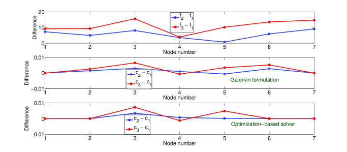
Figure 1. This figure illustrates the violation of the comparison principle by the optimization-based solver. Note that the Galerkin formulation also violates the comparison principle. The problem is a one-dimensional problem with homogeneous Dirichlet boundary conditions. The decay coefficient is taken as $2\times 10^{4}$, the diffusivity coefficient is taken as unity, and the domain is meshed using six linear finite elements. As evident from the figure, we have $\boldsymbol{f}_{3}\succeq\boldsymbol{f}_{2}\succeq\boldsymbol{f}_{1}$ but the obtained numerical solution does not obey $\boldsymbol{c}_{3}\succeq\boldsymbol{c}_{2}\succeq\boldsymbol{c}_{1}$.

3. The methodology does not satisfy the comparison principle. A counterexample is provided in Figure 1. However, if $\boldsymbol{f}_{1}=\eta\boldsymbol{f}_{2}$ with $\eta\geq 0$, then $\boldsymbol{c}_{1}=\eta\boldsymbol{c}_{2}$ under the optimization-based solver.

4. Although a discrete version of the comparison principle does not hold, a unique solution always exists under the optimization-based solver. The existence and the uniqueness of the solution in the discrete setting stems from the results in the convex programming with bounds on the variables. Of course, the proofs from the optimization theory do not require a discrete version of the comparison principle to hold but use alternate approaches from Matrix Algebra and Analysis [69].

5. The solution procedure is nonlinear, as a quadratic programming optimization problem with inequalities is nonlinear.

6. One can employ the consistent capacity matrix that stems from the variational structure of the underling weak formulation. If needed, one can also employ a lumped capacity matrix, which is considered to be a variational crime.

In conclusion, the proposed optimization methodology does not possess a commutative diagram similar to the one given above. But it should be noted that the optimization-based method is the only known methodology that satisfies the non-negative principle and the maximum principle on general computational grids with no additional restrictions on the time step. Some other noteworthy efforts on non-negative solvers for diffusion-type equations are by Le Potier [70] and Lipnikov et al. [71, 72], which have the following attributes:

1. The methodology is based on the finite volume method.

2. The methodology satisfies the non-negative principle on computational grids with triangles. The method does not satisfy the maximum principle.

3. The methodology does not satisfy the comparison principle.

4. The solution procedure is nonlinear, as the collocation points (i.e., the location of the unknown concentrations) in turn depend on the concentration.

5. One can employ only a lumped capacity matrix, which is consistent with the finite volume method. Also, one has to employ the backward Euler time stepping scheme, as any other time stepping scheme can result in an algorithmic failure or can produce negative concentrations.

Some recent finite volume methods [73, 74] and finite difference methods [75] have succeeded in overcoming the aforementioned limitation (ii) (i.e., these methods satisfy maximum principles).

5. NUMERICAL PERFORMANCE OF THE PROPOSED COMPUTATIONAL FRAMEWORK

In this section we shall illustrate the performance of the proposed computational framework for diffusive-reactive systems given by equations (2.6a)–(2.6f). We shall also perform numerical $h$-convergence using hierarchical meshes. We shall solve three representative problems: plume development from a boundary, plume formation due to continuous point source emitters, and decay of a chemically reacting slug. These types of problems have many practical applications. For example, these problems naturally arise from situations in which one may want to regulate/control an induced contaminant in an ecological system, which is often achieved by introducing a suitable chemical or biological species that reacts with the contaminant to form a harmless product. Some specific examples include chemical dispersion methods to control oil spills and airborne contaminants, and usage of bioremediators for regulating industrial emissions into water bodies.

In all the numerical simulations reported in this paper, the resulting convex quadratic programming problems are solved using the MATLAB’s [76] built-in function handler quadprog, which offer robust solvers for solving quadratic programming problems. In particular, we have used the specific algorithm that can be invoked using the interior-point-convex option under quadprog, which is based on the numerical methods presented in references [77, 78, 79]. For further details, see MATLAB’s documentation [76]. The tolerance in the stopping criterion in solving convex quadratic programming is taken as $100\epsilon_{\mathrm{mach}}$, where $\epsilon_{\mathrm{mach}}\approx 2.22\times 10^{-16}$ is the machine precision for a 64-bit machine.

5.1. Numerical $h$-convergence study

We shall use the method of manufactured solutions to perform numerical $h$-convergence. We shall restrict the current study to steady-state response. The computational domain is a rectangle of size $L_{x}\times L_{y}$. The diffusivity tensor for this numerical study is taken as follows:

$$\mathbf{D}(\mathbf{x})=\mathbf{R}\mathbf{D}_{\mathrm{diagonal}}\mathbf{R}^{\mathrm{T}}$$ (5.1)

where

$$\mathbf{R}=\left(\begin{array}[]{cc}\cos(\theta)&-\sin(\theta)\\ \sin(\theta)&\cos(\theta)\\ \end{array}\right)$$ (5.4)

$$\mathbf{D}_{\mathrm{diagonal}}=\left(\begin{array}[]{cc}d_{1}&0\\ 0&d_{2}\\ \end{array}\right)$$ (5.7)

The assumed analytical solutions for $c_{F}(\mathbf{x})$ and $c_{G}(\mathbf{x})$ are taken as follows:

$$c_{F}(\mathbf{x}) =\sin\left(\frac{\pi\mathrm{x}}{2L_{x}}\right)\sin\left(\frac{\pi\mathrm{y}}{2L_{y}}\right)$$ (5.8a)

$$c_{G}(\mathbf{x}) =\cos\left(\frac{\pi\mathrm{x}}{2L_{x}}\right)\cos\left(\frac{\pi\mathrm{y}}{2L_{y}}\right)$$ (5.8b)

where $0\leq\mathrm{x}\leq L_{x}$ and $0\leq\mathrm{y}\leq L_{y}$. Using the above expressions, the source terms, boundary conditions, and expressions for the concentrations of $A$, $B$, and $C$ are in turn calculated. The corresponding volumetric sources for invariants $F$ and $G$ are given as follows:

$$f_{F}(\mathrm{x},\mathrm{y}) =\frac{\pi^{2}}{4}\sin\left(\frac{\pi\mathrm{x}}{2L_{x}}\right)\sin\left(\frac{\pi\mathrm{y}}{2L_{y}}\right)\left(d_{1}\left(\frac{\cos^{2}(\theta)}{L_{x}^{2}}+\frac{\sin^{2}(\theta)}{L_{y}^{2}}\right)+d_{2}\left(\frac{\sin^{2}(\theta)}{L_{x}^{2}}+\frac{\cos^{2}(\theta)}{L_{y}^{2}}\right)\right)$$

$$-\frac{\pi^{2}}{2L_{x}L_{y}}\left(d_{1}-d_{2}\right)\sin(\theta)\cos(\theta)\cos\left(\frac{\pi\mathrm{x}}{2L_{x}}\right)\cos\left(\frac{\pi\mathrm{y}}{2L_{y}}\right)$$ (5.9a)

$$f_{G}(\mathrm{x},\mathrm{y}) =\frac{\pi^{2}}{4}\cos\left(\frac{\pi\mathrm{x}}{2L_{x}}\right)\cos\left(\frac{\pi\mathrm{y}}{2L_{y}}\right)\left(d_{1}\left(\frac{\cos^{2}(\theta)}{L_{x}^{2}}+\frac{\sin^{2}(\theta)}{L_{y}^{2}}\right)+d_{2}\left(\frac{\sin^{2}(\theta)}{L_{x}^{2}}+\frac{\cos^{2}(\theta)}{L_{y}^{2}}\right)\right)$$

$$-\frac{\pi^{2}}{2L_{x}L_{y}}\left(d_{1}-d_{2}\right)\sin(\theta)\cos(\theta)\sin\left(\frac{\pi\mathrm{x}}{2L_{x}}\right)\sin\left(\frac{\pi\mathrm{y}}{2L_{y}}\right)$$ (5.9b)

A pictorial description of the boundary value problem is given in Figure 2. In this paper, we have taken the following values for the parameters to perform the steady-state numerical $h$-convergence:

$$L_{x}=2,\;L_{y}=1,\;\theta=\pi/3,\;d_{1}=1000,\;d_{2}=1,\;n_{A}=2,\;n_{B}=3,\;n_{C}=1$$ (5.10)

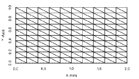
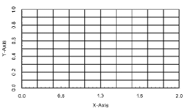
Figure 3. Numerical $h$-convergence study: This figure shows the typical computational meshes (using three-node triangular and four-node quadrilateral elements) employed in the numerical convergence study. Hierarchical meshes are employed in the study. The meshes shown in the figure have $11$ nodes along each side of the domain. Convergence analysis is performed using $11\times 11$, $21\times 21$, $41\times 41$, and $81\times 81$ meshes.

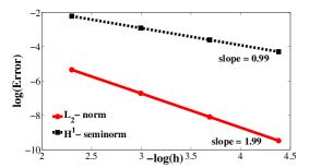
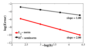
Figure 4. Numerical $h$-convergence study: This figure shows the variation of error in the concentrations of invariants $F$ and $G$ with respect to mesh refinement. The left figure is for three-node triangular element, and the right figure is for four-node quadrilateral element. The error is calculated in both $L_{2}$ norm and $H^{1}$ seminorm. Since the obtained values for the error are identical for both $F$ and $G$, only the error for invariant $F$ is shown in the figure.

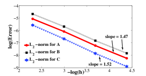
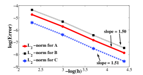
Figure 5. Numerical $h$-convergence study: This figure shows the variation of error in the concentrations of $A$, $B$, and $C$ with respect to mesh refinement. The left figure is for three-node triangular element, and the right figure is for four-node quadrilateral element. It is evident that the numerical solution obtained from the proposed computational framework converges with respect to mesh refinement.

Figure 3 shows the typical computational meshes employed in this study. Figure 4 illustrates the convergence of the concentration of the invariants, and the convergence for the concentrations of the chemical species $A$, $B$, and $C$ is shown in Figure 5. For invariants, we have shown the convergence in both $L_{2}$ norm and $H^{1}$ seminorm. However, for the chemical species $A$, $B$, and $C$, we have shown the convergence only in $L_{2}$ norm as $\mathrm{max}[\cdot]$ operator is non-smooth.

5.2. Plume development from boundary in a reaction tank

The test problem is pictorially described in Figure 6. We restrict the present study to steady-state analysis. The stoichiometric coefficients are taken as $n_{A}=1$, $n_{B}=1$ and $n_{C}=2$. The diffusivity tensor is taken from the subsurface literature [13], and can be written as follows:

$$\mathbf{D}_{\mathrm{subsurface}}(\mathbf{x})=\alpha_{T}\|\mathbf{v}\|\mathbf{I}+\frac{\alpha_{L}-\alpha_{T}}{\|\mathbf{v}\|}\mathbf{v}\otimes\mathbf{v}$$ (5.11)

where $\otimes$ is the tensor product, $\mathbf{v}$ is velocity vector field, and $\alpha_{T}$ and $\alpha_{L}$ are, respectively, transverse and longitudinal diffusivity coefficients. It should be emphasized that we have neglected the advection, and the velocity is used to define the diffusion tensor. The velocity field is defined through a multi-mode stream function, which takes the following form:

$$\psi(\mathrm{x},\mathrm{y})=-\mathrm{y}-\sum_{k=1}^{3}A_{k}\cos\left(\frac{{p}_{k}\pi\mathrm{x}}{L_{x}}-\frac{\pi}{2}\right)\sin\left(\frac{q_{k}\pi\mathrm{y}}{L_{y}}\right)$$ (5.12)

The corresponding components of the velocity are given by

$$\mathrm{v}_{\mathrm{x}}(\mathrm{x},\mathrm{y}) =-\frac{\partial\psi}{\partial\mathrm{y}}=1+\sum_{k=1}^{3}A_{k}\frac{q_{k}\pi}{L_{y}}\cos\left(\frac{p_{k}\pi\mathrm{x}}{L_{x}}-\frac{\pi}{2}\right)\cos\left(\frac{q_{k}\pi\mathrm{y}}{L_{y}}\right)$$ (5.13a)

$$\mathrm{v}_{\mathrm{y}}(\mathrm{x},\mathrm{y}) =+\frac{\partial\psi}{\partial\mathrm{x}}=\sum_{k=1}^{3}A_{k}\frac{p_{k}\pi}{L_{x}}\sin\left(\frac{p_{k}\pi\mathrm{x}}{L_{x}}-\frac{\pi}{2}\right)\sin\left(\frac{q_{k}\pi\mathrm{y}}{L_{y}}\right)$$ (5.13b)

It is noteworthy that the above velocity vector field is solenoidal (i.e., $\mathrm{div}[\mathbf{v}]=0$). Although realistic aquifers exhibit spatial variability on a hierarchy of scales, periodic or quasi-periodic models similar to the one outlined above (given by equations (5.11)–(5.13)) have often been used due to their simplicity [80, 81].

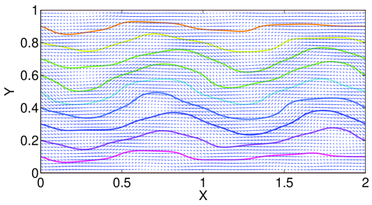
Figure 7. This figure shows the contours of the multi-mode stream function given by equation (5.12), and corresponding vector field given by equation (5.13). It should be emphasized that the velocity should not be associated with the advection velocity, as advection is neglected in this paper. Herein, the velocity (given by equation (5.13)) should be interpreted as the principal directions (or eigenvectors) of the diffusivity tensor (which is given by equation (5.11)). Since the streamlines do not intersect, the nature of the vector fields can provide insights on the plume of the reactants and the product.

In this paper we shall take $(L_{x},L_{y})=(2,1)$, $(p_{1},p_{2},p_{3})=(4,5,10)$, $(q_{1},q_{2},q_{3})=(1,5,10)$, $(A_{1},A_{2},A_{3})=(0.08,0.02,0.01)$, and $(\alpha_{L},\alpha_{T})=(1,0.0001)$. The contours of the stream function, and the corresponding velocity vector field are shown in Figure 7. The computational domain is meshed using four-node quadrilateral elements. The numerical simulation is carried out on various structured meshes with XSeed and YSeed ranging from 97 to 259, where XSeed and YSeed are, respectively, the number of nodes along the x-direction and y-direction. That is, a structured mesh with XSeed = YSeed = 259 has over 67,000 unknown nodal concentrations.

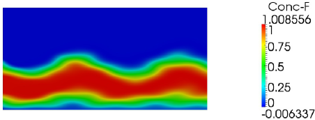
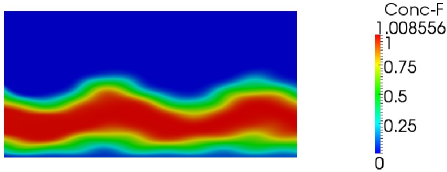
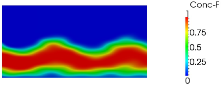
Figure 8. Plume formation from boundary in a reaction tank: This figure shows the contours of the invariant $F$ obtained using the Galerkin formulation (top figure), the clipping procedure (middle figure), and the proposed computational framework (bottom figure). The concentration of the invariant $F$ should be between $0$ and $1$. The Galerkin formulation violates the non-negative constraint and the maximum principle. On the other hand, by explicitly enforcing the lower and upper bounds, the proposed computational framework satisfies the non-negative constraint and the maximum principle. However, it is noteworthy that the contours of the invariant $F$ under the Galerkin formulation, the clipping procedure and the proposed computational framework all look similar. This is not the case with the contours of the product $C$ (see Figure 12).

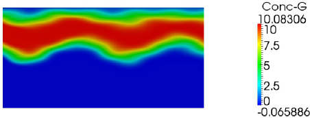
Figure 9. Plume formation from boundary in a reaction tank: This figure shows the contours of the invariant $G$ obtained using the Galerkin formulation (top figure), the clipping procedure (middle figure), and the proposed computational framework (bottom figure). The concentration of the invariant $G$ should be between $0$ and $10$. The Galerkin formulation violates the non-negative constraint and the maximum principle. On the other hand, by explicitly enforcing the lower and upper bounds, the proposed computational framework satisfies the non-negative constraint and the maximum principle. However, it is noteworthy that the contours of the invariant $G$ under the Galerkin formulation, the clipping procedure and the proposed computational framework all look similar. This is not the case with the contours of the product $C$ (see Figure 12).

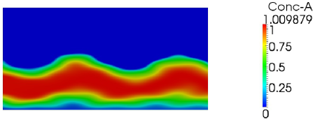
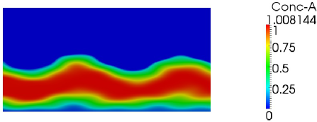
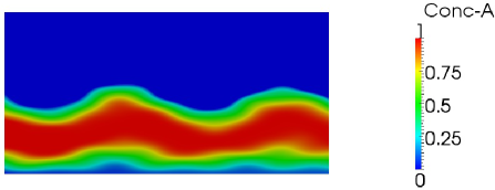
Figure 10. Plume formation from boundary in a reaction tank: This figure shows the contours of the reactant $A$ obtained using the Galerkin formulation (top figure), the clipping procedure (middle figure), and the proposed computational framework (bottom figure). The concentration of the reactant $A$ should be less than or equal to $1$. The Galerkin formulation violates the maximum principle. On the other hand, the proposed computational framework satisfies the upper bound due to the maximum principle. However, it is noteworthy that the contours of the reactant $A$ under the Galerkin formulation, the clipping procedure and the proposed computational framework all look similar. This is not the case with the contours of the product $C$ (see Figure 12).

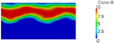
Figure 11. Plume formation from boundary in a reaction tank: This figure shows the contours of the reactant $B$ obtained using the Galerkin formulation (top figure), the clipping procedure (middle figure), and the proposed computational framework (bottom figure). The concentration of the reactant $B$ should be less than or equal to $10$. The Galerkin formulation violates the maximum principle. On the other hand, the proposed computational framework satisfies the upper bound due to the maximum principle. However, it is noteworthy that the contours of the reactant $B$ under the Galerkin formulation, the clipping procedure and the proposed computational framework all look similar. This is not the case with the contours of the product $C$ (see Figure 12).

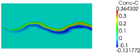
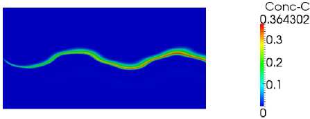
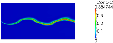
Figure 12. Plume formation from boundary in a reaction tank: This figure shows the contours of the concentration of the product $C$ obtained using the Galerkin formulation (top figure), the clipping procedure (middle figure), and the proposed computational framework (bottom figure). Mathematically, the concentration of the product $C$ should be non-negative. There is no upper bound on the concentration of the product due to the maximum principle, as there is a source for the product $C$ due to the underlying reaction. As one can see from the figure, the Galerkin formulation violates the non-negative constraint. On the other hand, the proposed computational framework satisfies the non-negative constraint for the concentration of the product $C$. More importantly, the contours of the product under the Galerkin formulation, the clipping procedure and the proposed computational framework differ considerably. Using this figure, one can draw an important conclusion of the paper: A small violation of the non-negative constraint and the maximum principle in the calculation of the invariants can result in significant errors in the concentration of the product for diffusive-reactive systems.

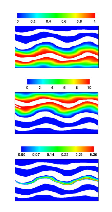
Figure 13. Plume formation from boundary in a reaction tank: This figure shows the contours of invariant $F$ (top figure), invariant $G$ (middle figure), and product $C$ (bottom figure) under the Galerkin formulation. For the invariant $F$, the concentrations outside the interval $[0,1]$ are cut-off, and for the invariant $G$ the concentrations outside $[0,10]$ are cut-off. For the product $C$, the concentrations below zero are cut-off. The lower bounds are due to the non-negative constraint, and the upper bounds are due to the maximum principle. The regions with cut-off concentration values are indicated in white color. It is evident that the Galerkin formulation violated the bounds in significant portions of the computational domain.

The values for prescribed concentrations on the boundary are taken as $c_{A}^{\mathrm{p}}=1$ and $c_{B}^{\mathrm{p}}=10$. Figures 8–12 compare the contours of the concentrations of the invariants, reactants and product under the Galerkin formulation, the clipping procedure and the proposed non-negative formulation. Figure 13 shows the regions in the domain that have violated the lower and upper bounds on the concentrations of the invariants and the product under the Galerkin formulation. To provide more quantitative inference on the violations, the variation of the concentration of the product along two sections given by $\mathrm{y}=0.45$ and $\mathrm{x}=1.75$ is plotted in Figure 14.

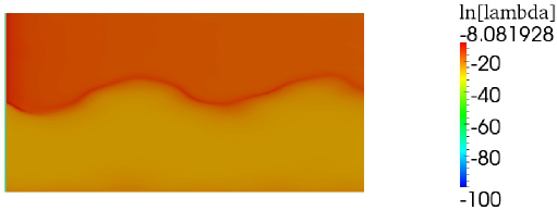
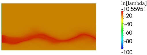
Figure 17. Plume formation from boundary in a reaction tank: This figure shows the contours of the natural logarithm of the Lagrange multipliers corresponding to the lower bound constraints (top) and the upper bound constraints (bottom) for the invariant $F$. The proposed computational framework is employed, which solves a quadratic programming problems to obtain the concentration of invariant $F$. It should be noted that the Lagrange multipliers will always be non-negative, and hence the natural logarithm of the Lagrange multipliers will be (extended) real numbers. For visualization purposes, we have set the natural logarithm of zero to be $-100$.

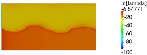
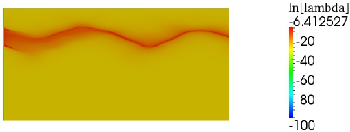
Figure 18. Plume formation from boundary in a reaction tank: This figure shows the contours of the natural logarithm of the Lagrange multipliers corresponding to the lower bound constraints (top) and the upper bound constraints (bottom) for the invariant $G$. The proposed computational framework is employed, which solves a quadratic programming problems to obtain the concentration of invariant $G$. It should be noted that the Lagrange multipliers will always be non-negative, and hence the natural logarithm of the Lagrange multipliers will be (extended) real numbers. For visualization purposes, we have set the natural logarithm of zero to be $-100$.

Figures 15 and 16 show the variation of the total concentration, $\int c(\mathrm{x},\mathrm{y})\;\mathrm{d}\mathrm{y}$, along the x-direction for the invariants and the product. The total concentration for a given cross-section is a useful measure in the studies on reactive-transport. The results are shown for various mesh refinements, and the Galerkin formulation predicts unphysical negative values even for this important global measure. On the other hand, the proposed computational framework predicts physically meaningful for the considered measure. Figures 17 and 18 show the contours of the Lagrange multipliers in solving quadratic programming problems to obtain the invariants $F$ and $G$. The Lagrange multipliers arise due to the enforcement of the lower and upper bounds due to the non-negative constraint and the maximum principle in calculating the invariants. It should be noted that, based on the Karush-Kuhn-Tucker results in the theory of optimization, the Lagrange multipliers are non-negative [69].

5.3. Plume formation due to multiple stationary point sources

The problem is pictorially described in Figure 19. The following rotated heterogeneous diffusivity tensor is employed:

$$\mathbf{D}(\mathbf{x})=\mathbf{R}\mathbf{D}_{0}(\mathbf{x)}\mathbf{R}^{\mathrm{T}}$$ (5.14)

where $\mathbf{D}_{0}(\mathbf{x})$ is

$$\mathbf{D}_{0}(\mathbf{x})=\left(\begin{array}[]{cc}\mathrm{y}^{2}+\epsilon\mathrm{x}^{2}&-(1-\epsilon)\mathrm{x}\mathrm{y}\\ -(1-\epsilon)\mathrm{x}\mathrm{y}&\epsilon\mathrm{y}^{2}+\mathrm{x}^{2}\\ \end{array}\right)$$ (5.17)

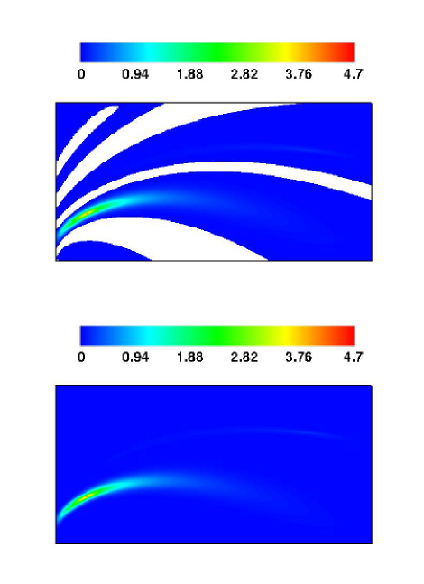
Figure 20. Plume formation due to multiple stationary point sources: This figure shows the steady-state contours of concentration of the invariant $F$ under the Galerkin formulation (top figure), and the non-negative formulation (bottom figure). The minimum and maximum concentrations of $F$ under the Galerkin formulation are respectively $-0.0498$ and $4.7100$, and the corresponding values under the non-negative formulation are respectively $0$ and $4.7088$. The rotated heterogeneous diffusivity tensor is employed in the numerical simulation. The results are generated using $201\times 201$ structured mesh using four-node quadrilateral elements. The regions with negative concentration are indicated in white color.

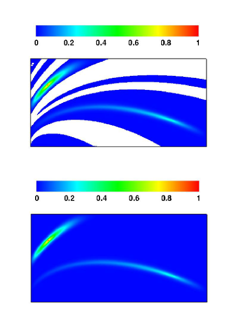
Figure 21. Plume formation due to multiple stationary point sources: This figure shows the steady-state contours of concentration of the invariant $G$ under the Galerkin formulation (top figure), and the non-negative formulation (bottom figure). The minimum and maximum concentrations of $G$ under the Galerkin formulation are respectively $-0.0158$ and $0.9977$, and the corresponding values under the non-negative formulation are respectively $0$ and $0.9969$. The rotated heterogeneous diffusivity tensor is employed in the numerical simulation. The results are generated using $201\times 201$ structured mesh using four-node quadrilateral elements. The regions with negative concentration are indicated in white color.

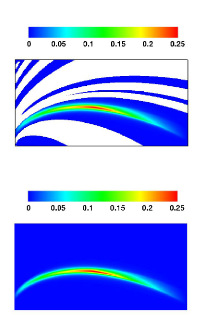
Figure 22. Plume formation due to multiple stationary point sources: This figure shows the steady-state contours of concentration of product $C$ under the Galerkin formulation (top figure), and the non-negative formulation (bottom figure). The minimum and maximum concentrations of $C$ under the Galerkin formulation are respectively $-0.0996$ and $0.2560$, and the corresponding values under the non-negative formulation are respectively $0$ and $0.2564$. The rotated heterogeneous diffusivity tensor is employed in the numerical simulation. The results are generated using $201\times 201$ structured mesh using four-node quadrilateral elements. The regions with negative concentration are indicated in white color.

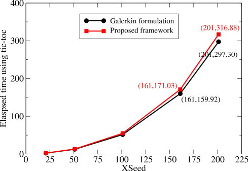
Figure 24. Plume formation due to multiple stationary point sources: This figure compares the CPU timing of the Galerkin formulation and the proposed computational framework. Note that XSeed denotes the number of nodes along the x-direction, and the same number of nodes are employed in the y-direction. In other words, a mesh with XSeed = YSeed = 201 will have over 40,000 total number of nodes. For each node, we have 5 unknowns – two invariants, two reactants, and the product. Note that we have employed MATLAB’s interior-point-convex algorithm to solve the resulting quadratic programming problems. Each point is generated by taking the average of five simulations.

and the rotation tensor is same as before (given by equation (5.4)) with angle $\theta=\pi/3$. For this problem, the parameter $\epsilon$ is taken as $0.001$. The stoichiometry coefficients are taken to be $n_{A}=1$, $n_{B}=1$ and $n_{C}=2$. Figures 20–22 show the contours of the concentrations of the invariants and the product under the Galerkin formulation and the proposed computational framework. Figure 23 shows the variation of the integrated concentration of the product with respect to $\mathrm{y}$ (i.e., $\int c(\mathrm{x},\mathrm{y})\;\mathrm{d}\mathrm{y}$) along $\mathrm{x}$, and the Galerkin formulation dramatically predicts negative values even for this average. Table 1 shows that small violations in the non-negative constraint for invariants can lead to bigger violations in the non-negative constraint for the product $C$. Figure 24 compares the CPU time taken by the Galerkin formulation and the proposed computational framework. Even for a mesh with more than 40,000 nodes, the CPU time taken by the proposed framework is only 1.07 times the CPU time taken by the Galerkin formulation. For this mesh, 50.51% of the nodes have violated the non-negative constraint for the product under the Galerkin formulation. On the other hand, the nodal concentrations of the product under the proposed computational framework are physically meaningful non-negative values.

Table 1. Plume formulation due to multiple stationary point sources: This table shows the minimum concentration, maximum concentration, and % of nodes violated the non-negative constraint under the Galerkin formulation. The values clearly indicate that small violations in meeting the non-negative constraint for invariants can result in much bigger violation of the non-negative constraint for the product. It is important to note that Ciarlet and Raviart [82] have shown that the Galerkin single-field formulation, in general, does not converge uniformly for diffusion-type equations. That is, the numerical solutions under the Galerkin formulation for diffusion-type equations converge in $L_{2}$ norm but need not converge in $L^{\infty}$ norm.

Mesh	Invariant F		Invariant G
	$\frac{\mbox{Min. conc.}}{\mbox{Max. conc.}}\times 100$	nodes violated	$\frac{\mbox{Min. conc.}}{\mbox{Max. conc.}}\times 100$	nodes violated
$21\times 21$	$\frac{-1.50\times 10^{-3}}{1.42\times 10^{0}}\times 100=-0.11\%$	8.62%	$\frac{-2.07\times 10^{-3}}{3.00\times 10^{-1}}\times 100=-0.69\%$	23.36%
$51\times 51$	$\frac{-1.38\times 10^{-2}}{2.37\times 10^{0}}\times 100=-0.58\%$	24.14%	$\frac{-8.54\times 10^{-3}}{4.99\times 10^{-1}}\times 100=-1.71\%$	43.71%
$101\times 101$	$\frac{-3.13\times 10^{-2}}{3.38\times 10^{0}}\times 100=-0.93\%$	25.30%	$\frac{-1.31\times 10^{-2}}{7.11\times 10^{-1}}\times 100=-1.84\%$	46.53%
$161\times 161$	$\frac{-4.45\times 10^{-2}}{4.24\times 10^{0}}\times 100=-1.05\%$	25.77%	$\frac{-1.52\times 10^{-2}}{8.96\times 10^{-1}}\times 100=-1.70\%$	45.20%
$201\times 201$	$\frac{-4.98\times 10^{-2}}{4.71\times 10^{0}}\times 100=-1.06\%$	27.29%	$\frac{-1.58\times 10^{-2}}{9.98\times 10^{-1}}\times 100=-1.58\%$	40.83%

Mesh	Product C
	$\frac{\mbox{Min. conc.}}{\mbox{Max. conc.}}\times 100$	nodes violated
$21\times 21$	$\frac{-4.13\times 10^{-3}}{1.22\times 10^{-1}}\times 100=-3.38\%$	31.29%
$51\times 51$	$\frac{-2.75\times 10^{-3}}{1.83\times 10^{-1}}\times 100=-15.05\%$	53.94%
$101\times 101$	$\frac{-6.25\times 10^{-2}}{2.26\times 10^{-1}}\times 100=-27.70\%$	51.02%
$161\times 161$	$\frac{-8.90\times 10^{-2}}{2.48\times 10^{-1}}\times 100=-35.93\%$	54.94%
$201\times 201$	$\frac{-9.96\times 10^{-2}}{2.56\times 10^{-1}}\times 100=-38.90\%$	50.51%

5.4. Diffusion and reaction of an initial slug

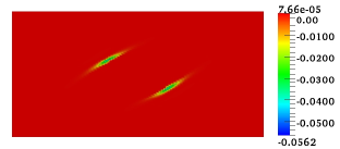
(a) $t=0.05$

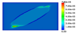
(b) $t=0.05$

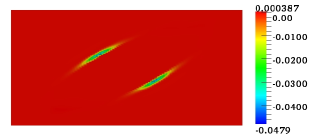
(c) $t=0.1$

(d) $t=0.1$

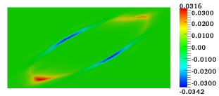
(e) $t=0.5$

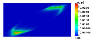
(f) $t=0.5$

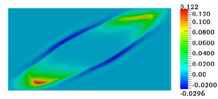
(g) $t=1.0$

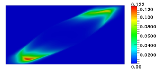
(h) $t=1.0$

Figure 26. Diffusion and reaction of an initial slug: This figure shows the contours of the concentration of the product $C$ under the Galerkin single-field formulation (left) and proposed numerical framewotk (right) at various time levels. The time step is taken as $\Delta t=0.05\;\mathrm{s}$. It is evident from above figures that the Galerkin single-field formulation violated the non-negative constraint, whereas the proposed numerical framework produced physically meaningful values for concentration of the product $C$.

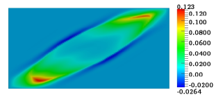
(a) $t=1.0$

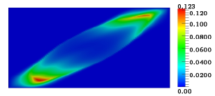
(b) $t=1.0$

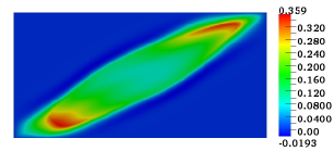
(c) $t=5.0$

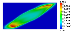
(d) $t=5.0$

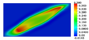
(e) $t=10.0$

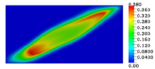
(f) $t=10.0$

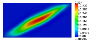
(g) $t=20.0$

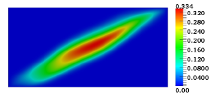
(h) $t=20.0$

Figure 27. Diffusion and reaction of an initial slug: This figure shows the contours of the concentration of the product $C$ under the Galerkin single-field formulation (left) and the proposed numerical framework (right) at various time levels. A larger time step of $\Delta t=1.0\;\mathrm{s}$ is employed. Again, the Galerkin single-field formulation violated the non-negative constraint, and the proposed numerical framework produced physically meaningful solutions.

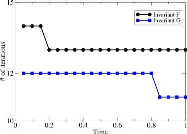
Figure 28. Diffusion and reaction of an initial slug: This figure shows the number of iterations taken by the quadratic programming solver at each time level in obtaining the concentrations for the invariants $F$ and $G$. The time step is taken as $\Delta t=0.05\;\mathrm{s}$.

The test problem is pictorially described in Figure 25. The initial conditions within the reaction slug are assumed to be $c_{A}^{0}=10$, $c_{B}^{0}=0$, and $c_{C}^{0}=0$. In the other parts of the rectangular domain we have $c_{A}^{0}=c_{B}^{0}=c_{C}^{0}=0$. The boundary conditions for the chemical species on the rectangular domain are assumed to be $c_{A}^{\mathrm{p}}=0$, $c_{B}^{\mathrm{p}}=1-\mathrm{e}^{-t}$, and $c_{C}^{\mathrm{p}}=0$. The problem is solved within the time interval $t\in[0,1]$. The diffusivity tensor within the domain is taken as $\mathbf{D}(\mathbf{x})=\mathbf{R}\mathbf{D}_{\mathrm{subsurface}}\mathbf{R}^{\mathrm{T}}$ with $\theta=\frac{\pi}{6}$. The stoichiometric coefficients are $n_{A}=2$, $n_{B}=2$, and $n_{C}=1$. Numerical simulations are performed using structured mesh with $101$ nodes along each side of the domain using four-node quadrilateral elements. The volumetric source of each species $A$, $B$, and $C$ is equal to zero inside the rectangular domain. Two different time steps are employed in the numerical simulations: $\Delta t=0.05\;\mathrm{s}$ and $\Delta t=1.0\;\mathrm{s}$. Figures 26 and 27 compare the concentrations of the product $C$ for these time steps under the Galerkin single-field formulation and the proposed numerical framework. As evident from these figures, even for this transient problem, the proposed numerical framework produced physically meaningful non-negative values for the concentration of the product at all time levels. The violation of the non-negative constraint under the Galerkin single-field formulation is greater for smaller time steps and for smaller time levels. Figure 28 shows the number of iterations taken by the quadratic programming solver at each time level to obtain concentrations of the invariants $F$ and $G$. For this transient problem, the CPU times taken by the proposed computational framework and the Galerkin formulation are $1516.83$ and $1486.19$. That is, the computational overhead of the proposed computational framework is $2\%$ when compared with the Galerkin formulation. The elapsed CPU time is measured using MATLAB’s built-in tic-toc feature.

6. CLOSURE

We have presented a robust and computationally efficient non-negative framework for fast bimolecular diffusive-reactive systems. We have rewritten the governing equations for the concentration of reactants and product in terms of invariants which are unaffected by the underlying reaction. Because of this algebraic transformation, instead of solving three coupled (nonlinear) diffusion-reaction equations, we need to solve only two uncoupled linear diffusion equations. This will considerably decrease the computational cost and also avoid numerical challenges due to nonlinear terms. One of the main findings of this paper is that a small violation of the non-negative constraint and maximum principle in the calculation of invariants can result in bigger errors in the prediction of the concentration of the product.

Using several numerical experiments, it has been shown that the standard single-field formulation (which is also known as the Galerkin formulation) gives unphysical negative values for the concentration of the invariants, reactants, and the product. The formulation even gives unphysical negative value for the average of the concentration of the product, which is a useful measure in the prediction of the fate of transport of chemical species. It is also shown that the clipping procedure (which is considered as a variational crime) is not a viable fix to obtain the non-negative concentrations, and does not give accurate results for diffusive-reactive systems. On the other hand, the proposed computational framework provided accurate results, and in all cases the framework provided non-negative values for the concentrations of the chemical species. The proposed computational framework can serve as a robust simulator for anisotropic heterogeneous geomodels. A next logical step is to extend the proposed computational framework to slow reactions, and to more complicated reactions.

\psfrag{F}{Volumetric source of invariant-$F$ is given by equation \ref{Eqn:Volumetric_Source_Invariant_F}}\psfrag{G}{Volumetric source of invariant-$G$ is given by equation \ref{Eqn:Volumetric_Source_Invariant_G}}\psfrag{xo}{$\mathbf{x}_{\mathrm{origin}}$}\psfrag{Lx}{$L_{x}$}\psfrag{Ly}{\rotatebox{-90.0}{$L_{y}$}}\psfrag{BC1}{\rotatebox{90.0}{$c_{F}^{\mathrm{p}}(\mathbf{x})=0$ , $c_{G}^{\mathrm{p}}(\mathbf{x})=\cos\left(\frac{\pi y}{2L_{y}}\right)$}}\psfrag{BC2}{$c_{F}^{\mathrm{p}}(\mathbf{x})=\sin\left(\frac{\pi x}{2L_{x}}\right)$ , $c_{G}^{\mathrm{p}}(\mathbf{x})=0$}\psfrag{BC3}{\rotatebox{-90.0}{$c_{F}^{\mathrm{p}}(\mathbf{x})=\sin\left(\frac{\pi y}{2L_{y}}\right)$ , $c_{G}^{\mathrm{p}}(\mathbf{x})=0$}}\psfrag{BC4}{$c_{F}^{\mathrm{p}}(\mathbf{x})=0$ , $c_{G}^{\mathrm{p}}(\mathbf{x})=\cos\left(\frac{\pi x}{2L_{x}}\right)$}\includegraphics[scale={0.9}]{Figures/Convergence_Study_SteadyState.eps}

Figure 2. Numerical $h$-convergence study: A pictorial description of the boundary value problem. The computational domain is a rectangle with origin at $\mathbf{x}_{\mathrm{origin}}=(0,0)$. The length and width of the rectangular domain is $L_{x}=2$ and $L_{y}=1$. The volumetric sources for invariants $F$ and $G$ are prescribed. The Dirichlet boundary conditions $c_{F}^{\mathrm{p}}(\mathbf{x})$ and $c_{G}^{\mathrm{p}}(\mathbf{x})$ are prescribed directly by evaluating the expressions given by equations (5.8a) and (5.8b) on the boundary.

\psfrag{A}{$A$}\psfrag{B}{$B$}\psfrag{P}{$\mathrm{P}$}\psfrag{Q}{$\mathrm{Q}$}\psfrag{cAp}{$c_{A}^{\mathrm{p}}$}\psfrag{cBp}{$c_{B}^{\mathrm{p}}$}\psfrag{Lx}{$L_{x}$}\psfrag{Ly}{$L_{y}$}\psfrag{Ly6}{$L_{y}/6$}\psfrag{x}{$\boldsymbol{x}$}\psfrag{y}{$\boldsymbol{y}$}\psfrag{zero}{zero flux}\psfrag{D}{Dirichlet BC}\includegraphics[scale={0.6}]{Figures/Reaction_tank.eps}

Figure 6. Plume development from boundary in a reaction tank: A pictorial description of boundary value problem. The computational domain is a rectangle with reactants $A$ and $B$ are pumped on the left face of the domain, which are modeled as Dirichlet boundary conditions. On the remaining faces of the domain, no flux (i.e., Neumann) boundary condition is applied. Dirichlet boundary conditions for $A$ and $B$ are also indicated in the figure.

\psfrag{cC_y_dot45}{$c_{C}(\mathrm{x},\mathrm{y}=0.45)$}\psfrag{cC_x_1dot75}{$c_{C}(\mathrm{x}=1.75,\mathrm{y})$}\psfrag{x}{$\mathrm{x}$}\psfrag{y}{$\mathrm{y}$}\includegraphics[clip,scale={0.45}]{Figures/Plume_subsurface_cC_at_y_dot45.eps}

\psfrag{cC_y_dot45}{$c_{C}(\mathrm{x},\mathrm{y}=0.45)$}\psfrag{cC_x_1dot75}{$c_{C}(\mathrm{x}=1.75,\mathrm{y})$}\psfrag{x}{$\mathrm{x}$}\psfrag{y}{$\mathrm{y}$}\includegraphics[clip,scale={0.45}]{Figures/Plume_subsurface_cC_at_x_1dot75.eps}

Figure 14. Plume formation from boundary in a reaction tank: This figure shows the variation of the concentration of the product at $\mathrm{y}=0.45$ (top figure) and $\mathrm{x}=1.75$ (bottom figure). The Galerkin formulation produces negative concentrations for the product that is extended over significant region, and the violation is not mere numerical noise. It should also be noted the concentration of the product under the clipping procedure is different from that of the proposed computational framework.

\psfrag{intcF}{$\int c_{F}(\mathrm{x},\mathrm{y})\;\mathrm{dy}$}\psfrag{intcG}{$\int c_{G}(\mathrm{x},\mathrm{y})\;\mathrm{dy}$}\psfrag{x}{$\mathrm{x}$}\includegraphics[clip,scale={0.45}]{Figures/Plume_subsurface_intcF.eps}

\psfrag{intcF}{$\int c_{F}(\mathrm{x},\mathrm{y})\;\mathrm{dy}$}\psfrag{intcG}{$\int c_{G}(\mathrm{x},\mathrm{y})\;\mathrm{dy}$}\psfrag{x}{$\mathrm{x}$}\includegraphics[clip,scale={0.45}]{Figures/Plume_subsurface_intcG.eps}

Figure 15. Plume formation from boundary in a reaction tank: This figure shows the variation of integrated concentration of the invariants $F$ and $G$ with respect to $\mathrm{y}$ along x (i.e., the variations of $\int c_{F}(\mathrm{x},\mathrm{y})\;\mathrm{dy}$ and $\int c_{G}(\mathrm{x},\mathrm{y})\;\mathrm{dy}$ along $\mathrm{x}$) for various meshes using the Galerkin formulation, and the proposed computational framework. The results obtained under the clipping procedure are almost the same as that of the Galerkin formulation and the proposed computational framework, and hence not shown in the figure.

\psfrag{intcC}{$\int c_{C}(\mathrm{x},\mathrm{y})\;\mathrm{dy}$}\psfrag{x}{$\mathrm{x}$}\includegraphics[clip,scale={0.45}]{Figures/Plume_subsurface_intcC.eps}

Figure 16. Plume formation from boundary in a reaction tank: This figure shows the variation of integrated concentration of the product $C$ with respect to $\mathrm{y}$ along x (i.e., the variation of $\int c_{C}(\mathrm{x},\mathrm{y})\;\mathrm{dy}$ along $\mathrm{x}$) for various meshes using the Galerkin formulation, the clipping procedure, and the proposed computational framework. This figure clearly shows that the Galerkin formulation predicts unphysical negative values even for average quantities. In particular, the Galerkin formulation predicts negative values for the cross-sectional total concentration of the product for significant portions along the $\mathrm{x}$-direction even on fine computational grids.

\psfrag{A1}{$A\,,\,f^{1}_{A}$}\psfrag{A2}{$A\,,\,f^{2}_{A}$}\psfrag{B1}{$B\,,\,f^{1}_{B}$}\psfrag{B2}{$B\,,\,f^{2}_{B}$}\psfrag{xo}{$\mathbf{x}_{\mathrm{origin}}$}\psfrag{x1}{$\mathbf{x}_{1}=(\mathrm{x}_{1},\mathrm{y}_{1})$}\psfrag{x2}{$\mathbf{x}_{2}=(\mathrm{x}_{2},\mathrm{y}_{2})$}\psfrag{x3}{$\mathbf{x}_{3}=(\mathrm{x}_{3},\mathrm{y}_{3})$}\psfrag{x4}{$\mathbf{x}_{4}=(\mathrm{x}_{4},\mathrm{y}_{4})$}\psfrag{Lx}{$L_{x}$}\psfrag{Ly}{\rotatebox{-90.0}{$L_{y}$}}\psfrag{BC1}{\rotatebox{90.0}{$c_{A}^{\mathrm{p}}(\mathbf{x})=0$ , $c_{B}^{\mathrm{p}}(\mathbf{x})=0$, $c_{C}^{\mathrm{p}}(\mathbf{x})=0$}}\psfrag{BC2}{$c_{A}^{\mathrm{p}}(\mathbf{x})=0$ , $c_{B}^{\mathrm{p}}(\mathbf{x})=0$, $c_{C}^{\mathrm{p}}(\mathbf{x})=0$}\psfrag{BC3}{\rotatebox{-90.0}{$c_{A}^{\mathrm{p}}(\mathbf{x})=0$ , $c_{B}^{\mathrm{p}}(\mathbf{x})=0$, $c_{C}^{\mathrm{p}}(\mathbf{x})=0$}}\psfrag{BC4}{$c_{A}^{\mathrm{p}}(\mathbf{x})=0$ , $c_{B}^{\mathrm{p}}(\mathbf{x})=0$, $c_{C}^{\mathrm{p}}(\mathbf{x})=0$}\includegraphics[scale={0.9}]{Figures/Plume_Numerical_Convergence.eps}

Figure 19. Plume formation due to multiple stationary point sources: A pictorial description of boundary value problem. The computational domain is a rectangle with origin at $\mathbf{x}_{\mathrm{origin}}=(0,0)$. The length and width of the rectangular domain is $L_{x}=2$ and $L_{y}=1$. Continuous point sources of chemical species $A$ and $B$ are located at $\mathbf{x}_{1}=(0.2,0.3)$, $\mathbf{x}_{2}=(1.6,0.3)$, $\mathbf{x}_{3}=(1.6,0.7)$, and $\mathbf{x}_{4}=(0.2,0.7)$ release reactants at a constant rate of $f^{1}_{A}=0.1$, $f^{2}_{A}=0.05$, $f^{1}_{B}=0.1$, and $f^{2}_{B}=0.1$ moles. The Dirichlet boundary conditions $c_{A}^{\mathrm{p}}(\mathbf{x})$ , $c_{B}^{\mathrm{p}}(\mathbf{x})$, and $c_{C}^{\mathrm{p}}(\mathbf{x})$ are prescribed to be zero on the boundary.

\psfrag{intcC}{$\int c_{C}(\mathrm{x},\mathrm{y})\;\mathrm{d}\mathrm{y}$}\includegraphics[clip,scale={0.5}]{Figures/Plume_PointSources_heterogeneous_rotation_intcC.eps}

Figure 23. Plume formation due to multiple stationary point sources: This figure shows the variation of integrated steady-state concentration of the product $C$ with respect to $\mathrm{y}$ along x (i.e., the variation of $\int c_{C}(\mathrm{x},\mathrm{y})\;\mathrm{dy}$ along $\mathrm{x}$) for various meshes using the Galerkin formulation and the proposed computational framework. Three different structured meshes using four-node quadrilateral elements are employed, which are indicated as $101\times 101$, $161\times 161$ and $201\times 201$. The rotated heterogeneous diffusivity tensor is employed in the numerical simulation.

\psfrag{A}{$A\,,\,c_{A}^{0}$}\psfrag{B1}{$A\,,\,c_{A}^{0}=0$}\psfrag{B2}{$B\,,\,c_{B}^{0}$}\psfrag{IC}{Initial conditions for chemical species $A$ and $B$}\psfrag{xo}{$\mathbf{x}_{\mathrm{origin}}$}\psfrag{xs}{$\mathbf{x}_{\mathrm{slug}}$}\psfrag{Lx}{$L_{x}$}\psfrag{Ly}{\rotatebox{-90.0}{$L_{y}$}}\psfrag{dx}{$d_{x}$}\psfrag{dy}{\rotatebox{-90.0}{$d_{y}$}}\psfrag{BC1}{\rotatebox{90.0}{$c_{A}^{\mathrm{p}}=0$ , $c_{B}^{\mathrm{p}}$}}\psfrag{BC2}{$c_{A}^{\mathrm{p}}=0$ , $c_{B}^{\mathrm{p}}$}\psfrag{BC3}{\rotatebox{-90.0}{$c_{A}^{\mathrm{p}}=0$ , $c_{B}^{\mathrm{p}}$}}\psfrag{BC4}{$c_{A}^{\mathrm{p}}=0$ , $c_{B}^{\mathrm{p}}$}\includegraphics[scale={0.9}]{Figures/Plume_Slug.eps}

Figure 25. Diffusion and reaction of an initial slug: A pictorial description of the initial boundary value problem. The slug of dimensions $d_{x}=2$ , $d_{y}=1$ is located at $\mathbf{x}_{\mathrm{slug}}=(4,2)$ in the rectangular domain of length $L_{x}=10$ and breadth $L_{y}=5$.

References

- [1] P. L. McCarty and C. S. Criddle. Chemical and biological processes: The need for mixing. In P. K. Kitanidis and P. L. McCarty, editors, Delivery and Mixing in the Subsurface: Processes and Design Principles for In Situ Remediation, pages 7–52. Springer, 2012.
- [2] M. Dentz, T. Le Borgne, A. Englert, and B. Bijeljic. Mixing, spreading and reaction in heterogeneous media: A brief review. Journal of Contaminant Hydrology, 120-121:1–17, 2011.
- [3] O. A. Cirpka and A. J. Valocchi. Two-dimensional concentration distribution for mixing controlled bioreactive transport in steady state. Advances in Water Resources, 30:1668–1679, 2007.
- [4] T. Arbogast. Numerical subgrid upscaling of two-phase flow in porous media. In Z. Chen, R. E. Ewing, and Z.-C. Shi, editors, Numerical Treatment of Multiphase Flows in Porous Media, volume 552 of Lecture Notes in Physics, pages 35–49, Springer-Verlag, Berlin, 2000.
- [5] Z. Chen and T. Y. Hou. A mixed multiscale finite element method for elliptic problems with oscillating coefficients. Mathematics of Computation, 72:541–576, 2003.
- [6] J. E. Aarnes. On the use of a mixed multiscale finite element method for greater flexibility and increased speed or improved accuracy in reservoir simulation. Multiscale Modeling & Simulation, 2:421–439, 2004.
- [7] J. E. Aarnes, V. Kippe, and K.-A. Lie. Mixed multiscale finite elements and streamline methods for reservoir simulation of large geomodels. Advances in Water Resources, 28:257–271, 2005.
- [8] J. D. Murray. Mathematical Biology. Springer-Verlag, New York, USA, 1993.
- [9] M. Farkas. Dynamical Models in Biology. Academic Press, San Diego, USA, 2001.
- [10] I. R. Epstein and J. A. Pojman. An Introduction to Nonlinear Chemical Dynamics. Oxford University Press, New York, USA, 1998.
- [11] P. Gray and S. K. Scott. Chemical Oscillations and Instabilities. Oxford University Press, Oxford, UK, 1994.
- [12] D. Walgraef. Spatio-Temporal Pattern Formation. Springer-Verlag, New York, USA, 1997.
- [13] G. F. Pinder and M. A. Celia. Subsurface Hydrology. John Wiley & Sons, Inc., New Jersey, USA, 2006.
- [14] E. Schöl. Nonlinear Spatio-Temporal Dynamics and Chaos in Semiconductors. Cambridge University Press, Cambridge, UK, 2001.
- [15] F. A. Williams. Combustion Theory. Westview Press, Boulder, USA, 1994.
- [16] R. A. Fisher. The Genetical Theory of Natural Selection. Oxford University Press, New York, USA, 2010.
- [17] M. C. Cross and P. C. Hohenberg. Pattern Formation Outside of Equilibrium. Reviews of Modern Physics, 65:851–1112, 1993.
- [18] C. V. Pao. Nonlinear Parabolic and Elliptic Equations. Springer-Verlag, New York, USA, 1993.
- [19] L. C. Evans. Partial Differential Equations. American Mathematical Society, Providence, Rhode Island, USA, 1998.
- [20] D. Gilbarg and N. S. Trudinger. Elliptic Partial Differential Equations of Second Order. Springer, New York, USA, 2001.
- [21] S. A. Rice. Diffusion-Limited Reactions, volume 25 of Comprehensive Chemical Kinetics, edited by C. H. Bamford and C. F. H. Tipper and R. G. Compton. Elsevier Science Publishers B.V., Amsterdam, The Netherlands, 1985.
- [22] E. Kotomin and V. Kuzovkov. Modern Aspects of Diffusion-Controlled Reactions: Cooperative Phenomena in Bimolecular Processes, volume 34 of Comprehensive Chemical Kinetics, edited by R. G. Compton and G. Hancock. Elsevier Science Publishers B.V., Amsterdam, The Netherlands, 1996.
- [23] B. Cohen, D. Huppert, and N. Agmon. Diffusion-limited acid-base nonexponential dynamics. The Journal of Physical Chemistry Letters A, 105:7165–7173, 2001.
- [24] E. Pines, B. Z. Magnes, M. J. Lang, and G. R. Fleming. Direct measurement of intrinsic proton transfer rates in diffusion-controlled reactions. Chemical Physics Letters, 281:413–420, 1997.
- [25] S. W. Benson and A. M. North. The kinetics of free radical polymerization under conditions of diffusion-controlled termination. Journal of the American Chemical Society, 84:935–940, 1962.
- [26] R. E. Barnett and W. P. Jencks. Diffusion-controlled and concerted base catalysis in the decomposition of hemithioacetals. Journal of the American Chemical Society, 91:6758–6765, 1969.
- [27] R. A. Alberty and G. G. Hammes. Application of the theory of diffusion-controlled reactions to enzyme kinetics. The Journal of Physical Chemistry, 62:154–159, 1958.
- [28] G. Wilemski and M. Fixman. General theory of diffusion-controlled reactions. The Journal of Chemical Physics, 58:4009–4019, 1973.
- [29] J. Keizer. Nonequilibrium statistical thermodynamics and the effect of diffusion on chemical reaction rates. The Journal of Physical Chemistry, 86:5052–5067, 1982.
- [30] C. K. Chen and J. S. Ping. Studies on the rate of diffusion-controlled reaction of enzymes: Spatial factor and force field factor. Scientia Sinica, 17:664–680, 1974.
- [31] K. C. Chou and G. P. Zhou. Role of the protein outside active site on the diffusion-controlled reaction of enzyme. Journal of the American Chemical Society, 104:1409–1413, 1982.
- [32] R. I. Cukier. Diffusion-influenced reactions. Journal of Statistical Physics, 42:69–82, 1986.
- [33] D. F. Calef and J. M. Deutch. Diffusion-controlled reactions. Annual Reviews of Physical Chemistry, 34:493–524, 1983.
- [34] B. Goldstein, H. Levine, and D. Torney. Diffusion limited reactions. SIAM Journal of Applied Mathematics, 67:1147–1165, 2007.
- [35] T. J. R. Hughes. The Finite Element Method: Linear Static and Dynamic Finite Element Analysis. Prentice-Hall, Englewood Cliffs, New Jersey, USA, 1987.
- [36] P. A. Raviart and J. M. Thomas. A mixed finite element method for 2nd order elliptic problems. In Mathematical Aspects of the Finite Element Method, pages 292–315, Springer-Verlag, New York, 1977.
- [37] A. Masud and T. J. R. Hughes. A stabilized mixed finite element method for Darcy flow. Computer Methods in Applied Mechanics and Engineering, 191:4341–4370, 2002.
- [38] K. B. Nakshatrala, D. Z. Turner, K. D. Hjelmstad, and A. Masud. A stabilized mixed finite element formulation for Darcy flow based on a multiscale decomposition of the solution. Computer Methods in Applied Mechanics and Engineering, 195:4036–4049, 2006.
- [39] K. B. Nakshatrala and A. J. Valocchi. Non-negative mixed finite element formulations for a tensorial diffusion equation. Journal of Computational Physics, 228:6726–6752, 2009.
- [40] H. Nagarajan and K. B. Nakshatrala. Enforcing the non-negativity constraint and maximum principles for diffusion with decay on general computational grids. International Journal for Numerical Methods in Fluids, 67:820–847, 2011.
- [41] G. S. Payette, K. B. Nakshatrala, and J. N. Reddy. On the performance of high-order finite elements with respect to maximum principles and the non-negative constraint for diffusion-type equations. International Journal for Numerical Methods in Engineering, 91:742–771, 2012.
- [42] J. D. Logan. An Introduction to Nonlinear Partial Differential Equations. John Wiley & Sons, Inc., New Jersey, USA, second edition, 2008.
- [43] W. H. Hundsdrofer and J. G. Verwer. Numerical Solution of Time-Dependent Advection-Diffusion-Reaction Equations. Springer-Verlag, New York, USA, 2007.
- [44] Z. Mei. Numerical Bifurcation Analysis for Reaction-Diffusion Equations. Springer-Verlag, New York, USA, 2000.
- [45] R. M. Bowen. Theory of mixtures. In A. C. Eringen, editor, Continuum Physics, volume III. Academic Press, New York, 1976.
- [46] P. Erdi and J. Toth. Mathematical Models of Chemical Reactions: Theory and Applications of Deterministic and Stochastic Models. Manchester University Press, Manchester, UK, 1989.
- [47] T. W. Willingham, C. J. Werth, and A. J. Valocchi. Evaluation of the effects of the porous media structure on mixing-controlled reactions using pore-scale modeling and micromodel experiments. Environmental Science & Technology, 42:3185–3193, 2008.
- [48] G. C. R. Ellis-Davies, J. H. Kaplan, and R. J. Barsotti. Laser photolysis of caged Calcium: Rates of Calcium release by Nitrophenyl-EGTA and DM-Nitrophen. Biophysical Journal, 70:1006–1016, 1997.
- [49] T. Willingham, C. Zhang, C. J. Werth, A. J. Valocchi, M. Oostrom, and T. W. Wietsma. Using dispersivity values to quantify the effects of pore-scale flow focusing on enhanced reaction along a transverse mixing zone. Advances in Water Resources, 33:525–535, 2010.
- [50] O. A. Cirpka and A. J. Valocchi. Reply to comments on “Two-dimensional concentration distribution for mixing-controlled bioreactive transport in steady-state” by H. Shao et al. Advances in Water Resources, 32:298–301, 2010.
- [51] P. A. S. Ham, R. J. Schotting, H. Prommer, and G. B. Davis. Effects of hydrodynamic dispersion on plume lengths for instantaneous bimolecular reactions. Advances in Water Resources, 27:803–813, 2004.
- [52] M. Chu, P. K. Kitanidis, and P. L. McCarty. Modeling microbial reactions at the plume fringe subject to transverse mixing in porous media: When can the rates of microbial reaction be assumed to be instantaneous? Advances in Water Resources, 41, W06002, DOI: 10.1029/2004WR003495.
- [53] R. C. Borden and P. B. Bedient. Transport of dissolved hydrocarbons influenced by Oxygen-limited biodegradation 1. Theoretical development. Advances in Water Resources, 22:1973–1982, 1986.
- [54] R. C. Borden and P. B. Bedient. Transport of dissolved hydrocarbons influenced by Oxygen-limited biodegradation 1. Field application. Advances in Water Resources, 22:1983–1990, 1986.
- [55] P. E. Arratia and J. P. Gollub. Predicting the progress of diffusively limited chemical reactions in the presence of chaotic advection. Physical Review Letters, 96:024501(4), 2006.
- [56] J. Thuburn and D. G. H. Tan. A parameterization of mixdown time for atmospheric chemicals. Journal of Geophysical Research, 102:13037–13049, 2006.
- [57] R. v. Glasow. Importance of the surface reaction on sea salt aerosol for the chemistry of the marine boundary layer – a model study. Atmospheric Chemistry and Physics, 6:3571–3581, 2006.
- [58] M. M. Huber, S. Canonica, G.-Y. Park, and U. Y. Gunten. Oxidation of pharmaceuticals during ozonation and advanced oxidation processes. Environmental Science & Technology, 37:1016–1024, 2003.
- [59] Y.-K. Tsang. Predicting the evolution of fast chemical reactions in chaotic flows. Physical Review E, 80:026305(8), 2009.
- [60] J. P. Crimaldi and H. S. Browning. A proposed mechanism for turbulent enhancement of broadcast spawning efficiency. Journal of Marine Systems, 49:3–18, 2004.
- [61] J. P. Crimaldi, J. R. Cadwell, and J. B. Weiss. Reaction enhancement of isolated scalars by vortex stirring. Physics of Fluids, 20:073605(10), 2004.
- [62] R. McOwen. Partial Differential Equations: Methods and Applications. Prentice Hall, New Jersey, USA, 1996.
- [63] R. Liska and M. Shashkov. Enforcing the discrete maximum principle for linear finite element solutions for elliptic problems. Communications in Computational Physics, 3:852–877, 2008.
- [64] K. B. Nakshatrala and H. Nagarajan. A numerical methodology for enforcing maximum principles and the non-negative constraint for transient diffusion equations. Available on arXiv: 1206.0701, 2012.
- [65] F. Brezzi and M. Fortin. Mixed and Hybrid Finite Element Methods, volume 15 of Springer series in computational mathematics. Springer-Verlag, New York, USA, 1991.
- [66] M. M. Vainberg. Variational Methods for the Study of Nonlinear Operators. Holden-Day, Inc., San Francisco, USA, 1964.
- [67] K. D. Hjelmstad. Fundamentals of Structural Mechanics. Springer Science+Business Media, Inc., New York, USA, second edition, 2005.
- [68] J. Nocedal and S. J. Wright. Numerical Optimization. Springer Verlag, New York, USA, 1999.
- [69] S. Boyd and L. Vandenberghe. Convex Optimization. Cambridge University Press, Cambridge, UK, 2004.
- [70] C. Le Potier. Finite volume monotone scheme for highly anisotropic diffusion operators on unstructured triangular meshes. Comptes Rendus Mathematique, 341:787–792, 2005.
- [71] K. Lipnikov, M. Shashkov, D. Svyatskiy, and Y. Vassilevski. Monotone finite volume schemes for diffusion equations on unstructured triangular and shape-regular polygonal meshes. Journal of Computational Physics, 227:492–512, 2007.
- [72] K. Lipnikov, D. Svyatskiy, and Y. Vassilevski. Interpolation-free monotone finite volume method for diffusion equations on polygonal meshes. Journal of Computational Physics, 228:703–716, 2009.
- [73] C. Le Potier. A nonlinear finite volume scheme satisfying maximum and minimum principles for diffusion operators. International Journal of Finite Volumes, 6(2), 2009.
- [74] J. Droniou and C. Le Potier. Construction and convergence study of schemes preserving the elliptic local maximum principle. SIAM Journal of Numerical Analysis, 49:459–490, 2011.
- [75] K. Lipnikov, G. Manzini, and D. Svyatskiy. Analysis of the monotonicity conditions in the mimetic finite difference method for elliptic problems. Journal of Computational Physics, 230:2620–2642, 2011.
- [76] MATLAB 2012a. The MathWorks, Inc., Natick, Massachusetts, USA, 2012.
- [77] N. Gould and P. L. Toint. Preprocessing for quadratic programming. Mathematical Programming, Series B, 100:95–132, 2004.
- [78] S. Mehrotra. On the implementation of a primal-dual interior point method. SIAM Journal on Optimization, 2:575–601, 1992.
- [79] J. Gondzio. Multiple centrality corrections in a primal-dual method for linear programming. Computational Optimization and Applications, 6:137–156, 1996.
- [80] V. Kapoor and P. K. Kitanidis. Concentration fluctuations and dilution in two-dimensionally periodic heterogeneous porous media. Transport in Porous Media, 22:91–119, 1996.
- [81] C. V. Chrysikopoulos, P. K. Kitanidis, and P. V. Roberts. Macrodispersion of sorbing solutes in heterogeneous porous formations with spatially periodic retardation factor and velocity. Water Resources Research, 28:1517–1529, 1992.
- [82] P. G. Ciarlet and P-A. Raviart. Maximum principle and uniform convergence for the finite element method. Computer Methods in Applied Methods and Engineering, 2:17–31, 1973.