Überresonant Scattering of Ultracold Molecules

Abstract

Compared to purely atomic collisions, ultracold molecular collisions potentially support a much larger number of Fano-Feshbach resonances due to the enormous number of ro-vibrational states available. In fact, for alkali-metal dimers we find that the resulting density of resonances cannot be resolved at all, even on the sub-$\mu$K temperature scale of ultracold experiments. As a result, all observables become averaged over many resonances and can effectively be described by simpler, non-resonant scattering calculations. Two particular examples are discussed: non-chemically reactive RbCs and chemically reactive KRb. In the former case, the formation of a long-lived collision complex may lead to the ejection of molecules from a trap. In the latter case, chemical reactions broaden the resonances so much that they become unobservable.

I Introduction

The central conflict in ultracold molecular scattering is this: On the one hand, at ultralow temperature scattering observables are few in number, often limited to a single two-body loss rate, sometimes complimented by an elastic cross section, and limited to explicit information on only a small number of partial waves. On the other hand, the underlying dynamics that drives scattering consists of complex motion on a three- or four- (or more-) body potential energy surface (PES). This surface is moreover anisotropic, so that many more angular momentum states may contribute to scattering than the few represented by the asymptotic partial waves. How to properly distill the elaborate dynamics of the collision complex into observables remains an open question.

For ultracold scattering of alkali-metal atoms, the link between the PES and observables is cemented by the observation of Fano-Feshbach resonances. Here, the two-body PES’s involved are comparatively simple, and the remaining undetermined parameters, consisting most simply of a pair of scattering lengths and a $C_{6}$ coefficient, are used to fit data and to produce predictive models Chin et al. (2010). Likewise, the observation of resonances should assist in interpreting collisions of molecules with light, isotropic partners such as helium Tscherbul et al. (2008), or perhaps even light molecules colliding with each other Tscherbul et al. (2009). In such a case ab initio potentials are likely to represent something close to reality, and to be readily fine-tuned by fitting to resonances.

In a recent paper we have begun to explore the role of resonant scattering on heavier species with highly anisotropic interactions, specifically, alkali-metal atoms colliding with alkali-metal dimers, at low temperature Mayle et al. (2012). A main conclusion of Ref. Mayle et al. (2012) was that the density of states (DOS) of rotational and vibrational motion of the three-atom complex may be quite high, e.g., perhaps of order 1 per Gauss in Rb + KRb scattering. While these resonances may conceivably be resolvable experimentally, it is likely an impossible and unrewarding task to generate them explicitly from a PES. Rather, Ref. Mayle et al. (2012) adopted a statistical treatment of the resonances, asking what properties of the complex could be assessed on average. A unifying concept in this analysis was the mean decay width of the resonances, as given by the Rice-Ramsperger-Kassel-Marcus (RRKM) expression found in chemical transition state theory Levine (2005)

$$\Gamma_{\rm RRKM}=\frac{N_{o}}{2\pi\rho},$$ (1)

where $\rho$ is the density of states in the vicinity of the collision energy, and $N_{o}$ is the number of open scattering channels. In ultracold collisions involving alkali-metal molecules, a large value of $\rho$ and a small value of $N_{o}$ (perhaps even $N_{o}=1$) implies a dense forest of very narrow resonances.

In the present paper we extend this analysis to collisions of pairs of alkali-metal dimers. A main finding is that the DOS for the four-atom complex is vastly larger than for the 3-atom complex, so that the resonances so formed cannot be resolved at all, even on the $T=0.1-1$ $\mu$K temperature scale of experiments. In this “überresonant” regime, all observables become averaged over many resonances, effectively bypassing the inherent intricacy of the complex. The resulting non-resonant cross sections are then in principle actually easier to compute and interpret than the atom-molecule case.

We apply this idea to two cases. One case is RbCs, which is not chemially reactive at ultralow temperature, and for which therefore $N_{o}=1$ in its absolute, that is, ro-vibrational and spin ground state. In this case, the resulting extremely narrow resonances imply long complex lifetimes, potentially on the order of experimental times. This means not only that some fraction of the molecules remain “invisible,” hidden inside four-body complexes, but also that the complexes, upon colliding with another molecule, can be ejected from the trap, leading to an unwelcome delayed-three-body loss mechanism. In this article we provide estimates of the loss rates implied by this mechanism, including the effect of electric fields. A second example is afforded by KRb molecules, which remain chemically reactive even at ultracold temperature Meyer and Bohn (2010). In this case $N_{o}$ includes all possible channels of the products of reaction, and is quite large. Thus the resonance width implied by (1) is far larger than the mean resonance spacing, and resonances are expected to be unobservable in the loss rates.

II Theoretical Model

We consider collisions of diatomic molecules AB (where A and B denote alkali-metal atoms) in their ${}^{1}\Sigma$ electronic ground state, their $v=0$ vibrational ground state, their $n=0$ rotational ground state, and some nuclear spin states $I_{A}M_{A},I_{B}M_{B}$, assumed to be decoupled in a magnetic field. We pay attention to the nuclear spins in order to completely specify the state, and to properly account for Bose/Fermi symmetrization, but they play little other role in the theory we describe below. Moreover, let $|LM_{L}\rangle$ denote the partial wave of the incident channel, describing the relative orbital angular momentum of the molecules. An important quantity in the theory is then the total angular momentum (exclusive of the nuclear spin) ${\bf J}={\bf n}_{1}+{\bf n}_{2}+{\bf L}$. Since we consider only asymptotic states with $n_{1}=n_{2}=0$, the value of $J$ is identical to the partial wave $L$ in a given incident collision channel.

Introducing the shorthand notation

$$|a\rangle={\cal S} |^{1}\Sigma,v=0,n=0,I_{A}M_{A},I_{B}M_{B}\rangle_{1}$$

$$\times |^{1}\Sigma,v=0,n=0,I_{A}M_{A},I_{B}M_{B}\rangle_{2}$$

$$\times |LM_{L}\rangle$$ (2)

(where $S$ denotes the appropriate symmetrization for bosons or fermions), the collision cross sections can be written in terms of the scattering matrix elements $S_{a^{\prime}a}$,

$$\sigma_{a\rightarrow a^{\prime}}=\frac{\pi}{k^{2}}\sum_{LM_{L}L^{\prime}M_{L}^{\prime}}\left|1-S_{a^{\prime}a}\right|^{2}\Delta.$$ (3)

$k$ is the wave number of the colliding molecules and $\Delta$ accounts for their indistinguishability, that is, $\Delta=2$ if they are in identical states and $\Delta=1$ otherwise. The indices $a,a^{\prime}$ summarize the quantum numbers of AB in the incident channel, and are extended to include the product channels in the case of reactive collisions. Even in an electric field, the projection of the total angular momentum onto the field axis is conserved.

Following Ref Mayle et al. (2012), we construct a scattering theory that incorporates both a high density of resonant states of the collision complex, and threshold effects relevant to ultralow energies. This is achieved by combining multichannel quantum defect theory (MQDT) with the methods of random matrix theory. In doing so, we exploit the conceptual difference between the spin channels $|a\rangle$ that describe physics at large interparticle separation $R$; and the numerous resonant states of the complex, denoted $|\mu\rangle$, that differ by rotational and vibrational quantum numbers from $a$. The key feature of MQDT is that one only needs to provide the reactance matrix $\underline{K}^{\mathrm{sr}}$ which is defined at a “matching radius” $R_{m}$ that defines the boundary between short- and long-range physics. The MQDT formalism as outlined in Refs. Burke et al. (1998); Mayle et al. (2012); Ruzic et al. accounts exactly for the wave functions for $R>R_{m}$ and directly yields the physical scattering matrix $\underline{S}^{\text{phys}}$ via standard algebraic procedures.

As in our previous work, for $R>R_{m}$ we assume simplified long-range interactions of the form

$$V_{a}(R)=-\frac{C_{6}}{R^{6}}+\frac{\hbar^{2}L_{a}(L_{a}+1)}{2m_{r}R^{2}}+E_{a},$$ (4)

where $E_{a}$ is the threshold of the $a$th channel, which may depend on a magnetic field $B$. Here, $m_{r}$ is the reduced mass of the scattering partners and $C_{6}$ is their van der Waals coefficient, which is taken to be isotropic in this model. These potentials are used to calculate the relevant MQDT parameters from which the cross sections are ultimately constructed. We will see below how to account for nonzero electric fields.

The short-range $K$-matrix is constructed according to the dictates of random matrix theory Mitchell et al. (2010) as

$$K^{\text{sr}}_{a^{\prime}a}(E)=-\pi\sum_{\mu=1}^{N}\frac{W_{a^{\prime}\mu}W_{\mu a}}{E-E_{\mu}}.$$ (5)

It is indexed by the $N_{a}$ asymptotic channels $a$, but is influenced by the myriad (i.e., $N\gg N_{a}$) resonant states $\mu$. The input parameters for the resonant scattering theory, Eq. (5), are the zero-order positions $E_{\mu}$ of the resonances and the coupling elements $W_{a\mu}$ to the asymptotic channels. Within our statistical framework, $E_{\mu}$ and $W_{a\mu}$ are taken as random variables based on the Gaussian Orthogonal Ensemble (GOE) Mayle et al. (2012); Mitchell et al. (2010). By employing such a model, we assume that the collision complex corresponds classically to a long, chaotic trajectory that ergodically explores a large portion of the allowed phase space.

The GOE is in turn specified by the mean resonance width. It was determined in Mayle et al. (2012) that a reasonable approximation for this width is the RRKM result itself,

$$\Gamma=\frac{N_{a}}{2\pi\rho}=\Gamma_{\mathrm{RRKM}},$$ (6)

where $N_{a}$ is the total number of asymptotic channels in the $v=0$, $n=0$ ground state manifold. Further narrowing of the resonances due to the Wigner threshold laws is accounted for within the MQDT theory.

Thus the resonance model is completely specified by the density of states $\rho$. We estimate the DOS in the same way as in Ref. Mayle et al. (2012). Namely, we posit a set of approximate potential curves

$$V_{\mathrm{LJ}}(R)+\frac{\hbar^{2}L_{c}(L_{c}+1)}{2m_{r}R^{2}}+E_{\mathrm{rv}}(v_{c1},n_{c1},v_{c2},n_{c2}).$$ (7)

Here $V_{\mathrm{LJ}}(R)$ is a Lennard-Jones potential with the correct $C_{6}$ for the molecule-molecule interaction, and tuned to a depth equal to the binding of the A₂B₂ complex relative to the AB + AB threshold. This potential is augmented by a partial wave $L_{c}$ of the complex, and by a threshold energy $E_{\mathrm{rv}}$ corresponding to ro-vibrational excited states of the molecules in the complex. Key to our DOS approximation is that all possible states that preserve the total angular momentum ${\bf J}={\bf n}_{c1}+{\bf n}_{c2}+{\bf L}_{c}$ and conserve energy are included. Although the total $J$ is limited to a few values as dictated by the incident partial wave $L$ of scattering, the angular momentum quantum numbers of the complex can span into the hundreds (see below).

Having identified all such relevant potentials (7), we compute their bound states lying near the incident threshold, and by counting them determine the DOS. The complete DOS thus constructed assumes ergodicity, i.e., that all states not forbidden by conservation laws are actually potentially populated. However, this assumption can be adjusted by, say, reducing the maximum value of orbital angular momentum $L_{c}$ used in the estimate.

III Four-body density of states

Table 1: Ro-vibrational densities of states for $M=0$ and corresponding one-open-channel RRKM lifetime $\tau_{0}=2\pi\hbar\rho$; for $N_{o}>1$ one has $\tau=\tau_{0}/N_{o}$. Regarding the magnetic dipole moment, in the case of (fermionic) KRb we assumed for odd $J$ that the both molecules are in their lowest state ($M_{\mathrm{K}}=-4$, $M_{\mathrm{Rb}}=3/2$); for even $J$ one molecule is considered to be in this lowest state, the other in the next higher one ($M_{\mathrm{K}}=-3$, $M_{\mathrm{Rb}}=3/2$). For (bosonic) RbCs it is the other way round: for even $J$ they are in the same state ($M_{\mathrm{Rb}}=3/2$, $M_{\mathrm{Cs}}=5/2$) and for odd $J$ in the next higher one ($M_{\mathrm{Rb}}=3/2$, $M_{\mathrm{Cs}}=7/2$). Values used for the magnetic moments are Aldegunde et al. (2008): (⁴⁰K⁸⁷Rb) $M_{\mathrm{K}}=-4$, $M_{\mathrm{Rb}}=3/2$, $\mu_{\mathrm{mag}}=2.84$ kHz/G; $M_{\mathrm{K}}=-3$, $M_{\mathrm{Rb}}=3/2$, $\mu_{\mathrm{mag}}=3.08$ kHz/G; (⁸⁷Rb¹³³Cs) $M_{\mathrm{Rb}}=3/2$, $M_{\mathrm{Cs}}=5/2$, $\mu_{\mathrm{mag}}=3.50$ kHz/G; $M_{\mathrm{Rb}}=3/2$, $M_{\mathrm{Cs}}=7/2$, $\mu_{\mathrm{mag}}=4.07$ kHz/G.

molecule	$J$	$\rho(\mu\mathrm{K}^{-1})$	$\rho(G^{-1})$	$\tau_{0}(\mathrm{ms})$
KRb + KRb	0	3243	922	156
	1	9697	2871	465
	2	16120	4582	774
	3	22512	6666	1080
RbCs + RbCs	0	942	368	45
	1	2812	1021	135
	2	4672	1823	224
	3	6521	2369	313

We estimate the DOS as described above and in Ref. Mayle et al. (2012), for two prototypical ultracold molecules: RbCs Danzl et al. (2010) and KRb Ni et al. (2008); Aikawa et al. (2010). To construct the Lennard-Jones potentials in Eq. (7) for these species, we use the $C_{6}$ coefficients from Ref. Kotochigova (2010), and potential depths of 800 cm^-1 for (RbCs)₂ Tscherbul et al. (2008) and 2779.6 cm^-1 for (KRb)₂ Byrd et al. (2010). To compute the ro-vibrational spectrum $E_{\mathrm{rv}}$ we employ the empirical potential of Ref. Docenko et al. (2011) for RbCs, and that of Ref. Pashov et al. (2007) for KRb.

The resulting ro-vibrational DOS for several total angular momenta $J$ is reported in Table 1. In Ref. Mayle et al. (2012) the possibility for processes that change the nuclear spin were considered, but we do not do so here; thus the table counts only the ro-vibrational density of states. Also shown is the mean lifetime of the collision complex, estimated as $\tau_{0}=2\pi\hbar\rho$. These estimates assume that all states of allowed angular momentum defining the complex, $L_{c}$, $n_{c1}$, $n_{c2}$ in the vicinity of threshold can actually be populated. Even relaxing this assumption and reducing $L_{c}$, the DOS remains quite high, as seen in Fig. 1.

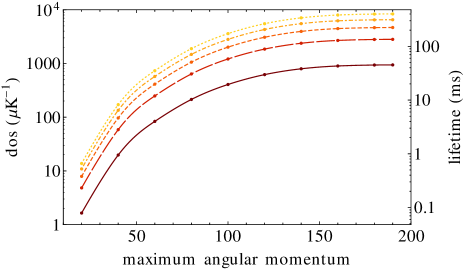
Figure 1: (Color online) Ro-vibrational density of states of RbCs + RbCs collisions as a function of the maximally allowed end-over-end angular momentum $L_{c}$ of the collision complex, for a total angular momentum $J=0-4,M=0$ (solid, long-dashed, dashed, dashed-dotted, and dotted line, respectively). The scale on the right axis gives the corresponding RRKM lifetime of the collision complex according to $\tau_{0}=2\pi\hbar\rho$.

An exemplary elastic cross section for RbCs molecular collisions in the absolute ground state ($v=n=0$, $M_{\mathrm{Cs}}=7/2$, $M_{\mathrm{Rb}}=3/2$ for both molecules) is presented in Fig. 2. Shown are cross sections for $s$-wave [yellow (light gray)] and $d$-wave [orange (gray)] scattering. This figure covers an energy range of twice the van der Waals energy $E_{\mathrm{vdW}}=\hbar^{3}(2m_{r})^{-3/2}C_{6}^{-1/2}$] and contains 10,000 energy points, evenly spaced on a logarithmic grid. At this resolution, most of the $s$-wave resonances are resolved, and the cross section frequently approaches the unitarity limit, $8\pi/k^{2}$. For $d$-wave scattering, these resonances are not resolved so well. It is clear from the figure that at typical ultracold temperatures $T=0.1-1$ K, these resonances can never be resolved.

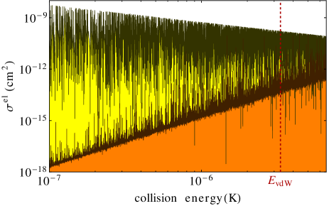
Figure 2: (Color online) Elastic $s$-wave [yellow (light gray)] and $d$-wave [orange (gray)] cross section of RbCs + RbCs. Incident channel is the absolute ground state ($v=n=0$, $M_{\mathrm{Cs}}=7/2$, $M_{\mathrm{Rb}}=3/2$ for both molecules).

IV Influence on scattering of non-reactive molecules

The extremely high density of states estimated in the previous section implies a striking feature of molecule-molecule cold collisions. Namely, molecules that meet on resonance may become lost in the complex for times on the order of many milliseconds, comparable to the time scales of a typical experiment. In this section we formulate a set of rate equations accounting for this occurrence, using RbCs as an example. The rate equations describe three separate events: i) a pair of RbCs molecules meet and stick together, thus temporarily transforming into four-body complexes, with number density $n_{c}$; ii) The complexes decay back into molecules on a time scale set by the mean lifetime of the resonant states; and iii) during the lifetime of the complex, another RbCs molecule can collide with it, leading almost certainly to trap loss. We deal with each of the three parts of this process in the following.

IV.1 Molecule-sticking rate

For RbCs in its absolute ground state, the number of open channels is exactly $N_{o}=1$. This circumstance automatically places resonant scattering in the limit where, on average, resonance widths are smaller than the mean resonance spacing, and resonances do not overlap. Thus only some fraction of the collision events lead to long-lived resonances, albeit very long-lived ones. We model the sticking process by ascribing to it a cross section which is zero away from resonance, but which contains resonances at the appropriate DOS and width distribution. Such a cross section is in fact afforded by the elastic cross section $\sigma^{\rm el}(E)$, which is easily computed from our statistical MQDT formalism.

The rate at which the complex-forming collisions happen is given by a thermally averaged rate constant, here distinguished by the partial wave $L,M_{L}$ considered:

$$K_{\rm mm}^{(L,M_{L})}(T)=\int_{0}^{\infty}\sigma_{L,M_{L}}^{\mathrm{el}}(E)\,vf(v)dv,$$ (8)

where “mm” stands for “molecule-molecule,” and

$$f(v)=\sqrt{\frac{2}{\pi}}\left(\frac{k_{b}T}{m_{r}}\right)^{-\frac{3}{2}}v^{2}e^{-m_{r}v^{2}/2k_{b}T}$$ (9)

is the Maxwell-Boltzmann distribution for the relative velocity for a given temperature $T$ of the initial molecular sample.

When the mean resonance spacing is far less than the temperature, as we assume, then these many resonances are averaged over. We can therefore replace the strongly-varying cross section by its mean value, taken over each of the isolated resonances separately, and averaged over the mean spacing $d=\rho^{-1}$ between resonances:

$$\bar{\sigma}_{L,M_{L}}^{\mathrm{el}}(E)=\frac{1}{d}\int_{E-d/2}^{E+d/2}\sigma_{L,M_{L}}^{\mathrm{el}}(\varepsilon)d\varepsilon.$$ (10)

This amounts to saying that only a fraction of collision energies, approximately $\Gamma(k)/d$, are on resonance and can lead to large sticking times, where $\Gamma(k)$ is the mean resonance width in the vicinity of energy $E=\hbar^{2}k^{2}/2m_{r}$. Note that the resonant cross sections scale as the unitarity limit, $\propto 1/k^{2}$, whereas resonance widths $\Gamma(k)\propto k^{2L+1}$, leading to a threshold law $K_{\rm mm}^{L,M_{L}}\propto k^{2L}$ for the sticking rate.

More quantitatively, we make use of the simple algebraic structure of the MQDT formalism, in the ultracold limit and for a single channel ($N_{a}=N_{o}=1$) the elastic cross section reads

$$\sigma_{L,M_{L}}^{\mathrm{el}}(E)=\Delta\frac{4\pi}{2m_{r}E}\frac{A(E,L)^{2}}{[K^{\mathrm{sr}}(E)]^{-2}+A(E,L)^{2}},$$ (11)

where $K^{\mathrm{sr}}=-\pi\sum_{\mu}W_{\mu}^{2}/(E-E_{\mu})$. In the ultracold limit, the energy dependent MQDT parameter $A(E,L)$ can be written down explicitly Ruzic et al. ,

$$A(E,L)^{1/2}=-\frac{\pi 2^{-2L-3/2}}{\Gamma(\frac{L}{2}+\frac{5}{4})\Gamma(L+\frac{1}{2})}R_{\mathrm{vdW}}^{L+\frac{1}{2}}\left(\frac{\hbar}{\sqrt{2m_{r}E}}\right)^{L+\frac{1}{2}}.$$ (12)

$R_{\mathrm{vdW}}=(2m_{r}C_{6}/\hbar^{2})^{1/4}$ is the van der Waals length scale. In deriving Eq. (11) we employed the ultracold limits $\mathcal{G}\rightarrow 0$ and $\eta\rightarrow 0$ of the remaining MQDT parameters Ruzic et al. . In the vicinity of a resonance at $E_{0}$ and replacing the short- to long-range couplings $W_{\mu}$ by their average, $\pi W_{\mu}^{2}=\bar{\Gamma}/2$ Mayle et al. (2012), Eq. (11) becomes

$$\sigma_{L,M_{L}}^{\mathrm{el}}(E)\approx\Delta\frac{4\pi}{2m_{r}E}\frac{[A(E,L)\bar{\Gamma}/2]^{2}}{(E-E_{0})^{2}+[A(E,L)\bar{\Gamma}/2]^{2}}.$$ (13)

Assuming additionally that $A(E,L)$ is approximately constant within the range of a single resonance, Eqs. (10,13) yield the mean cross section at collision energy $E$,

$$\bar{\sigma}_{L,M_{L}}^{\mathrm{el}}(E)=\Delta\frac{4\pi}{2m_{r}E}A(E,L).$$ (14)

We therefore identify the rate constant for collisional sticking as

$$\bar{K}_{\rm mm}^{(L,M_{L})}(T) =\int_{0}^{\infty}\bar{\sigma}_{L,M_{L}}^{\mathrm{el}}\!(E)\,vf(v)dv$$ (15)

$$=\Delta\frac{2^{-3L+2}\pi^{5/2}R_{\mathrm{vdW}}^{2L+1}}{\Gamma(\frac{L}{2}+\frac{1}{4})^{2}\Gamma(L+\frac{3}{2})}\frac{m_{r}^{L-1}}{\hbar^{2L-1}}(k_{B}T)^{L}.$$ (16)

Interestingly, this expression agrees exactly with the inelastic rate constant derived for scattering in the presence of rapid loss due to chemical reactions Quéméner et al. (2011), modeled by assuming unit loss probability at each collision energy. The effect of averaging over a very large number of very narrow resonances has produced a cross section that is equivalent to full absorption at every collision energy, modified by the appropriate threshold laws. This is a tremendous simplification: rather than even attempt to deal explicitly with real potential energy surfaces and the many resonances they engender, we are able to cut immediately to the observable consequence, namely, temperature-dependent sticking probabilities.

Armed with this insight, we can immediately extend the model to nonzero electric fields, assuming that the field significantly affects only long-range physics, and molecules reaching small $R$ vanish with unit probability. This problem can be solved exactly as in Refs. Quéméner and Bohn (2010a); Quéméner et al. (2011). The resulting rate constants for our example of RbCs collisions are reproduced in Fig. 3. References Quéméner and Bohn (2010a); Quéméner et al. (2011) predict that rate constants for loss in partial wave $L$ scales as $d^{4L+2}$ for induced dipole moment $d$. Hence, for small dipole moments $s$-wave scattering prevails. In Fig. 3 the rate constant in the upper curve shows an initial rise $\propto d^{2}$ for $s$-waves, until it saturates at around $d\sim 0.25$D Idziaszek et al. (2010). There is then a second rise, owing to the rapid increase of loss rate in the $d$-wave channel, which dominates the loss beyond $d\sim 0.6$D. For scattering with orbital angular momentum component $M_{L}=2$ (lower curve), the $d$-wave rise is still apparent, but there is, of course, no $s$-wave contribution at smaller dipole moment.

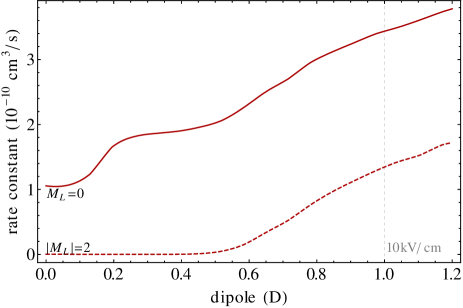
Figure 3: Quenching rate constants of two indistinguishable bosonic polar ⁸⁷Rb¹³³Cs molecules as a function of the induced dipole moment for a temperature of $T=1\,\mu$K. The solid line represents the $M_{L}=0$ contribution, the dashed line the $M_{L}=2$ (equal to the $M_{L}=-2$) contribution.

IV.2 Mean lifetime of the complex

The resonant complexes formed in molecule-molecule collisions will eventually decay back into pairs of molecules. The lifetime of the complex at a given collision energy can be quantified by means of the time delay Wigner (1955); Smith (1960); Fano and Rau (1986),

$$\tau_{\mathrm{delay}}=2\hbar\frac{d\delta}{dE}.$$ (17)

Here $\delta$ is the eigenphase sum, that is, the sum of the inverse tangents of the eigenvalues of the $K$-matrix. Employing the same approximations as in deriving Eqs. (13,14), the time delay close to a resonance at $E_{0}$ reads

$$\tau_{\mathrm{delay}}\approx 2\hbar\frac{A(E,L)\bar{\Gamma}/2}{(E-E_{0})^{2}+[A(E,L)\bar{\Gamma}/2]^{2}},$$ (18)

and therefore the mean time delay becomes

$$\bar{\tau}_{\mathrm{delay}}=\rho\int_{E_{0}-1/(2\rho)}^{E_{0}+1/(2\rho)}2\hbar\frac{d\delta}{dE}dE=2\pi\hbar\rho.$$ (19)

This is just the lifetime of the resonant complex as predicted by the RRKM theory, Eq. (6). Just as we need not consider individual resonances in the high-density limit, neither do we need to consider their individual lifetimes – another simplification. We therefore define, for each partial wave $L$, a decay rate of the complexes, $\gamma_{L}=\bar{\tau}_{\mathrm{delay}}^{-1}$, which follows immediately from the DOS in Table 1.

IV.3 Rate equations

We are now in a position to formulate the rate equations for the ultracold gas of RbCs molecules. Denote by $n_{m}$ the number density of these molecules and by $n_{c,L}$ the number density of the transient four-body complexes formed from initial partial wave $L$ of the molecule-molecule scattering. Because the molecule-molecule scattering rates $K_{\rm mm}^{(L,M_{L})}$ and the decay rates are different for different $L$, we explicitly add together the different contributions, as if they were independent. We assume that molecule-complex collisions are $s$-wave dominated and field independent, and hence described by a universal rate of the form Eq. (16), with $L=0$ and appropriate values for the reduced mass and $C_{6}$. Rate equations that describe the sticking of two molecules to form the complex, the subsequent decay of the complex, and demolition of a complex due to collision with another molecule, are given by

$$\dot{n}_{m} =\sum_{L}\left(-n_{m}^{2}\sum_{M_{L}}K_{\rm mm}^{(L,M_{L})}+2\gamma_{L}n_{c,L}-K_{\rm mc}n_{m}n_{c,L}\right),$$ (20)

$$\dot{n}_{c,L} =\tfrac{1}{2}n_{m}^{2}\sum_{M_{L}}K_{\rm mm}^{(L,M_{L})}-\gamma_{L}n_{c,L}-K_{\rm mc}n_{m}n_{c,L}.$$ (21)

Here $K_{\rm mm}^{(L,M_{L})}$ and $K_{\rm mc}$ are the molecule-molecule and molecule-complex collision rate constants. As shown in Table 1, different total angular momenta $J$ lead to different densities of states and therefore different lifetimes of the collision complex (recall that $J$ is identical with the incident partial wave $L$ of the collision). This is accounted for in Eq. (20) by allowing the formation of different, independent collision complexes with densities $n_{c,L}$, each possessing its own decay rate $\gamma_{L}$. The complexes are populated according to the molecular collision rate $K_{\rm mm}^{(L,M_{L})}$ for the given partial wave $L$ as extracted from Fig. 3. The molecule-complex collision rate constants are considered equal for all complexes. Moreover, we assume that different $M_{L}$ give rise to the same DOS and therefore to the same lifetime $\gamma_{L}$.

The time-dependent molecular density $n_{m}(t)$ resulting from a numerical integration of Eqs. (20,21), starting from an initial molecular density $n_{0}$, is presented in Fig. 4(a). Results are shown for two different electric field strengths (0 and 10 kV/cm, respectively). Initially, when $n_{c}(t)\ll n_{m}(t)$, Eq. (20) is dominated by the loss due to complex formation at a rate $-K_{\rm mm}n_{0}^{2}$, where $K_{\rm mm}=\sum_{L,M_{L}}K_{\rm mm}^{(L,M_{L})}$ is the total molecular loss rate. After some time $t^{\prime}$ this initial, fast decay turns over into a slow decay due to lossy molecule-complex collisions. Some insights can be gained by setting $K_{\rm mc}=0$ for the moment, that is, no lossy molecule-complex collisions. The resulting molecular density $n_{m}^{(0)}(t)$ is shown in Fig. 4(a) as dotted (assuming only $s$-wave collisions) and dashed ($d$-wave collisions) lines. In this case, the solution $n_{m}^{(0)}(t)$ reaches an equilibrium,

$$n_{m}^{(0)}(t) \rightarrow\frac{\sqrt{1+4n_{0}K_{\rm mm}\gamma^{-1}}-1}{2K_{\rm mm}\gamma^{-1}},$$ (22)

$$\frac{n_{m}^{(0)}(t)^{2}}{n_{c}^{(0)}(t)} \rightarrow\frac{2\gamma}{K_{\rm mm}},$$ (23)

as $t\gg t^{\prime}$. The timescale $t^{\prime}$, on which the initial linear decay turns to reach this dynamical equilibrium, can be extracted from the analytic solution $n_{m}^{(0)}(t)$ as

$$t^{\prime}=\frac{2}{\sqrt{\gamma^{2}+K_{\rm mm}\gamma n_{0}}}.$$ (24)

This time is indicated in Fig. 4(a) by arrows, assuming purely $s$-wave collisions for zero field and $d$-wave collisions for 10 kV/cm. Moreover, by inserting Eq. (23) into Eq. (20) one finds an expression for the slow final decay,

$$n_{m}(t)\approx\left[1+\alpha K_{\rm mm}K_{\rm mc}\gamma^{-1}n_{1}^{2}(t-t_{1})\right]^{-1/2},$$ (25)

where $n_{m}(t_{1})=n_{1}$ for some time $t_{1}>t^{\prime}$ at which the long-times behavior has already been reached. $\alpha$ acts as an empirical correction factor that accounts for Eq. (23) not reaching the dynamical equilibrium quite yet.

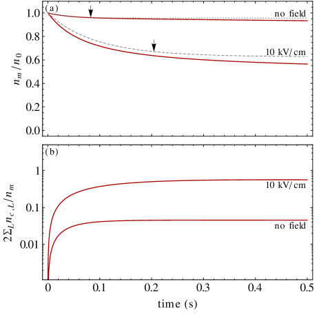
Figure 4: (a) Time evolution of the RbCs molecular density $n_{m}(t)$ for zero field (upper curves) and an applied electric field of 10 kV/cm (lower curves); $s$- and $d$-wave wave collisions are considered. Dotted ($s$-wave) and dashed ($d$-wave) lines are computed without particle loss due to complex-molecule collisions, that is, $K_{\rm mc}=0$ in Eqs. (20,21). The initial molecular density is $n_{0}=10^{10}\mathrm{cm}^{-3}$ at a assumed sample temperature of 1 $\mu$K. The arrows indicate the timescale $t^{\prime}$ as given by Eq. (24). (b) Evolution of the ratio of molecules bound in complexes to free molecules. The same set of parameters as in panel (a) is used.

The time evolution of the molecular density is vastly influenced by external electric fields, scaling as $d^{4L+2}$ for dipole moment $d$ and partial wave $L$ Quéméner et al. (2011). As a result, for our example in Fig. 4(a), the molecular density after its initial, fast decay is almost cut in half for fields $\gtrsim 10$ kV/cm. Even the field-free case is not free of losses due to complex formation; however, over 90% of the initial density is retained. Hence, in spite of not being chemically reactive, ultracold RbCs may still manifest substantial loss, which will become faster in an electric field.

This is emphasized by Fig. 4(b), where we show the ratio of total molecules bound in complexes to free molecules, for the same set of field strengths as in panel (a). As expected from Fig. 4(a), for zero electric field only a very small fraction of the molecules is bound in complexes. This changes drastically, however, once the field is turned on. For 10 kV/cm, half the molecules are trapped inside collision complexes at any given time.

The apparent loss of molecules depends on the magnitude of any applied electric field, but also on the initial density $n_{0}$ of molecules, cf. Eq. (22). In Fig. 5 we show the results for $n_{0}=10^{11}\mathrm{cm}^{-3}$, that is, increased by one order of magnitude compared to Fig. 4. Now, even zero electric field leads to significant molecule loss. For 10 kV/cm, after only half a second fewer than 20% of the initial molecular density is retained.

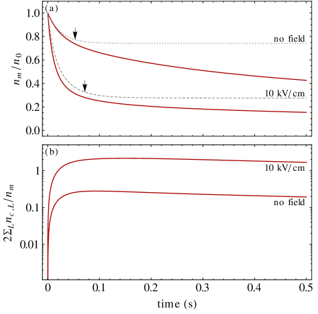
Figure 5: Same as in Fig. 4 but for a higher initial density of $n_{0}=10^{11}\mathrm{cm}^{-3}$.

Experimental data on loss as in Figs. (4,5) can strongly constrain the parameters of the model At short times, the initial decay is given by $-K_{\rm mm}n_{0}$. With the initial density $n_{0}$ usually well known, one can therefore extract $K_{\rm mm}$ straightforwardly. At intermediate times, $n_{m}(t)$ turns from its initial drop to its long-time behavior. This timescale, Eq. (24), is proportional to the lifetime of the complex. Hence, from experimental data, one could infer at least an estimate of the complex’ lifetime. Finally, at long times the decay of the molecular density is well fitted by Eq. (25), from which in turn the molecule-complex collision rate constant $K_{\rm mc}$ can be extracted.

V Influence on scattering of reactive molecules

The situation is completely different for a species that is chemically reactive at zero temperature, such as KRb. In this case, transition state theory dictates that the number of open channels $N_{o}$ includes also the product channels. These appear to be shockingly numerous, considering that the exoergicity of ground state KRb collisions is only 10.4 $\text{cm}^{-1}$ Meyer and Bohn (2010). Even within this small energy release, it is possible, in principle, to produce K₂ molecules with rotation quantum number up to $n_{K_{2}}=13$, or Rb₂ molecules up to $n_{Rb_{2}}=20$, or any energetically allowed combination. Moreover, the products can have any reasonable partial wave angular momentum $L_{K_{2}Rb_{2}}$ of the products about each other, provided that the total angular momentum ${\bf J}={\bf n}_{K_{2}}+{\bf n}_{Rb_{2}}+{\bf L}_{K_{2}Rb_{2}}$ is conserved.

Again assuming ergodicity in all degrees of freedom, we obtain $N_{o}$ by simply counting all possible exit channels consistent with conservation of angular momentum and energy, constructing molecular levels from the potentials in Falke et al. (2008); Strauss et al. (2010); Pashov et al. (2007). The result is a vast number of possible channels, which grows rapidly as a function of total angular momentum $J$. Accounting for all these possibilities, the resulting number of possible product channels are listed in Table 2 for various total $J$ but fixed $M=0$. No enhancement due to nuclear spins is considered here.

Also shown in the table is the corresponding RRKM decay rate into product channels. This width far exceeds the mean level spacing (by a factor of $N_{o}$, in fact), and renders the individual resonances unobservable. In fact, in this limit one expects collision cross sections to exhibit Ericson fluctuations, on a scale comparable to $\Gamma$ itself. Inasmuch this width is already of order $\mu$K (or $\sim 10$ Gauss in magnetic field), it is unlikely that any structure will be seen at all. Again, we are back to the simpler situation of studying non-resonant cross sections.

Indeed, the occurrence of many exit channels implies that the decay rate of the complex is extremely rapid, so rapid that the states of the complex are not significantly populated at all. An alternative way to view this circumstance is to note that in the statistical theory the probability of chemical reaction is $N_{o}/(N_{o}+1)\approx 1$, whereas the probability of elastic scattering back to the single initial channel is $1/(N_{0}+1)\ll 1$. Thus the scattering leads to unit probability of chemical reaction, as posited in Refs. Quéméner et al. (2011); Ospelkaus et al. (2010); Ni et al. (2010); Idziaszek et al. (2010); Idziaszek and Julienne (2010); Quéméner and Bohn (2010a); de Miranda et al. (2011). In fact, Ref. Idziaszek and Julienne (2010) provides a universal analytic expression of the inelastic rate constant for $p$-wave scattering with unit reaction loss probability, for identical fermionic molecules,

$$K^{\mathrm{in,uni}}_{L=1}=12\pi\frac{\hbar}{m_{r}}a_{1}(k\bar{a})^{2}\Delta.$$ (26)

Here, $\bar{a}=2\pi R_{\mathrm{vdW}}/\Gamma(1/4)^{2}$ and $\bar{a}_{1}=\bar{a}\,\Gamma(1/4)^{6}/[12\pi\Gamma(3/4)]^{2}$ are length scales of $s$- and $p$-wave scattering from a pure $C_{6}$ potential.

Table 2: Number of KRb + KRb $\rightarrow$ K₂ + Rb₂ product channels along with the predicted RRKM width, $\Gamma_{\mathrm{RRKM}}=N_{o}/2\pi\rho$, of the resonances. In calculating the latter, we use the densities of states provided in Table 1.

$J$	number of channels	$\Gamma_{\mathrm{RRKM}}(\mu\mathrm{K})$	$\Gamma_{\mathrm{RRKM}}(\mathrm{G})$
0	45055	2.21	7.78
1	131239	2.15	7.27
2	213521	2.11	7.42
3	291901	2.06	6.97

In Fig. 6 we compare representative inelastic $p$-wave scattering cross sections to the unit loss prediction Eq. (26). Rather than immediately employ the full number of open channels $N_{o}$ for this case (which is technically challenging even within our simplified model), we emphasize the trend for ever-larger $N_{o}$. Thus the solid black line shows an exemplary cross section for only $N_{o}=100$ open channels. In this case Ericson fluctuations occur on a sub-$\mu$K scale and are seen in the spectrum. However, even increasing the number of open channels to $N_{0}=1000$ (red line) almost completely washes out these fluctuations. Moreover, this result shows almost perfect agreement with the simple model in Eqn. (26). We find similar good agreement for different realizations of the statistical spectrum.

We conclude from this result that the realistic $N_{o}$, which is much larger still, will certainly lead to a featureless loss spectrum given by Eqn. (26). Thus the statistical model as deployed here vindicates the models in Refs. Quéméner et al. (2011); Ospelkaus et al. (2010); Ni et al. (2010); Idziaszek et al. (2010); Idziaszek and Julienne (2010); Quéméner and Bohn (2010a); de Miranda et al. (2011).

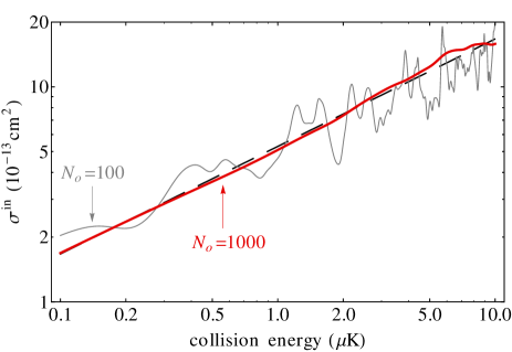
Figure 6: (Color online) Inelastic $p$-wave scattering cross section mimicking ultracold KRb collisions with $N_{o}=100$ (light gray) and $N_{o}=1000$ [red (dark gray)] product channels. The dashed line represents the analytic prediction for unit loss probability, cf. Eq. (26).

VI Summary

For collisions of alkali-metal dimer molecules, we have found that the density of ro-vibrational states is enormous, far too large to probe individual resonances even at the sub-$\mu$Kelvin energy resolution afforded by ultracold temperatures. Because of this circumstance, resonant collision rates are always averaged over many resonances, and the theoretical description of scattering is greatly simplified. Thus broad general conclusions can be drawn. For the case of chemically reactive molecules, the formation of a resonant state ensures that the atoms have ample opportunity to find their way into the product channels, at least for reactions that are assumed to be barrierless. This in turn leads to essentially unit probability of reaction in each collision event, consistent with interpretations of recent experiments in ultracold KRb gases.

Strikingly, even molecules that are not chemically reactive at zero temperature, in the presence of this vast number of resonances, behave as if they were chemically reactive, at least transiently. These molecules are capable of sticking together for a finite lifetime, which is dependent on the density of states. The longer this lifetime is, the more likely that the molecules bound in resonant complexes will be struck by other molecules and lost. Contrary to expectation, it may therefore be necessary to shield even non-reactive molecules from collisions by confining them to 1D lattices and immersing them in electric fields Büchler et al. (2007); Micheli et al. (2010); Quéméner and Bohn (2010b); de Miranda et al. (2011); Quéméner and Bohn (2011); Julienne et al. (2011).

A main quantitative uncertainty in the results described here is whether the full density of ro-vibrational states is actually populated in a collision, which may not be the case Nesbitt (2012). If it is not, then the time during which the molecules are stuck together reduces, and the loss rates may not be as great. Thus measurements of loss may provide direct insight into the four-body dynamics of the molecule-molecule complex.