Diffusivity of a random walk on random walks

Abstract

We consider a random walk $\left(Z^{(1)}_{n},\cdots,Z^{(K+1)}_{n}\right)\in\mathbb{Z}^{K+1}$ with the constraint that each coordinate of the walk is at distance one from the following one. In this paper, we show that this random walk is slowed down by a variance factor $\sigma_{K}^{2}=\frac{2}{K+2}$ with respect to the case of the classical simple random walk without constraint.

Keywords: Random walk, Graph, Central limit theorem

AMS classification (2000): 05C81, 60F05.

1 Presentation of the random walk

Let $\left(Z^{(1)}_{n},\cdots,Z^{(K+1)}_{n}\right)\in\mathbb{Z}^{K+1}$ denote the heights of $K+1$ simple random walks on $\mathbb{Z}$, conditioned on satisfying

$$\forall n\in\mathbb{N},\forall i\in\left[1,K\right],\left|Z^{(i+1)}_{n}-Z^{(i)}_{n}\right|=1.$$ (1)

More precisely, the random walk is a Markov chain on the state space of $K$-step walks in $\mathbb{Z}$

$$\mathcal{S}_{K}=\{(z^{(1)},\ldots,z^{(K+1)})\in\mathbb{Z}^{K+1},\quad\forall i\in\left[1,K\right],|z^{(i+1)}-z^{(i)}|=1\}$$

where the next step from $z\in\mathcal{S}_{K}$ is selected uniformly among the neighbours of $z$ in the usual lattice $\mathbb{Z}^{K+1}$ that belong to $\mathcal{S}_{K}$. In other words, we consider $K+1$ simple random walks on the lattice $\mathbb{Z}$ coupled under a shape condition.

As in the case of a simple random walk, the rescaled trajectory of a walker, say $Z^{(1)}$, will converge in law to a Brownian motion. However, it is interesting to note that the constraint between each coordinate only slow down the walk by decreasing its variance.

Since it is classical to illustrate for our students the simple random walk as the motion of a drunk man, we can illustrate the previous mathematical fact by considering the random walk as the motion of a chain of prisoners. It should convince even non mathematicians that the motion of the walk is slowed by the constraint. However it seems very hard to guess the variance from this comparison !

More precisely, denote

$$\forall t\geq 0,\forall n\in\mathbb{N},\xi_{t}^{(n)}=\frac{Z^{(1)}_{\lfloor nt\rfloor}}{\sqrt{n}},$$

where $\lfloor x\rfloor$ is the integer part of the real number $x.$

THEOREM 1.

The rescaled random walk $\left(\xi_{t}^{(n)}\right)_{t\geq 0}$ converges in law, as $n$ goes to infinity, to a Brownian motion with variance

$$\sigma_{K}^{2}=\frac{2}{K+2}.$$

Convergence to the Brownian motion is the usual invariance principle : the noteworthy statement here is that it is possible to give an explicit expression for the limit diffusivity of the process, and that its expression is particularly simple.

Our object of interest, the motion of $Z^{(1)},$ is a non-Markovian process that falls into the class of random walks with internal structure. Related questions of limit diffusivity for random walks conditioned to respect some geometric shape have been studied in the literature, under the name of “spider random walks” or “molecular spiders”, see [5]. The computation of the limit diffusion coefficient is also a central aim there, although the model and methods are different.

Our initial motivation was however more remote. Actually we first addressed this question starting from combinatorial problems related to $6$-Vertex model in relation with the Razumov Stroganov conjecture (See [2] for instance). The problem can also be related to random graph-homomorphisms (See [1]) or the Square Ice Model (See [3] where $Z^{(1)}$ evolves on a torus.)

Roughly speaking we can say that, in the literature we read, the authors consider questions related to the uniform distribution on a sequence of finite graphs $G_{K}$ and wonder about various asymptotics when $K\to+\infty.$ Later in the article the evolution of $Z_{n}$ will be described as the simple random walk on a graph $G_{K}.$ Hence on the one hand our problem is a very simplified version of the problems stated above, On the other hand we were surprised to have such a simple formula for $\sigma_{K}^{2}=\frac{2}{K+2},$ which is true for all $K$ and not only for $K\to+\infty.$ We thought in the beginning that the proof of this fact should be simple but it turns out that, although elementary, the tools used to obtain the result are more sophisticated than expected. It is the aim of this note to show these tools.

To prove the theorem, we will look for a decomposition

$$Z^{(1)}_{n}=M_{n}+f(Z_{n-1},Z_{n}),$$

where $(M_{n})_{n\in\mathbb{N}}$ is a martingale, and where $f:\mathbb{Z}^{K+1}\times\mathbb{Z}^{K+1}\rightarrow\mathbb{R}$ is a bounded function. We will then show that the following limit exists :

$$\sigma_{K}^{2}=\lim_{n\rightarrow\infty}\frac{1}{n}\mathbb{E}\left[M_{n}^{2}\right].$$

and that it is indeed the desired diffusivity. The path to this conclusion is akin to classical results for Central Limit Theorems for Markov chains (E.g. [4]).

We will use another equivalent, albeit more geometric, point of view on this decomposition. We split the chain in two parts : on the one hand, the motion of one of the walkers, and on the other hand, the relative positions of the walkers (which we call the “shape” of the chain at a given time). The latter part is a Markov chain over the state space $\{-1,1\}^{K}$ and our quantity of interest is (almost) an observable of this chain. Computing the martingale decomposition that we wish for amounts to decomposing a discrete vector field over this new state space into a divergence-free part (corresponding to the martingale part) and a gradient part (corresponding to the function $f$). Owing to a particular geometric property of this vector field, for which we coin the term “stationarity”, it is indeed possible to perform this calculation explicitly.

2 The random walk with constraint

Let us denote

$$\forall n\in\mathbb{N},\forall i\in\left[1,K\right],Y_{n}^{(i)}=Z_{n}^{(i+1)}-Z_{n}^{(i)},$$

and

$$Y_{n}=\left(Y_{n}^{(1)},\cdots,Y_{n}^{(K)}\right)\in\left\{-1,1\right\}^{K}.$$

Here $Y_{n}$ describes the shape of $\left(Z^{(1)}_{n},\cdots,Z^{(K+1)}_{n}\right)\in\mathbb{Z}^{K+1}$, i.e. the position of each $Z_{n}^{(i)}$ relatively to the previous one, and belongs to $V_{K}=\left\{-1,1\right\}^{K}$, whereas $Z^{(1)}_{n}$ can be seen as the height of the first walker. Obviously, the evolution of the chain of walkers may be described by the variables $\left(Z^{(1)}_{n},Y_{n}\right)_{n\in\mathbb{N}}$.

For a convenient analysis, we will represent our process as the simple random walk on a (multi)-graph $G_{K}$, which we define below.

Set $V_{K}=\{-1,1\}^{K}$ : the multi-graph $G_{K}$ is given as a triplet $(V_{K},E_{K}^{+},E_{K}^{-})$ where $E_{K}^{+},E_{K}^{-}\subset V_{K}\times V_{K}$ are two edge sets, called respectively the set of “positive“ and ”negative“ edges. A couple $(a,b)\in V_{K}\times V_{K}$, $a\neq b$, belongs to $E_{K}^{+}$ if the vector $b-a\in\{-2,0,2\}^{K}$ has nonzero entries of alternating signs, with the first one negative. Moreover, $E_{K}^{+}$ also contains a loop from each $a\in V_{K}$ to itself, noted $(a,a)^{+}$.

Likewise, $E_{K}^{-}$ contains those couples $(a,b)\in V_{K}\times V_{K}$, $a\neq b$, such that $b-a\in\{-2,0,2\}^{K}$ has nonzero entries of alternating sign, with the first one positive, and self-loops noted $(a,a)^{-}$ for each $a\in V_{K}$.

Set $E_{K}=E_{K}^{+}\cup E_{K}^{-}$. Finally, we consider the following function on $E_{K}.$

DEFINITION 1.

Let $A:E_{K}\rightarrow\{1,-1\}$ be the function that takes the value $1$ on $E_{K}^{+}$ and $-1$ on $E_{K}^{-}$. Note that we have, for any $a\in V_{K}$, $A((a,a)^{\pm})=\pm 1$.

PROPOSITION 1.

Let $(W^{K}_{n})_{n\geq 0}$ be the simple random walk on $G_{K}$. The processes $\left(Y_{n},Z^{(1)}_{n}\right)_{n\in\mathbb{N}}$ and $\Big{(}W^{K}_{n},\sum_{j=1}^{n}A(W^{K}_{j-1},W^{K}_{j})\Big{)}_{n\in\mathbb{N}}$ have the same distribution.

Proof.

It is sufficient to prove that the two Markov chains (taking values in $\left\{-1,1\right\}^{K}\times\mathbb{Z}$) $\left(Y_{n},Z^{(1)}_{n}\right)_{n\in\mathbb{N}}$ and $\Big{(}W^{K}_{n},\sum_{j=1}^{n}A(W^{K}_{j-1},W^{K}_{j})\Big{)}_{n\in\mathbb{N}}$ have the same transition matrix.

We claim that

$$\mathcal{L}\left(Y_{n+1}-Y_{n},Z^{(1)}_{n+1}-Z^{(1)}_{n}|Y_{n},Z_{n}^{(1)}\right)=\\ \mathcal{L}\left(W_{n+1}-W_{n},A(W^{K}_{n},W^{K}_{n+1})|W_{n},\sum_{j=1}^{n}A(W^{K}_{j-1},W^{K}_{j})\right).$$

Recall that $\mathcal{S}_{K}=\left\{z\in\mathbb{Z}^{K+1},\forall i\in[1,K],\left|z^{(i+1)}-z^{(i)}\right|=1\right\}$. Denote

$$\mathcal{A}=\left\{(z_{1},z_{2})\in\mathcal{S}_{K}^{2},\forall i\in[1,K+1],\left|z_{1}^{(i)}-z_{2}^{(i)}\right|=1\right\}.$$

Since $(Z_{n})_{n\in\mathbb{N}}$ and $(W_{n})_{n\in\mathbb{N}}$ are both simple random walks, the corresponding transition matrices are given respectively by

$$P^{Z}_{z_{1},z_{2}} =\frac{1}{\mbox{Card}\left\{z\in\mathcal{S},(z_{1},z)\in\mathcal{A}\right\}}1\!\!1_{(z_{1},z_{2})\in\mathcal{A}}$$

$$P^{W}_{w_{1},w_{2}} =\frac{1}{\mbox{Card}\left\{w\in\left\{-1,1\right\}^{K},(w_{1},w)\in E_{K}\right\}}1\!\!1_{(w_{1},w_{2})\in E_{K}}.$$

Denote now

$$\delta:\; \mathcal{S}\rightarrow\{-1,1\}^{K}$$

$$(z^{(1)},\ldots,z^{(K+1)})\mapsto(z^{(2)}-z^{(1)},\ldots,z^{(K+1)}-z^{(K)}),$$

so that $Y_{n}=\delta(Z_{n}),n\in\mathbb{N}$.

To prove the proposition, it is sufficient to prove that

$$(z_{1},z_{2})\in\mathcal{A}\Leftrightarrow\left|z^{(1)}_{2}-z^{(1)}_{1}\right|=1\text{ and }\delta(z_{2})-\delta(z_{1})\in E_{K}^{\epsilon},$$

where $\epsilon=-\operatorname{sgn}(z^{(1)}_{2}-z^{(1)}_{1})$ (and $\operatorname{sgn}$ is the sign function).

First note that, if $\epsilon=\pm 1$, and if $\forall i\in[1,K+1],z_{1}^{(i)}=z_{2}^{(i)}-\epsilon$, then $(z_{1},z_{2})\in\mathcal{A}$. Moreover, we have in this case $\delta(z_{1})=\delta(z_{2})$, and $(\delta(z_{1}),\delta(z_{2}))\in E_{K}^{\epsilon}$ as claimed. On the other hand, if $\delta(z_{1})=\delta(z_{2})$ and $z_{2}^{(1)}-z^{(1)}_{1}=\epsilon\in\{-1,1\}$, then $\forall i\in[1,K+1],z_{1}^{(i)}=z_{2}^{(i)}+\epsilon$.

For the chain, it means that, if $Y_{n+1}=Y_{n}$ then $Z^{(1)}_{n+1}-Z^{(1)}_{n}$ is $+1,-1$ with equal probability $\frac{1}{2}$ independently of $Y_{n},Y_{n+1},Z^{(1)}_{n}$.

Assume now that $z_{1}\neq z_{2}$. We will prove that $(\delta(z_{1}),\delta(z_{1}))\in E_{K}^{\epsilon}$, where $\epsilon=z^{(1)}_{1}-z^{(1)}_{2}$, i.e. $\delta(z_{2})-\delta(z_{1})\in\{-2,0,2\}^{K}$, with nonzero entries of alternating signs, and a first one of the sign of $\epsilon$.

Indeed, there is a first index

$$\tau_{1}=\inf\{i\in\left[1,K\right],\;\mbox{such that}\quad\delta(z_{1})^{(i)}\neq\delta(z_{2})^{(i)}\}.$$

There are two possible cases

$$\delta(z_{1})^{(\tau_{1})}=+1,\;\delta(z_{2})^{(\tau_{1})}=-1,\;z^{(\tau_{1})}_{2}=z^{(\tau_{1})}_{1}+1,\;z^{(\tau_{1}+1)}_{2}=z_{1}^{(\tau_{1}+1)}-1,$$

$$\delta(z_{1})^{(\tau_{1})}=-1,\;\delta(z_{2})^{(\tau_{1})}=+1,\;z^{(\tau_{1})}_{2}=z^{(\tau_{1})}_{1}-1,\;z^{(\tau_{1}+1)}_{2}=z^{(\tau_{1}+1)}_{1}+1.$$

In the two cases we have $A(\delta(z_{1}),\delta(z_{2}))=z_{2}^{(\tau_{1})}-z_{1}^{(\tau_{1})}=z_{2}^{(1)}-z_{1}^{(1)}.$

Furthermore, we have

$$\delta(z_{2})^{(\tau_{1})}-\delta(z_{1})^{(\tau_{1})}=-2A(\delta(z_{1}),\delta(z_{2})).$$

Then if $\tau_{1}<K$ let us define

$$\tau_{2}=\inf\{i\in\left[\tau_{1}+1,K\right],\;\mbox{such that}\quad\delta(z_{2})^{(i)}\neq\delta(z_{1})^{(i)}\},$$

where we set by convention $\tau_{2}=K+1,$ if the condition defining the infimum is never satisfied.

Using the same arguments, we get

$$\delta(z_{2})^{(\tau_{2})}-\delta(z_{1})^{(\tau_{2})}=2A(\delta(z_{1}),\delta(z_{2})).$$

By induction one can define

$$\tau_{j}=\inf\{i\in\left[\tau_{j-1}+1,K\right],\;\mbox{such that}\quad\delta(z_{1})^{(i)}\neq\delta(z_{2})^{(i)}\},$$

until $\tau_{j-1}\geq K.$

We have

$$\delta(z_{2})^{(\tau_{j})}-\delta(z_{1})^{(\tau_{j})}=2(-1)^{j}A(\delta(z_{1}),\delta(z_{2})).$$

By definition, we get $(\delta(z_{1}),\delta(z_{2}))\in E_{K}^{\epsilon},$ where $\epsilon=z_{1}^{(1)}-z_{2}^{(1)}$.

On the other hand, if $(\delta(z_{1}),\delta(z_{2}))\in E_{K}^{\epsilon}$, where $\epsilon=z^{(1)}_{1}-z^{(1)}_{2}\in\{-1,1\}$, then one can recover explicitly $(z_{1},z_{2})$ from the definition of $\delta$. Moreover, the condition $\forall i\in[1,K+1],\left|z_{2}^{(i)}-z_{1}^{(i)}\right|=1$ is implied by the previous arguments (following the definitions of the $\tau_{j}$).

∎

We may denote, $Y_{n}\overset{e}{\rightarrow}Y_{n+1}$ when $e\in E^{+}$ ($Z^{(1)}_{n+1}=Z^{(1)}_{n}+1$) and $Y_{n}\overset{e}{\leftarrow}Y_{n+1}$ when $e\in E^{-}$ ($Z^{(1)}_{n+1}=Z^{(1)}_{n}-1$).

For a general $a\in V_{K}$ the previous enumeration of its neighbors is surprisingly complicated but we can provide some simple examples.

For instance if $a=(1,\ldots,1)\in V_{K},$ has only $K+2$ neighbors:

$$a \leftarrow a$$

$$a \rightarrow a$$

$$\forall i\in[1,K],a \rightarrow(1,\cdots,-1,\cdots,1),$$ (2)

where the $-1$ is in the $i$-th position.

Note now that the graph $G_{K}$ can also be described inductively : there are only six following possibilities for $(Z^{(1)}_{n},Z^{(2)}_{n},Z^{(1)}_{n+1},Z^{(2)}_{n+1})$, described below:

In the figure, we have used the concatenation notation : given a string $a$, the string $1a$, resp. $(-1)a$, is obtained by adding a $1$, resp. $-1$ in front of $a$. Looking only at the $3$ cases such that $Z^{(1)}_{n+1}-Z^{(1)}_{n}=1$, we can deduce the construction of $G_{K+1}^{+}$ from $G_{K}^{+}$:

$$V_{K+1} =\left\{-1,1\right\}^{K+1}$$

$$E_{K+1}^{+} =\left\{(1a,1b),(a,b)\in E_{K}^{+}\right\}\cup\left\{((-1)a,(-1)b),(a,b)\in E_{K}^{+}\right\}\cup\left\{(1a,(-1)b),(a,b)\in E_{K}^{-}\right\}$$

Figure 1 shows the first two graphs $G_{1}^{+}$ and $G_{2}^{+}$. Note that each edge of $G_{1}$ gives $3$ edges for $G_{2}$, one on each facet $\left\{1a,a\in V_{K}\right\}$, and $\left\{(-1)a,a\in V_{K}\right\}$ and one crossing from the facet $\left\{1a,a\in V_{K}\right\}$ to the facet $\left\{(-1)a,a\in V_{K}\right\}$.

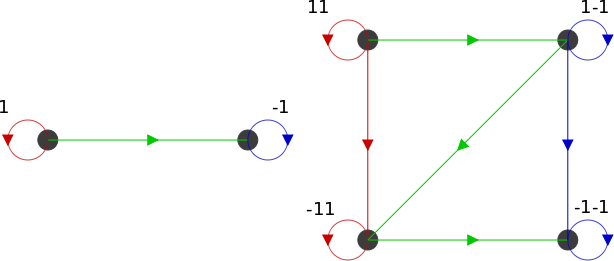
Figure 1: Construction of $G_{1}^{+}$ and $G_{2}^{+}$.

We obtain the cardinality $D_{K}$ of $E_{K}$ (as a multigraph) by induction:

$$D_{K}=2.3^{K}.$$

We will also make use of the number $\delta_{K}$ of edges of the form $(1a,(-1)b)\in E_{K}^{+}$ which can be computed by induction:

$$\delta_{K}=3^{K-1}.$$

Let us now describe vector fields on this graph.

3 Vector fields on graphs

In the previous section a function $A$ has been defined on edges of $G_{K}.$ We will consider here $A$ as a vector field on $G_{K}.$

3.1 Definitions

Let us first recall some classical definitions.

DEFINITION 2 (Vector fields).

A vector field on $G_{K}=\left(V_{K},E_{K}\right)$ is a function $S:E_{K}\rightarrow\mathbb{R}$ such that

$$\forall(a,b)\in E_{K},a\neq b,S(a,b)=-S(b,a).$$ (3)

and such that, for any $a\in V_{K}$, $S((a,a)^{+})=-S((a,a)^{-})$.

DEFINITION 3 (Gradient vector fields).

We say that the vector field $S$ on $G_{K}$ is a gradient vector field if there exists a function $f$ on the vertices of $G_{K}$ such that for each edge $(a,b)\in E_{K}$, $S(a,b)=f(b)-f(a)$. The gradient vector field associated with $f$ is denoted by $\nabla f$.

DEFINITION 4 (Divergence and divergence-free vector fields).

The divergence of a vector field $S$ at point $x\in G_{K}$ is defined by

$$(\nabla\cdot S)(x)=\sum_{(x,y)\in E_{K}}S(x,y).$$

We say that a vector field $S$ is divergence-free if its divergence vanishes at all points.

We can endow the set of vector fields with a scalar product

$$\langle S,S^{\prime}\rangle_{E_{K}}=\frac{1}{D_{K}}\sum_{e\in E_{K}}S(e)S^{\prime}(e).$$

Please note that the sum runs over all edges, including loops $(a,a)^{\pm}$.

Denote also, for any subsets $\phi,\psi$ of $V_{K}$,

$$J_{\phi,\psi}(S)=\sum_{a\in\phi,b\in\psi,(a,b)\in E_{K}}S(a,b),$$

the flux of $S$ going from $\phi$ to $\psi$. Note that a divergence free field $B$ verifies

$$\forall\phi\subset V_{K},J_{\phi,V_{K}\setminus\phi}(B)=0.$$

3.2 Hodge decomposition of vector fields on graphs

In analogy with the case of vector fields in Euclidean spaces, we can decompose any vector field on $G_{K}$ into the sum of a gradient vector field and a divergence-free field. The following proposition is well-known.

PROPOSITION 2.

Let $S$ be a vector field on $G_{K}$. There exist a unique gradient vector field $\nabla f$ and a unique divergence-free field $B$ such that

$$S=\nabla f+B.$$

Moreover $\langle\nabla f,B\rangle_{E_{K}}=0$

The last identity simply means that gradient fields and divergence-free fields are orthogonal complements of each other in the vector space of vector fields over $G_{K}$.

In our case we are interested in stationary vector fields.

DEFINITION 5 (Stationary vector field).

A subgraph $G$ of the complete graph on $\{-1,1\}^{K}$ is stationary, if the following holds. For $u,u^{\prime}\in\{-1,1\}^{K}$ and $v\in\mathbb{R}^{k}$ such that $u+v,u^{\prime}+v\in\{-1,1\}^{K},$ if $(u,u+v)$ is an edge of $G$, then $(u^{\prime},u^{\prime}+v)$ is an edge of $G$.

A vector field $S$ defined on a subgraph of the complete graph on $\{-1,1\}^{K}$ with a stationary domain is stationary if for all $(u,v)$ edges of $G$, $S(u,v)$ only depends on $u-v$ (where $\{-1,1\}^{K}$ is embedded in $\mathbb{R}^{K}$ in an obvious way).

REMARKS 1.

Note that, thanks to the construction of $E_{K}^{+}$, it is stationary. Moreover if $(u,u+v)\in E_{K}^{+}$ and $u^{\prime},u^{\prime}+v\in V_{K}$, then $(u^{\prime},u^{\prime}+v)\in E_{K}^{+}$ and thus the vector field $A$ taking values $1$, resp. $-1$, on $E_{K}^{+}$, resp. $E_{K}^{-}$, is stationary. So we may expect the gradient vector field $\nabla f$ in the Hodge decomposition of $A$ to be stationary. Unfortunately if $S$ is a stationary vector field on $G_{K}$ and its decomposition is

$$S=\nabla f+B$$

as per Proposition 2, then $\nabla f$ is not always stationary.

Nevertheless it turns out that the gradient vector field $\nabla f$ in the Hodge decomposition of $A$ is actually stationary as it will be shown in the next section.

3.3 Hodge decomposition of $A$

Let us recall the Definition 1 the vector field $A$ on $G_{K}$ is such that

$$\forall e\in E_{K}^{+},A(e)=1$$

$$\forall e\in E_{K}^{-},A(e)=-1.$$

In this section our aim is to compute a function $f$ such that

$$(\nabla\cdot A)(a)=(\nabla\cdot(\nabla f))(a)\quad\forall a\in V_{K}.$$ (4)

One can first remark that $\forall a\in V_{K}$

$$(\nabla\cdot A)(a)=\quad\mbox{Card}\{b\in V_{K},\;(a,b)\in E^{+}_{K}\}-\mbox{Card}\{b\in V_{K},\;(a,b)\in E^{-}_{K}\}.$$ (5)

In the previous equation we used the notation Card for cardinality of sets. We will introduce various notations related to other cardinalities

$$\alpha(a) = \mbox{Card}\{b\in V_{K},\;(a,b)\in E^{+}_{K}\}$$ (6)

$$\bar{\alpha}(a) = \mbox{Card}\{b\in V_{K},\;(a,b)\in E^{-}_{K}\}.$$ (7)

Then we need also to define for $0\leq k\leq K,$ $\alpha_{k}(a)$ the number of the vertices $b$ such that $(a,b)\in E^{+}_{K}$ with $k$ digits $i\in\{1,\ldots,K\}$ such that $a_{i}\neq b_{i}.$ Similarly $\bar{\alpha}_{k}(a)$ is the number of the vertices $b$ such that $(a,b)\in E^{-}_{K}$ and $k$ digits $i\in\{1,\ldots,K\}$ such that $a_{i}\neq b_{i}.$ Then we consider $\alpha_{ev}(a)=\sum_{k\;\;even}\alpha_{k}(a)$ and $\alpha_{od}(a)=\sum_{k\;\;odd}\alpha_{k}(a).$ Similarly $\bar{\alpha}_{ev}(a)=\sum_{k\;\;even}\bar{\alpha}_{k}(a)$ and $\bar{\alpha}_{od}(a)=\sum_{k\;\;odd}\bar{\alpha}_{k}(a).$

Let us consider the function $f_{1}$ on $V_{K}$ such that

$$f_{1}(a)=\alpha_{1}(a)-\bar{\alpha}_{1}(a)=\sum_{i=1}^{K}a_{i}.$$ (8)

The last equation is trivial since $\alpha_{1}(a)$ is the number of the $a_{i}$s equal to $1$ and $\bar{\alpha}_{1}(a)$ the number of $a_{i}$s equal to $-1.$ Obviously we also get

$$\alpha_{1}(a)+\bar{\alpha}_{1}(a)=K$$ (9)

for any vertex $a$ in $V_{K}.$ Let us remark that for any function $f$ on $V_{K}$

$$(\nabla\cdot(\nabla f))(a)=\sum_{(a,b)\in E_{K}}f(b)-f(a).$$

Since $f_{1}$ yields the sum of the digits of any vertex, we first observe that if $(a,b)\in E_{K}$ and the number of digits $i\in\{1,\ldots,K\}$ such that $a_{i}\neq b_{i}$ is even then $f_{1}(b)-f_{1}(a)=0.$ If the number of digits $i\in\{1,\ldots,K\}$ such that $a_{i}\neq b_{i}$ is odd and $(a,b)\in E_{K}^{+}$ then $f_{1}(b)-f_{1}(a)=-2.$ One can then deduce that

$$(\nabla\cdot(\nabla f_{1}))(a)=-2(\alpha_{od}(a)-\bar{\alpha}_{od}(a)).$$ (10)

It turns out that if we consider the function $f_{2}$ on $V_{K}$ such that

$$f_{2}(a)=\alpha_{2}(a)-\bar{\alpha}_{2}(a),$$ (11)

then

$$(\nabla\cdot(\nabla f_{2}))(a)=-(K+2)(\alpha_{ev}(a)-\bar{\alpha}_{ev}(a)).$$ (12)

We will prove (12) by induction on $K.$ To do that we split $(\nabla\cdot(\nabla f_{2}))$ into the sum of two functions

$$\phi(a) = \sum_{(a,b)\in E^{+}_{K}}f_{2}(b)-f_{2}(a)$$ (13)

$$\bar{\phi}(a) = \sum_{(a,b)\in E^{-}_{K}}f_{2}(b)-f_{2}(a).$$ (14)

To proceed the induction argument we remark that for any vertex $a$ in $V_{K}$

$$f_{1}(1a) = f_{1}(a)+1$$ (15)

$$f_{1}(-1a) = f_{1}(a)-1$$ (16)

$$f_{2}(1a) = f_{2}(a)+\bar{\alpha}_{1}(a)$$ (17)

$$f_{2}(-1a) = f_{2}(a)-\alpha_{1}(a).$$ (18)

We will then compute $\phi(1a),\;\phi(-1a),\;\bar{\phi}(1a),\;\bar{\phi}(-1a).$ The easiest computation is

$$\bar{\phi}(1a) = \sum_{(1a,b)\in E^{-}_{K+1}}f_{2}(b)-f_{2}(1a)$$

$$= \sum_{(a,c)\in E^{-}_{K}}f_{2}(1c)-f_{2}(1a),$$

since $(1a,-1c)\in E^{+}_{K+1}.$ Then

$$\bar{\phi}(1a) = \sum_{(a,c)\in E^{-}_{K}}f_{2}(c)-f_{2}(a)+\sum_{(a,c)\in E^{-}_{K}}\bar{\alpha}_{1}(c)-\bar{\alpha}_{1}(a).$$

To evaluate $\sum_{(a,c)\in E^{-}_{K}}\bar{\alpha}_{1}(c)-\bar{\alpha}_{1}(a)$ we use that $\bar{\alpha}_{1}(a)$ is the number of digits equal to $-1$ in $a.$ If $(a,c)\in E^{-}_{K}$ and if the number of $a_{i}\neq c_{i}$ is even then $\bar{\alpha}_{1}(c)=\bar{\alpha}_{1}(a).$ If this number is odd then $\bar{\alpha}_{1}(c)=\bar{\alpha}_{1}(a)-1.$ Therefore $\sum_{(a,c)\in E^{-}_{K}}\bar{\alpha}_{1}(c)-\bar{\alpha}_{1}(a)=-\bar{\alpha}_{od}(a).$ Hence

$$\bar{\phi}(1a) = \bar{\phi}(a)-\bar{\alpha}_{od}(a).$$ (19)

One also get in the same way

$$\phi(-1a)=\phi(a)-\alpha_{od}(a).$$ (20)

The induction is a bit more involved for

$$\phi(1a) = \sum_{(1a,b)\in E^{+}_{K+1}}f_{2}(b)-f_{2}(1a)$$

$$= \sum_{(1a,1c)\in E^{+}_{K+1}}f_{2}(1c)-f_{2}(1a)+\sum_{(1a,-1c)\in E^{+}_{K+1}}f_{2}(-1c)-f_{2}(1a).$$

Because of (17)

$$\sum_{(1a,1c)\in E^{+}_{K+1}}f_{2}(1c)-f_{2}(1a) = \sum_{(a,c)\in E^{+}_{K}}f_{2}(c)-f_{2}(a)+\sum_{(a,c)\in E^{+}_{K}}\bar{\alpha}_{1}(c)-\bar{\alpha}_{1}(a)$$

$$= \phi(a)+\alpha_{od}(a).$$

Then

$$\sum_{(1a,-1c)\in E^{+}_{K+1}}f_{2}(-1c)-f_{2}(1a) = \sum_{(a,c)\in E^{-}_{K}}f_{2}(c)-f_{2}(a)-\sum_{(a,c)\in E^{-}_{K}}\alpha_{1}(c)+\bar{\alpha}_{1}(a)$$

$$= \bar{\phi}(a)-\sum_{(a,c)\in E^{-}_{K}}\alpha_{1}(c)+\bar{\alpha}_{1}(c)$$

$$\phantom{\bar{\phi}(a)}+\sum_{(a,c)\in E^{+}_{K}}\bar{\alpha}_{1}(c)-\bar{\alpha}_{1}(a)$$

$$= \bar{\phi}(a)-K\bar{\alpha}(a)-\bar{\alpha}_{od}(a).$$

Hence

$$\phi(1a)=\phi(a)+\bar{\phi}(a)+\alpha_{od}(a)-\bar{\alpha}_{od}(a)-K\bar{\alpha}(a).$$ (21)

Similarly we get

$$\bar{\phi}(-1a)=\phi(a)+\bar{\phi}(a)-\alpha_{od}(a)+\bar{\alpha}_{od}(a)+K\bar{\alpha}(a).$$ (22)

We can now evaluate the functions $\phi,\;\bar{\phi}.$

LEMMA 1.

$\forall a\in V_{K},$

$$\phi(a)=\bar{\alpha}_{ev}(a)-(K+1)\alpha_{ev}(a)+\alpha_{od}(a)+\bar{\alpha}_{od}(a)$$ (23)

$$\bar{\phi}(a)=-\alpha_{ev}(a)+(K+1)\bar{\alpha}_{ev}(a)-\bar{\alpha}_{od}(a)-\alpha_{od}(a)$$ (24)

Proof.

We will only sketch the proof performed by an easy induction on $K$ for $\phi,$ computations are similar for $\bar{\phi}.$ Let us assume that (23), (24) hold for $K,$ we have to compute $\phi(1a)$ and $\phi(-1a)$ and check that they fulfill  (23), (24) for $K+1.$ Because of (21)

$$\phi(1a)=\phi(a)+\bar{\phi}(a)+\alpha_{od}(a)-\bar{\alpha}_{od}(a)-K\bar{\alpha}_{ev}(a)-K\bar{\alpha}_{od}(a).$$

One can check that $\bar{\alpha}_{ev}(1a)=\bar{\alpha}_{ev}(a),\;\alpha_{ev}(1a)=\alpha_{ev}(a)+\bar{\alpha}_{od}(a),\;\alpha_{od}(1a)=\alpha_{od}(a)+\bar{\alpha}_{ev}(a)+1,\;\bar{\alpha}_{od}(1a)=\bar{\alpha}_{od}(a).$ Using (23) for $K,$ we get (23) for $K+1$ and $\phi(1a).$ The computations for $\phi(-1a)$ are left to the reader. ∎

By summing (23) and (24) we get (12), and we deduce that if we take

$$f=-\left(\frac{1}{2}f_{1}+\frac{1}{K+2}f_{2}\right)+\frac{K}{2},$$ (25)

$A-\nabla f$ is divergence free. Please note that obviously the additive constant in (25) is arbitrary but it yields the following convenient expression of $f(a)$ in terms of the digits of $a\in V_{K}.$

LEMMA 2.

$$f(a)=\sum_{i,\;a_{i}=-1}F_{i}^{K},$$ (26)

where

$$F_{i}^{K}=\frac{3+2(K-i)}{K+2}.$$ (27)

Moreover $\nabla f$ is a stationary gradient vector field.

Proof.

Since we already know that $f_{1}(a)=\sum_{i=1}^{K}a_{i},$ it is enough to show by induction on $K$ that

$$f_{2}(a)=\frac{1}{2}\sum_{i=1}^{K}a_{i}(1+K-2i).$$ (28)

Obviously the formula is true for $K=1.$ Because of (17) and (18),

$$f_{2}(1a)+f_{2}(-1a) = 2f_{2}(a)-f_{1}(a)$$

$$f_{2}(1a)-f_{2}(-1a) = K.$$

Hence (28) is proved for $K+1.$ Owing to $f_{1}(a)=\sum_{i=1}^{K}a_{i},$ and (28), it is obvious that $\nabla f_{1},\;\nabla f_{2}$ are stationary and consequently $\nabla f$ is a stationary gradient vector field. ∎

3.4 Proof of theorem 1

We denote by $(\nabla f,B)$ the decomposition of $A$ as per Proposition 2.

Back to the original problem, we recall that

$$\forall n\geq 0,Z^{(1)}_{n+1}-Z^{(1)}_{n}=B(Y_{n},Y_{n+1})+\nabla f(Y_{n},Y_{n+1}).$$

Let us denote $M_{n}=Z^{(1)}_{n}-f(Y_{n})$. Let $\mathcal{F}_{n}=\sigma((Y_{k},Z^{(1)}_{k}),\;k\leq n)$, we have

$$\mathbb{E}[M_{n+1}-M_{n}|\mathcal{F}_{n}]=(\nabla\cdot B)(Y_{n})=0,$$

and $(M_{n})_{n\in\mathbb{N}}$ is a martingale.

We now sketch out how to apply the Central Limit Theorem for Markov chains. Let $e_{n}=(Y_{n},Y_{n+1}),$ $(e_{n}),{n\geq 0}$ is a Markov chain on $E_{K}.$ Then our quantity of interest $Z_{n}^{(1)}$ is an additive observable of the process $(e_{n}),{n\geq 0}$, as

$$Z_{n}^{(1)}-Z_{0}^{(1)}=\sum_{k=0}^{n-1}Z_{k+1}^{(1)}-Z_{k}^{(1)}=\sum_{k=0}^{n-1}A(e_{k}).$$

The Central Limit Theorem for Markov chains (see e.g. [4]) shows that $(\frac{1}{\sqrt{n}}Z^{(1)}_{\lfloor nt\rfloor})_{t\geq 0}$ converges as $n\rightarrow+\infty$ to a Brownian motion, with variance given by

$$\sigma_{K}^{2} =\lim_{n\rightarrow+\infty}\frac{1}{n}\mathbb{E}\left[\left(Z^{(1)}_{n}\right)^{2}\right]$$

$$=\lim_{n\rightarrow+\infty}\frac{1}{n}\mathbb{E}\left[M_{n}^{2}\right]+\lim_{n\rightarrow+\infty}\frac{1}{n}\mathbb{E}\left[f(Y_{n})^{2}\right]+\lim_{n\rightarrow+\infty}\frac{2}{n}\mathbb{E}\left[\left(f(Y_{n})M_{n}\right)\right].$$

Let us first compute $\lim_{n\rightarrow+\infty}\frac{1}{n}\mathbb{E}\left[M_{n}^{2}\right].$ We can remark that $M_{n}^{2}-\sum_{i=0}^{n-1}B(Y_{i},Y_{i+1})^{2}$ is a $\mathcal{F}_{n}$ martingale, hence $\lim_{n\rightarrow+\infty}\frac{1}{n}\mathbb{E}\left[M_{n}^{2}\right]=\lim_{n\rightarrow+\infty}\frac{1}{n}\mathbb{E}\left[\sum_{i=0}^{n-1}\Big{(}B(Y_{i},Y_{i+1})\Big{)}^{2}\right].$

If $\mu$ denotes the invariant measure for the random walk $(Y_{n})_{n\geq 0}$, by ergodicity, we get

$$\lim_{n\rightarrow+\infty}\frac{1}{n}\mathbb{E}\left[\sum_{i=0}^{n-1}\Big{(}B(Y_{i},Y_{i+1})\Big{)}^{2}\right]=\mathbb{E}_{\mu}\left[\left(B(Y_{0},Y_{1})\right)^{2}\right].$$

Under $\mu$ the distribution of $(Y_{0},Y_{1})$ is uniform on $E_{K}$ because $Z_{1}$ is uniformly chosen among all neighbours of $Z_{0},$ hence

$$\lim_{n\rightarrow+\infty}\frac{1}{n}\mathbb{E}(M_{n}^{2})=\|B\|^{2},$$ (29)

Using that $f$ does not depend on $n,$ we obtain

$$\lim_{n\rightarrow+\infty}\frac{1}{n}\mathbb{E}\left[f(Y_{n})^{2}\right]=0,$$

and by Cauchy Schwarz inequality and (29)

$$\lim_{n\rightarrow+\infty}\frac{2}{n}\mathbb{E}\left[\left(f(Y_{n})M_{n}\right)\right]=0.$$

So we get

$$\sigma_{K}^{2}=\lim_{n\rightarrow+\infty}\frac{1}{n}\mathbb{E}\left[\sum_{i=0}^{n-1}\Big{(}B(Y_{i},Y_{i+1})\Big{)}^{2}\right],$$

and by ergodicity,

$$\sigma_{K}^{2}=\mathbb{E}_{\mu}\left[\left(B(Y_{0},Y_{1})\right)^{2}\right].$$

Since, under $\mu,$ the distribution of $(Y_{0},Y_{1})$ is uniform on $E_{K}$

$$\sigma_{K}^{2}=\left\|B\right\|^{2}.$$

By orthogonality of $B$ and $\nabla f$,

$$\sigma_{K}^{2}=\left\|A\right\|^{2}-\langle A,\nabla f\rangle.$$

Thus, it remains to compute $\langle A,\nabla f\rangle$ (since $\left\|A\right\|=1$, by definition).

At this point we use the fact that $\nabla f$ is a stationary field, in the sense of Definition 5. Then if we denote by

$$a=(1,\ldots,1),\quad z_{i}=(1,\ldots,-1,1,\ldots,1)$$

(where $-1$ is in $i$-th position) and, for $1\leq i\leq K$, we have by (26)

$$F_{i}=\nabla f(a,z_{i}),$$

Now we compute $\langle A,\nabla f\rangle$ as a function of $F_{1}$, the value $\nabla f$ on the edge $(1,\cdots,1)\rightarrow(-1,1,\cdots,1)$.

By (3)

$$\langle A,\nabla f\rangle=\frac{2}{D_{K}}\sum_{(a,b)\in E_{K}^{+}}(\nabla f)(a,b).$$

If $\phi=\left\{1a^{\prime},a^{\prime}\in V_{K-1}\right\}$ and $\psi=\left\{(-1)b^{\prime},b^{\prime}\in V_{K-1}\right\}$, then using the relation between $E_{K-1}$ and $E_{K},$

$$\langle A,\nabla f\rangle=\frac{2}{D_{K}}\sum_{(a,b)\in E_{K}^{+}\cap\phi}(\nabla f)(a,b)+\frac{2}{D_{K}}\sum_{(a,b)\in E_{K}^{+}\cap\psi}(\nabla f)(a,b)+\frac{2}{D_{K}}J_{\phi,\psi}(\nabla f).$$

By stationarity of $\nabla f,$

$$\langle A,\nabla f\rangle =\frac{4}{D_{K}}\sum_{(a,b)\in E_{K}^{+}\cap\phi}(\nabla f)(a,b)+\frac{2}{D_{K}}J_{\phi,\psi}(\nabla f)$$

$$=\frac{4}{D_{K}}\sum_{(a,b)\in E_{K}^{+}\cap\phi}(\nabla f)(a,b)+\frac{4}{D_{K}}J_{\phi,\psi}(\nabla f)-\frac{2}{D_{K}}J_{\phi,\psi}(\nabla f).$$

Then, because of the definition of $\phi$ and $\psi,$

$$\langle A,\nabla f\rangle =\frac{4}{D_{K}}\sum_{(a^{\prime},b^{\prime})\in E_{K-1}^{+}}(\nabla f)(1a^{\prime},1b^{\prime})+(\nabla f)(1b^{\prime},(-1)a^{\prime})-\frac{2}{D_{K}}J_{\phi,V_{K}\setminus\phi}(\nabla f),$$

$$=\frac{4}{D_{K}}\sum_{(a^{\prime},\,b^{\prime})\in E_{K-1}^{+}}f(1b^{\prime})-f(1a^{\prime})+f((-1)a^{\prime})-f(1b^{\prime})-\frac{2}{D_{K}}J_{\phi,V_{K}\setminus\phi}(A).$$

Then by stationarity of $\nabla f$

$$\langle A,\nabla f\rangle =4\frac{\mbox{Card}E_{K-1}^{+}}{D_{K}}F_{1}-2\frac{\delta_{K}}{D_{K}}$$

$$=\frac{2}{K+2}.$$

REMARKS 2.

In the proof, the way we guessed (27) is a bit mysterious. Assuming that $\nabla f$ is a stationary gradient vector field, the family $(F_{i})_{i\in[1,K]}$ can be computed considering the system of equations given by

$$\forall i\in[1,K],J_{M_{i},N_{i}}=0,$$

where $M_{i}=\left\{(a_{j})_{j\in[1,K]}\in V_{K},a_{i}=1\right\}$ and $N_{i}=\left\{(a_{j})_{j\in[1,K]}\in V_{K},a_{i}=-1\right\}$.

This leads to the following system:

$$\left[\begin{matrix}3^{K-1}&-3^{K-2}&\ddots&-3&-1\\ -3^{K-2}&3^{K-1}&\ddots&-9&-3\\ \ddots&\ddots&\ddots&\ddots&\ddots\\ -3&-9&\ddots&3^{K-1}&-3^{K-2}\\ -1&-3&\ddots&-3^{K-2}&3^{K-1}\end{matrix}\right]F=\left[\begin{matrix}3^{K-1}\\ 3^{K-2}\\ \vdots\\ 3\\ 1\end{matrix}\right].$$

The unique solution is given by :

$$\forall j\leq K,F_{j}=\frac{3+2(K-j)}{K+2}.$$

Even if the guess is correct, we did not find another way as the techniques used in the Section 3.3 to show that $\nabla f$ is a stationary gradient vector field.

4 Some further questions

In this final section we briefly outline some related problems.

• It is possible to make sense of the process when $K$ is infinite. Several questions arise : what happens to the process of one marked walker ? Is there a scaling limit under equilibrium for the “shape”process $(Z^{(k)}-Z^{(1)})_{1\leq k}$ ?

  Another natural step would be to let $K$ grow with $N$ in a suitable way, so as to get a scaling limit for the two-parameter process $(Z_{n}^{(k)}-Z_{n}^{(1)})_{1\leq k\leq K+1,n\in\mathbb{Z}}$.

• One may also ask about different quantities, such as the diameter of the set of walkers under the invariant measure for the entire walk.

• One may also consider random walkers conditioned on satisfying different shape constraints, and on graphs more general than $\mathbb{Z}$. As a starting example, what happens if we work on a torus, i.e. if we force also $|Z^{(K+1)}_{n}-Z^{(1)}_{n}|=1$ ? The ”shape” chain changes in this case and it is no longer irreducible over $\{-1,1\}^{K+1}$ (one may check that the number of $-1$ symbols is fixed, and that this enumerates the recurrence classes). It is interesting to point out that this setup is the one chosen by E. Lieb for the computation of the ”six-vertex constant“ in [3].

5 Acknowledgments

We warmly thank Charles Bordenave for fruitful conversations and useful comments.

References

- [1] Itai Benjamini, Ariel Yadin, and Amir Yehudayoff, Random graph-homomorphisms and logarithmic degree, Electron. J. Probab. 12 (2007), no. 32, 926–950. MR 2324796 (2008f:60012)
- [2] Luigi Cantini and Andrea Sportiello, Proof of the Razumov-Stroganov conjecture, J. Combin. Theory Ser. A 118 (2011), no. 5, 1549–1574. MR 2771600
- [3] E. H. Lieb, Residual entropy of square ice, Physical Review 162 (1967), no. 1, 162–172.
- [4] Sean Meyn and Richard L. Tweedie, Markov chains and stochastic stability, second ed., Cambridge University Press, Cambridge, 2009, With a prologue by Peter W. Glynn. MR 2509253 (2010h:60206)
- [5] Tibor Antal et al, Molecular Spiders in One Dimension, J. Stat. Mech. (2007) P08027