Lattice versus 2PI: 2d $O(N)$ model at nonzero $T$

Abstract

The thermodynamics of the O(N) model in 1+1 dimensions is studied applying the CJT formalism and the auxiliary field method as well as fully nonperturbative finite temperature lattice simulations. The numerical results for the renormalized mass of the scalar particles, the pressure and the trace anomaly are presented and compared with the results from lattice simulation of the model. We find that when going to the two loop order we observe a good correspondence between the CJT formalism and the lattice study.

11.10.Wx, 11.30.Rd, 12.39.Fe.

1 Introduction

The two dimensional $O(N)$ nonlinear sigma model has many interesting features in common with four-dimensional non-Abelian gauge theories, which makes it useful to study as a toy model for QCD [1, 2, 3, 4, 5]. For instance, the coupling constant is dimensionless, therefore the theory is renormalizable. Besides, this model is asymptotically free and has a dynamically generated mass gap. Another interesting property is the conformal invariance: In two dimensions the nonlinear sigma model is classically scale invariant. However, on the quantum level a scale is introduced due to renormalization of the quantum corrections. Furthermore, for $N=3$ the model exhibits instanton solutions. We start with the usual expression for the generating functional at nonzero temperature

$$\ Z=\mathcal{N}\int\mathcal{D}\Phi\delta\left(\Phi^{2}-\frac{N}{g^{2}}\right)\exp\left[\overset{\ }{-\int_{0}^{\beta}}d\tau\int_{-\infty}^{\ \infty}dx\mathcal{L}_{0}\right]\text{ ,}$$ (1)

where $g$ is the coupling constant and $\mathcal{L}_{0}$ is a free Lagrangian

$$\mathcal{L}_{0}=\dfrac{1}{2}\partial_{\mu}\Phi^{t}\partial_{\mu}\Phi,\ \ \ \ \Phi^{2}=\Phi^{t}\Phi,\Phi^{t}=\left(\sigma,\pi_{1},\ldots,\pi_{N-1}\right)\text{ .}$$ (2)

The fields are restrained by the condition $\Phi^{2}=N/g^{2}$ which is incorporated by the delta function. The nonlinear constraint enforces the thermodynamics of the model on an $N-1$ dimensional hypersphere and induces the interactions between the fields. Using the mathematically well-defined (i.e., convergent) form of the usual representation of the functional $\delta$-function

$$\delta\left(\Phi^{2}-\dfrac{N}{g^{2}}\right)=\lim_{\varepsilon\rightarrow\text{ }0^{+}}N\int\mathcal{D}\alpha e^{\left\{-\ \overset{\ }{\int_{0}^{\beta}}d\tau\int_{-\infty}^{\ \infty}dx\left[\frac{i\alpha}{2}\left(\Phi^{2}-\frac{N}{g^{2}}\right)+\frac{\varepsilon\alpha^{2}}{2}\right]\right\}}\text{ }$$

the generating functional and the corresponding Lagrangian of the $O(N)$ nonlinear model can be rewritten as follows [6]

$$\ Z =\lim_{\varepsilon\rightarrow\text{ }0^{+}}\mathcal{N}\int\mathcal{D}\alpha\mathcal{D}\Phi\exp\left[\overset{\ }{-\int_{0}^{\beta}}d\tau\int_{\infty}^{\ \infty}dx\mathcal{L}\right]\text{ },$$

$$\mathcal{L} =\dfrac{1}{2}\partial_{\mu}\Phi^{t}\partial_{\mu}\Phi+U(\Phi,\alpha)\text{ , \ \ \ }U(\Phi,\alpha)=\dfrac{i}{2}\alpha(\Phi^{2}-\dfrac{N}{g^{2}})+\dfrac{\varepsilon}{2}\alpha^{2}\text{ ,}$$

where $\alpha$ is an auxiliary field serving as a Lagrange multiplier.

2 Analytic calculations

In order to study the thermodynamic behavior we apply the CJT formalism. Within this formalism we obtain the following expressions for the renormalized effective potential and for the renormalized gap equation to one-loop order

$$V_{eff}^{ren} =N\int_{0}^{\infty}\dfrac{dk}{\pi}\dfrac{k^{2}}{\omega_{k}}\dfrac{1}{\exp\left\{\omega_{k}/T\right\}-1}+NM^{2}\left[\left(\dfrac{1}{2g_{ren}^{2}}-\frac{1}{4\pi}\left(1+\ln\frac{\mu^{2}}{M^{2}}\right)\right)\right]\text{ },$$

$$\frac{1}{g_{ren}^{2}} =\int_{0}^{\infty}\dfrac{dk}{\pi}\dfrac{1}{\omega_{k}}\dfrac{1}{\exp\left\{\omega_{k}/T\right\}-1}+\frac{1}{4\pi}\ln\frac{\mu^{2}}{M^{2}}\text{ ,}$$

where $\mu$ is the renormalization parameter, $m$ is the vacuum mass,  $M$ is the temperature dependent mass and $g_{ren}^{2}$ is the renormalized coupling constant. The details of the computation can be found in [7]. Next, we can calculate the thermodynamic pressure which is, up to a minus sign, identical to the minimum of the effective potential

$$P=-V_{eff}^{min}\text{ .}$$

As was shown in [5], to two-loop order one must apply numerical methods in order to regularize the effective potential at finite temperature. The final result is rather lengthy and is given in [5] as well as in [7].

3 Lattice simulation

Figure 1: The analytic result for the mass of the scalar field as a function of $T/m.$

In this section we summarize the thermodynamic approach applied by finite temperature lattice simulations. The Euclidean, discretised action takes the form of a Heisenberg model,

$$S=\beta\sum_{\langle i,j\rangle}\left(1-\vec{s}_{i}\cdot\vec{s}_{j}\right)\;,$$ (3)

where the sum runs over all bonds of a 2-dimensional lattice, $\vec{s}_{i}$ are 3-dimensional unit vectors in internal space and $\beta=N/g^{2}.$ The corresponding partition function reads

$$\mathcal{Z}\propto\Bigg{(}\prod_{k}\int_{S^{2}}\vec{s}_{k}\Bigg{)}\,\prod_{\langle i,j\rangle}e^{\beta\vec{s}_{i}\cdot\vec{s}_{j}}\;.$$ (4)

The system at finite temperature $T$ is realized by making the time-like extent of the lattice finite and consisting of $N_{t}$ sites, with periodic boundary conditions in that direction; denoting with $a$ the lattice spacing, we have $aN_{t}=1/T$.

In order to evaluate the pressure we use the “integral method” [8] and additive renormalization

$$\frac{p(T)}{T^{2}}=N_{t}^{2}\int_{0}^{\beta}\left(\left\langle\ell_{x}+\ell_{t}\right\rangle_{\beta^{\prime},N_{t}}-2\left\langle\ell\right\rangle_{\beta^{\prime},\infty}\right)d\beta^{\prime}\;,$$ (5)

where $\ell_{e}=\vec{s}_{i}\cdot\vec{s}_{i+\hat{e}}$. This requires the knowledge of the “beta function” $\partial\beta/\partial\ln T=-a\partial\beta/\partial a$, which is extracted nonperturbatively, measuring the running of the coupling with the scale and using a suitable parametrization of the data. Note that the system at $T=0$ is numerically approximated with a large enough square system, that is $N_{x}=N_{t}$.

The running of the scale $a(\beta)$ is needed to convert the temperature in physical units. This is realized by computing the spin-spin correlation function in a zero-temperature system over a wide range of couplings $C(an)=\langle\vec{s}_{i}\cdot\vec{s}_{i+n\hat{e}}\rangle,$ from which we obtain the zero-temperature mass $m$. Distances on the lattice are in units of $a$, therefore the masses we measure are the adimensional quantities $am$; once we fix the corresponding physical value we have the function $a(\beta)$ in units of $1/m$.

4 Results and Discussion

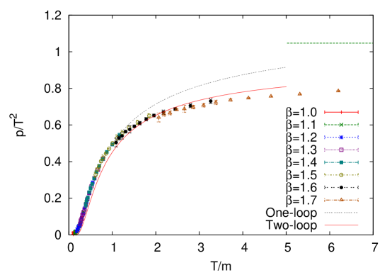
Figure 2: The pressure as a function of $T/m$ in one-loop (blue) and in two-loop (red) approximation compared to lattice simulations for different values of $\beta=N/g^{2}$.

In this subsection we compare the analytic results with lattice simulations. We choose $N=3$, corresponding to a system of three scalar fields. The vacuum mass of the scalar field $m$ is the only dimensionful parameter of the model. Therefore we plot all thermodynamic observables in units of $m.$

Figure 1 shows the analytic result for the temperature dependent renormalized mass of the scalar fields. An important observation is that it has a similar behavior as the gluon mass in the deconfined phase, e.g. ref. [9] and refs. therein. The model exhibits dimensional transmutation just like QCD, meaning that at zero temperature there is a nonvanishing mass gap, which is generated due to renormalization of quantum corrections. Besides, at high $T$ the temperature dependence of the mass can be approximately parametrized by $T/\log T.$ This is exactly the same behavior that one observes for the gluon mass in the deconfined phase.

Figure 2 shows the thermodynamic pressure. The uncertainties are very small and completely overcome by systematics. The high temperature limit is better described in the two-loop calculations, whereas at low temperatures there is a better correspondence between the lattice simulations and the one-loop calculations. We find that at very high temperatures one degree of freedom becomes effectively removed, and the pressure approaches the limit of a non-interacting gas of $N-1$ bosons, $P/N=(N-1)\pi T^{2}/6N,$ which is indicated by the straight dashed line in the upper right corner. This is an immediate consequence of the asymptotic freedom and of the nonlinear constraint. One can understand this behavior by remembering that we start with a free Lagrangian for $N$ scalar fields. Introducing the nonlinear condition, $\Phi^{2}=N/g^{2}$, the thermodynamics is constraint on a two dimensional sphere which effectively removes one degree of freedom. Analytically this removal of one degree of freedom can only be described in the 2-loop approximation.

References

- [1] V. A. Novikov, M. A. Shifman, A. I. Vainshtein and V. I. Zakharov, Phys. Rept. 116, 103 (1984) [Sov. J. Part. Nucl. 17, 204 (1986)] [Fiz. Elem. Chast. Atom. Yadra 17, 472 (1986)].
- [2] C. Rim and W. I. Weisberger, ITP-SB-84-16.
- [3] H. Flyvbjerg, Phys. Lett. B 245, 533 (1990).
- [4] R. G. Root, Phys. Rev. D 10, 3322 (1974).
- [5] J. O. Andersen, D. Boer and H. J. Warringa, Phys. Rev. D 70, 116007 (2004) [hep-ph/0408033].
- [6] E. Seel, S. Struber, F. Giacosa and D. H. Rischke, arXiv:1108.1918 [hep-ph].
- [7] F. Giacosa, S. Lottini, E. Seel, D. Smith, ”Thermodynamics of 2-dim O(N) sigma model: lattice versus 2PI”, to be published.
- [8] G. Boyd, J. Engels, F. Karsch, E. Laermann, C. Legeland, M. Lutgemeier and B. Petersson, “Thermodynamics of SU(3) lattice gauge theory,” Nucl. Phys. B 469, 419 (1996) [hep-lat/9602007].
- [9] F. Giacosa, Phys. Rev. D 83 (2011) 114002 [arXiv:1009.4588 [hep-ph]]; F. Brau and F. Buisseret, Phys. Rev. D 79 (2009) 114007 [arXiv:0902.4836 [hep-ph]]; A. Peshier, B. Kampfer, O. P. Pavlenko and G. Soff, Phys. Rev. D 54 (1996) 2399; P. Castorina and M. Mannarelli, Phys. Rev. C 75 (2007) 054901 [hep-ph/0701206 [hep-ph]].