Dynamic fluctuations in unfrustrated systems: random walks, scalar fields and the Kosterlitz-Thouless phase

Abstract

We study analytically the distribution of fluctuations of the quantities whose average yield the usual two-point correlation and linear response functions in three unfrustrated models: the random walk, the $d$ dimensional scalar field and the $2d$ XY model. In particular we consider the time dependence of ratios between composite operators formed with these fluctuating quantities which generalize the largely studied fluctuation-dissipation ratio, allowing us to discuss the relevance of the effective temperature notion beyond linear order. The behavior of fluctuations in the aforementioned solvable cases is compared to numerical simulations of the $2d$ clock model with $p=6,12$ states.

I Introduction

While in equilibrium systems the correct weighting of fluctuations has disclosed the basis of modern statistical mechanics, uncovering the properties of non-equilibrium fluctuations remains one of the most challenging and far reaching open questions of statistical physics. However, in spite of recent important developments Bertini , explicit calculations, especially for interacting systems, are limited to a few cases Touchette . While for non-equilibrium stationary states a major advance has been the recognition of a general symmetry of the probability distribution of certain observables, described by the so-called fluctuation theorems Evans , the behavior of fluctuations in slowly relaxing systems such as those undergoing critical dynamics, phase-ordering kinetics, glassy evolution, forced relaxation and others, is much less understood. Traditionally these systems have been characterized in terms of the space and time dependence of two-point correlation functions and responses (see, e.g., the review articles Hoha ; Bray ; Cugliandolo02 ). It has been only relatively recently that interest has moved to the study of fluctuations of these quantities and, in particular, their characterization via higher order correlation and response functions ChamonCugliandolo ; Cocuyo ; noichi2 ; annibsollich ; noivarianze ; noispinglass . These properties should, obviously, give us a more detailed description of the behavior of these highly non-trivial processes. A large activity around the analysis of fluctuations in glass forming liquids and other similar materials exists book-fluct .

In this paper we study analytically the distribution of fluctuations of some quantities the average of which yield the usual two-point correlation function and linear response in three unfrustrated models: the random walk, the $d$ dimensional scalar field and the $2d$ XY model. In its structure this paper follows the presentation in cuglia94 where aging and the usual fluctuation-dissipation (FD) relation were studied in these same three models with the purpose of highlighting the fact that neither disorder nor glassiness are needed to obtain non-trivial dynamic features. Composite operators formed with the above-mentioned fluctuating quantities are related to higher order correlation and response functions noichi2 ; noivarianze ; noispinglass ; Secumo , and ratios between such composite operators can then be defined which generalize the largely studied FD ratios. The analysis of these ratios in the asymptotic time limit inform us, in particular, on the relevance of the effective temperature notion Cukup (for reviews see Crri ; Coliza ; Cugliandolo11 ) beyond the linear order. These analytical studies are complemented by numerical simulations of the $2d$ clock model with $p=6$ and $p=12$ states, where a similar behavior is found.

The paper is organized as follows. In Sec. II we define the quantities that we will compute. Section III is devoted to the analysis of Brownian motion in the over-damped limit. In Sec. IV we solve the Langevin dynamics of the scalar field model in $d$ dimensions. In Sec. V we study the evolution of the clock model and its limit, the XY model, in two dimensions where a Kosterlitz-Thouless (KT) phase exists in which the models are critical. Finally, in Sec. VI we present our conclusions.

II Fluctuating quantities

We wish to characterize the statistics of fluctuating quantities the average of which yield the two-time correlation and linear response. The choice of these fluctuating quantities is not unique and their meaningful definition depends on the problem of interest, as we will discuss below. In the simpler cases (as the random walk of Sec. III or the scalar field considered in Sec. IV) one is usually interested in the correlation and response of a field whose dynamics is ruled by a Langevin equation of the type

$$\frac{\partial\phi(\vec{x},t)}{\partial t}=-\Gamma\frac{\delta{\cal F}(\{\phi\})}{\delta\phi(\vec{x},t)}+\xi(\vec{x},t),$$ (1)

${\cal F}$ being an effective Ginzburg-Landau free-energy and $\xi$ a thermal noise with the usual properties $\langle\xi(\vec{x},t)\rangle=0$ and $\langle\xi(\vec{x},t)\xi(\vec{x}^{\prime},t^{\prime})\rangle=2T\delta(\vec{x}-\vec{x}^{\prime})\delta(t-t^{\prime})$ (we set $k_{B}=1$ and we absorbed the coefficient $\Gamma$ with a redefinition of time). This equation is complemented by the choice of an initial condition $\phi(\vec{x},t=0)$.

In this stochastic dynamic equation there are two sources of fluctuations: the initial condition, if taken from a probability distribution, and the random force mimicking the thermal noise. In the process of computing a response function, the applied perturbation may be an additional source of fluctuations, if it is taken to be random. In the analytical approaches contained in this paper we will choose to work with fixed initial conditions and we will therefore freeze the first source of fluctuations mentioned above. The effect of random initial conditions will be considered in Sec. V.2.2 for a discrete model, the clock model, which cannot be described in terms of a Langevin equation and must be studied numerically.

Let us now introduce the two-time average quantities we will be interested in, the correlation and the linear response function, and their fluctuating parts. The two-time correlation function is defined as

$$C\equiv C(\vec{x},\vec{x}^{\prime};t,t^{\prime})=\langle\phi(\vec{x},t)\phi(\vec{x}^{\prime},t^{\prime})\rangle\;,$$ (2)

where $\vec{x}$ and $\vec{x}^{\prime}$ are two generic points in space and $t$ and $t^{\prime}$ two generic times. From this expression the definition of the fluctuating part of the correlation as

$$\widehat{C}\equiv\widehat{C}(\vec{x},\vec{x}^{\prime};t,t^{\prime})=\phi(\vec{x},t)\phi(\vec{x}^{\prime},t^{\prime})\;,$$ (3)

is meaningful, since taking the average of the quantity in Eq. (3) one immediately recognizes the (averaged) correlation $C\equiv C(\vec{x},\vec{x}^{\prime};t,t^{\prime})$. Although the definition (3) is not unique, since other different fluctuating quantities may share the same average, for the correlation function this appears as the most natural choice. Let us notice that not only the average of $\phi(\vec{x},t)\phi(\vec{x}^{\prime},t^{\prime})$ yields $C(\vec{x},\vec{x}^{\prime};t,t^{\prime})$, but composite operators (or moments) formed with this fluctuating field provide higher order correlation functions. This observation, which may seem quite trivial for the correlation function, is not so obvious when dealing with the response function, for which the definition of a fluctuating part is less straightforward. The usual perturbation used to compute it is a field, say $h$, possibly drawn from a probability distribution, that couples linearly to the variable of interest, say $\phi$ itself, in such a way that ${\cal F}\to{\cal F}-\int d^{d}x\ h(\vec{x},t)\phi(\vec{x},t)$. The perturbed Langevin equation then acquires an additional additive force. From here one can easily prove Cugliandolo02 ; Cugliandolo11 ; cuglia94 , for any ${\cal F}$, that the averaged linear response function is simply related to the correlation between $\phi$ and the noise $\xi$:

$$R(\vec{x},\vec{x}^{\prime};t,t^{\prime})=\left.\frac{\delta\langle\phi_{h}(\vec{x},t)\rangle}{\delta h(\vec{x}^{\prime},t^{\prime})}\right|_{h=0}=\frac{1}{2T}\langle\phi(\vec{x},t)\xi(\vec{x}^{\prime},t^{\prime})\rangle\;.$$ (4)

This relation gives us two fluctuating fields, $\frac{\delta\phi_{h}(\vec{x},t)}{\delta h(\vec{x}^{\prime},t^{\prime})}|_{h=0}$ and $\phi(\vec{x},t)\xi(\vec{x}^{\prime},t^{\prime})/(2T)$, whose noise averages yield the linear response function, as natural candidates to define the fluctuating part. The question then arises as to which is, between these two, the most interesting quantity to consider. In fact, although these objects have the same thermal average, they may have different fluctuation spectra and higher-order correlations. In noispinglass we showed that the two-time fields appearing in the Martin-Siggia-Rose-Jenssen-deDominicis dynamic generating functional are naturally related to $\phi(\vec{x},t)\xi(\vec{x}^{\prime},t^{\prime})/(2T)$. This suggests that the quantity $\phi(\vec{x},t)\xi(\vec{x}^{\prime},t^{\prime})/(2T)$ may play a special physical role and is worth of being studied. Indeed, special and interesting properties are exhibited by this fluctuating quantity in the case of aging spin-glasses noispinglass . Similar considerations have led to use this same fluctuating quantity in ferromagnetic systems in noivarianze . Furthermore, it must be recalled that composite operators formed with the field $\phi(\vec{x},t)\xi(\vec{x}^{\prime},t^{\prime})/(2T)$ are directly related to higher order response functions noichi2 ; noivarianze ; noispinglass ; Secumo , a property analogous to the one discussed above for the fluctuating part of the correlation function. This allows one to define ratios between composite operators of the fluctuating parts of response and correlation (see Sec. II.2), which are natural generalizations of the usual FD ratio and, by studying their behavior, to discuss the relevance of the notion of an effective temperature beyond linear order. Finally, restricting to the quadratic models considered analytically in this paper, the quantity $\frac{\delta\phi_{h}(\vec{x},t)}{\delta h(\vec{x}^{\prime},t^{\prime})}|_{h=0}$ is deterministic, while $\phi(\vec{x},t)\xi(\vec{x}^{\prime},t^{\prime})/(2T)$ has a non-trivial fluctuating pattern. Indeed, considering as an example a free-energy functional of the form ${\cal F}=\int d^{d}x\ (\nabla\phi)^{2}/2$ (but the argument is general for any quadratic form), one has that the solution of Eq. (1) is

$$\phi_{h}(\vec{k},t)=\phi(\vec{k},0)e^{-k^{2}t}+\int_{0}^{t}dt^{\prime}\ e^{-k^{2}(t-t^{\prime})}\ [\xi(\vec{k},t^{\prime})+h(\vec{k},t^{\prime})]$$ (5)

from which one immediately concludes that

$$\frac{\delta\phi_{h}(\vec{k},t)}{\delta h(\vec{k}^{\prime},t^{\prime})}=e^{-k^{2}(t-t)}\theta(t-t^{\prime})$$ (6)

is a deterministic function, independent of the initial condition, the applied field and the thermal noise realization. Instead, $\phi(\vec{k},t)\xi(\vec{k}^{\prime},t^{\prime})/(2T)$ fluctuates and its higher order moments are non-trivial, as we will show in the following.

In conclusion, we define the fluctuating part of the linear response as

$$\widehat{R}\equiv\widehat{R}(\vec{x},\vec{x}^{\prime};t,t^{\prime})=\phi(\vec{x},t)\frac{\xi(\vec{x}^{\prime},t^{\prime})}{2T}\;,$$ (7)

which, together with Eq. (3), provide the definitions of fluctuations of the two-time quantities that will be adopted throughout this paper.

In the following we will also consider the time-derivative of $\widehat{C}$:

$$\partial_{t^{\prime}}\widehat{C}=\frac{\partial\widehat{C}}{\partial t^{\prime}}(\vec{x},\vec{x}^{\prime};t,t^{\prime})\;,$$ (8)

and the integrated fluctuating linear response function

$$\widehat{\mu}=\widehat{\mu}(\vec{x},\vec{x}^{\prime};t,t^{\prime},t^{\prime\prime})=\phi(\vec{x},t)\int_{t^{\prime}}^{t^{\prime\prime}}\frac{\xi(\vec{x}^{\prime},z)}{2T}\,dz\;.$$ (9)

With the choice $t^{\prime\prime}=t$ the average of the latter quantity provides the dynamic (sometimes denoted as zero field cooled) susceptibility

$$\chi(\vec{x},\vec{x}^{\prime};t,t^{\prime})=\langle\widehat{\chi}(\vec{x},\vec{x}^{\prime};t,t^{\prime})\rangle=\int_{t^{\prime}}^{t}ds\ \widehat{R}(\vec{x},\vec{x}^{\prime};t,s)\;.$$ (10)

For the $2d$ XY model we will define the relevant fluctuating quantities in Sec. V.

II.1 Joint probability distribution

In simple models with a quadratic Hamiltonian ${\cal H}$, the probability distribution of the fluctuating quantities introduced above can be explicitly exhibited, and a full characterization of the fluctuation spectra can be given (for the $2d$ XY model an equivalent delineation will be provided by studying the moments of any order in Sec. V). Let us start with the simplest case of a single time-dependent function $\phi(t)$ (i.e. we consider a zero space dimensional problem; namely, there is no $\vec{x}$ dependence). It is convenient to introduce the quantities

$$\Phi(t^{\prime\prime},t^{\prime})=\phi(t^{\prime\prime})-\phi(t^{\prime})\;,$$ (11)

and

$$\Xi(t^{\prime\prime},t^{\prime})=\int_{t^{\prime}}^{t^{\prime\prime}}\xi(z)\,dz\;.$$ (12)

In terms of these quantities the variation of the correlation $\Delta\widehat{C}=\widehat{C}(t,t^{\prime\prime})-\widehat{C}(t,t^{\prime})$ and the integrated response function $\widehat{\mu}$ read

$$\Delta\widehat{C}(t,t^{\prime\prime},t^{\prime})=\phi(t)\,\Phi(t^{\prime\prime},t^{\prime})\;,$$ (13)

and

$$\widehat{\mu}(t,t^{\prime\prime},t^{\prime})=\frac{\phi(t)\,\Xi(t^{\prime\prime},t^{\prime})}{2T}\;.$$ (14)

(With an abuse of language we omit to call “fluctuating” the hat quantities.) Notice also that the differential quantities $\partial_{t^{\prime}}\widehat{C}$ and $\widehat{R}$ can be obtained from these forms as $\partial_{t^{\prime}}\widehat{C}=\lim_{\delta\to 0}\Delta\widehat{C}/\delta$ and $\widehat{R}=\lim_{\delta\to 0}\widehat{\mu}/\delta$, where $\delta=t^{\prime\prime}-t^{\prime}$. The joint probability distribution ${\cal P}(\phi,\Phi,\Xi)$ of having $\phi$ at time $t$, $\Phi$ at times $t^{\prime}$ and $t^{\prime\prime}$, and $\Xi$ also at times $t^{\prime}$ and $t^{\prime\prime}$ is Gaussian and reads

$${\cal P}(\phi,\Phi,\Xi)=(2\pi)^{-\frac{3}{2}}\,|G|^{-\frac{1}{2}}\exp\left[-\left(\begin{array}[]{ccc}\phi&\Phi&\Xi\end{array}\right)G^{-1}\left(\begin{array}[]{c}\phi\\ \Phi\\ \Xi\end{array}\right)\right]$$ (15)

where $G$ is the matrix of correlations:

$$G=\left(\begin{array}[]{ccc}\langle\phi^{2}\rangle&\frac{1}{2}\Delta C&\frac{1}{2}\mu\\ \frac{1}{2}\Delta C&\langle\Phi^{2}\rangle&\frac{1}{2}\langle\Phi\Xi\rangle\\ \frac{1}{2}\mu&\frac{1}{2}\langle\Phi\Xi\rangle&\langle\Xi^{2}\rangle\end{array}\right),$$ (16)

$|G|$ its determinant, $\langle\phi^{2}\rangle=C(t,t)$ is the field correlator, $\langle\Phi^{2}\rangle=C(t^{\prime\prime},t^{\prime\prime})+C(t^{\prime},t^{\prime})-2C(t^{\prime\prime},t^{\prime})$ is the field “displacement”, $\Delta C=\langle\Delta\widehat{C}(t,t^{\prime\prime},t^{\prime})\rangle=C(t,t^{\prime\prime})-C(t,t^{\prime})$ and $\mu=\langle\widehat{\mu}\rangle=\int_{t^{\prime}}^{t^{\prime\prime}}dz\ R(t,z)$ in the time-integrated linear response. For white noise $\langle\Xi^{2}\rangle=2T(t^{\prime\prime}-t^{\prime})$. Let us observe that, by choosing $\phi,\Phi,\Xi$ as arguments of ${\cal P}$ one has the advantage of having all finite entries in $G$ [this is not ensured if one uses, for instance, $\phi(t)$, $\phi(t^{\prime})$ and $\xi(t^{\prime})$].

In terms of ${\cal P}$, the joint correlation-response probability distribution $P(\Delta\widehat{C},\widehat{\mu})$ reads

$$P(\Delta\widehat{C}\,,\,\widehat{\mu})=\int d\phi\,d\Phi\,d\,\Xi\,\,{\cal P}(\phi,\Phi,\Xi)\,\delta[\phi\,\Phi-\epsilon\Delta\widehat{C}]\,\delta[\phi\,\Xi-2T\epsilon\widehat{\mu}]\;.$$ (17)

Notice that we have introduced the parameter $\epsilon$ which allows us to use a single form for the probability $P(\Delta\widehat{C},\widehat{\mu})$ of the integrated quantities, by simply setting $\epsilon=1$ in Eq. (17), and the probability $P(\partial_{t^{\prime}}\widehat{C},\widehat{R})$ of the differential ones by letting $\epsilon=\delta$ and taking the limit $\delta\to 0$, namely

$$P(\partial_{t^{\prime}}\widehat{C},\widehat{R})=\left[\lim_{\delta\to 0}\left.P(\Delta\widehat{C},\widehat{\mu})\right|_{\epsilon=\delta}\right]_{\stackrel{{\scriptstyle\widehat{\mu}=\widehat{R}}}{{\Delta\widehat{C}=\partial_{t^{\prime}}\widehat{C}}}}.$$ (18)

Using the integral representation $\delta(x)=(2\pi)^{-1}\int_{-\infty}^{\infty}d\eta\,e^{-i\eta x}$ of the Dirac function one arrives at

$$P(\Delta\widehat{C}\,,\,\widehat{\mu}) = (2\pi)^{-\frac{3}{2}}\,|G|^{-\frac{1}{2}}\int d\phi\,d\Phi\,d\Xi\;\int_{-\infty+i\eta^{*}}^{\infty+i\eta^{*}}\frac{d\eta}{2\pi}\,\int_{-\infty+i\lambda^{*}}^{\infty+i\lambda^{*}}\frac{d\lambda}{2\pi}\,e^{-i(\eta\,\epsilon\Delta\widehat{C}+2\lambda T\epsilon\,\widehat{\mu})}$$ (23)

$$\qquad\qquad\qquad\qquad\qquad\qquad\times\exp\left[-\left(\begin{array}[]{ccc}\phi&\Phi&\Xi\end{array}\right)B_{\eta\lambda}^{-1}\left(\begin{array}[]{c}\phi\\ \Phi\\ \Xi\end{array}\right)\right]$$

with

$$B_{\eta\lambda}^{-1}=G^{-1}+\left(\begin{array}[]{ccc}0&-i\frac{\eta}{2}&-i\frac{\lambda}{2}\\ -i\frac{\eta}{2}&0&0\\ -i\frac{\lambda}{2}&0&0\end{array}\right).$$ (24)

Notice that, following standard techniques BerlinKac , the integration paths in Eq. (23) have been deformed by the arbitrary shifts $\eta^{*}$ and $\lambda^{*}$. This does not change the value of the integral since it merely amounts to introducing an additive term $\eta^{*}(\phi\Phi-\epsilon\Delta\widehat{C})+\lambda^{*}(\phi\Xi-2T\epsilon\widehat{\mu})$, which vanishes due to the $\delta$-constraints in Eq. (17), in the argument of the exponential on the right-hand-side (rhs) of Eq. (23). In turn, a properly deformed integration path may render the integrations over $d\phi\,d\Phi\,d\Xi$ convergent in the cases in which (like in Sec. IV.1) the result over the orginal route is divergent (when the integrations over $d\phi\,d\Phi\,d\Xi$ are taken before those over $d\eta\,d\lambda$).

Performing the Gaussian integrations in Eq. (23) one obtains

$$P(\Delta\widehat{C}\,,\,\widehat{\mu}) = \!\!|G|^{-\frac{1}{2}}\int_{-\infty+i\eta^{*}}^{\infty+i\eta^{*}}\frac{d\eta}{2\pi}\,\int_{-\infty+i\lambda^{*}}^{\infty+i\lambda^{*}}\frac{d\lambda}{2\pi}\,\,e^{-i(\eta\,\epsilon\Delta\widehat{C}+2\lambda T\epsilon\,\widehat{\mu})}\ |B_{\eta\lambda}|^{\frac{1}{2}}\,\,$$ (25)

$$= \!\!\int_{-\infty+i\eta^{*}}^{\infty+i\eta^{*}}\frac{d\eta}{2\pi}\,\int_{-\infty+i\lambda^{*}}^{\infty+i\lambda^{*}}\frac{d\lambda}{2\pi}\,\,e^{-i(\eta\,\epsilon\Delta\widehat{C}+2\lambda T\epsilon\,\widehat{\mu})}\left\{1-\frac{1}{2}i\eta\Delta C-\frac{1}{2}i\lambda(2T\mu)\right.$$

$$\left.\qquad\qquad-\frac{1}{8}\eta\lambda[2T\mu\Delta C-2\langle\phi^{2}\rangle\langle\Phi\Xi\rangle]-\frac{1}{16}\eta^{2}[(\Delta C)^{2}-4\langle\phi^{2}\rangle\langle\Phi^{2}\rangle]\right.$$

$$\left.\qquad\qquad-\frac{1}{16}\lambda^{2}[(2T\mu)^{2}-4\langle\phi^{2}\rangle\langle\Xi^{2}\rangle]\right\}^{-\frac{1}{2}}.$$

Note that the three time-dependencies ($t>t^{\prime\prime}>t^{\prime}$) enter only via averages. We will explicitly compute $P$ in a specific zero-dimensional model, the random walk, in Sec. III.1.

Let us now generalize what done insofar to a scalar field $\phi(\vec{x},t)$ defined on a $d+1$ dimensional space. Taking into account the space dependence the definitions (11) and (12) are replaced by

$$\Phi(\vec{x}^{\prime},t^{\prime\prime},t^{\prime})=\phi(\vec{x}^{\prime},t^{\prime\prime})-\phi(\vec{x}^{\prime},t^{\prime})\;,$$ (26)

and

$$\Xi(\vec{x}^{\prime},t^{\prime\prime},t^{\prime})=\int_{t^{\prime}}^{t^{\prime\prime}}\xi(\vec{x}^{\prime},z)\,dz\;.$$ (27)

The fluctuating quantities we are interested in are

$$\Delta\widehat{C}(\vec{r}=\vec{x}-\vec{x}^{\prime},t,t^{\prime\prime},t^{\prime}) = \int d\vec{x}\ \phi(\vec{x},t)\Phi(\vec{x}^{\prime},t^{\prime\prime},t^{\prime})$$ (28)

$$= \int\frac{d\vec{k}}{(2\pi)^{d}}\,\widetilde{\phi}(\vec{k},t)\widetilde{\Phi}(-\vec{k},t^{\prime\prime},t^{\prime})\,e^{i\vec{k}(\vec{x}-\vec{x}^{\prime})}\,\,,$$

and

$$\widehat{\mu}(\vec{r}=\vec{x}-\vec{x}^{\prime},t,t^{\prime\prime},t^{\prime}) = \frac{1}{2T}\int d\vec{x}\ \phi(\vec{x},t)\Xi(\vec{x}^{\prime},t^{\prime\prime},t^{\prime})$$ (29)

$$= \frac{1}{2T}\int\frac{d\vec{k}}{(2\pi)^{d}}\,\widetilde{\phi}(\vec{k},t)\widetilde{\Xi}(-\vec{k},t^{\prime\prime},t^{\prime})\,e^{i\vec{k}(\vec{x}-\vec{x}^{\prime})}\,\,,$$

where $\widetilde{\phi}(\vec{k},t)$ is the $\vec{k}$ component of the Fourier transform  of the field $\phi(\vec{x},t)$, and similarly for $\widetilde{\Phi}$ and $\widetilde{\Xi}$. From here onwards $\vec{r}\equiv\vec{x}-\vec{x}^{\prime}$. When the $\vec{k}$ components are independent (i.e., for a quadratic Hamiltonian), the joint probability $P(\phi,\Phi,\Xi)$ is factorized as

$${\cal P}(\widetilde{\phi},\widetilde{\Phi},\widetilde{\Xi})=\prod_{k}(2\pi)^{-\frac{3}{2}}\,|\widetilde{G}|^{-\frac{1}{2}}\exp\left[-\left(\begin{array}[]{ccc}\widetilde{\phi}&\widetilde{\Phi}&\widetilde{\Xi}\end{array}\right)\widetilde{G}^{-1}\left(\begin{array}[]{c}\widetilde{\phi}\\ \widetilde{\Phi}\\ \widetilde{\Xi}\end{array}\right)\right]$$ (30)

where $\left(\begin{array}[]{ccc}\widetilde{\phi}&\widetilde{\Phi}&\widetilde{\Xi}\end{array}\right)$ and $\left(\begin{array}[]{c}\widetilde{\phi}\\ \widetilde{\Phi}\\ \widetilde{\Xi}\end{array}\right)$ are evaluated at the wavevectors $\vec{k}$ and $-\vec{k}$, respectively. $\widetilde{G}$ is the matrix of the $\vec{k}$-component correlations

$$\widetilde{G}=\left(\begin{array}[]{ccc}\widetilde{C}_{\phi\phi}&\frac{1}{2}\Delta\widetilde{C}&\frac{1}{2}\widetilde{\mu}\\ \frac{1}{2}\Delta\widetilde{C}&\widetilde{C}_{\Phi\Phi}&\frac{1}{2}\widetilde{C}_{\Phi\Xi}\\ \frac{1}{2}\widetilde{\mu}&\frac{1}{2}\widetilde{C}_{\Phi\Xi}&\widetilde{C}_{\Xi\Xi}\end{array}\right)\,\,,$$ (31)

with $\Delta\widetilde{C}=\widetilde{C}(\vec{k},t,t^{\prime\prime})-\widetilde{C}(\vec{k},t,t^{\prime})$, where

$$(2\pi)^{d}\delta(\vec{k}+\vec{k}^{\prime})\widetilde{C}(\vec{k},t,t^{\prime})=\langle\phi(\vec{k},t)\phi(\vec{k}^{\prime},t^{\prime})\rangle,$$ (32)

is the usual two-time structure factor. The other elements of the $\widetilde{G}$ matrix, which as in the zero-dimensional case are all finite, are the correlators $(2\pi)^{d}\delta(\vec{k}+\vec{k}^{\prime})\widetilde{\mu}(\vec{k},t,t^{\prime\prime},t^{\prime})=\langle\phi(\vec{k},t)\Xi(\vec{k}^{\prime},t^{\prime\prime},t^{\prime})\rangle$, $(2\pi)^{d}\delta(\vec{k}+\vec{k}^{\prime})\widetilde{C}_{\Phi\Xi}(\vec{k},t,t^{\prime\prime},t^{\prime})=\langle\widetilde{\Phi}(\vec{k},t^{\prime\prime},t^{\prime})\widetilde{\Xi}(\vec{k}^{\prime},t^{\prime\prime},t^{\prime})\rangle$, and similarly for $\widetilde{C}_{\phi\phi}$, $\widetilde{C}_{\Phi\Phi}$, and $\widetilde{C}_{\Xi\Xi}$.

Starting from this, the joint probability distribution $P(\Delta\widehat{C},\widehat{\mu})$ of the real-space quantities defined in Eqs. (28) and (29) can be straightforwardly obtained proceeding along the same lines as for the zero-dimensional case. We first introduce the matrix $B_{\eta\lambda}$ which is related to $\widetilde{G}$ by

$$B_{\eta\lambda}^{-1}(\vec{k},\vec{r}=\vec{x}-\vec{x}^{\prime})=\widetilde{G}^{-1}(\vec{k})+\left(\begin{array}[]{ccc}0&-i\frac{\eta}{2}e^{i\vec{k}(\vec{x}-\vec{x}^{\prime})}&-i\frac{\lambda}{2}e^{i\vec{k}(\vec{x}-\vec{x}^{\prime})}\\ -i\frac{\eta}{2}e^{i\vec{k}(\vec{x}-\vec{x}^{\prime})}&0&0\\ -i\frac{\lambda}{2}e^{i\vec{k}(\vec{x}-\vec{x}^{\prime})}&0&0\end{array}\right)\,\,,$$ (33)

and is the generalization of Eq. (24). We next obtain

$$P(\Delta\widehat{C}\,,\,\widehat{\mu}) = \int_{-\infty+i\eta^{*}}^{\infty+i\eta^{*}}\frac{d\eta}{2\pi}\,\int_{-\infty+i\lambda^{*}}^{\infty+i\lambda^{*}}\frac{d\lambda}{2\pi}\,\,\exp\left[-i(\eta\,\epsilon\Delta\widehat{C}+2\lambda T\epsilon\,\widehat{\mu})+\frac{V}{2}\int\frac{d\vec{k}}{(2\pi)^{d}}\ln\left(\frac{|B_{\eta\lambda}(\vec{k},\vec{r})|}{|G(\vec{k})|}\right)\right]$$ (34)

$$= \int_{-\infty+i\eta^{*}}^{\infty+i\eta^{*}}\frac{d\eta}{2\pi}\,\int_{-\infty+i\lambda^{*}}^{\infty+i\lambda^{*}}\frac{d\lambda}{2\pi}\,\,\exp\left[-i(\eta\,\epsilon\Delta\widehat{C}+2\lambda T\epsilon\,\widehat{\mu})\right]$$

$$\qquad\qquad\times\exp\left\{-\frac{V}{2}\int\frac{d\vec{k}}{(2\pi)^{d}}\ln\left(1-\frac{1}{2}i\eta e^{i\vec{k}\vec{r}}\Delta\widetilde{C}-\right.\right.$$

$$\qquad\qquad\qquad\frac{1}{2}i\lambda e^{i\vec{k}\vec{r}}(2T\widetilde{\mu})-\frac{1}{8}\eta\lambda e^{2i\vec{k}\vec{r}}[2T\widetilde{\mu}\Delta\widetilde{C}-2\widetilde{C}_{\phi\phi}\widetilde{C}_{\Phi\Xi}]-$$

$$\qquad\qquad\qquad\frac{1}{16}\eta^{2}e^{2i\vec{k}\vec{r}}[(\Delta\widetilde{C})^{2}-4\widetilde{C}_{\phi\phi}\widetilde{C}_{\Phi\Phi}]-\left.\left.\frac{1}{16}\lambda^{2}e^{2i\vec{k}\vec{r}}[(2T\widetilde{\mu})^{2}-4\widetilde{C}_{\phi\phi}\widetilde{C}_{\Xi\Xi}]\right)\right\},$$

where $V$ is the volume of the system, which extends Eq. (25) to the finite dimensional case. This form is totally general (for a quadratic Hamiltonian). Note that the three time dependencies ($t>t^{\prime\prime}>t^{\prime}$) still enter only via averages, as in the zero-dimensional case, while the $\vec{r}$- (actually $r$-) dependence is explicit. We will discuss the properties of $P$ in a specific $d$-dimensional model, the scalar field, in Sec. IV.1.

II.2 Composite operators

We now go on by using the generic notation and we build averages of composite fields of the form

$${\cal D}^{(n,m)}=\langle\prod_{i=m+1}^{n}\partial_{t^{\prime}_{i}}\widehat{C}_{i}\,\prod_{j=1}^{m}\widehat{R}_{j}\;\rangle\;,$$ (35)

where we have used the shorthand

$$\widehat{C}_{i}=\widehat{C}(\vec{x}_{i},\vec{x}^{\prime}_{i};t_{i},t^{\prime}_{i})$$ (36)

and similarly for $R_{i}$, where $\vec{x}_{i}$ and $\vec{x}^{\prime}_{i}$ ($t_{i}$ and $t^{\prime}_{i}$) are two generic space positions (times), with $t_{i}\geq t^{\prime}_{i}$.

It is also interesting to use the quantity in which the fluctuating time-variation of the correlation and linear response have been time-integrated:

$${\cal C}^{(n,m)}=\langle\prod_{i=m+1}^{n}\widehat{C}_{i}\,\prod_{j=1}^{m}\widehat{\chi}_{j}\;\rangle\;.$$ (37)

Moments are obtained from these quantities by subtracting a suitable disconnected part, as will be discussed in Sec. V.1.4. The averaged correlation, linear response and the integrated linear response are simply ${\cal C}^{(1,0)}$, ${\cal D}^{(1,1)}$ and ${\cal C}^{(1,1)}$, respectively. Analogously, for $n>1$ the quantities ${\cal C}^{(n,0)}$ (or ${\cal D}^{(n,0)}$) are higher order correlation functions (or their time derivatives) and, similarly, as discussed in noichi2 ; noivarianze ; noispinglass ; Secumo , ${\cal C}^{(n,n)}$ and ${\cal D}^{(n,n)}$ are related to higher order response functions (time integrated or impulsive, respectively) .

Notice that the quantities in Eqs. (35) and (37) cannot be obtained from the joint probability distribution computed in Sec. II.1: indeed, in general, they involve correlations and responses evaluated at different space-time variables $\vec{x}_{i},\vec{x}^{\prime}_{i};t_{i},t^{\prime}_{i}$ for any $i$, whereas both $\Delta\widehat{C}$ and $\widehat{\mu}$ in Eqs. (28) and (29) are considered with the same space-time arguments (namely, $\vec{x},\vec{x}^{\prime}$ and $t,t^{\prime},t^{\prime\prime}$).

Let us now define the generalized FD ratio as

$$X^{(n;m,m^{\prime})}\equiv T^{m-m^{\prime}}\,\frac{{\cal D}^{(n,m)}}{{\cal D}^{(n,m^{\prime})}}\;.$$ (38)

Letting $n=1$, $m=1$, $m^{\prime}=0$ one recovers the usual FD ratio $X$. These quantities do not put higher order FDTs to the test directly as these are complicated functions, involving several terms Secumo ; noichi2 , but they do evaluate whether all these terms scale in the same way thus allowing for the existence of an effective temperature taking finite values over non-trivial time regimes.

III Brownian motion

The overdamped Langevin dynamics of a Brownian particle is ruled by Eq. (1) with a single function $\phi$ (i.e. there is no dependence on $\vec{x}$) and ${\cal H}\equiv 0$. In this case $\phi$ should be interpreted as the position of a Brownian particle on a line. The extension to the case of a vector $\vec{\phi}$ with $d$ components, describing diffusion in $d$ dimensions, is trivial and the basic results remain unaltered.

III.1 Joint probability distribution

In this simple problem one trivially has $\Phi\equiv\Xi$. The joint probability distribution (25) of $\Delta\widehat{C}(t,t^{\prime\prime}t,^{\prime})$ and $\widehat{\mu}(t,t^{\prime\prime},t^{\prime})$ then reduces to

$$P(\Delta\widehat{C}\,,\,\widehat{\mu})=\int_{-\infty}^{\infty}\frac{d\eta}{2\pi}\,\int_{-\infty}^{\infty}\frac{d\lambda}{2\pi}\,e^{-i(\eta\,\epsilon\Delta\widehat{C}+2\lambda T\epsilon\,\widehat{\mu})}\,$$

$$\qquad\qquad\qquad\qquad\times\frac{1}{\sqrt{1-\frac{1}{2}i(\eta+\lambda)\Delta C-\frac{1}{16}(\eta+\lambda)^{2}[(\Delta C)^{2}-4\langle\phi^{2}\rangle\langle\Phi^{2}\rangle]}}$$ (39)

with $\Delta C=2T(t^{\prime\prime}-t^{\prime})$, $\langle\phi^{2}\rangle=2Tt$ and $\langle\Phi^{2}\rangle=\langle\Xi^{2}\rangle=2T(t^{\prime\prime}-t^{\prime})$, where we assumed that $t>t^{\prime\prime}>t^{\prime}$ and set $\eta^{*}=\lambda^{*}=0$ since every integral is convergent.

This form is symmetric under the exchange $\Delta\widehat{C}\leftrightarrow 2T\widehat{\mu}$, thus indicating that these two quantities are equally distributed. Indeed, since $\Phi=\Xi$ one has $\Delta\widehat{C}=2T\widehat{\mu}$ and, therefore, the fluctuations of the composite fields whose averages are the correlation and linear response are just identical in this case. As a consequence, all the composite operators of Eq. (35) with the same value of $n$ [with $(t_{i},t^{\prime}_{i})=(t,t^{\prime})$ $\forall i$] scale in the same way (that is to say, they have the same dependence on the times $t,t^{\prime}$). Moreover, introducing $\omega=\eta+\lambda$ one can explicitly integrate expression (39) and find

$$P(\Delta\widehat{C}\,,\,\widehat{\mu})=\delta\left(\epsilon(2T\widehat{\mu}-\Delta\widehat{C})\right)\int_{-\infty}^{\infty}\frac{d\omega}{2\pi}\frac{e^{-i\omega\epsilon\Delta\widehat{C}}}{\sqrt{1-\frac{1}{2}i\omega\Delta C-\frac{1}{16}\omega^{2}[(\Delta C)^{2}-4\langle\phi^{2}\rangle\langle\Phi^{2}\rangle]}}\;.$$ (40)

In the above integral, the integrand has two branch points at $\omega=\omega_{\pm}$, with

$$\omega_{\pm}=4\,\frac{\pm 2\sqrt{\langle\phi^{2}\rangle\langle\Phi^{2}\rangle}-\Delta C}{(\Delta C)^{2}-4\langle\phi^{2}\rangle\langle\Phi^{2}}\;.$$ (41)

Performing the integral we obtain

$$P(\Delta\widehat{C}\,,\,\widehat{\mu})=\frac{4e^{\displaystyle{\frac{4\Delta C\epsilon\Delta\widehat{C}}{4\langle\phi^{2}\rangle\langle\Phi^{2}\rangle-(\Delta C)^{2}}}}}{\pi\sqrt{4\langle\phi^{2}\rangle\langle\Phi^{2}\rangle-(\Delta C)^{2}}}\,K_{0}\left[8\epsilon\frac{\sqrt{\langle\phi^{2}\rangle\langle\Phi^{2}\rangle}}{4\langle\phi^{2}\rangle\langle\Phi^{2}\rangle-(\Delta C)^{2}}\,|\Delta\widehat{C}|\right]\delta\left(\epsilon(2T\widehat{\mu}-\Delta\widehat{C})\right),$$ (42)

where $K_{0}(z)$ is the modified Bessel function which can be expressed as $K_{0}(z)=\int_{1}^{\infty}e^{zx}(x^{2}-1)^{-1/2}$. This result is very close to the one presented in Chcuyo for the probability distribution function (pdf) of the two-time composite field $\phi_{\alpha}(\vec{x},t)\phi_{\alpha}(\vec{x},t^{\prime})$ in the $O(N)$ ferromagnetic model in the large $N$ limit. In both cases, the time dependencies enter only through the correlation functions, $\langle\phi^{2}\rangle(t)=C(t,t)$, $C(t^{\prime\prime},t^{\prime\prime})$, $C(t^{\prime},t^{\prime})$ and $C(t^{\prime\prime},t^{\prime})$.

III.2 Composite operators

The properties of ${\cal D}^{(n,m)}$ can be computed explicitly as

$${\cal D}^{(n;m)} = \langle\ \prod_{i=m+1}^{n}\phi(t_{i})\dot{\phi}(t_{i}^{\prime})\prod_{j=1}^{m}\phi(t_{j})\xi(t_{j}^{\prime})/(2T)\ \rangle$$ (43)

$$= \langle\ \prod_{i=m+1}^{n}\phi(t_{i})\xi(t_{i}^{\prime})\prod_{j=1}^{m}\phi(t_{j})\xi(t_{j}^{\prime})/(2T)\ \rangle$$

$$= \langle\ \prod_{k=1}^{n}\phi(t_{k})\xi(t_{k}^{\prime})\ \rangle\;(2T)^{-m}\;.$$

The remaining average can be expanded in products of two-point correlation and linear response functions by using Wick’s theorem applied to the Gaussian variables $\phi$ and $\xi$. In so doing one finds the explicit $2n$-time dependence of ${\cal D}^{(n,m)}$. If one is interested in the behavior of the generalized FD ratio $X^{(n;m,m^{\prime})}$ this calculation is not necessary since the non-trivial factors in the numerator and denominator cancel out and one simply finds a constant,

$$X^{(n;m,m^{\prime})}=\left(\frac{1}{2}\right)^{m-m^{\prime}}\;,$$ (44)

independently of $n$. For $m=1$ and $m^{\prime}=0$ one recovers $X=1/2$, the usual FD ratio cuglia94 ; Pottier03 of the random walk. Equation (44) generalizes the result of Sec. III.1, showing that moments with different $m$ but the same $n$ scale in the same way for any choice of the time variables.

IV The free scalar field

The Langevin relaxation of the scalar field in $d$ spatial dimensions is given by

$$\frac{\partial\phi(\vec{x},t)}{\partial t}=-\frac{\delta F[\phi]}{\delta\phi(\vec{x},t)}+\xi(\vec{x},t)\;.$$ (45)

In the free-field case the Ginzburg-Landau functional is simply

$$F[\phi]=\frac{1}{2}\int d\vec{x}\ [\nabla\phi(\vec{x},t)]^{2}\;.$$ (46)

The expectations of the thermal noise are the usual ones reported below Eq. (1). Equations (45) and (46) also constitute the Edwards-Wilkinson model for the motion of an interface (with no overhangs) in $d$ transverse dimensions. In the context of interfaces, the fluctuations of a two-time quantity the average of which is the roughness were studied in Bustingorry0 ; Bustingorry ; Iguain ; Pleimling .

The Fourier transformed noise statistics are such that $\langle\xi(\vec{k},t)\rangle=0$ and $\langle\xi(\vec{k},t)\xi(\vec{k}^{\prime},t^{\prime})\rangle$$=2T(2\pi)^{d}\delta(\vec{k}+\vec{k}^{\prime})\delta(\vec{t}-\vec{t}^{\prime})$. Starting from $\phi(\vec{x},0)=0$, without loss of generality, one has

$$\phi(\vec{k},t)=\int_{0}^{t}ds\;e^{-k^{2}(t-s)}\,\xi(\vec{k},s)$$ (47)

and $\phi(\vec{k},t)$ as well as $\phi(\vec{x},t)$ inherit Gaussian statistics from $\xi$. From Eq. (47) for the Fourier space correlator (32) one obtains

$$\widetilde{C}(\vec{k};t,t^{\prime})=\frac{T}{k^{2}}\left[e^{-k^{2}(t-t^{\prime})}-e^{-k^{2}(t+t^{\prime})}\right]\;.$$ (48)

Introducing a short-distance cut-off $a^{2}=1/\Lambda^{2}$ mimicking a lattice spacing, so that $\int d\vec{k}\to\int d\vec{k}\ \exp(-\frac{k^{2}}{\Lambda^{2}})$, the real space correlation function reads

$$C(r;t,t^{\prime})\equiv\langle\,\phi(\vec{x},t)\phi(\vec{x}^{\prime},t^{\prime})\,\rangle=\int\frac{d\vec{k}}{(2\pi)^{d}}\ \widetilde{C}(\vec{k};t,t^{\prime})\ e^{-\frac{k^{2}}{\Lambda^{2}}}\ e^{-i\vec{k}\vec{r}}\;,$$ (49)

with $r=|\vec{x}-\vec{x}^{\prime}|$, and one finds

$$C(r;t,t^{\prime})=\frac{Tr^{2-d}}{4\pi^{d/2}}\,\Gamma\left[\frac{d}{2}-1,\frac{\Lambda^{2}r^{2}}{4[1+\Lambda^{2}(t+t^{\prime})]},\frac{\Lambda^{2}r^{2}}{4[1+\Lambda^{2}(t-t^{\prime})]}\right]\;,$$ (50)

where

$$\Gamma[n,a,b]\equiv\int_{a}^{b}dz\,z^{n-1}e^{-z}$$ (51)

is the generalized incomplete Gamma function. Analogously, the linear response is

$$R(r;t,t^{\prime})\equiv\left.\frac{\delta\langle\phi(\vec{x},t)\rangle_{h}}{\delta h(\vec{x}^{\prime},t^{\prime})}\right|_{h=0} = \langle\phi(\vec{x},t)\xi(\vec{x}^{\prime},t^{\prime})\rangle/(2T)$$ (52)

$$= \frac{\Lambda^{d}}{(4\pi)^{d/2}}\;\frac{e^{-\left[\displaystyle{\frac{\Lambda^{2}r^{2}}{4[1+\Lambda^{2}(t-t^{\prime})]}}\right]}}{\left[1+\Lambda^{2}(t-t^{\prime})\right]^{d/2}}\,\theta(t-t^{\prime})\;.$$

The relevant long-times limit is such that $\Lambda^{2}(t-t^{\prime})\gg 1$. In this limit the partial derivative of Eq. (50) with respect to $t^{\prime}$ becomes

$$\partial_{t^{\prime}}C(r;t,t^{\prime})\simeq\frac{T\Lambda^{d}}{2^{d}\pi^{d/2}}\,t^{\prime-d/2}\left[\left(y-1\right)^{-d/2}e^{-\zeta}+\left(y+1\right)^{-d/2}e^{-\frac{y-1}{y+1}\,\zeta}\right]\;,$$ (53)

(and similarly for $\partial_{t}C$) while from Eq. (52) one has

$$R(r;t,t^{\prime})=\frac{\Lambda^{d}}{2^{d}\pi^{d/2}}\,t^{\prime-d/2}\left(y-1\right)^{-d/2}e^{-\zeta}\,\theta(t-t^{\prime})\;,$$ (54)

where $\zeta=r^{2}/[4(t-t^{\prime})]$ and $y=t/t^{\prime}$. Equations (53) and (54) mean that for $r^{2}\ll 4(t-t^{\prime})$, $R$ and $\partial_{t^{\prime}}C$ scale in the same way, namely $R\simeq t^{\prime-d/2}f_{R}(t/t^{\prime})$ and $\partial_{t^{\prime}}C\simeq t^{\prime-d/2}f_{\partial C}(t/t^{\prime})$, with $f_{R}(y)=\Lambda^{d}[4\pi(y-1)]^{-d/2}$ and $f_{\partial C}(y)=T\Lambda^{d}(4\pi)^{-d/2}[(y-1)^{-d/2}+(y+1)^{-d/2}]$, respectively. In this regime, the FD ratio leticia

$$\lim_{r^{2}\ll(t-t^{\prime})}X(r;t,t^{\prime})=\lim_{r^{2}\ll(t-t^{\prime})}\frac{R(r;t,t^{\prime})}{\partial_{t^{\prime}}C(r;t,t^{\prime})}=\left[1+\left(\frac{y-1}{y+1}\right)^{d/2}\right]^{-1}$$ (55)

is independent of $r$ and converges, for $y\to\infty$, to the limiting value godluck

$$X_{\infty}\equiv\lim_{t/t^{\prime}\to\infty}\ \lim_{r^{2}\ll 2\Lambda^{2}(t-t^{\prime})}X(r;t,t^{\prime})=\frac{1}{2}.$$ (56)

Notice that this asymptotic value does not depend upon the distance for any choice of $r$ [not only for $r^{2}\ll(t-t^{\prime})$] since, for $y\gg 1$, $R$ and $\partial_{t^{\prime}}C$ are proportional in any case:

$$\lim_{t/t^{\prime}\to\infty}X(r;t,t^{\prime})=\frac{1}{2}\;.$$ (57)

This result is the same as the one found for the random walk problem, see Sec. III.

IV.1 Joint probability distribution

In the large volume limit the joint probability (34) can be computed by using saddle point techniques. Changing the integration variables to $z_{C}=i\eta$, $z_{\mu}=i\lambda$, and letting $z^{*}_{C}=i\eta^{*},z^{*}_{\mu}=i\lambda^{*}$, Eq. (34) can be cast as

$$P(\Delta\widehat{C}\,,\,\widehat{\mu})=\int_{-i\infty+z^{*}_{C}}^{i\infty+z^{*}_{C}}\frac{dz_{C}}{2\pi}\,\int_{-i\infty+z^{*}_{\mu}}^{i\infty+z^{*}_{\mu}}\frac{dz_{\mu}}{2\pi}\,\,e^{Vh(\widehat{d}_{C},\widehat{d}_{\mu};\vec{x},\vec{x}^{\prime};t,t^{\prime},t^{\prime\prime},z_{C},z_{\mu})}$$ (58)

where $\widehat{d}_{C}=\frac{\epsilon\Delta\widehat{C}}{V}$, $\widehat{d}_{\mu}=\frac{2T\epsilon\widehat{\mu}}{V}$ are the correlation and response densities, and

$$h(\widehat{d}_{C},\widehat{d}_{\mu};\vec{x},\vec{x}^{\prime};t,t^{\prime},t^{\prime\prime},z_{c},z_{\mu})=-z_{C}\widehat{d}_{C}-z_{\mu}\widehat{d}_{\mu}+G(\vec{x},\vec{x}^{\prime},t,t^{\prime},t^{\prime\prime},z_{C},z_{\mu})$$ (59)

with

$$G(\vec{x},\vec{x}^{\prime},t,t^{\prime},t^{\prime\prime},z_{C},z_{\mu})=-\frac{1}{2}\int\frac{d\vec{k}}{(2\pi)^{d}}\ln H(\vec{k},\vec{x},\vec{x}^{\prime};t,t^{\prime},t^{\prime\prime},z_{C},z_{\mu})$$ (60)

and

$$H(\vec{k},\vec{x},\vec{x}^{\prime};t,t^{\prime},t^{\prime\prime},z_{C},z_{\mu})=1-\frac{1}{2}z_{C}e^{i\vec{k}|\vec{x}-\vec{x}^{\prime}|}\Delta\widetilde{C}-\frac{1}{2}z_{\mu}e^{i\vec{k}|\vec{x}-\vec{x}^{\prime}|}(2T\widetilde{\mu})$$

$$\qquad\qquad\qquad+\frac{1}{8}z_{C}z_{\mu}e^{2i\vec{k}|\vec{x}-\vec{x}^{\prime}|}[2T\widetilde{\mu}\Delta\widetilde{C}-2\widetilde{C}_{\phi\phi}\widetilde{C}_{\Phi\Xi}]+\frac{1}{16}z_{C}^{2}e^{2i\vec{k}|\vec{x}-\vec{x}^{\prime}|}[(\Delta\widetilde{C})^{2}-4\widetilde{C}_{\phi\phi}\widetilde{C}_{\Phi\Phi}]$$

$$\qquad\qquad\qquad+\frac{1}{16}z_{\mu}^{2}e^{2i\vec{k}|\vec{x}-\vec{x}^{\prime}|}[(2T\widetilde{\mu})^{2}-4\widetilde{C}_{\phi\phi}\widetilde{C}_{\Xi\Xi}]\;.$$ (61)

In the large $V$ limit, to any choice of the fluctuating correlation and response $\widehat{d}_{C}$ and $\widehat{d}_{\mu}$ there corresponds a couple of real quantities $z_{C}=z^{*}_{C}$ and $z_{\mu}=z^{*}_{\mu}$ whose contribution dominates the whole double integral in Eq. (58). $z^{*}_{C}(\vec{x},\vec{x}^{\prime},t,t^{\prime},t^{\prime\prime})$ and $z^{*}_{\mu}(\vec{x},\vec{x}^{\prime},t,t^{\prime},t^{\prime\prime})$ are solutions to the coupled system of equation:

$$\left\{\begin{array}[]{rcl}\displaystyle\widehat{d}_{C}&=&\left.\displaystyle\frac{\partial G}{\partial z_{C}}\right|_{z^{*}_{C},z^{*}_{\mu}}\\ &=&\displaystyle\frac{1}{2}\int\frac{d\vec{k}}{(2\pi)^{d}}\frac{\frac{1}{2}e^{i\vec{k}|\vec{x}-\vec{x}^{\prime}|}\Delta\widetilde{C}-\frac{1}{8}e^{2i\vec{k}|\vec{x}-\vec{x}^{\prime}|}[2T\widetilde{\mu}\Delta\widetilde{C}-2\widetilde{C}_{\phi\phi}\widetilde{C}_{\Phi\Xi}]z^{*}_{\mu}-\frac{1}{8}e^{2i\vec{k}|\vec{x}-\vec{x}^{\prime}|}[(\Delta\widetilde{C})^{2}-4\widetilde{C}_{\phi\phi}\widetilde{C}_{\Phi\Phi}]z^{*}_{C}}{H(\vec{k},\vec{x},\vec{x}^{\prime},t,t^{\prime},t^{\prime\prime},z^{*}_{C},z^{*}_{\mu})}\;,\\ \displaystyle\widehat{d}_{\mu}&=&\left.\displaystyle\frac{\partial G}{\partial z_{\mu}}\right|_{z^{*}_{C},z^{*}_{\mu}}\\ &=&\displaystyle\frac{1}{2}\int\frac{d\vec{k}}{(2\pi)^{d}}\frac{\frac{1}{2}e^{i\vec{k}|\vec{x}-\vec{x}^{\prime}|}2T\widetilde{\mu}-\frac{1}{8}e^{2i\vec{k}|\vec{x}-\vec{x}^{\prime}|}[2T\widetilde{\mu}\Delta\widetilde{C}-2\widetilde{C}_{\phi\phi}\widetilde{C}_{\Phi\Xi}]z^{*}_{C}-\frac{1}{8}e^{2i\vec{k}|\vec{x}-\vec{x}^{\prime}|}[(2T\widetilde{\mu})^{2}-4\widetilde{C}_{\phi\phi}\widetilde{C}_{\Xi\Xi}]z^{*}_{\mu}}{H(\vec{k},\vec{x},\vec{x}^{\prime},t,t^{\prime},t^{\prime\prime},z^{*}_{C},z^{*}_{\mu})}\;.\end{array}\right.$$ (66)

Once these equations are solved to find $z^{*}_{C}$ and $z^{*}_{\mu}$ the joint probability distribution for large $V$ can be written as

$$P(\Delta\widehat{C}\,,\,\widehat{\mu})=\frac{1}{(2\pi)^{2}}\,\,e^{Vh(\widehat{d}_{C},\widehat{d}_{\mu};\vec{x},\vec{x}^{\prime};t,t^{\prime},t^{\prime\prime},z^{*}_{C},z^{*}_{\mu})}\;.$$ (67)

In order for Eq. (60) to be defined and the whole procedure to be meaningful the saddle point solutions must satisfy the constraint $H(\vec{k},\vec{x},\vec{x}^{\prime};t,t^{\prime},t^{\prime\prime},z^{*}_{C},z^{*}_{\mu})>0$. For any choice of $\vec{k},\vec{x},\vec{x}^{\prime};t,t^{\prime},t^{\prime\prime}$, this defines the interior of the ellipses $H=0$ in the $z^{*}_{C},z^{*}_{\mu}$ plane. Since momenta are integrated over, the constraint must be obeyed for all the values of $\vec{k}$. In order to see which is the momentum which provides the most stringent condition we must know the expression of all the correlators entering $H$ in Eq. (61), that we derive below. Using Eq. (47) and the properties of the thermal noise, with the definitions of the momentum-space correlators given below Eq. (32), one readily finds

$$\widetilde{\mu}(\vec{k};t,t^{\prime\prime},t^{\prime}) = \frac{1}{k^{2}}\left[e^{-k^{2}(t-t^{\prime\prime})}-e^{-k^{2}(t-t^{\prime})}\right],$$ (68)

$$\widetilde{C}_{\Xi\Xi}(\vec{k},t^{\prime},t^{\prime\prime}) = 2T(t^{\prime\prime}-t^{\prime})\;,$$ (69)

$$\widetilde{C}_{\Phi\Xi}(\vec{k},t^{\prime},t^{\prime\prime}) = \frac{2T}{k^{2}}\left[1-e^{-k^{2}(t^{\prime\prime}-t^{\prime})}\right].$$ (70)

The other Fourier-space correlators are obtained using Eq. (48) and they read

$$\Delta\widetilde{C}(\vec{k},t,t^{\prime},t^{\prime\prime}) = \widetilde{C}(\vec{k},t,t^{\prime\prime})-\widetilde{C}(\vec{k},t,t^{\prime})$$ (71)

$$= \frac{T}{k^{2}}\left[e^{-k^{2}(t-t^{\prime\prime})}-e^{-k^{2}(t+t^{\prime\prime})}-e^{-k^{2}(t-t^{\prime})}+e^{-k^{2}(t+t^{\prime})}\right],$$

$$\widetilde{C}_{\Phi\Phi}(\vec{k},t^{\prime},t^{\prime\prime}) = \widetilde{C}(\vec{k},t^{\prime\prime},t^{\prime\prime})+\widetilde{C}(\vec{k},t^{\prime},t^{\prime})-2\widetilde{C}(\vec{k},t^{\prime},t^{\prime\prime})$$ (72)

$$= \frac{T}{k^{2}}\left[2-e^{-2k^{2}t^{\prime\prime}}-e^{-2k^{2}t^{\prime}}-2e^{-k^{2}(t^{\prime\prime}-t^{\prime})}+2e^{-k^{2}(t^{\prime\prime}+t^{\prime})}\right],$$

$$\widetilde{C}_{\phi\phi}(\vec{k},t) = \widetilde{C}(\vec{k},t,t)=\frac{T}{k^{2}}\left[1-e^{-2k^{2}t}\right]\;.$$ (73)

Let us notice that for $\vec{k}\to 0$ all these quantities converge to the value

$$\widetilde{\mu}(\vec{k};t,t^{\prime\prime},t^{\prime})=\widetilde{C}_{\Xi\Xi}(\vec{k},t^{\prime},t^{\prime\prime})=\widetilde{C}_{\Phi\Xi}(\vec{k},t^{\prime},t^{\prime\prime})=\Delta\widetilde{C}(\vec{k},t,t^{\prime},t^{\prime\prime})=\widetilde{C}_{\Phi\Phi}(\vec{k},t^{\prime},t^{\prime\prime})=2T(t^{\prime\prime}-t^{\prime})=2T\delta$$ (74)

except $\widetilde{C}_{\phi\phi}$ that tends to the expression

$$\widetilde{C}_{\phi\phi}(\vec{k},t)=2Tt.$$ (75)

In the limit of large $t-t^{\prime\prime}$, with the help of the expressions (68)-(73), it is easy to check that, as $t$ grows, the ellipse $H=0$ shrinks. Moreover, while for any finite $\vec{k}$ this curve approaches an asymptotic finite size as $t\to\infty$, for $\vec{k}=0$ the ellipses shrinks to zero. This is due to the large-$t$ divergence of $\widetilde{C}_{\phi\phi}$, Eq. (75). Hence we conclude that, as $\vec{k}$ is varied inside the integral in Eq. (61), the most severe constraint $H(\vec{k},\vec{x},\vec{x}^{\prime}t,t^{\prime},t^{\prime\prime},z^{*}_{C},z^{*}_{\mu})>0$ is provided by the zero momentum modes, for large $t$. We shortly denote with $H_{0}(t,t^{\prime},t^{\prime\prime},z^{*}_{C},z^{*}_{\mu})$ the value of the function $H$ for $k=0$, namely $H_{0}(t,t^{\prime},t^{\prime\prime},z^{*}_{C},z^{*}_{\mu})=H(\vec{k}=0,\vec{x},\vec{x}^{\prime};t,t^{\prime},t^{\prime\prime},z^{*}_{C},z^{*}_{\mu})$, and indicate with $\overline{z}_{C}$ and $\overline{z}_{\mu}$ the values of $z^{*}_{C}$ and $z^{*}_{\mu}$ for which the constraint is satisfied $H_{0}(t,t^{\prime},t^{\prime\prime},\overline{z}_{C},\overline{z}_{\mu})=0$. Let us now go back to the saddle point equations (66). Since the fluctuating quantities $\widehat{d}_{C}$ and $\widehat{d}_{\mu}$ appear explicitly on the left-hand-side, while $z^{*}_{c}$ and $z^{*}_{\mu}$ are involved into a complicated function on the rhs it is easier to consider the latter as independent variables, trying to find the values of $\widehat{d}_{C}$ and $\widehat{d}_{\mu}$ for any given couple $z^{*}_{c}$ and $z^{*}_{\mu}$. Approaching the constraint $H_{0}=0$, since $\overline{z}_{C}$ and $\overline{z}_{\mu}$ are finite and the denominators on the rhs vanish at $\vec{k}=0$, the integrands diverge. Since the first small-$\vec{k}$ corrections to the $\vec{k}=0$ results (74) and (75) are of order $k^{2}$, the integral diverges for $d\leq 2$ and converges otherwise.

In $d\leq 2$ the saddle point equations (66) imply that, on approaching the manifold $H_{0}=0$, $\widehat{d}_{C}$ and $\widehat{d}_{\mu}$ must diverge as well. Reverting the argument, for $\widehat{d}_{C}$ and $\widehat{d}_{\mu}$ large enough (positive or negative), the saddle point solutions $z^{*}_{c},z^{*}_{\mu}$ take nearly constant values $z^{*}_{c}\simeq\overline{z}_{C}$, $z^{*}_{\mu}\simeq\overline{z}_{\mu}$. Let us recall now that for $t\to\infty$ the size of the constraining ellipse $H_{0}=0$ vanishes, thus implying also $\overline{z}_{C}\to 0$ and $\overline{z}_{\mu}\to 0$. Hence, in this large time limit the solution $z^{*}_{C},z^{*}_{\mu}$ to Eqs. (66) is approaching the value $\overline{z}_{C}$ and $\overline{z}_{\mu}$ in an ever increasing range of $\widehat{d}_{C},\widehat{d}_{\mu}$ which is moving closer and closer to the average values $d_{C},d_{\mu}$. In this range, the integrals in Eqs. (66), and hence all the physics of the problem, are dominated by the $\vec{k}=0$ behavior of the momentum space correlators, Eqs. (74) and (75), make the joint probability (67) symmetric under the exchange $\overline{z}_{C}\widehat{d}_{C}\leftrightarrow\overline{z}_{\mu}\widehat{d}_{\mu}$, or, equivalently $\overline{z}_{C}\Delta\widetilde{C}\leftrightarrow 2T\overline{z}_{\mu}\widetilde{\mu}$. This is an analogue situation to the one encountered in the simpler case of the random walk, but now this property is only obeyed asymptotically for large $t-t^{\prime\prime}$. Accordingly, one concludes that $\Delta\widehat{C}$ and $2T\widehat{\mu}$ are equally distributed in a range ever increasing with $t-t^{\prime\prime}$, in any dimension $d\leq 2$ and for any choice of $(\vec{x},\vec{x}^{\prime};t,t^{\prime},t^{\prime\prime})$ provided $t-t^{\prime\prime}$ is large. This suggests that all the composite operators of Eq. (35) with the same value of $n$ [with $(\vec{x}_{i},\vec{x}^{\prime}_{i};t_{i},t^{\prime}_{i})=(\vec{x},\vec{x}^{\prime};t,t^{\prime})$ $\forall i$] have the same spatio-temporal scalings.

Let us consider now the case $d>2$. Here the integrals on the rhs of Eqs. (66) remain finite as the manifold $H_{0}=0$ is approached. This implies that, upon increasing the absolute value of $\widehat{d}_{C},\widehat{d}_{\mu}$ up to certain finite values, a frontier $F$ is met, where the limiting saddle point solutions $\overline{z}_{C},\overline{z}_{\mu}$ are reached. Outside $F$ there is no solution to Eqs. (66) in this form. This signals that the large-$V$ limit, that we have taken from the beginning by replacing sums over momenta with intergrals, namely $V^{-1}\sum_{\vec{k}}\to\int d\vec{k}/(2\pi)^{d}$, must be reconsidered more carefully. Singling out the largest contribution to the integrals, which comes from the $k=0$ components, in place of Eqs. (66) one obtains

$$\left\{\begin{array}[]{rcl}\widehat{d}_{C}&=&\displaystyle\frac{T\delta}{2V}\frac{1-\frac{T}{2}[(\delta-2t)z^{*}_{\mu}+(\delta-4t)z^{*}_{C}]}{H_{0}(t,t^{\prime},t^{\prime\prime},z^{*}_{C},z^{*}_{\mu})}\\ &&\displaystyle+\frac{1}{2V}\sum_{\vec{k}}{}^{{}^{\prime}}\frac{\frac{1}{2}e^{i\vec{k}|\vec{x}-\vec{x}^{\prime}|}\Delta\widetilde{C}-\frac{1}{8}e^{2i\vec{k}|\vec{x}-\vec{x}^{\prime}|}[2T\widetilde{\mu}\Delta\widetilde{C}-2\widetilde{C}_{\phi\phi}\widetilde{C}_{\Phi\Xi}]z^{*}_{\mu}-\frac{1}{8}e^{2i\vec{k}|\vec{x}-\vec{x}^{\prime}|}[(\Delta\widetilde{C})^{2}-4\widetilde{C}_{\phi\phi}\widetilde{C}_{\Phi\Phi}]z^{*}_{C}}{H(\vec{k},\vec{x},\vec{x}^{\prime};t,t^{\prime},t^{\prime\prime},z^{*}_{C},z^{*}_{\mu})}\;,\\ \widehat{d}_{\mu}&=&\displaystyle\frac{T\delta}{2V}\frac{1-\frac{T}{2}[(\delta-2t)z^{*}_{C}+(\delta-4t)z^{*}_{\mu}]}{H_{0}(t,t^{\prime},t^{\prime\prime},z^{*}_{C},z^{*}_{\mu})}\\ &&\displaystyle+\frac{1}{2V}\sum_{\vec{k}}{}^{{}^{\prime}}\frac{\frac{1}{2}e^{i\vec{k}|\vec{x}-\vec{x}^{\prime}|}2T\widetilde{\mu}-\frac{1}{8}e^{2i\vec{k}|\vec{x}-\vec{x}^{\prime}|}[2T\widetilde{\mu}\Delta\widetilde{C}-2\widetilde{C}_{\phi\phi}\widetilde{C}_{\Phi\Xi}]z^{*}_{C}-\frac{1}{8}e^{2i\vec{k}|\vec{x}-\vec{x}^{\prime}|}[(2T\widetilde{\mu})^{2}-4\widetilde{C}_{\phi\phi}\widetilde{C}_{\Xi\Xi}]z^{*}_{\mu}}{H(\vec{k},\vec{x},\vec{x}^{\prime};t,t^{\prime},t^{\prime\prime},z^{*}_{C},z^{*}_{\mu})}\;,\end{array}\right.$$ (78)

where the first term on the rhs is the $k=0$ term and $\sum_{\vec{k}}^{\prime}$ denotes the sum over all the wavevector excluding $k=0$. Inside $F$ the first term is negligible and taking the large-$V$ limit one recovers Eqs. (66) which admit a solution. Outside $F$, requiring the existence of the solution, in the large-$V$ limit the first terms must equal $\widehat{d}_{C}-\overline{d}_{C}$ and $\widehat{d}_{\mu}-\overline{d}_{\mu}$, respectively, while the sums $\sum_{\vec{k}}^{{}^{\prime}}$ transform back to the converging integrals of Eqs. (66). The saddle point solution outside $F$ is therefore sticked to the limiting value $\overline{z}_{C},\overline{z}_{\mu}$. Interestingly enough, this implies that $P(\Delta\widehat{C},\widehat{\mu})$ has a singular point (a discontinuity of a derivative) on $F$, a feature already observed in other non-equilibrium probability distributions crisrit . For values of $\widehat{d}_{C},\widehat{d}_{\mu}$ well outside $F$, namely for large fluctuations, the contributions provided by the $k=0$ momentum dominate in Eqs. (78). If we reason now as done for the case $d\leq 2$ we find the same conclusion as regards the distribution of fluctuations (namely $\Delta\widehat{C}$ and $2T\widehat{\mu}$ are equally distributed) and the scalings of the momenta.

Let us emphasize that the scaling properties found in the large $t-t^{\prime\prime}$ sector are fully determined by the $\vec{k}=0$ slow momentum in any dimension $d$.

IV.2 Composite operators

The fluctuating two-point operator the average of which is the linear response (in real space) is $\hat{R}_{i}=\phi(\vec{x}_{i},t_{i})\xi(\vec{x}^{\prime}_{i},t_{i}^{\prime})/(2T)$. In consequence, the higher order correlation ${\cal D}^{(n,m)}$ is given by

$${\cal D}^{(n,m)}=\langle\prod_{i=m+1}^{n}\phi(\vec{x}_{i},t_{i})\dot{\phi}(\vec{x}_{i},t^{\prime}_{i})\prod_{j=1}^{m}\phi(\vec{x}_{j},t_{j})\xi(\vec{x}^{\prime}_{j},t_{j}^{\prime})/(2T)\ \rangle$$ (79)

This is a product of $n$ Gaussian fields, more precisely, $n-m$ factors $\phi\dot{\phi}$ and $m$ factors $\phi\xi$. Wick’s theorem allows us to factor this product into products of two-field averages of the form $\langle\phi\phi\rangle$, $\langle\phi\dot{\phi}\rangle$, $\langle\dot{\phi}\dot{\phi}\rangle$, $\langle\phi\xi\rangle$ and $\langle\dot{\phi}\xi\rangle$. These are simply $C$, $\partial C$, $\partial\partial C$, $2TR$ and $2T\partial R$ (where $\partial$ indicates a time-derivative and one has to be careful about which is the time it is acting upon). It is not difficult to see that in the regime of largely separated times such that all ratios are order one

$$1\ll\Lambda^{2}(t_{k}-t_{l})\qquad\mbox{and}\qquad\frac{t_{k}}{t_{l}}={\mathcal{O}}(1)\;,$$ (80)

and for short distances

$$|\vec{x}_{k}-\vec{x}_{l}|^{2}\ll(t_{k}-t_{l})\;,$$ (81)

so as to make the expressions simpler, the correlation ${\cal D}^{(n,m)}$ scales as

$${\cal D}^{(n,m)} \simeq (2T)^{n-m}\left[\prod_{i=m+1}^{n}{t^{\prime}_{i}}^{-d/2}f_{\partial C}\left(\frac{t_{i}^{\prime}}{t_{i}}\right)\prod_{j=1}^{m}{t_{j}^{\prime}}^{-d/2}f_{R}\left(\frac{t_{j}^{\prime}}{t_{j}}\right)\right.$$

$$+f_{C}\left(\frac{t_{m+2}^{\prime}}{t_{m+1}}\right)t^{\prime-d}_{m+2}\,f_{\partial\partial C}\left(\frac{t^{\prime}_{m+2}}{t^{\prime}_{m+1}}\right)\prod_{i=m+3}^{n}{t^{\prime}_{i}}^{-d/2}f_{\partial C}\left(\frac{t_{i}^{\prime}}{t_{i}}\right)\prod_{j=1}^{m}{t_{j}^{\prime}}^{-d/2}f_{R}\left(\frac{t_{j}^{\prime}}{t_{j}}\right)$$

$$+\dots\Big{]}$$

$$\propto (2T)^{n-m}\prod_{k=1}^{n}{t^{\prime}_{k}}^{-d/2}$$

where the proportionality is given by a function of all ratios of times. This implies that the generalized FD ratio is also finite

$$X^{(n;m,m^{\prime})}=\frac{{\cal D}^{(n,m)}}{{\cal D}^{(n,m^{\prime})}}\propto\left(\frac{1}{2}\right)^{m-m^{\prime}}$$ (82)

where the proportionality is also given here by a function of order one that depends on all ratios of the times involved in the ${\cal D}$’s. This result is akin to the one in Eq. (44) that was obtained for the random walk.

V The bidimensional clock and $XY$ models

The $p$-state clock model is defined by the Hamiltonian

$$H[\sigma]=-J\sum_{\langle ij\rangle}\vec{\sigma}_{i}\vec{\sigma}_{j}=-J\sum_{\langle ij\rangle}\cos(\phi_{i}-\phi_{j})\;,$$ (83)

where $\vec{\sigma}_{i}\equiv(\sigma_{1}^{(1)},\sigma_{i}^{(2)})$ is a two-components unit vector spin pointing along one of the $p$ directions $\arctan(\sigma_{i}^{(2)}/\sigma_{i}^{(1)})\equiv\phi_{i}=2\pi n_{i}/p$ with $n_{i}\in{1,2,...,p}$. $\langle ij\rangle$ denotes nearest-neighbor sites $i,j$ on a, in our case, square lattice in spatial dimension $d=2$. This spin system is equivalent to the Ising model for $p=2$ and to the XY model for $p\to\infty$. For $p\leq 4$ the clock model has a critical point separating a disordered from an ordered phase at $T=T_{1}$. For $p\geq 5$ there exist two transition temperatures $T_{1}$ and $T_{2}>T_{1}$ ref7noiclock . For $T<T_{1}$ the system is ferromagnetic, and for $T>T_{2}$ it is in a paramagnetic phase. Between these two temperatures, for $T_{1}<T<T_{2}$, a KT phase ref8noiclock exists where the correlation function behaves as $G_{eq}(r)\sim|r|^{-\eta(T)}$ with the anomalous dimension $\eta(T)$ continuously depending on the temperature. Both transitions are of the KT type, namely the correlation length diverges exponentially as $T_{1}$ or $T_{2}$ are approached from the ferromagnetic or the paramagnetic phase, respectively. The lower transition temperature goes to zero ref7noiclock ; ref9noiclock (approximately as $T_{1}\sim p^{-2}$) as $p$ grows large, whereas $T_{2}$ remains finite.

In the following, dynamics are introduced by randomly choosing a spin and updating it with the Metropolis transition rate

$$w([\sigma]\to[\sigma^{\prime}])=\min[1,\exp(-\Delta E/T)]\;,$$ (84)

where $[\sigma]$ and $[\sigma^{\prime}]$ are the spin configurations before and after the move, and $\Delta E=H[\sigma^{\prime}]-H[\sigma]$. In the limit $p\to\infty$, in which the angle becomes a continuous variable, Langevin dynamics can also be used. We give our conventions for these dynamics in Sec. V.1 where we introduce the spin-wave approximation of the $2d$ XY model and we develop our analytic results. The numerical ones of Sec. V.2 follow rule (84).

We will consider the non-equilibrium process in which a system of infinite size, initially (at $t=0$) in equilibrium at temperature $T_{i}$, evolves for $t>0$ in contact with a thermal bath at a new temperature $T$. Various aspects of the kinetics of the model after such a thermal jump have been considered in altriclock ; noiclock . In the present paper, we will always restrict the discussion to $p\geq 5$ and final temperatures $T$ in the KT phase, and we will consider the heating process starting from $T_{i}=0$ or the quenching protocol where $T_{i}=\infty$. The heating case with $p\to\infty$ can be treated analytically in the spin-wave approximation. This will be the subject of the next section. The results of this approach will prove to be useful also for other cases, namely quenched or heated systems with arbitrary $p\geq 5$, that will be studied numerically in Sec. V.2.

V.1 Heating from $T=0$ in the $p\to\infty$ model

In this Section we study analytically the Langevin dynamics of the clock model in the limit $p\to\infty$, i.e. the $2d$ XY model. We first recall the known behavior of the averaged two-point and two-time correlation and linear response functions. Next we present our results for all moments of the fluctuating quantities the averages of which yield the usual correlation and linear response.

V.1.1 The averaged correlation and linear response

In the spin-wave approximation the free energy functional reads ref26mauro

$$F[\phi]=\frac{\rho(T)}{2}\int d\vec{x}\ \left[\nabla\phi(\vec{x})\right]^{2},$$ (85)

where $\rho(T)$ is the spin-wave stiffness. The dynamics are described by the Langevin equation

$$\frac{\partial\phi(\vec{x},t)}{\partial t}=-\frac{\delta F[\phi]}{\delta\phi(\vec{x},t)}+\xi(\vec{x},t)\;,$$ (86)

where the thermal noise obeys $\langle\xi(\vec{x},t)\rangle=0$ and $\langle\xi(\vec{x},t)\xi(\vec{x}^{\prime},t^{\prime})\rangle=4\pi\eta(T)\rho(T)$ $\delta(\vec{x}-\vec{x}^{\prime})\delta(\vec{t}-\vec{t}^{\prime})$, and the relation $2\pi\eta(T)\rho(T)=T$ holds ref19mauro . To ease the notation we set $\rho(T)=1$; indeed, it is clear from Eq. (86) that the actual behavior with $\rho(T)\neq 1$ can be recovered at the end of the calculation by a re-definition of $\eta(T)$ and a trivial time re-scaling. Similarly, we set $k_{B}=1$. With these propositions Eq. (86) is equal to Eq. (45), so that we can borrow the results of Sec. IV whenever it will be needed to infer the properties of the actual XY system. In order to avoid confusion between the two models, quantities relative to the scalar field will be denoted with an index _ϕ (e.g. $C_{\phi}$ and $R_{\phi}$ will be the correlation and response of the scalar field, already given in Eqs. (50) and (52)).

From the knowledge of the angle dynamics the spin correlation

$$C(r;t,t^{\prime})=\langle\cos[\phi(\vec{x},t)-\phi(\vec{x}^{\prime},t^{\prime})]\rangle$$ (87)

can be readily evaluated. The spin linear response function

$$R(r;t,t^{\prime})\equiv\sum_{\beta=1}^{2}R^{(\beta)}(r;t,t^{\prime})\equiv\sum_{\beta=1}^{2}\left.\frac{\delta\langle\sigma^{(\beta)}(\vec{x},t)\rangle_{\vec{h}}}{\delta h^{(\beta)}(\vec{x}^{\prime},t^{\prime})}\right|_{h=0},$$ (88)

where the vector $\vec{h}\equiv(h^{(1)},h^{(2)})$ is the perturbation conjugated to $\vec{\sigma}$ [i.e. by adding $-\rho(T)/2\int d\vec{x}\ \vec{\sigma}(\vec{x})\vec{h}(\vec{x},t)$ to the free-energy] can be obtained from

$$R(r;t,t^{\prime})=\frac{1}{2T}\langle\xi(\vec{x}^{\prime},t^{\prime})\sin[\phi(\vec{x},t)-\phi(\vec{x}^{\prime},t^{\prime})]\rangle\;.$$ (89)

The averaged quantities $C(r;t,t^{\prime})$ and $R(r;t,t^{\prime})$ and their relation have been studied in cuglia94 ; Behose01 ; Abriet03 ; Lei07 . We will recover these functions as special cases in Sec. V.1.3.

V.1.2 Composite operators

In this paper we are interested in the more general problem of the pdf of the fluctuations of the correlation and linear response. In this case it is convenient to construct the pdf by evaluating all the moments. Let us start by defining the fluctuating quantities we are interested in as

$$\widehat{C}_{i}=\widehat{C}(\vec{x}_{i},\vec{x}^{\prime}_{i};t_{i},t^{\prime}_{i})=\cos\delta_{i}(\vec{x}_{i},\vec{x}^{\prime}_{i};t_{i},t^{\prime}_{i})\;,$$ (90)

$$\widehat{R}_{i}=\widehat{R}(\vec{x}_{i},\vec{x}^{\prime}_{i};t_{i},t^{\prime}_{i})=\frac{1}{2T}\xi(\vec{x}^{\prime}_{i},t^{\prime}_{i})\sin\delta_{i}(\vec{x}_{i},\vec{x}^{\prime}_{i};t_{i},t^{\prime}_{i})\;,$$ (91)

where $\delta_{i}(\vec{x}_{i},\vec{x}^{\prime}_{i};t_{i},t^{\prime}_{i})\equiv\phi(x_{i},t_{i})-\phi(x^{\prime}_{i},t^{\prime}_{i})$ and, as before, $x_{i}$ and $x^{\prime}_{i}$ are two generic points in space and $t_{i}$ and $t^{\prime}_{i}$ two generic times (still with $t_{i}\geq t_{i}^{\prime}$). In the following we will not write the explicit space and time dependences in $\delta_{i}$ to simplify the notation. For the same reason we will also set $T=1$. Starting from these definitions one can build averages of composite fields of the form Eqs. (35) and (37). These can be computed with the help of the generator ${\cal C}_{\lambda}^{(n,0)}$, which is obtained by adding the extra angle $\alpha_{\lambda_{i}}$ to $\delta_{i}$, namely replacing $\delta_{i}$ with $\delta_{i,\lambda}=\delta_{i}+\alpha_{\lambda_{i}}$ in Eq. (90). More precisely, we define

$${\cal C}_{\lambda}^{(n,0)}\equiv\langle\ \prod_{i=1}^{n}\widehat{C}_{i,\lambda}\ \rangle$$ (92)

where

$$\widehat{C}_{i,\lambda}=\cos\delta_{i,\lambda}$$ (93)

We choose the extra angle such that $\alpha_{\lambda_{i}=0}=0$. Then one trivially recovers the quantity in Eq. (37), for the special case $m=0$, as $\left.{\cal C}^{(n,0)}={\cal C}_{\lambda}^{(n,0)}\right|_{\{\lambda\}=0}$, where $\{\lambda\}=0$ means $\lambda_{i}=0$ $\forall i$. Defining $\partial{\cal C}_{\{\lambda\}=0}^{(n,0)}\equiv\left.\partial_{\lambda_{1}}...\partial_{\lambda_{n}}{\cal C}_{\lambda}^{(n,0)}\right|_{\{\lambda\}=0}$, where as before $\partial_{\lambda}=\partial/\partial\lambda$ means the derivative with respect to a generic argument $\lambda$, one has

$$\partial{\cal C}_{\{\lambda\}=0}^{(n,0)}=\langle\ \prod_{i=1}^{n}\partial\alpha_{\lambda_{i}}\sin\delta_{i}\ \rangle\;,$$ (94)

where $\partial\alpha_{\lambda_{i}}=\partial_{\lambda_{i}}\alpha_{\lambda_{i}}|_{\lambda_{i}=0}$. This quantity provides all the composite fields in Eq. (35) when the choices $\alpha_{\lambda_{i}}^{(\partial C)}$ for $i=1,\dots,m$, and $\alpha_{\lambda_{i}}^{(R)}$ for $i=m+1,\dots,n$, are respectively made, with

$$\partial\alpha^{(\partial C)}_{\lambda_{i}} = -\partial_{t^{\prime}_{i}}\phi(\vec{x}^{\prime}_{i},t^{\prime}_{i})\;,$$ (95)

$$\partial\alpha^{(R)}_{\lambda_{i}} = -\frac{\xi(\vec{x}^{\prime}_{i},t^{\prime}_{i})}{2T}\;.$$ (96)

The computation of the generator (92) (see App. A) yields

$${\cal C}_{\lambda}^{(n,0)}=2^{-n}\sum_{\{s_{i}=\pm 1\}}e^{-\frac{1}{2}\langle{\cal S}_{\lambda}^{2}\rangle}\;,$$ (97)

where ${\cal S}_{\lambda}=\sum_{i=1}^{n}s_{i}\delta_{i,\lambda}$ and $s_{i}$ are auxiliary Ising variables introduced for convenience. In the long times sector in which $2\Lambda^{2}(t+t^{\prime})\gg 1$ and $2\Lambda^{2}(t-t^{\prime})\gg 1$, so that we can use the limiting behavior of $C_{\phi}$ and $R_{\phi}$ discussed in Sec. V.1.1, one obtains

$$\partial{\cal C}^{(n,0)}_{\{\lambda\}=0}=2^{-n}\sum_{\{s_{i}=\pm 1\}}\left(\prod_{i=1}^{n}s_{i}\right)P^{(n)}(\{\langle{\cal S}\partial\alpha_{\lambda_{i}}\rangle\})\ e^{-\frac{1}{2}\langle{\cal S}^{2}\rangle}\;,$$ (98)

where ${\cal S}={\cal S}_{\lambda=0}$ and the polynomial $P^{(n)}$ is defined by the recursive relation given in Eq. (120). Given the form of ${\cal S}$ and Eqs. (95) and (96) these quantities are all expressed in terms of the angle correlation and responses, $C_{\phi}$ and $R_{\phi}$, and can, therefore, be explicitly calculated.

Let us come now to the composite operators ${\cal D}^{(n,m)}$ defined in Eq. (35), which can all be obtained from Eq. (98). By comparing two different moments with the same $n$ but different $m$ (say $m$ and $m^{\prime}>m$) the difference is only due to the replacement $\partial\alpha_{\lambda_{i}}^{(R)}\to\partial\alpha_{\lambda_{i}}^{(\partial C)}$ $\forall i=m+1,\dots,m^{\prime}$ in the polynomial $P^{(n)}$, which in turn amounts to the substitution of the functions $\partial_{t^{\prime}}C_{\phi}(|x_{i}-x^{\prime}_{i}|;t_{i},t^{\prime}_{i})$ with $R_{\phi}(|\vec{x}_{i}-\vec{x}^{\prime}_{i}|;t_{i},t^{\prime}_{i})$ $\forall i=m+1,\dots,m^{\prime}$. For $|\vec{x}_{i}-\vec{x}^{\prime}_{i}|\ll 2\Lambda^{2}(t_{i}-t^{\prime}_{i})$ $\forall i$ these quantities are proportional, according to Eq. (55). Therefore one concludes that all the composite operators (and hence all the moments) with equal $n$ scale in the same way, and the generalized FD ratios (38) depend only on the ratios $y_{i}=t_{i}/t^{\prime}_{i}$ and are independent of the distances $|\vec{x}_{i}-\vec{x}^{\prime}_{i}|$. Furthermore, according to Eq. (56), for $y_{i}\to\infty$ $\forall i$ the limiting value

$$X^{(n;m,m^{\prime})}_{\infty}\equiv\lim_{t/t^{\prime}\to\infty}X^{(n;m,m^{\prime})}$$ (99)

is finite and independent of the spatial arguments.

V.1.3 Scaling of composite operators and their FD ratio for $n=1,2$

As a concrete example we now explicitate the expressions obtained in Sec. V.1.2 for the simplest cases with $n=1,2$. The generalization to generic values of $n$ is straightforward. Starting with the case $n=1$, from Eq. (97) one immediately obtains

$${\cal C}^{(1,0)}=C(r;t,t^{\prime})=e^{-\frac{1}{2}\left[\phi(\vec{x},t)-\phi(\vec{x}^{\prime},t^{\prime})\right]^{2}}=e^{-\frac{1}{2}[C_{\phi}(0;t,t)+C_{\phi}(0;t^{\prime},t^{\prime})-2C_{\phi}(r;t,t^{\prime})]}$$ (100)

where we dropped the sub-index $1$, namely we set $x_{1}=x$ and similarly for the other variables. For the computation of the ${\cal D}$’s we enforce Eq. (98) using, according to Eq. (120),

$$P^{(1)}(\{\langle{\cal S}\partial\alpha_{\lambda_{i}}\rangle\})=-s_{1}\langle\delta_{1}\partial\alpha_{\lambda_{1}}\rangle\;.$$ (101)

Hence one arrives at

$$\partial{\cal C}^{(1,0)}_{\{\lambda\}=0}=\langle[\phi(\vec{x};t)-\phi(\vec{x}^{\prime};t^{\prime})]\partial\alpha_{\lambda}\rangle C(r;t,t^{\prime})\;,$$ (102)

and from here

$${\cal D}^{(1,0)}=\partial_{t^{\prime}}C(r;t,t^{\prime})=[\partial_{t^{\prime}}C_{\phi}(r;t,t^{\prime})-\partial_{t^{\prime}}C_{\phi}(0;t^{\prime},t^{\prime})]\,C(r;t,t^{\prime})$$ (103)

and

$${\cal D}^{(1,1)}=R(r;t,t^{\prime})=[R_{\phi}(r;t,t^{\prime})-R_{\phi}(0;t^{\prime},t^{\prime})]\,C(r;t,t^{\prime})\;.$$ (104)

Assuming $R_{\phi}(r;t,t)=\partial C_{\phi}(r;t,t)\equiv 0$, for the FD ratio $X(r;t,t^{\prime})=X^{(1;1,0)}(r;t,t^{\prime})$ one finds

$$X(r;t,t^{\prime})=X_{\phi}(r;t,t^{\prime})\;,$$ (105)

showing that the FD ratio of the XY model is the same as that of the scalar field.

Let us now consider the case with $n=2$. Proceeding analogously to the case $n=1$, from Eq. (97) one has

$${\cal C}^{(2,0)}=\frac{1}{2}\left[{\cal C}^{(2,0)}_{+}+{\cal C}^{(2,0)}_{-}\right]$$ (106)

where

$${\cal C}^{(2,0)}_{\pm} = \exp\left\{-\frac{1}{2}[C_{\phi}(0;t_{1},t_{1})+C_{\phi}(0;t^{\prime}_{1},t^{\prime}_{1})+C_{\phi}(0;t_{2},t_{2})+C_{\phi}(0;t^{\prime}_{2},t^{\prime}_{2})\right.$$ (107)

$$\left.\qquad-2C_{\phi}(|\vec{x}_{1}-\vec{x}^{\prime}_{1}|;t_{1},t^{\prime}_{1})-2C_{\phi}(|\vec{x}_{2}-\vec{x}^{\prime}_{2}|;t_{2},t^{\prime}_{2})]\right\}$$

$$\times\exp\left\{\pm 2[C_{\phi}(|\vec{x}_{1}-\vec{x}_{2}|;t_{1},t_{2})-C_{\phi}(|\vec{x}_{1}-\vec{x}^{\prime}_{2}|;t_{1},t^{\prime}_{2})\right.$$

$$\left.\qquad\qquad-C_{\phi}(|\vec{x}^{\prime}_{1}-\vec{x}_{2}|;t_{2},t^{\prime}_{1})+C_{\phi}(|\vec{x}^{\prime}_{1}-\vec{x}^{\prime}_{2}|;t^{\prime}_{1},t^{\prime}_{2})]\right\}\;.$$

The second order recursive polynomial reads

$$P^{(2)}(\{\langle{\cal S}\partial\alpha_{\lambda_{i}}\rangle\})=\langle{\cal S}\partial\alpha_{\lambda_{1}}\rangle\langle{\cal S}\partial\alpha_{\lambda_{1}}\rangle-s_{2}\langle\partial\alpha_{\lambda_{1}}\partial\alpha_{\lambda_{2}}\rangle$$ (108)

where, using the terminology of App. A, the two terms on the rhs are of type $f$ and $\overline{f}$, respectively. Neglecting the latter, since we show in App. B that it is subdominant in the large time sector, we arrive at

$$\partial{\cal C}^{(2,0)}_{\{\lambda\}=0} = \frac{1}{2}\left[\langle(\delta_{1}+\delta_{2})\partial\alpha_{\lambda_{1}}\rangle\langle(\delta_{1}+\delta_{2})\partial\alpha_{\lambda_{2}}\rangle{\cal C}^{(2,0)}_{+}\right.$$ (109)

$$\left.\qquad+\langle(\delta_{1}-\delta_{2})\partial\alpha_{\lambda_{1}}\rangle\langle(\delta_{1}-\delta_{2})\partial\alpha_{\lambda_{2}}\rangle{\cal C}^{(2,0)}_{-}\right]$$

or, more explicitly,

$${\cal D}^{(2,m)}=\frac{1}{2}\left[A_{+}^{(2,m)}{\cal C}^{(2,0)}_{+}+A_{-}^{(2,m)}{\cal C}^{(2,0)}_{-}\right]$$ (110)

with

$$A_{\pm}^{(2,0)} = \left[\partial_{t^{\prime}_{1}}C_{\phi}(|\vec{x}_{1}-\vec{x}^{\prime}_{1}|;t_{1},t^{\prime}_{1})-\partial_{t^{\prime}_{1}}C_{\phi}(0;t^{\prime}_{1},t^{\prime}_{1})\right.$$

$$\qquad\left.\pm\partial_{t^{\prime}_{1}}C_{\phi}(|\vec{x}_{2}-\vec{x}^{\prime}_{1}|;t_{2},t^{\prime}_{1})\mp\partial_{t^{\prime}_{1}}C_{\phi}(|\vec{x}^{\prime}_{2}-\vec{x}^{\prime}_{1}|;t^{\prime}_{2},t^{\prime}_{1})\right]$$

$$\times\left[\partial_{t^{\prime}_{2}}C_{\phi}(|\vec{x}_{1}-\vec{x}^{\prime}_{2}|;t_{1},t^{\prime}_{2})-\partial_{t^{\prime}_{2}}C_{\phi}(|\vec{x}^{\prime}_{1}-\vec{x}^{\prime}_{2}|;t^{\prime}_{1},t^{\prime}_{2})\right.$$

$$\qquad\left.\pm\partial_{t^{\prime}_{2}}C_{\phi}(|\vec{x}_{2}-\vec{x}^{\prime}_{2}|;t_{2},t^{\prime}_{2})\mp\partial_{t^{\prime}_{2}}C_{\phi}(0;t^{\prime}_{2},t^{\prime}_{2})\right]\;,$$

$$A_{\pm}^{(2,1)} = \left[\partial_{t^{\prime}_{1}}C_{\phi}(|\vec{x}_{1}-\vec{x}^{\prime}_{1}|;t_{1},t^{\prime}_{1})-\partial_{t^{\prime}_{1}}C_{\phi}(0;t^{\prime}_{1},t^{\prime}_{1})\right.$$

$$\qquad\left.\pm\partial_{t^{\prime}_{1}}C_{\phi}(|\vec{x}_{2}-\vec{x}^{\prime}_{1}|;t_{2},t^{\prime}_{1})\mp\partial_{t^{\prime}_{1}}C_{\phi}(|\vec{x}^{\prime}_{2}-\vec{x}^{\prime}_{1}|;t^{\prime}_{2},t^{\prime}_{1})\right]$$

$$\times\left[R_{\phi}(|\vec{x}_{1}-\vec{x}^{\prime}_{2}|;t_{1},t^{\prime}_{2})-R_{\phi}(|\vec{x}^{\prime}_{1}-\vec{x}^{\prime}_{2}|;t^{\prime}_{1},t^{\prime}_{2})\right.$$

$$\qquad\left.\pm R_{\phi}(|\vec{x}_{2}-\vec{x}^{\prime}_{2}|;t_{2},t^{\prime}_{2})\mp R_{\phi}(0;t^{\prime}_{2},t^{\prime}_{2})\right]\;,$$

$$A_{\pm}^{(2,2)} = \left[R_{\phi}(|\vec{x}_{1}-\vec{x}^{\prime}_{1}|;t_{1},t^{\prime}_{1})-R_{\phi}(0;t^{\prime}_{1},t^{\prime}_{1})\right.$$ (111)

$$\qquad\left.\pm R_{\phi}(|\vec{x}_{2}-\vec{x}^{\prime}_{1}|;t_{2},t^{\prime}_{1})\mp R_{\phi}(|\vec{x}^{\prime}_{2}-\vec{x}^{\prime}_{1}|;t^{\prime}_{2},t^{\prime}_{1})\right]$$

$$\times\left[R_{\phi}(|\vec{x}_{1}-\vec{x}^{\prime}_{2}|;t_{1},t^{\prime}_{2})-R_{\phi}(|\vec{x}^{\prime}_{1}-\vec{x}^{\prime}_{2}|;t^{\prime}_{1},t^{\prime}_{2})\right.$$

$$\qquad\left.\pm R_{\phi}(|\vec{x}_{2}-\vec{x}^{\prime}_{2}|;t_{2},t^{\prime}_{2})\mp R_{\phi}(0;t^{\prime}_{2},t^{\prime}_{2})\right].$$

In the following, in order to simplify the discussion, we focus on the case $\vec{x}^{\prime}_{1}=\vec{x}_{1}\,,\vec{x}^{\prime}_{2}=\vec{x}_{2}$ and $t_{1}=t_{2}=t\,,t^{\prime}_{1}=t^{\prime}_{2}=t^{\prime}$. This choice will be adopted in Sec. V.2 for the numerical computations. Letting $r^{2}\equiv(\vec{x}_{1}-\vec{x}_{2})^{2}\ll 2\Lambda^{2}(t-t^{\prime})$ and using the scaling form for $R_{\phi}$ and $\partial_{t^{\prime}}C_{\phi}$ derived in Sec. IV [below Eq. (54)], one easily obtains

$$X^{(n=2;m,m^{\prime})}(r;t,t^{\prime})=\left[X_{\phi}(y)\right]^{m-m^{\prime}},$$ (112)

where $y=t/t^{\prime}$ as usual. The limiting FD ratio is given by

$$X^{(n=2;m,m^{\prime})}_{\infty}\equiv\lim_{y\to\infty}X^{(n=2;m,m^{\prime})}(r;t,t^{\prime})=\left[X_{\phi,\infty}(y)\right]^{m-m^{\prime}}=\left(\frac{1}{2}\right)^{m-m^{\prime}}\;.$$ (113)

Proceeding analogously, one can generalize the computation of $X_{\infty}^{(n;m,m^{\prime})}$ to any value of $n,m,m^{\prime}$ (but the calculation becomes lengthy upon increasing $n$).

V.1.4 Moments

Moments can be defined from the composite operators (35) and (37) by subtracting a suitable disconnected part. In view of the numerical applications of Sec. V.2 we will concentrate here on the time-integrated quantities of Eq. (37). These quantities are less numerically demanding than the corresponding differential ones (35). For the same reason we restrict to the case $n=2$. With the choice $\vec{x}^{\prime}_{1}=\vec{x}_{1}\,,\vec{x}^{\prime}_{2}=\vec{x}_{2}$ and $t_{1}=t_{2}=t\,,t^{\prime}_{1}=t^{\prime}_{2}=t^{\prime}$ made in the previous section, moments can be defined as

$${\cal V}^{(2,m+m^{\prime})}(\vec{x}_{1},\vec{x}_{2};t,t^{\prime})=\langle\widehat{\cal C}^{(1,m)}(\vec{x}_{1};t,t^{\prime})\widehat{\cal C}^{(1,m^{\prime})}(\vec{x}_{2};t,t^{\prime})\rangle-{\cal C}^{(1,m)}(t,t^{\prime}){\cal C}^{(1,m^{\prime})}(t,t^{\prime})$$ (114)

where $\widehat{\cal C}$ is the fluctuating part (insides brakets $\langle\dots\rangle$) of ${\cal C}$ in Eq. (37). In order to improve the statistics of the concrete numerical measurements that will be discussed in the next section, and to compare to similar calculations presented in noivarianze ; noispinglass , we compute the double spatially integrated quantities

$${\cal V}^{(2,m)}_{k=0}(t,t^{\prime})=L^{-2}\int d\vec{x}_{1}\int d\vec{x}_{2}\,\,{\cal V}^{(2,m)}(\vec{x}_{1},\vec{x}_{2};t,t^{\prime})$$ (115)

with $L$ the linear size of the sample. ${\cal V}^{(2,0)}$ is the quantity that is usually computed when dynamical heterogeneities in disordered and glassy systems are studied c4 . Together with this one, the other two quantities have been studied in different aging systems and with different techniques in noivarianze ; annibsollich ; noispinglass .

Using Eqs. (106) and (107), ${\cal V}^{(2,0)}_{k=0}$ can be written as

$${\cal V}^{(2,0)}_{k=0}(t,t^{\prime})=\frac{1}{2}e^{-C_{\phi}(0;t,t)-C_{\phi}(0;t^{\prime},t^{\prime})+2C_{\phi}(0;t,t^{\prime})}$$

$$\qquad\left\{\int d\vec{r}\left[e^{2C_{\phi}(r;t,t)+2C_{\phi}(r;t^{\prime},t^{\prime})-4C_{\phi}(r;t,t^{\prime})}+e^{-2C_{\phi}(r;t,t)-2C_{\phi}(r;t^{\prime},t^{\prime})+4C_{\phi}(r;t,t^{\prime})}\right]-2\right\},$$

where $\vec{r}=\vec{x}^{\prime}-\vec{x}$. Using the expressions derived for $C_{\phi}$ in App. C for $2\Lambda^{2}(t-t^{\prime})\gg 1$ we obtain the scaling form

$${\cal V}^{(2,0)}_{k=0}=t^{\prime a}f^{(2,0)}(y)$$ (116)

with $a=(2-2\eta)/z$, where $\eta=T/(2\pi)$ is the equilibrium anomalous exponent and $z=2$ is the dynamical exponent. This result agrees with the general behavior

$${\cal V}^{(2,m)}_{k=0}=t^{\prime(4-d-2\eta)/z}f^{(2,m)}(y)$$ (117)

expected on the basis of critical scaling arguments noivarianze , and confirmed in annibsollich in the spherical model. The same scaling is obeyed also by ${\cal V}^{(2,1)}_{k=0}$ and ${\cal V}^{(2,2)}_{k=0}$, with the same large-$t/t^{\prime}$ behavior of the scaling functions, since we have proven in Sec. V.1.2 that all composite operators with the same $n$ scale in the same way. Notice that the exponent $a$ is an equilibrium property, being only determined by the equilibrium exponents $\eta$ and $z$.

V.2 Numerical simulations

The analytical results of the previous section apply to a system with $p\to\infty$ heated from $T_{i}=0$ to a temperature $T$ in the KT phase. The next question is how general this picture is and, in particular, i) what is the behavior of systems evolving in a KT phase with $p<\infty$ and ii) which modifications arise in a quench with $T_{i}=\infty$ where topological defects are present due to the disordered initial condition. In this section we address these questions numerically. In order to do so we evolved systems with $p=6$ and $12$ starting from equilibrium states at $T_{i}=0$ and $T_{i}=\infty$. In the case of a quench in the $p=6$ case, the behavior of $C(0;t,t^{\prime})$ and $\chi(0;t,t^{\prime})$ was shown noiclock to fit into the general scenario expected from standard scaling arguments (apart from logarithmic corrections due to the presence of vortices, see the discussion below). Here we will concentrate on the behavior of the moments ${\cal V}^{(2,0)}_{k=0}$ of Eq. (115) which, in the present on-lattice model are obtained as ${\cal V}^{(2,0)}_{k=0}(t,t^{\prime})=L^{-2}\sum_{i\neq j}{\cal V}^{(2,m)}(\vec{x}_{i},\vec{x}_{j};t,t^{\prime})$, where $\vec{x}_{i}$ ($\vec{x}_{j}$) is the (square) lattice coordinate of site $i$ ($j$), and $L^{2}$ is the number of lattice points. Whenever a response function is involved this has been computed with the extension of the FD theorem to non-equilibrium states derived in algo . This method has been thoroughly applied algonum to study different problems for its numerical efficiency and because, being perturbation-free, guarantees correct results in the linear regime. The working temperature is chosen to be $T=0.76$, which belongs to the KT phase both for $p=6$ and $p=12$, and the system size is $L=600$. No finite size effects are detected with this choice, in the range of simulated times. The data presented are averages over $2\cdot 10^{3}$ - $6\cdot 10^{3}$ (according to the different cases) realizations of the thermal noise and, in the case of quenches, of the initial conditions. Times are given in Monte Carlo (MC) units. Whenever we plot the moments, we include a suitable $T$ factor to make them dimensionless; namely we always plot ${\cal V}_{k=0}^{(2,0)}$, $T{\cal V}_{k=0}^{(2,1)}$, and $T^{2}{\cal V}_{k=0}^{(2,2)}$.

V.2.1 Heating from zero temperature

Clock model with $p=6$.

The numerical estimates $\eta=0.17$ and $z=2.18$ are reported in the literature ref9noiclock ; noiclock , from which, comparing with Eqs. (116) and (117) one obtains $a=(4-d-2\eta)/z\simeq 0.76$. In Fig. 1 the quantities $t^{-a}{\cal V}_{k=0}^{(2,m)}$ are plotted against $t/t^{\prime}$ in the upper panel. One observes a nice data collapse for ${\cal V}_{k=0}^{(2,0)}$ and ${\cal V}_{k=0}^{(2,1)}$, where small corrections are only visible for the smallest value of $t^{\prime}$ in the early regime with $t/t^{\prime}$ small. The quantity ${\cal V}_{K=0}^{(2,2)}$, instead, presents larger corrections, and only an asymptotic trend towards a scaling collapse is observed (the two largest value of $t^{\prime}$ are almost superimposed). The same large corrections to scaling affect also the scaling function of ${\cal V}_{k=0}^{(2,2)}$. Indeed, while $f^{(2,0)}(x)$ and $f^{(2,1)}(x)$ are proportional, as expected, and grow algebraically as $f^{(2,0)}(x)\sim f^{(2,1)}\sim x^{\alpha}$, with a value of $\alpha\simeq 0.8$ (measured for $x\geq 10$), $f^{(2,2)}(x)$ grows with a larger effective exponent $\alpha_{eff}$ but, as it is more visible for the largest $t^{\prime}$, this exponent decreases as $x$ increases (for $t^{\prime}=100$ one measures $\alpha_{eff}\simeq 0.9$ for $x\geq 70$). In order to better appreciate the fact that all moments scale with the same exponent, and to test this fact in a parameter-free plot, in the lower plot of Fig. 1 we present the parametric plots of $-{\cal V}_{k=0}^{(2,1)}$ and ${\cal V}_{k=0}^{(2,2)}$ against ${\cal V}_{k=0}^{(2,0)}$. We find an excellent data collapse for the different values of $t^{\prime}$, confirming once again that all the moments scale in the same way. Notice also that data follow a linear behavior (green line) for large times, signaling that also the the scaling functions are proportional (for ${\cal V}_{k=0}^{(2,2)}$, due to the above-mentioned pre-asymptotic corrections, the approach to a linear behavior is seen only for the latest data). In conclusion, our data are consistent with an asymptotic scaling ${\cal V}_{k=0}^{(2,m)}=t^{\prime(4-d-2\eta)/z}f^{(2,m)}(t/t^{\prime})$, with the scaling functions increasing algebraically with an $m$-independent exponent $\alpha$. The limiting FD ratios $\lim_{t^{\prime}\to\infty}\lim_{t\to\infty}X^{(2;m,m^{\prime})}(t,t^{\prime})$ are therefore finite. We conclude that the scaling scenario given in Eqs. (116) and (117) and suggested by the spin-wave results applies to this case, provided that the actual values of $\eta$ and $z$ are taken into account.

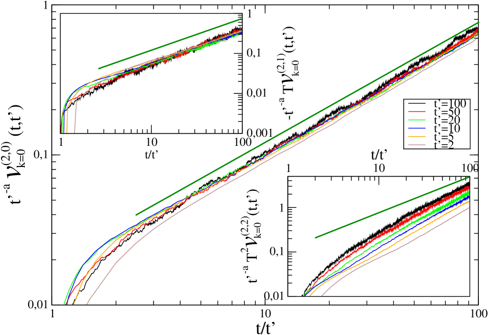
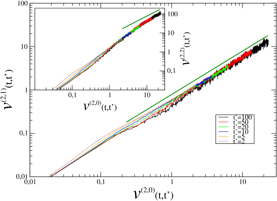
Figure 1: (Color online.) Clock model with $p=6$ heated from $T=0$ to $T=0.76$. Upper panel: The re-scaled moment $t^{\prime-a}{\cal V}_{k=0}^{(2,0)}(t,t^{\prime})$, with $a=0.76$, is plotted against $t/t^{\prime}$ in the main part of the figure, while the same plot for ${\cal V}_{k=0}^{(2,1)}$ (with a minus sign in order to have a positive quantity) and ${\cal V}_{k=0}^{(2,1)}$ is presented in the upper-left and lower-right insets, respectively. Different choices of $t^{\prime}$ correspond to different curves, see the key. The straight green bold line is the power law $(t/t^{\prime})^{0.8}$. Lower panel: Same data as in the upper panel but plotted in the parametric form $-{\cal V}_{k=0}^{(2,1)}(t,t^{\prime})$ against ${\cal V}_{k=0}^{(2,0)}(t,t^{\prime})$ (main part) and ${\cal V}_{k=0}^{(2,2)}(t,t^{\prime})$ against ${\cal V}_{k=0}^{(2,0)}(t,t^{\prime})$ (inset). The straight green bold line is the linear behavior (i.e. scaling functions are proportional).

Clock model with $p=12$

The results for $p=12$ are presented in Fig. 2. One observes the same qualitative behavior as in the case with $p=6$. With a value $a=0.83$ one obtains an excellent data collapse for ${\cal V}_{k=0}^{(2,0)}$ and ${\cal V}_{k=0}^{(2,1)}$, while for ${\cal V}_{k=0}^{(2,2)}$ the collapse is only asymptotically approached, similarly (but the collapse is somewhat better) to the case with $p=6$. Notice that this value of $a$ is basically the same as the one obtained for $p\to\infty$, where one has $a\simeq 0.83$ since $\eta\simeq 0.165$ and $z=2$ gupta . From $p=12$ onward, therefore, one does not expect to see any significant difference with the spin-wave analytic results. The scaling functions behave as $f^{(2,0)}(x)\sim f^{(2,1)}\sim x^{\alpha}$, with $\alpha=0.84$. For $f^{(2,2)}$ the data are consistent with an asymptotic convergence towards the same power-law behavior. This picture is confirmed by the parametric plots of $-{\cal V}_{k=0}^{(2,1)}$ and ${\cal V}_{k=0}^{(2,2)}$ against ${\cal V}_{k=0}^{(2,0)}$ presented in the lower panel of Fig. 2.

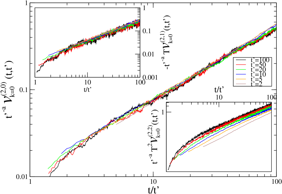
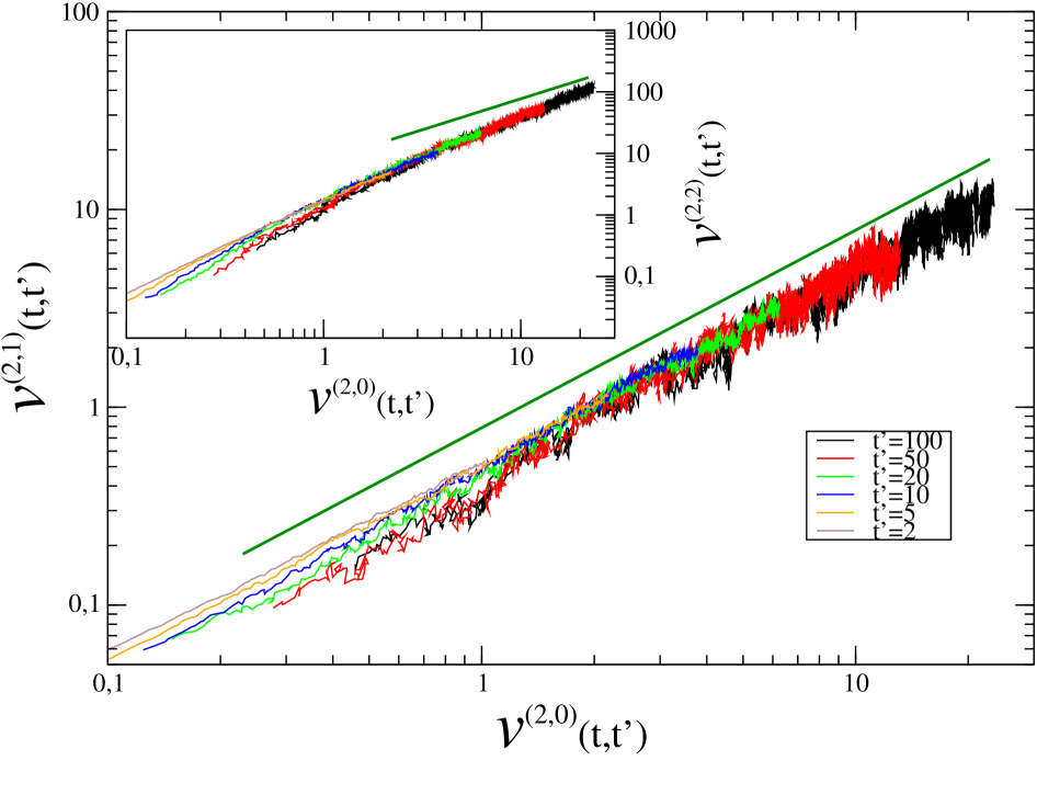
Figure 2: (Color online.) Clock model with $p=12$ heated from $T=0$ to $T=0.76$. Upper panel: The re-scaled moment $t^{\prime-a}{\cal V}_{k=0}^{(2,0)}(t,t^{\prime})$, with $a=0.83$, is plotted against $t/t^{\prime}$ in the main part of the figure, while the same plot for ${\cal V}_{k=0}^{(2,1)}$ (with a minus sign in order to have a positive quantity) and ${\cal V}_{k=0}^{(2,1)}$ is presented in the upper-left and lower-right insets, respectively. Different choices of $t^{\prime}$ correspond to different curves, see the key. Lower panel: Same data as in the upper panel but plotted in the parametric form $-{\cal V}_{k=0}^{(2,1)}(t,t^{\prime})$ against ${\cal V}_{k=0}^{(2,0)}(t,t^{\prime})$ (main part) and ${\cal V}_{k=0}^{(2,2)}(t,t^{\prime})$ against ${\cal V}_{k=0}^{(2,0)}(t,t^{\prime})$ (inset). The straight green bold line is the linear behavior (i.e. scaling functions are proportional).

V.2.2 Quench from infinite temperature

When quenching from $T_{i}\to\infty$ the presence of vortics makes the dynamics quite different from the one observed in the heating case vortici . It is therefore interesting to see how the scenario provided by the spin-wave approximation may or may not be modified in this case. In the following we present the results of simulations of the same system considered insofar, but with initial conditions extracted from an $T_{i}\to\infty$ equilibrium ensemble. We only discuss the case with $p=6$ since we found very similar results for $p=12$.

The second moments ${\cal V}_{k=0}^{(2,0)}(t,t^{\prime})$, ${\cal V}_{k=0}^{(2,1)}(t,t^{\prime})$ and ${\cal V}_{k=0}^{(2,2)}(t,t^{\prime})$ are plotted in Fig. 3. In this figure we used the same scaling procedure for the heated system, with the same exponent $a$ since, being an equilibrium quantity it should not depend upon the non-equilibrium protocol. As it is seen, this produces a quality of data collapse comparable to the case of the heated system. Strictly speaking, one should expect logarithmic correction to this scaling behavior, caused by the presence of vortices vortici . However, such corrections are very tiny in the asymptotic time domain and they cannot be detected from the inspection of our data. A major difference with respect to the heated system is, instead, the behavior of the scaling functions. Indeed, while $f^{(2,2)}$ keeps growing with the same power law of the heated system (the two quantities - in the heated and quenched case - are basically indistinguishable except for small $x$), $f^{(2,0)}$ and $f^{(2,1)}$ are changed to a much slower, logarithmic growth. From the parametric plots presented in the lower panel of Fig. 1 one argues that $f^{(2,0)}$ and $f^{(2,1)}$ are still asymptotically proportional. Interesting, in an intermediate time regime also $f^{(2,2)}$ grows proportionally to the other scaling functions. For larger times, however, there is a crossover to a faster growth. This interesting feature shows that ${\cal V}_{k=0}^{(2,2)}(t,t^{\prime})$ does not feel the presence of vortices, while the other moments do. Since these quantities have been proposed c4 ; noivarianze ; noichi2 ; Cocuyo as efficient tools to detect dynamical heterogeneities and to quantify cooperative lengths, our results suggest that different lengths are encoded in the different ${\cal V}$’s. A possible explanation could be that ${\cal V}_{k=0}^{(2,0)}$ and ${\cal V}_{k=0}^{(2,1)}$ detect the distance between vortices while ${\cal V}_{k=0}^{(2,2)}$ is only determined by the typical length of the smooth spin rotations (spin waves), but this subject should be further investigated. Notice also that the peculiar scaling of the ${\cal V}_{k=0}$’s found in the case of the quench has non-trivial consequences on the limiting behavior of the generalized FD ratios of Eq. (38). Indeed, since the ordinary FD ratio $X$ is finite noiteff , the disconnected terms subtracted off in Eq. (114) have the same scaling properties independently on $m$ and $m^{\prime}$. Hence the scaling of the ${\cal V}$’s directly inform us on the behavior of the composite operators ${\cal C}^{(n,m)}$ (37) and, in turn, of the ratios $X^{(n;m,m^{\prime})}$ of Eq. (38). Since the ${\cal V}$’s are found to scale with the same exponent $a$ but with a different form of the scaling function this implies that the limiting value $\lim_{t^{\prime}\to\infty}X^{(2;m,m^{\prime})}(t=yt^{\prime},t^{\prime})$ (with $y$ fixed) is finite. The same is true also when the limit $\lim_{t\to\infty}X^{(2;m,m^{\prime})}(t,t^{\prime})$ is taken (with $t^{\prime}$ sufficiently large) but only for $m\neq 2$ and $m^{\prime}\neq 2$. On the other hand, the same quantity is not finite for $m=2$ or $m^{\prime}=2$. This behavior is radically different from all the other cases studied insofar.

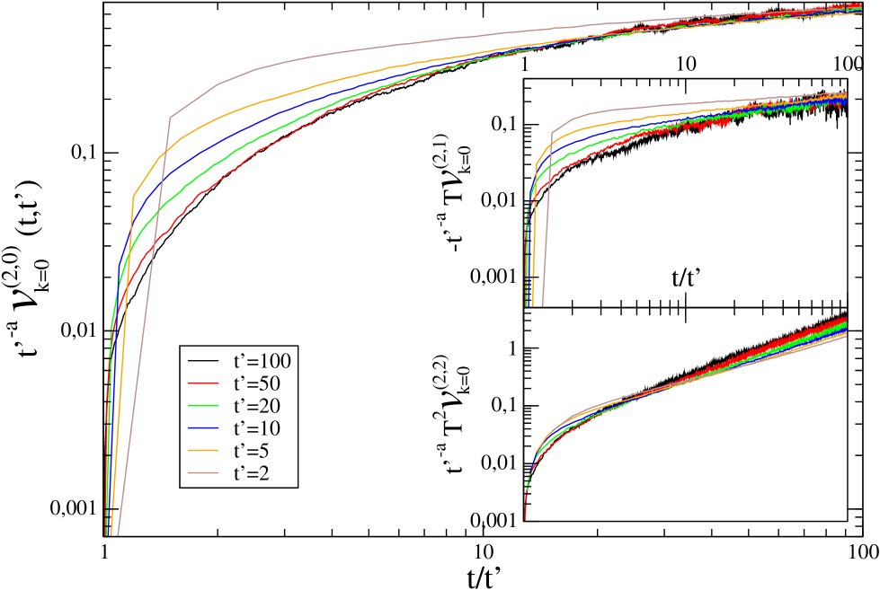
Figure 3: (Color online.) Upper panel: Clock model with $p=6$ quenched from $T=\infty$ to $T=0.76$. The re-scaled moment $t^{\prime-a}{\cal V}_{k=0}^{(2,0)}(t,t^{\prime})$, with $a=0.76$, is plotted against $t/t^{\prime}$ in the main part of the picture, while the same plot for ${\cal V}_{k=0}^{(2,1)}$ (with a minus sign in order to have a positive quantity) and ${\cal V}_{k=0}^{(2,1)}$ is presented in the upper and lower insets, respectively. Different choices of $t^{\prime}$ correspond to different curves, see key in the figure. Lower panel: Same data as in the upper panel but plotted in the parametric form $-{\cal V}_{k=0}^{(2,1)}(t,t^{\prime})$ against ${\cal V}_{k=0}^{(2,0)}(t,t^{\prime})$ (main part) and ${\cal V}_{k=0}^{(2,2)}(t,t^{\prime})$ against ${\cal V}_{k=0}^{(2,0)}(t,t^{\prime})$ (inset). The straight green bold line is the linear behavior (i.e. scaling functions are proportional).

VI Conclusions

In this paper we undertook the study of the out of equilibrium dynamics of some unfrustrated models with a finite FD ratio from the novel perspective of dynamic fluctuations. After defining in a proper way the fluctuating quantities the average of which yield the usual two-time correlation and linear response function, we evaluated the properties of their probability distribution and the scaling of the composite operators [defined in Eqs. (35) and (37)] made of products of $n$ of these fluctuating quantities. We showed that, in the model studied analytically, such composite fields in the asymptotic time domain scale in the same way when the total number $n$ of fluctuating parts involved is the same, irrespectively of how many factors are of the correlation or the linear response type. Therefore ratios between composite operators with the same $n$ converge to a finite value in the large time limit for any value of $n$. Since such composite operators are strictly related to higher order correlation and response functions, these ratios can be regarded as a generalization of the usual FD ratio above linear order. In the restricted context of the simple models considered analytically in this Article, their finite asymptotic value might speak about the significance of the notion of an effective temperature associated to the FD ratio. Indeed, for such a concept to be physically meaningful, one would ask such effective temperature to remain finite at any order. Related to that, the analytical results of this Article support the idea that fluctuations in aging systems are intimately related to the behavior of the FD ratio ChamonCugliandolo ; Cocuyo . The mechanism whereby a finite value of the generalized FD ratios is attained in the simple unfrustrated models considered analytically here might also be useful to understand the behavior of fluctuations in more realistic systems.

Besides, the analysis of this Article is also related to the problem of the detection of characteristic lengths form higher order correlations and response functions Cocuyo ; noichi2 ; lengths . One major problem in this context is which lengths are these higher order quantities sensitive to, and how. Interestingly enough, in all the models considered in this Article where a unique growing length is present the composite operators have the same asymptotic time-scaling (exponents and scaling functions). This indicates that the growing length enters different composite operators in the same scaling way. The different scaling functions found in the quenched clock model, where two different lengths are present, seems to indicate that different composite operators are sensitive to different lengths.

Some previous studies of the second-order momenta in different model systems had been performed and we wish now to confront our findings to these. In so doing, we will refine the picture of the dynamic scaling of fluctuations in i) coarsening systems quenched below their critical temperature; ii) disordered spin models such as the Edwards-Anderson spin-glass; iii) critical systems as the ones we studied here.

The results for the critical cases considered here (except possibly from the quenched clock model) are clearly different from what has been found in sub-critical quenches of simple coarsening systems noivarianze where the moments associated to the correlation scale differently from the ones where the fluctuations associated to the linear response enter. The analysis of the second-order momenta for a ferromagnet quenched to its critical point computed numerically in noivarianze and analytically in the spherical model in annibsollich unveil a behavior analogous to the one found in this paper and the scaling found by these authors conforms to the form given in Eq. (117). Monte Carlo simulations of the sub-critical dynamics of the $3d$ Edwards-Anderson spin-glass noispinglass suggest that the second moments in these glassy systems scale in the same way, in agreement with the conclusions arrived at in Chkecacu ; Cachcuke ; Cachcuigke ; Jaubert by analyzing the joint probability distribution of Sec. II.1. This claim has to be taken with the usual proviso that numerical simulations of glassy systems are hard to interpret beyond any doubt.

The analysis in this paper could be applied to other systems with glassy dynamics; thus helping to complete a general comprehension of fluctuations in problem with slow dynamics. Obvious candidates are kinetically constrained models kinetically-constrained , for which an analysis of out of equilibrium fluctuations along these lines was initiated in Chchcurese ; the one dimensional Glauber Ising model Garrahan , or random manifold problems, studied from an averaged perspective in Schehr among many other papers.

Appendix A Calculation of ${\cal C}_{\lambda}^{(n,0)}$

Using the exponential form of the cosine we have

$${\cal C}_{\lambda}^{(n,0)}=2^{-n}\langle\prod_{i=1}^{n}\left(e^{i\delta_{i,\lambda}}+e^{-i\delta_{i,\lambda}}\right)\rangle=2^{-n}\sum_{\{s_{i}=\pm 1\}}\langle e^{i\sum_{i=1,n}s_{i}\delta_{i,\lambda}}\rangle\;,$$ (118)

where $s_{i}=\pm 1$ are sign variables. Using the property $\langle\exp(\pm ia)\rangle=\exp(-\langle a^{2}\rangle/2)$, holding for any linear function $a(\xi)$ of $\xi$, since the $\delta_{i,\lambda}$ are themselves linear, one arrives at

$${\cal C}_{\lambda}^{(n,0)}=2^{-n}\sum_{\{s_{i}=\pm 1\}}e^{-\frac{1}{2}\langle\left(\sum_{i=1,n}s_{i}\delta_{i,\lambda}\right)^{2}\rangle}=2^{-n}\sum_{\{s_{i}=\pm 1\}}e^{-\frac{1}{2}\langle{\cal S}_{\lambda}^{2}\rangle}\;,$$ (119)

where the last equality defines the function ${\cal S}_{\lambda}$. We are now able to compute the $n$-times derivatives involved in Eq. (35). By taking them one at a time it is easy to check that $\partial_{\lambda_{1}}...\partial_{\lambda_{n}}e^{-\frac{1}{2}\langle{\cal S}_{\lambda}^{2}\rangle}=\left(\prod_{i=1}^{n}s_{i}\right)P^{(n)}({\cal S}_{\lambda},\{\partial\alpha_{\lambda_{i}}\})e^{-\frac{1}{2}\langle{\cal S}_{\lambda}^{2}\rangle}$, where the polynomial $P^{(n)}$ can be obtained by the recursive relation

$$P^{(r)}({\cal S}_{\lambda},\{\partial\alpha_{\lambda_{i}}\})=-P^{(r-1)}({\cal S}_{\lambda},\{\partial\alpha_{\lambda_{i}}\})\langle{\cal S}_{\lambda}\partial\alpha_{\lambda_{r}}\rangle+s_{r}^{-1}\partial_{\lambda_{r}}P^{(r-1)}({\cal S}_{\lambda},\{\partial\alpha_{\lambda_{i}}\})\;,$$ (120)

starting from $P^{(0)}({\cal S}_{\lambda},\{\partial\alpha_{\lambda_{i}}\})\equiv 1$. Hence one has

$$\partial{\cal C}^{(n,0)}_{\{\lambda\}=0}=2^{-n}\sum_{\{s_{i}=\pm 1\}}\left(\prod_{i=1}^{n}s_{i}\right)P^{(n)}({\cal S},\{\partial\alpha_{\lambda_{i}}\})e^{-\frac{1}{2}\langle{\cal S}^{2}\rangle}\;,$$ (121)

where ${\cal S}={\cal S}_{\{\lambda=0\}}$. The recursive equation (120) implies that $P^{(n)}$ is a sum which contains only products of correlators of the type

$$f=\langle{\cal S}\partial\alpha_{\lambda_{i}}\rangle\;,$$ (122)

and

$$\overline{f}=\langle\partial\alpha_{\lambda_{i}}\partial\alpha_{\lambda_{j}}\rangle\;.$$ (123)

Indeed, the first term in the rhs of the recursive equation (120) is itself a multiplication by a factor of type $f$, while the second term amounts to the replacement of some terms of type $f$ with others of type $\overline{f}$ (because $s_{j}^{-1}\partial_{\lambda_{j}}\langle{\cal S}\partial\alpha_{\lambda_{i}}\rangle=\langle\partial\alpha_{\lambda_{i}}\partial\alpha_{\lambda_{j}}\rangle$). It is easy to show (see App. B) that in a large time limit [for $t^{\prime}\to\infty$, with $y$ and $r$ (or $\zeta$) finite, or equivalently for $t-t^{\prime}\to\infty$ with $r$ (or $\zeta$) finite] the terms of type $\overline{f}$ are sub-dominant. Hence, in this time sector one has $P^{(n)}\simeq P^{(n)}(\{\langle{\cal S}\partial\alpha_{\lambda_{i}}\rangle\})$.

Appendix B Asymptotic analysis

Terms of kind $f$ are sums (over $i$) of contributions of the form

$$f(x_{i},x^{\prime}_{j};t_{i},t^{\prime}_{j})=\langle\phi(x_{i},t_{i})\partial_{t^{\prime}_{j}}\phi(x^{\prime}_{j},t^{\prime}_{j})\rangle=\partial_{t^{\prime}_{j}}C_{\phi}(|x_{i}-x^{\prime}_{j}|;t_{i},t^{\prime}_{j})\;,$$ (124)

for $j\leq m$, or

$$f(x_{i},x^{\prime}_{j};t_{i},t^{\prime}_{j})=\frac{1}{2T}\langle\phi(x_{i},t_{i})\xi(x^{\prime}_{j},t^{\prime}_{j})\rangle=R_{\phi}(|x_{i}-x^{\prime}_{j}|;t_{i},t^{\prime}_{j})$$ (125)

for $j>m$. Next to these there are analogous contributions that are obtained from the terms (124) and (125) with the replacement $(\vec{x}_{i},t_{i})\to(\vec{x}_{i}^{\prime},t_{i}^{\prime})$.

As it can be seen from the recursive equation (120), at the $r$-th step, terms of type $\overline{f}$ are generated from the quantities of type $f$ already present at step $r-1$ by replacing ${\cal S}$ with a $\partial\alpha_{\lambda_{r}}$. Then, in a generic term $\overline{f}$ it is always $i\neq j$. Using Eq. (96) for the quantities of type $\overline{f}$ with $i,j>m$, one has $\overline{f}(x^{\prime}_{i},x^{\prime}_{j};t^{\prime}_{i},t^{\prime}_{j})=(2T)^{-2}\langle\xi(x^{\prime}_{i},t^{\prime}_{i})\xi(x^{\prime}_{j},t^{\prime}_{j})\rangle$, which, restricting to the case, $(x^{\prime}_{i},t^{\prime}_{i})\neq(x^{\prime}_{j},t^{\prime}_{j})$ $\forall ij$, vanishes identically. On the other hand, for $i,j\leq m$, using Eq. (95) one has

$$\overline{f}(x^{\prime}_{i},x^{\prime}_{j};t^{\prime}_{i},t^{\prime}_{j})=\langle\partial_{t^{\prime}_{i}}\phi(x^{\prime}_{i},t^{\prime}_{i})\partial_{t^{\prime}_{j}}\phi(x^{\prime}_{j},t^{\prime}_{j})\rangle=\partial_{t^{\prime}_{i}}\partial_{t^{\prime}_{j}}C_{\phi}(r_{ij};t^{\prime}_{i},t^{\prime}_{j})\;,$$ (126)

and for $i\leq m$ and $j>m$

$$\overline{f}(x^{\prime}_{i},x^{\prime}_{j};t^{\prime}_{i},t^{\prime}_{j})=\frac{1}{2T}\langle\partial_{t^{\prime}_{i}}\phi(x^{\prime}_{i},t^{\prime}_{i})\xi(x^{\prime}_{j},t^{\prime}_{j})\rangle=\partial_{t^{\prime}_{i}}R_{\phi}(r_{ij};t^{\prime}_{i},t^{\prime}_{j})\;.$$ (127)

Comparing with the corresponding terms (124) and (125) of type $f$, there is an extra time derivative in the quantities $\overline{f}$. Using the scaling properties (53) and (54) one concludes that the latter are negligible in the large times domain [for $t^{\prime}\to\infty$, with $y$ and $r$ (or $\zeta$) finite, or equivalently for $t-t^{\prime}\to\infty$ with $r$ (or $\zeta$) finite].

Appendix C Scaling of $C_{\phi}(r;t,t^{\prime})$

From Eq. (50), for $2\Lambda^{2}(t-t^{\prime})\gg 1$ one can write

$$C_{\phi}(r;t,t^{\prime})=\frac{T}{4\pi}\int^{\zeta}_{\zeta\left[\frac{y-1}{y+1}\right]}dz\ \frac{e^{-z}}{z}$$ (128)

where $\zeta=r^{2}/[2(t-t^{\prime})]$ and $y=t/t^{\prime}$. For $\zeta\ll 1$, neglecting the exponential factor one obtains

$$C_{\phi}(r;t,t^{\prime})=\frac{T}{4\pi}\ln\left(\frac{y+1}{y-1}\right),$$ (129)

For larger values of $\zeta$, instead, letting $y\gg 1$ one finds

$$C_{\phi}(r;t,t^{\prime})=\frac{T}{2\pi}(y-1)^{-1}e^{-\zeta}.$$ (130)

Finally, we consider the equal times correlation. Proceeding as before we write

$$C_{\phi}(r;t,t)=\frac{T}{4\pi}\int^{\Lambda^{2}r^{2}}_{\frac{\Lambda^{2}r^{2}}{4\Lambda^{2}t+1}}dz\,\frac{e^{-z}}{z}\;.$$ (131)

For $\Lambda^{2}r^{2}\ll 1+4\Lambda^{2}t$, again neglecting the exponential, one has

$$C_{\phi}(r;t,t)=\frac{T}{4\pi}\ln(1+4\Lambda^{2}t)$$ (132)

For $1<\Lambda^{2}r^{2}<1+4\Lambda^{2}t$ one can split the integral as

$$C_{\phi}(r;t,t)=\frac{T}{4\pi}\left\{\int^{1}_{\frac{\Lambda^{2}r^{2}}{4\Lambda^{2}t+1}}\,\frac{e^{-z}}{z}\,+\,\int^{\Lambda^{2}r^{2}}_{1}\,\frac{e^{-z}}{z}\right\}\;,$$ (133)

and hence

$$C_{\phi}(r;t,t)\simeq\frac{T}{4\pi}\ln\left(\frac{1+4\Lambda^{2}t}{\Lambda^{2}r^{2}}\right)\;,$$ (134)

since the second integral in Eq. (133) is exponentially suppressed. Finally, for $\Lambda^{2}r^{2}\gg 1+4\Lambda^{2}t$, $C_{\phi}(r;t,t)$ is exponentially small. Putting everything together one has

$$C_{\phi}(r;t,t)\simeq\frac{T}{4\pi}\ln\left(\frac{1+4\Lambda^{2}t}{\Lambda^{2}r^{2}+1}\right)f_{cut}\left(\frac{\Lambda^{2}r^{2}}{1+4\Lambda^{2}t}\right)\;,$$ (135)

where $f_{cut}(z)$ is a cut-off function.

Acknowledgments L. F. C. wishes to thank Federico Romà and Daniel Domínguez for early discussions on this problem. This work was financially supported by ANR-BLAN-0346 (FAMOUS).

References

- (1) L. Bertini, A. De Sole, D. Gabrielli, G. Jona-Lasinio, and C. Landim, J. Stat. Phys. 107, 635 (2002); Phys. Rev. Lett. 87, 040601 (2001); J. Stat. Mech. P07014 (2007). T. Bodineau and B. Derrida, Phys. Rev. Lett. 92, 180601 (2004). J. Tailleur, J. Kurchan, and V. Lecomte, Phys. Rev. Lett. 99, 150602 (2007).
- (2) H. Touchette and R J. Harris, Large deviation approach to nonequilibrium systems, in R. Klages, W. Just, C. Jarzynski (eds), Nonequilibrium Statistical Physics of Small Systems: Fluctuation Relation and Beyond (Wiley-VCH, Weinheim, 2012).
- (3) D.J. Evans, E. G. D. Cohen, and G. P. Morris, Phys. Rev. Lett. 71, 2401 (1993). G. Gallavotti, and E.G.D. Cohen, J. Stat. Phys. 80, 931 (1995). For a recent review see also U. Seifert arXiv:1205.4176v1.
- (4) P. C. Hohenberg and B. I. Halperin, Rev. Mod. Phys. 49, 435 (1977).
- (5) A. J. Bray, Adv. Phys. 43, 357 (1994).
- (6) L. F. Cugliandolo, “Dynamics of glassy systems , in Slow Relaxation and non equilibrium dynamics in condensed matter, Les Houches Session 77 July 2002, J-L Barrat, J. Dalibard, J. Kurchan, M. V. Feigel man eds. (Springer-Verlag, 2003).
- (7) C. Chamon and L. F. Cugliandolo, J. Stat. Mech. P07022 (2007).
- (8) F. Corberi, L.F. Cugliandolo, and H. Yoshino, in Dynamical Heterogeneities in Glasses, Colloids, and Granular Media, L. Berthier, G. Biroli, J.-P. Bouchaud, L. Cipelletti and W. van Saarloos eds. (Oxford University Press, 2011).
- (9) E. Lippiello, F. Corberi, A. Sarracino, and M. Zannetti Phys. Rev. B 77, 212201 (2008); Phys. Rev. E 78, 041120 (2008).
- (10) A. Annibale and P. Sollich, J. Stat. Mech. P02064 (2009).
- (11) F. Corberi, E. Lippiello, A. Sarracino, and M. Zannetti, J. Stat. Mech. P04003 (2010).
- (12) C. Chamon, F. Corberi, L. F. Cugliandolo, J. Stat. Mech. P08015 (2011).
- (13) See the series of chapters in Dynamical Heterogeneities in Glasses, Colloids, and Granular Media, L. Berthier, G. Biroli, J.-P. Bouchaud, L. Cipelletti and W. van Saarloos eds. (Oxford University Press, 2011).
- (14) L. F. Cugliandolo, J. Kurchan, and G. Parisi, J. Phys. (France) 4, 1641 (1994).
- (15) G. Semerjian, L. F. Cugliandolo and A. Montanari, J. Stat. Phys. 115, 493 (2004).
- (16) L. F. Cugliandolo, J. Kurchan and L. Peliti, Phys. Rev. E 55, 3898 (1997).
- (17) A. Crisanti and F. Ritort, J. Phys. A 36, R181 (2003).
- (18) F. Corberi, E. Lippiello and M. Zannetti, J. Stat. Mech. P07002 (2007).
- (19) L. F. Cugliandolo, J. Phys. A 44, 483001 (2011).
- (20) T. H. Berlin, and M. Kac, Phys. Rev. 86, 821 (1952).
- (21) C. Chamon, L. F. Cugliandolo, H. Yoshino, J. Stat. Mech. (2006) P01006.
- (22) N. Pottier, Physica A 317, 371 (2003).
- (23) S. Bustingorry, J. L. Iguain, C. Chamon, L. F. Cugliandolo, and D. Domínguez, Europhys. Lett. 76, 856 (2006).
- (24) S. Bustingorry, L. F. Cugliandolo, J. L. Iguain, J. Stat. Mech. P09008 (2007).
- (25) J. L. Iguain, S. Bustingorry, A. B. Kolton, L. F. Cugliandolo, Phys. Rev. B 80, 094201 (2009).
- (26) Y-L. Chou and M. Pleimling, Physica A 391, 3585 (2012); J. Stat. Mech. P08007 (2010).
- (27) L. F. Cugliandolo, and J. Kurchan, Phys. Rev. Lett. 71, 173 (1993); J. Phys. A 27, 5749 (1994).
- (28) C. Godrèche and J.-M. Luck, J. Phys. A 33, 9141 (2000); J. Phys. Cond. Matter 14, 1589 (2002).
- (29) A. Crisanti and F. Ritort, Europhys. Lett. 66, 253 (2004); F. Ritort, J. Phys. Chem. B 108, 6893 (2004). F. Corberi, G. Gonnella, A. Piscitelli, and M. Zannetti, in press.
- (30) V. José, L. P. Kadanoff, S. Kirkpatrick, and D. R. Nelson, Phys. Rev. B 16, 1217 (1977); D. R. Nelson, in Phase Transitions and Critical Phenomena, Eds.: C. Domb and J. L. Lebowitz, (London, Academic Press, 1983).
- (31) J. M. Kosterlitz and D. J. Thouless, J. Phys. C 6, 1181 (1973); J. M. Kosterlitz, J. Phys. C 7, 1046 (1974).
- (32) M. S. S. Challa and D. P. Landau, Phys.Rev.B 33, 437 (1986); P. Czerner and U. Ritschel, Phys.Rev.E 53, 3333 (1996).
- (33) K. Kaski and J. D. Gunton, Phys. Rev.B 28, 5371 (1983). F. Liu and G. F. Mazenko, Phys. Rev.B 47, 2866 (1993). C. Chatelain, J. Stat. Mech P06006 (2004).
- (34) F. Corberi, E. Lippiello, and M. Zannetti, Phys. Rev. E 74, 041106 (2006).
- (35) A. D. Rutenberg and A. J. Bray, Phys. Rev. E 51, R1641 (1995).
- (36) J. M. Kosterlitz and D. J. Thouless, J. Phys. C 6, 1181 (1973).
- (37) L. Berthier, P. C. W. Holdsworth, M. Sellitto, J. Phys. A 34, 1805 (2001).
- (38) S. Abriet and D. Karevski, Eur. Phys. J B 37, 47 (2003).
- (39) X. W. Lei and B. Zheng, Phys. Rev. E 75, 040104(R) (2007)
- (40) C. Donati, S. C. Glotzer and P. Poole, Phys.Rev.Lett. 82, 5064 (1999); S. Franz, C. Donati, G. Parisi and S.C. Glotzer, Phil.Mag.B 79, 1827 (1999); S. Franz and G. Parisi, J.Phys.:Condens.Mat. 12, 6335 (2000); J.-P. Bouchaud and G. Biroli, Phys. Rev. B 72, 064204 (2005); C. Toninelli, M. Wyart, L. Berthier, G. Biroli and J.-P. Bouchaud, Phys.Rev.E 71, 041505 (2005); P. Mayer, H. Bissig, L. Berthier, L. Cipelletti, J.P. Garrahan, P. Sollich, and V. Trappe, Phys. Rev. Lett. 93, 115701 (2004).
- (41) E. Lippiello, F. Corberi, and M. Zannetti, Phys. Rev. E 71, 036104 (2005).
- (42) F. Corberi, E. Lippiello, and M. Zannetti Phys. Rev. E 72, 056103 (2005); Phys. Rev. E 72, 028103 (2005); J. Stat. Mech. P07002 (2007). E. Lippiello, F. Corberi, and M. Zannetti Phys. Rev. E 74, 041113 (2006). N. Andrenacci, F. Corberi, and E. Lippiello Phys. Rev. E 73, 046124 (2006); Phys. Rev. E 74 (2006). R. Burioni, D. Cassi, F. Corberi, and A. Vezzani Phys. Rev. Lett. 96, 235701 (2006); Phys. Rev. E 75, 011113 (2007). F. Corberi, A. Gambassi, E. Lippiello, and M. Zannetti J. Stat. Mech. P02013 (2008). F. Corberi, and L.F. Cugliandolo J. Stat. Mech. P05010 (2009); J. Stat. Mech. P09015 (2009). F. Corberi, E. Lippiello, A. Sarracino, and M. Zannetti Phys. Rev. E 81, 011124 (2010). F.Corberi, E.Lippiello, A.Mukherjee, S.Puri, and M.Zannetti J. Stat. Mech. P03016 (2011). R. Burioni, F. Corberi, and A. Vezzani, J. Stat. Mech. P12024 (2010).
- (43) R. Gupta and C. F. Baillie, Phys. Rev. B 45, 2883 (1992).
- (44) B. Yurke, A. N. Pargellis, T. Kovacs and D. A. Huse, Phys. Rev. E 47, 1525 (1993). F. Rojas and A. D. Rutenberg, Phys. Rev. E 60, 212 (1999). A. J. Bray, A. J. Briant and D. K. Jervis, Phys. Rev. Lett. 84, 1503 (2000). A. J. Bray, Phys. Rev. E 62, 103 (2000). A. Jelić and L. F. Cugliandolo, J. Stat. Mech. P02032 (2011).
- (45) F. Corberi, E. Lippiello, and M. Zannetti, J. Stat. Mech. P12007 (2004).
- (46) C. Chamon, M. P. Kennett, H. E. Castillo, L. F. Cugliandolo, Phys. Rev. Lett. 89, 217201 (2002). H. E. Castillo, Phys. Rev. B 78, 214430 (2008). G. A. Mavimbela and H. E. Castillo, Time reparametrization invariance in arbitrary range p-spin models: symmetric versus non-symmetric dynamics, arXiv:1011.2225.
- (47) H. E. Castillo, C. Chamon, L. F. Cugliandolo, M. P. Kennett, Phys. Rev. Lett. 88, 237201 (2002).
- (48) H. E. Castillo, C. Chamon, L. F. Cugliandolo, J. L. Iguain, and M. P. Kennett, Phys. Rev. B 68, 134442 (2003).
- (49) L. D. C. Jaubert, C. Chamon, L. F. Cugliandolo, and M. Picco, J. Stat. Mech. P05001 (2007).
- (50) D. A. Huse, J. Appl. Phys. 64, 5776 (1988). C. Donati, S. C. Glotzer and P. Poole, Phys. Rev. Lett. 82, 5064 (1999). S. Franz, C. Donati, G. Parisi and S. C. Glotzer, Phil. Mag. B 79, 1827 (1999). S. Franz and G. Parisi, J. Phys.: Condens. Mat. 12, 6335 (2000). C. Toninelli, M. Wyart, L. Berthier, G. Biroli and J.P. Bouchaud, Phys. Rev. E 71, 041505 (2005). P. Mayer, H. Bissig, L. Berthier, L. Cipelletti, J.P. Garrahan, P. Sollich, and V. Trappe, Phys. Rev. Lett. 93, 115701 (2004). J.P.Bouchaud and G.Biroli, Phys.Rev.B 72, 064204 (2005). L. Berthier, G. Biroli, J.P. Bouchaud, L.Cipelletti, D. El Masri, D. L H ote,F. Ladieu and M. Pierno, Science 310, 1797 (2005).
- (51) S. Leonard, P. Mayer, P. Sollich, L. Berthier, and J. P. Garrahan J. Stat. Mech. P07017 (2007). J. P. Garrahan, P. Sollich, and C. Toninelli “Kinetically Constrained Models” in Dynamical heterogeneities in glasses, colloids, and granular media, L. Berthier, G. Biroli, J-P Bouchaud, L. Cipelletti and W. van Saarloos eds. (Oxford University, 2011).
- (52) C. Chamon, P. Charbonneau, L. F. Cugliandolo, D. Reichman, M. Sellitto, J. Chem. Phys. 121, 10120 (2004).
- (53) P. Mayer and P. Sollich, J. Phys. A 37, 9 (2004). P. Mayer, P. Sollich, L. Berthier, and J. P. Garrahan J. Stat. Mech. P05002 (2005).
- (54) G. Schehr and P. Le Doussal, Phys. Rev. Lett. 93, 217201 (2004).