Triakis Solids and Harmonic Functions

Abstract

We describe the harmonic functions for certain isohedral triakis solids. They are the first examples for which polyhedral harmonics is strictly larger than group harmonics.
Keywords: polyhedral harmonics; group harmonics; isohedral triakis tetrahedron; isohedral triakis octahedron; finite reflection groups; invariant differential equations.

1 Introduction

A harmonic function on $\mathbb{R}^{n}$ is a distribution solution to the Laplace equation

$$\varDelta f=(\partial_{1}^{2}+\cdots+\partial_{n}^{2})f=0,\qquad\partial_{i}=\partial/\partial x_{i},$$ (1)

which is necessarily a smooth function. A classical theorem of Gauss and Koebe states that a continuous function on $\mathbb{R}^{n}$ is harmonic if and only if it satisfies the mean value property with respect to the sphere $S^{n-1}$. On the other hand the Laplacian $\varDelta$ admits an invariant-theoretic interpretation relative to the orthogonal group $O(n)$. Namely the $\mathbb{R}$-algebra of $O(n)$-invariant polynomials in $x=(x_{1},\dots,x_{n})$ is generated by the squared distance function $\varphi(x)=x_{1}^{2}+\cdots+x_{n}^{2}$ and the Laplacian $\varDelta=\varphi(\partial)$ is the result of substituting $\partial=(\partial_{1},\dots,\partial_{n})$ into $\varphi(x)$. These two characterizations of harmonic functions allow us to generalize the notion in two directions, that is, to polyhedral harmonics and to group harmonics.

Let $P$ be an $n$-dimensional polytope in $\mathbb{R}^{n}$ and $P(k)$ the $k$-dimensional skeleton of $P$, that is, the union of all $k$-dimensional faces of $P$. A continuous function $f(x)$ on $\mathbb{R}^{n}$ is said to be $P(k)$-harmonic if it satisfies the mean value property with respect to $P(k)$, that is, if

$$f(x)=\dfrac{1}{|P(k)|}\int_{P(k)}f(x+ry)\,d\mu_{k}(y)\qquad(\,{}^{\forall}x\in\mathbb{R}^{n},\,{}^{\forall}r>0),$$

where $\mu_{k}$ is the $k$-dimensional Euclidean measure on $P(k)$ with $|P(k)|:=\mu_{k}(P(k))$ being its total volume. Let $\mathcal{H}_{P(k)}$ denote the set of all $P(k)$-harmonic functions on $\mathbb{R}^{n}$. A general result of Iwasaki [5, Theorem 1.1] states that $\mathcal{H}_{P(k)}$ is a finite-dimensional linear space of polynomials. It is naturally an $\mathbb{R}[\partial]$-module, that is, stable under partial differentiations. If $G(k)$ is the symmetry group of $P(k)$, then it is also an $\mathbb{R}[G(k)]$-module, that is, stable under the natural action of $G(k)$. Moreover, if $P(k)$ enjoys ample symmetry, that is, if $G(k)$ acts on $\mathbb{R}^{n}$ irreducibly then $\mathcal{H}_{P(k)}$ is a finite-dimensional linear space of harmonic polynomials [5, Theorem 2.4].

Let $G$ be a subgroup of $O(n)$ and $\mathbb{R}[x]^{G}$ the $\mathbb{R}$-algebra of $G$-invariant polynomials of $x=(x_{1},\dots,x_{n})$. A $G$-harmonic function on $\mathbb{R}^{n}$ is a distribution solution to the system of PDEs:

$$\varphi(\partial)f=0\qquad(\,{}^{\forall}\varphi(x)\in\mathbb{R}[x]^{G}_{+}),$$ (2)

where $\mathbb{R}[x]^{G}_{+}$ is the maximal ideal of $\mathbb{R}[x]^{G}$ consisting of those $\varphi(x)$’s without constant term: $\varphi(0)=0$ (see Helgason [4, Chap. I​I​I]). Let $\mathcal{H}_{G}$ denote the set of all $G$-harmonic functions on $\mathbb{R}^{n}$. To define system (2), the polynomial $\varphi(x)$ may not range over all $\mathbb{R}[x]^{G}_{+}$, but only over a set of generators of $\mathbb{R}[x]^{G}_{+}$. For example, if $G$ is the entire $O(n)$ then $\mathbb{R}[x]^{O(n)}_{+}$ is generated by the squared distance function only, so that system (2) reduces to the single Laplace equation (1). In this article, $G$ will be a finite group in general and a finite reflection group in particular. Steinberg [9] shows that if $G$ is a finite group then $\mathcal{H}_{G}$ is a finite-dimensional linear space of polynomials with $\dim\mathcal{H}_{G}\geq|G|$, the order of $G$. When $G$ is a finite reflection group, he goes on to determine $\mathcal{H}_{G}$ explicitly. Namely, as an $\mathbb{R}[\partial]$-module $\mathcal{H}_{G}$ is generated by the fundamental alternating polynomial $\varDelta_{G}(x)$ of $G$, and as an $\mathbb{R}[G]$-module it is the regular representation of $G$, in particular $\dim\mathcal{H}_{G}=|G|$.

When $G=G(k)$ is the symmetry group of $P(k)$, it makes sense to compare $\mathcal{H}_{P(k)}$ with $\mathcal{H}_{G(k)}$. According to a result in [5, formula (2.14)] there is always the inclusion

$$\mathcal{H}_{G(k)}\subset\mathcal{H}_{P(k)}\qquad(k=0,\dots,n).$$ (3)

It is known that $\mathcal{H}_{P(k)}$ coincides with $\mathcal{H}_{G(k)}$ when $P$ is any regular convex polytope with center at the origin, in which case $G(k)$ is an irreducible finite reflection group so that $\mathcal{H}_{P(k)}=\mathcal{H}_{G(k)}$ is determined by Steinberg’s theorem; see Iwasaki [6, Theorem 4.4] and the references therein. One can show that the coincidence also occurs, for example, for the truncated icosahedron $[5,6,6]$ of an Archimedean solid, or the soccer ball. So far, however, no polytope with ample symmetry has been known for which inclusion (3) is strict (for some $k>0$), that is, polyhedral harmonics is strictly larger than group harmonics. The aim of this article is to present the first examples of such polytopes. They arise from a one-parameter family of isohedral triakis tetrahedra as well as from a one-parameter family of isohedral triakis octahedra in three dimensions. The former family contains a desired example for $k=1$, but none for $k=0,2,3$ (see Theorem 2.1), while the latter family contains such an example for every $k=0,1,2,3$ (see Theorem 5.1). In this respect the latter family is more interesting than the former, but in any case we begin with the simpler case of the former family and then proceed to the latter.

2 A Family of Isohedral Triakis Tetrahedra

Figure 1: Adjoining a pyramid to a face of a regular tetrahedron; $\overline{\mathrm{O}\mathrm{d}}:\overline{\mathrm{O}\mathrm{d}^{\prime}}=r:1$.

An isohedral triakis tetrahedron is obtained from a regular tetrahedron by adjoining to each face of it a pyramid (based on that face) of appropriate height, or excavating such a pyramid, where a polyhedron is said to be isohedral if its symmetry group is transitive on its faces, that is, if all faces are equivalent under symmetries of the polyhedron; see Grünbaum and Shephard [3]. Our triakis tetrahedron $P$ depends on a positive parameter $r$. To describe it more neatly, let $T$ be the regular tetrahedron with which we get started; it is centered at the origin $\mathrm{O}$ and with four vertices $\mathrm{A}$, $\mathrm{B}$, $\mathrm{C}$, $\mathrm{D}$. If $\mathrm{d}^{\prime}$ denotes the center of the face $\mathrm{A}\mathrm{B}\mathrm{C}$, then the pyramid based on this face has the top vertex $\mathrm{d}$ that lies on the ray emanating from $\mathrm{O}$ and passing through $\mathrm{d}^{\prime}$ in such a manner that the distance ratio $\overline{\mathrm{O}\mathrm{d}}:\overline{\mathrm{O}\mathrm{d}^{\prime}}$ is $r:1$ (see Figure 1). The polyhedron $P$ has four six-valent vertices $\mathrm{A}$, $\mathrm{B}$, $\mathrm{C}$, $\mathrm{D}$ and four three-valent vertices $\mathrm{a}$, $\mathrm{b}$, $\mathrm{c}$, $\mathrm{d}$, where $\mathrm{a}$, $\mathrm{b}$, $\mathrm{c}$ are defined in a similar manner as the vertex $\mathrm{d}$ is, and $P$ has twelve faces and eighteen edges.

Let us look more closely at the polyhedron $P$ for various values of $r$ (see Figure 2).

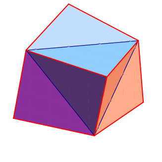
$r>3$

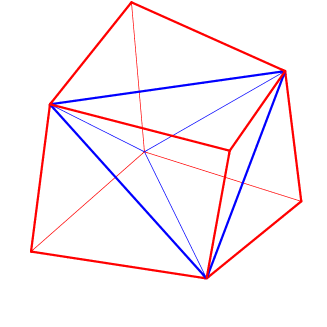
$r>3$

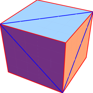
$r=3$

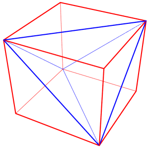
$r=3$

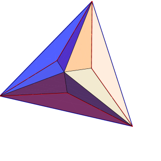
$0<r<1$

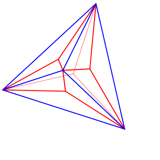
$0<r<1$

Figure 2: A one-parameter family of isohedral triakis tetrahedra. Each polyhedron is shown in a “cardboard” view on the left, as well as in a skeletal view on the right. Polyhedron with $1<r<3$ is not indicated, but imaginable from the one with $r>3$, although the former is convex while the latter is not. See also a series of pictures in Grünbaum [2, Fig. 14].

The values $r=1$ and $r=3$ are special in that as a point set, $P$ degenerates to the tetrahedron $T$ at $r=1$ and it becomes a cube $C$ at $r=3$. For $r>1$, $P$ is obtained from $T$ by adjoining a pyramid to each face of $T$, while for $0<r<1$, it is obtained by excavating such a pyramid. Moreover $P$ is convex if and only if $1\leq r\leq 3$, in which interval the value $r=9/5$ is distinguished in that $P$ becomes a Catalan solid [1, 7], or an Archimedean dual solid, whose dual is the truncated tetrahedron $[3,6,6]$. When $r=1$, although the four points $\mathrm{A}$, $\mathrm{B}$, $\mathrm{C}$, $\mathrm{d}$ are coplanar, we think of $\mathrm{A}\mathrm{B}\mathrm{d}$, $\mathrm{B}\mathrm{C}\mathrm{d}$, $\mathrm{A}\mathrm{C}\mathrm{d}$ as distinct faces of $P$, and thus $\mathrm{A}\mathrm{d}$, $\mathrm{B}\mathrm{d}$, $\mathrm{C}\mathrm{d}$ as edges, and $\mathrm{d}$ as a vertex of $P$. Similarly, when $r=3$, although the four points $\mathrm{A}$, $\mathrm{B}$, $\mathrm{c}$, $\mathrm{d}$ are coplanar, we think of $\mathrm{A}\mathrm{B}\mathrm{c}$ and $\mathrm{A}\mathrm{B}\mathrm{d}$ as distinct faces of $P$, and thus $\mathrm{A}\mathrm{B}$ as an edge of $P$. With this convention, as a combinatorial polyhedron, $P$ has the constant skeletal structure for all $r>0$.

Let $G(k)$ be the symmetry group of $P(k)$. When $k=1$, for every $r>0$ the group $G(k)$ is always the same as the symmetry group of the tetrahedron $T$, which we denote by $W(\mathrm{A}_{3})$ since it is a Weyl group of type $\mathrm{A}_{3}$. On the other hand, when $k=0,2,3$, the group $G(k)$ stays the same as $W(\mathrm{A}_{3})$ as long as $r\neq 3$, but at $r=3$ it jumps up to be the symmetry group of the cube $C$, which is denoted by $W(\mathrm{B}_{3})$ as being a Weyl group of type $\mathrm{B}_{3}$. For simplicity of notation, $\mathcal{H}_{W(\mathrm{A}_{3})}$ and $\mathcal{H}_{W(\mathrm{B}_{3})}$ are abbreviated to $\mathcal{H}_{\mathrm{A}_{3}}$ and $\mathcal{H}_{\mathrm{B}_{3}}$ respectively. Note that

$$\mathcal{H}_{\mathrm{A}_{3}}\varsubsetneq\mathcal{H}_{\mathrm{B}_{3}},\qquad\dim\mathcal{H}_{\mathrm{A}_{3}}=24,\qquad\dim\mathcal{H}_{\mathrm{B}_{3}}=48.$$

It is our problem to consider how $\mathcal{H}_{P(k)}$ behaves as $r$ varies and when $\mathcal{H}_{P(k)}$ is strictly larger than $\mathcal{H}_{G(k)}$. Any value of $r$ with this phenomenon is referred to as a critical value. It turns out that the vertex $(k=0)$ and face $(k=2)$ problems have no critical values, but the edge $(k=1)$ problem certainly has a critical value $r_{1}=3.62398\cdots$. It is an algebraic integer of degree six that is the unique positive root of a sextic equation

$$\chi_{1}(r):=r^{6}+2r^{5}+r^{4}-36r^{3}-45r^{2}-270r-405=0.$$ (4)

How this algebraic equations arises will be explained in §4.2. The volume problem $(k=3)$ need not be dealt with independently, since the isohedrality of $P$ implies $\mathcal{H}_{P(2)}=\mathcal{H}_{P(3)}$ by a result of [5, Theorem 2.2] so that the face and volume problems have the same solution.

Theorem 2.1

For the family of isohedral triakis tetrahedra, $\mathcal{H}_{P(k)}$ is strictly larger than $\mathcal{H}_{G(k)}$ if and only if $k=1$ and $r=r_{1}=3.62398\cdots$. The function space $\mathcal{H}_{P(k)}$ is given by

$$\mathcal{H}_{P(k)}=\begin{cases}\mathcal{H}_{\mathrm{B}_{3}}&(\mbox{if either $k=1$, $r=r_{1};$ or $k=0,2,3$, $r=3$}),\\ \mathcal{H}_{\mathrm{A}_{3}}&(\mbox{otherwise}).\end{cases}$$ (5)

This theorem asserts that when $k=1$ and $r$ is at the critical value $r_{1}$, the figure $P(1)$ has only the same symmetries as a tetrahedron, but $\mathcal{H}_{P(1)}$ jumps up to become the space of cubic harmonics, which is strictly larger than that of tetrahedral harmonics. For each $k=0,2,3$, a jumping phenomenon also occurs at $r=3$ with the space $\mathcal{H}_{P(k)}$ jumping from $\mathcal{H}_{\mathrm{A}_{3}}$ to $\mathcal{H}_{\mathrm{B}_{3}}$, but at the same time the group $G(k)$ also jumps from $W(\mathrm{A}_{3})$ to $W(\mathrm{B}_{3})$. Altogether, the equality $\mathcal{H}_{P(k)}=\mathcal{H}_{G(k)}$ continues to hold and no critical phenomenon occurs at $r=3$. After a review in §3 on PDEs that characterize polyhedral harmonics, Theorem 2.1 will be established in §4.

3 Invariant Differential Equations

Iwasaki [5, Theorem 2.1] derives a system of partial differential equations

$$\tau_{m}^{(k)}(\partial)f=0\qquad(m=1,2,3,\dots)$$ (6)

that characterizes $\mathcal{H}_{P(k)}$ as its distribution solution space. Here is a brief review of it when $P$ is a three-dimensional polyhedron and $k=0,1,2$. For $j=0,1,2$, let $\{P_{i_{j}}\}_{i_{j}\in I_{j}}$ be the set of all $j$-dimensional faces of $P$, where $I_{j}$ is an index set. Let $H_{i_{j}}$ be the $j$-dimensional affine subspace of $\mathbb{R}^{3}$ containing $P_{i_{j}}$. Let $p_{i_{j}}$ be the foot of orthogonal projection from the origin $\mathrm{O}$ down to $H_{i_{j}}$. We mean by $i_{j}\prec i_{j+1}$ that $P_{i_{j}}$ is a face of $P_{i_{j+1}}$. If $i_{j}\prec i_{i_{j+1}}$ then the vector $p_{i_{j}}-p_{i_{j+1}}$ is parallel to the outer unit normal vector $\mbox{\boldmath$n$}_{i_{j},i_{j+1}}$ of $\partial P_{i_{j+1}}$ in $H_{i_{j+1}}$ at the face $P_{i_{j}}$, so that a number $[i_{j}:i_{j+1}]$, called the incidence number, is defined by the relation $p_{i_{j}}-p_{i_{j+1}}=[i_{j}:i_{j+1}]\mbox{\boldmath$n$}_{i_{j},i_{j+1}}$. Put $I(1)=\{i=(i_{0},i_{1})\,:\,i_{0}\prec i_{1}\}$, $I(2)=\{i=(i_{0},i_{1},i_{2})\,:\,i_{0}\prec i_{1}\prec i_{2}\}$, and define

$$[i]=\begin{cases}[i_{0}:i_{1}]&(i=(i_{0},i_{1})\in I(1)),\\ [i_{0}:i_{1}][i_{1}:i_{2}]&(i=(i_{0},i_{1},i_{2})\in I(2)).\end{cases}$$

Then $\tau_{m}^{(k)}(x)$, $k=0,1,2$, are homogeneous polynomials of degree $m$ defined by

$$\tau_{m}^{(0)}(x) :=\sum_{i_{0}\in I_{0}}\langle p_{i_{0}},x\rangle^{m},$$ (7)

$$\tau_{m}^{(1)}(x) :=\sum_{i\in I(1)}[i]\,h_{m}(\langle p_{i_{0}},x\rangle,\,\langle p_{i_{1}},x\rangle),$$ (8)

$$\tau_{m}^{(2)}(x) :=\sum_{i\in I(2)}[i]\,h_{m}(\langle p_{i_{0}},x\rangle,\,\langle p_{i_{1}},x\rangle,\,\langle p_{i_{2}},x\rangle),$$ (9)

where $\langle\,\cdot\,,\,\cdot\,\rangle$ is the standard inner product on $\mathbb{R}^{3}$ and $h_{m}$ stands for the complete symmetric polynomial of degree $m$ in two or three variables (see e.g. Macdonald [8]).

The general construction mentioned above will be applied to the particular case of our polyhedron $P$ upon adjusting the notation to the current situation. In order to represent the index sets $I_{0}$, $I_{1}$, $I_{2}$, it would be best to let the vertices, edges and faces to speak of themselves:

$$I_{0} =\{\mathrm{A},\mathrm{B},\mathrm{C},\mathrm{D}\}\cup\{\mathrm{a},\mathrm{b},\mathrm{c},\mathrm{d}\},$$

$$I_{1} =\{\mathrm{A}\mathrm{B},\mathrm{A}\mathrm{C},\mathrm{A}\mathrm{D},\mathrm{B}\mathrm{C},\mathrm{B}\mathrm{D},\mathrm{C}\mathrm{D}\}\cup\{\mathrm{A}\mathrm{b},\mathrm{A}\mathrm{c},\mathrm{A}\mathrm{d},\mathrm{B}\mathrm{a},\mathrm{B}\mathrm{c},\mathrm{B}\mathrm{d},\mathrm{C}\mathrm{a},\mathrm{C}\mathrm{b},\mathrm{C}\mathrm{d},\mathrm{D}\mathrm{a},\mathrm{D}\mathrm{b},\mathrm{D}\mathrm{c}\},$$

$$I_{2} =\{\mathrm{A}\mathrm{B}\mathrm{c},\mathrm{A}\mathrm{B}\mathrm{d},\mathrm{A}\mathrm{C}\mathrm{b},\mathrm{A}\mathrm{C}\mathrm{d},\mathrm{A}\mathrm{D}\mathrm{b},\mathrm{A}\mathrm{D}\mathrm{c},\mathrm{B}\mathrm{C}\mathrm{a},\mathrm{B}\mathrm{C}\mathrm{d},\mathrm{B}\mathrm{D}\mathrm{a},\mathrm{B}\mathrm{D}\mathrm{c},\mathrm{C}\mathrm{D}\mathrm{a},\mathrm{C}\mathrm{D}\mathrm{b}\},$$

where $\{\cdots\}$ stands for an orbit under symmetries. For an index $\mathrm{A}\mathrm{d}\in I_{1}$, the same symbol $\mathrm{A}\mathrm{d}$ denotes the foot of orthogonal projection from the origin $\mathrm{O}$ to the affine line $\ell_{\mathrm{A}\mathrm{d}}$ passing through $\mathrm{A}$ and $\mathrm{d}$; this rule also applies to another index $\mathrm{A}\mathrm{B}\in I_{1}$ as well as to all the other indices of $I_{1}$. In a similar manner, for an index $\mathrm{A}\mathrm{B}\mathrm{d}\in I_{2}$, the same symbol $\mathrm{A}\mathrm{B}\mathrm{d}$ denotes the foot of orthogonal projection from $\mathrm{O}$ to the affine plane $H_{\mathrm{A}\mathrm{B}\mathrm{d}}$ passing through $\mathrm{A}$, $\mathrm{B}$, $\mathrm{d}$, with this rule applying to all the other indices of $I_{2}$; see Figure 3.

Figure 3: Combinatorial data for the system (6) of PDEs.

Up to symmetries there are three types of vertex-to-edge incidence relations:

$$(\mathrm{VE}1)\quad\mathrm{A}\prec\mathrm{A}\mathrm{B},\qquad(\mathrm{VE}2)\quad\mathrm{A}\prec\mathrm{A}\mathrm{d},\qquad(\mathrm{VE}3)\quad\mathrm{d}\prec\mathrm{A}\mathrm{d}.$$ (10)

On the other hand, up to symmetries there are two types of edge-to-face incidence relations:

$$(\mathrm{EF}1)\quad\mathrm{A}\mathrm{B}\prec\mathrm{A}\mathrm{B}\mathrm{d},\qquad(\mathrm{EF}2)\quad\mathrm{A}\mathrm{d}\prec\mathrm{A}\mathrm{B}\mathrm{d}.$$ (11)

The incidence number of an incidence relation depends only on its type. Let $\mathrm{ve}_{\nu}$ denote the incidence number of type ($\mathrm{VE}\nu$), $\nu=1,2,3$, and $\mathrm{ef}_{\nu}$ denote that of type ($\mathrm{EF}\nu$), $\nu=1,2$. For example we have $[\mathrm{A}:\mathrm{A}\mathrm{d}]=\mathrm{ve}_{2}$ and $[\mathrm{A}\mathrm{d}:\mathrm{A}\mathrm{B}\mathrm{d}]=\mathrm{ef}_{2}$, so that $\mathrm{A}-\mathrm{A}\mathrm{d}=\mathrm{ve}_{2}\,\mbox{\boldmath$n$}_{\mathrm{A},\mathrm{A}\mathrm{d}}$ and $\mathrm{A}\mathrm{d}-\mathrm{A}\mathrm{B}\mathrm{d}=\mathrm{ef}_{2}\,\mbox{\boldmath$n$}_{\mathrm{A}\mathrm{d},\mathrm{A}\mathrm{B}\mathrm{d}}$ for $\mathrm{A}\prec\mathrm{A}\mathrm{d}\prec\mathrm{A}\mathrm{B}\mathrm{d}$. These numbers are positive in the situation of Figure 3, but they or some other incidence numbers may be negative for some values of $r$.

For explicit calculations, it is convenient to work with Cartesian coordinates by putting

$$\mathrm{A}=(1,-1,-1),\quad\mathrm{B}=(-1,1,-1),\quad\mathrm{C}=(-1,-1,1),\quad\mathrm{D}=(1,1,1).$$ (12)

The symmetry group $W(\mathrm{A}_{3})$ of the tetrahedron $T$ then admits an invariant basis

$$e_{2}(x):=x_{1}^{2}+x_{2}^{2}+x_{3}^{2},\quad e_{3}(x):=x_{1}x_{2}x_{3},\quad e_{4}(x):=x_{2}^{2}x_{3}^{2}+x_{3}^{2}x_{1}^{2}+x_{1}^{2}x_{2}^{2},$$

so that $\mathcal{H}_{\mathrm{A}_{3}}$ can be characterized as the solution space to the system of PDEs:

$$e_{2}(\partial)f=e_{3}(\partial)f=e_{4}(\partial)f=0.$$ (13)

As an $\mathbb{R}[\partial]$-module, $\mathcal{H}_{\mathrm{A}_{3}}$ is generated by the fundamental alternating polynomial

$$\varDelta_{\mathrm{A}_{3}}(x)=(x_{1}^{2}-x_{2}^{2})(x_{2}^{2}-x_{3}^{2})(x_{3}^{2}-x_{1}^{2}).$$

If the vertices of $T$ are taken as in formula (12), then $C$ is the cube with vertices at $(\pm 1,\pm 1,\pm 1)$. The symmetry group $W(\mathrm{B}_{3})$ of $C$ then admits an invariant basis $e_{2}(x)$, $e_{4}(x)$, $e_{6}(x):=e_{3}^{2}(x)$, so that $\mathcal{H}_{\mathrm{B}_{3}}$ can be characterized as the solution space to the system of PDEs:

$$e_{2}(\partial)f=e_{4}(\partial)f=e_{6}(\partial)f=0.$$ (14)

As an $\mathbb{R}[\partial]$-module, $\mathcal{H}_{\mathrm{B}_{3}}$ is generated by the fundamental alternating polynomial

$$\varDelta_{\mathrm{B}_{3}}(x)=x_{1}x_{2}x_{3}(x_{1}^{2}-x_{2}^{2})(x_{2}^{2}-x_{3}^{2})(x_{3}^{2}-x_{1}^{2}).$$ (15)

Since $P$ is at least $W(\mathrm{A}_{3})$-symmetric, $\tau_{m}^{(k)}(x)$ must be $W(\mathrm{A}_{3})$-invariant and hence can be written in unique ways as polynomials of $e_{2}(x)$, $e_{3}(x)$, $e_{4}(x)$. For $m=1,\dots,6$, one can write

$$\tau_{1}^{(k)}(x) =0, \tau_{2}^{(k)}(x) =a_{2}^{(k)}\,e_{2}(x),$$

$$\tau_{3}^{(k)}(x) =a_{3}^{(k)}\,e_{3}(x), \tau_{4}^{(k)}(x) =a_{4}^{(k)}\,e_{4}(x)+b_{4}^{(k)}\,e_{2}^{2}(x),$$ (16)

$$\tau_{5}^{(k)}(x) =a_{5}^{(k)}\,e_{2}(x)\,e_{3}(x), \tau_{6}^{(k)}(x) =a_{6}^{(k)}\,e_{6}(x)+b_{6}^{(k)}\,e_{2}(x)\,e_{4}(x)+c_{6}^{(k)}\,e_{2}^{3}(x).$$

Lemma 3.1

For $k=0,1,2,3$, the following hold:

1. If none of $a_{2}^{(k)}$, $a_{3}^{(k)}$, $a_{4}^{(k)}$ is zero, then the infinite system (6) is equivalent to the finite system (13) so that one has $\mathcal{H}_{P(k)}=\mathcal{H}_{\mathrm{A}_{3}}$.

2. If $a_{3}^{(k)}=0$ but none of $a_{2}^{(k)}$, $a_{4}^{(k)}$, $a_{6}^{(k)}$ is zero, then the infinite system (6) is equivalent to the finite system (14) so that one has $\mathcal{H}_{P(k)}=\mathcal{H}_{\mathrm{B}_{3}}$.

Proof. First, suppose that none of $a_{2}^{(k)}$, $a_{3}^{(k)}$, $a_{4}^{(k)}$ is zero. A part of equations (16) can then be inverted to express $e_{2}(x)$, $e_{3}(x)$, $e_{4}(x)$ as polynomials of $\tau_{2}^{(k)}(x)$, $\tau_{3}^{(k)}(x)$, $\tau_{4}^{(k)}(x)$, so that system (13) is equivalent to $\tau_{2}^{(k)}(\partial)f=\tau_{3}^{(k)}(\partial)f=\tau_{4}^{(k)}(\partial)f=0$. For any $m\geq 5$ equation $\tau_{m}^{(k)}(\partial)f=0$ is redundant because $\tau_{m}^{(k)}(x)$ is a polynomial of $e_{2}(x)$, $e_{3}(x)$, $e_{4}(x)$. This implies that system (6) is equivalent to system (13), leading to the conclusion of assertion (1). Next, suppose that $a_{3}^{(k)}=0$ but none of $a_{2}^{(k)}$, $a_{4}^{(k)}$, $a_{6}^{(k)}$ is zero. Another part of equations (16) can then be inverted to express $e_{2}(x)$, $e_{4}(x)$, $e_{6}(x)$ as polynomials of $\tau_{2}^{(k)}(x)$, $\tau_{4}^{(k)}(x)$, $\tau_{6}^{(k)}(x)$, so that system (14) is equivalent to $\tau_{2}^{(k)}(\partial)f=\tau_{4}^{(k)}(\partial)f=\tau_{6}^{(k)}(\partial)f=0$. Under system (14), equation $\tau_{m}^{(k)}(\partial)f=0$ is redundant for $m=5$ or $m\geq 7$. Indeed the $W(\mathrm{A}_{3})$-invariance of $\tau_{m}^{(k)}(x)$ allows us to write

$$\tau_{m}^{(k)}(\partial)f=\sum_{2a+3b+4c=m}\alpha_{abc}^{(k)}\cdot e_{2}^{a}(\partial)\cdot e_{3}^{b}(\partial)\cdot e_{4}^{c}(\partial)f,$$

with suitable constants $\alpha_{abc}^{(k)}$. Equations (14) imply that the summand with index $(a,b,c)$ vanishes if either $a\geq 1$, or $b\geq 2$, or $c\geq 1$. Thus the index of a nonzero summand, if any, must satisfy $a=c=0$ and $b\leq 1$ and so $m=2a+3b+4c\leq 2\cdot 0+3\cdot 1+4\cdot 0=3$. Therefore system (6) is equivalent to system (14). This proves the second assertion of the lemma. $\Box$

4 Skeletons of Triakis Tetrahedra

Lemma 3.1 is applied to each skeleton of the triakis tetrahedron to establish Theorem 2.1.

4.1 Vertex Problem

The polynomial $\tau_{m}^{(0)}(x)$ in formula (7) is divided into two components:

$$\tau_{m}^{(0)}(x)=\tau_{1,m}^{(0)}(x)+\tau_{2,m}^{(0)}(x),$$ (17)

according to the two types of vertices, where

$$\begin{split}\tau_{1,m}^{(0)}(x)&=\langle\mathrm{A},\,x\rangle^{m}+\langle\mathrm{B},\,x\rangle^{m}+\langle\mathrm{C},\,x\rangle^{m}+\langle\mathrm{D},\,x\rangle^{m},\\ \tau_{2,m}^{(0)}(x)&=\langle\mathrm{a},\,x\rangle^{m}+\langle\mathrm{b},\,x\rangle^{m}+\langle\mathrm{c},\,x\rangle^{m}+\langle\mathrm{c},\,x\rangle^{m}.\end{split}$$ (18)

Using the coordinates (12) and the relation $\mathrm{d}=r(\mathrm{A}+\mathrm{B}+\mathrm{C})/3$ etc., one finds in formulas (16),

$$a_{2}^{(0)} =\frac{4}{9}r^{2}+4>0, a_{3}^{(0)} =\frac{8}{9}(3-r)(r^{2}+3r+9),$$

$$a_{4}^{(0)} =\frac{16}{81}r^{4}+16>0, a_{6}^{(0)} =\frac{64}{243}(r^{2}+9)(r^{4}-9r^{2}+81)>0.$$

Note that $a_{3}^{(0)}=0$ if and only if $r=3$. Thus if $r=3$ then assertion (2) of Lemma 3.1 leads to the upper case of formula (5) with $k=0$, while if $r\neq 3$ then assertion (1) of that lemma leads to the lower case of it. In either case there is no gap between $\mathcal{H}_{P(0)}$ and $\mathcal{H}_{G(0)}$.

4.2 Edge Problem

It is obvious that for an index $\mathrm{A}\mathrm{B}\in I_{1}$, the foot on the line $\ell_{\mathrm{A}\mathrm{B}}$ is $\mathrm{A}\mathrm{B}=(\mathrm{A}+\mathrm{B})/2$, with this rule applying to every index of the same type. For indices of the other type in $I_{1}$, one finds

$$\mathrm{A}\mathrm{b} =(\beta,-\beta,-\alpha), \mathrm{A}\mathrm{c} =(\beta,-\alpha,-\beta), \mathrm{A}\mathrm{d} =(\alpha,-\beta,-\beta),$$

$$\mathrm{B}\mathrm{a} =(-\beta,\,\beta,-\alpha), \mathrm{B}\mathrm{c} =(-\alpha,\,\beta,-\beta), \mathrm{B}\mathrm{d} =(-\beta,\,\alpha,-\beta),$$

$$\mathrm{C}\mathrm{a} =(-\beta,-\alpha,\,\beta), \mathrm{C}\mathrm{b} =(-\alpha,-\beta,\,\beta), \mathrm{C}\mathrm{d} =(-\beta,-\beta,\,\alpha),$$

$$\mathrm{D}\mathrm{a} =(\alpha,\,\beta,\,\beta), \mathrm{D}\mathrm{b} =(\beta,\,\alpha,\,\beta), \mathrm{D}\mathrm{c} =(\beta,\,\beta,\,\alpha),$$

where

$$\alpha:=\frac{4r(r-3)}{3(r^{2}-2r+9)},\qquad\beta:=\frac{2r(r+3)}{3(r^{2}-2r+9)}.$$

For example, formula $\mathrm{A}\mathrm{d}=(\alpha,-\beta,-\beta)$ follows from the condition that the point $\mathrm{A}\mathrm{d}$ should lie on the line $\ell_{\mathrm{A}\mathrm{d}}$, while the vectors $\mathrm{A}\mathrm{d}$ and $\mathrm{d}-\mathrm{A}$ should be orthogonal.

The polynomial $\tau_{m}^{(1)}(x)$ in formula (8) can be divided into three components:

$$\tau_{m}^{(1)}(x)=\mathrm{ve}_{1}\cdot\tau_{1,m}^{(1)}(x)+\mathrm{ve}_{2}\cdot\tau_{2,m}^{(1)}(x)+\mathrm{ve}_{3}\cdot\tau_{3,m}^{(1)}(x),$$ (19)

according to the three types (10) of vertex-to-edge incidences, where $\tau_{\nu,m}^{(1)}(x)$ is given as in Table 1

$$\begin{split}\tau_{1,m}^{(1)}(x)&=h_{m}(\mathrm{A},\mathrm{A}\mathrm{B})+h_{m}(\mathrm{A},\mathrm{A}\mathrm{C})+h_{m}(\mathrm{A},\mathrm{A}\mathrm{D})+h_{m}(\mathrm{B},\mathrm{A}\mathrm{B})+h_{m}(\mathrm{B},\mathrm{B}\mathrm{C})+h_{m}(\mathrm{B},\mathrm{B}\mathrm{D})\\ &+h_{m}(\mathrm{C},\mathrm{A}\mathrm{C})+h_{m}(\mathrm{C},\mathrm{B}\mathrm{C})+h_{m}(\mathrm{C},\mathrm{C}\mathrm{D})+h_{m}(\mathrm{D},\mathrm{A}\mathrm{D})+h_{m}(\mathrm{D},\mathrm{B}\mathrm{D})+h_{m}(\mathrm{D},\mathrm{C}\mathrm{D}),\\ \tau_{2,m}^{(1)}(x)&=h_{m}(\mathrm{A},\mathrm{A}\mathrm{b})+h_{m}(\mathrm{A},\mathrm{A}\mathrm{c})+h_{m}(\mathrm{A},\mathrm{A}\mathrm{d})+h_{m}(\mathrm{B},\mathrm{B}\mathrm{a})+h_{m}(\mathrm{B},\mathrm{B}\mathrm{c})+h_{m}(\mathrm{B},\mathrm{B}\mathrm{d})\\ &+h_{m}(\mathrm{C},\mathrm{C}\mathrm{a})+h_{m}(\mathrm{C},\mathrm{C}\mathrm{b})+h_{m}(\mathrm{C},\mathrm{C}\mathrm{d})+h_{m}(\mathrm{D},\mathrm{D}\mathrm{a})+h_{m}(\mathrm{D},\mathrm{D}\mathrm{b})+h_{m}(\mathrm{D},\mathrm{D}\mathrm{c}),\\ \tau_{3,m}^{(1)}(x)&=h_{m}(\mathrm{a},\mathrm{B}\mathrm{a})+h_{m}(\mathrm{a},\mathrm{C}\mathrm{a})+h_{m}(\mathrm{a},\mathrm{D}\mathrm{a})+h_{m}(\mathrm{b},\mathrm{A}\mathrm{b})+h_{m}(\mathrm{b},\mathrm{C}\mathrm{b})+h_{m}(\mathrm{b},\mathrm{D}\mathrm{b})\\ &+h_{m}(\mathrm{c},\mathrm{A}\mathrm{c})+h_{m}(\mathrm{c},\mathrm{B}\mathrm{c})+h_{m}(\mathrm{c},\mathrm{D}\mathrm{c})+h_{m}(\mathrm{d},\mathrm{A}\mathrm{d})+h_{m}(\mathrm{d},\mathrm{B}\mathrm{d})+h_{m}(\mathrm{d},\mathrm{C}\mathrm{d}).\end{split}$$

Table 1: The polynomials $\tau_{\nu,m}^{(1)}(x)$, $\nu=1,2,3$, in formula (19).

and the abbreviation $h_{m}(\mathrm{P},\mathrm{Q}):=h_{m}(\langle\mathrm{P},x\rangle,\,\langle\mathrm{Q},x\rangle)$ is used for two vectors $\mathrm{P}$, $\mathrm{Q}\in\mathbb{R}^{3}$.

The three types of vertex-to-edge incidence numbers are evaluated as

$$\mathrm{ve}_{1}=\sqrt{2},\qquad\mathrm{ve}_{2}=\frac{9-r}{\sqrt{3(r^{2}-2r+9)}},\qquad\mathrm{ve}_{3}=\frac{r(r-1)}{\sqrt{3(r^{2}-2r+9)}}.$$ (20)

Indeed the formula for $\mathrm{ve}_{1}$ is easy to see. To derive those for $\mathrm{ve}_{2}$ and $\mathrm{ve}_{3}$, take a look at the edge $\mathrm{A}\mathrm{d}$ in Figure 3. Observing that the unit normal vectors $\mbox{\boldmath$n$}_{\mathrm{A},\mathrm{A}\mathrm{d}}$ and $\mbox{\boldmath$n$}_{\mathrm{d},\mathrm{A}\mathrm{d}}$ are given by $\mbox{\boldmath$n$}_{\mathrm{A},\mathrm{A}\mathrm{d}}=-\mbox{\boldmath$n$}_{\mathrm{d},\mathrm{A}\mathrm{d}}=(\mathrm{A}-\mathrm{d})/|\mathrm{A}-\mathrm{d}|$, where $|\cdot|$ denotes the norm of a vector, one can calculate $\mathrm{ve}_{2}=[\mathrm{A}:\mathrm{A}\mathrm{d}]=(\mathrm{A}-\mathrm{A}\mathrm{d})/\mbox{\boldmath$n$}_{\mathrm{A},\mathrm{A}\mathrm{d}}$ and $\mathrm{ve}_{3}=[\mathrm{d}:\mathrm{A}\mathrm{d}]=(\mathrm{d}-\mathrm{A}\mathrm{d})/\mbox{\boldmath$n$}_{\mathrm{d},\mathrm{A}\mathrm{d}}$ as indicated above.

Putting all these informations together into formulas (16), one finds

$$a_{2}^{(1)} =20\sqrt{2}+\frac{4}{9}(r^{2}+r+9)\sqrt{3(r^{2}-2r+9)}>0,$$

$$a_{3}^{(1)} =96\sqrt{2}+\frac{8}{9}(3-r)(r^{2}+4r+9)\sqrt{3(r^{2}-2r+9)},$$

$$a_{4}^{(1)} =48\sqrt{2}+\frac{16}{81}(r^{4}+r^{3}-3r^{2}+9r+81)\sqrt{3(r^{2}-2r+9)}>0,$$

$$a_{6}^{(1)} =768\sqrt{2}+\frac{64}{243}(r^{6}+r^{5}-3r^{4}-18r^{3}-27r^{2}+81r+729)\sqrt{3(r^{2}-2r+9)}.$$

Observe that $a_{2}^{(1)}$ and $a_{4}^{(1)}$ are positive for every $r>0$. Indeed the former is obvious and the latter follows from the fact that $\psi(r):=r^{4}+r^{3}-3r^{2}+9r+81$ has a positive value $\psi(0)=81$ at $r=0$ as well as a positive derivative $\psi^{\prime}(r)=4r^{3}+3(r-1)^{2}+6$ for every $r>0$. On the other hand, $a_{3}^{(1)}$ is positive in $0<r\leq 3$, strictly decreasing in $r>3$ and tending to $-\infty$ as $r\to+\infty$. Thus there exists a unique positive number $r=r_{1}$ at which $a_{3}^{(1)}=0$. Observe that

$$a_{3}^{(1)}\left\{\frac{8}{9}(3-r)(r^{2}+4r+9)\sqrt{3(r^{2}-2r+9)}-96\sqrt{2}\right\}=\frac{64}{27}\,(r^{2}-2r+3)\,\chi_{1}(r),$$

so $r_{1}$ must be a positive root of $\chi_{1}(r)$, where $\chi_{1}(r)$ is the sextic polynomial in (4). Conversely one can show that $\chi_{1}(r)$ certainly has a unique positive root that yields $r_{1}=3.62398\cdots$. Note that $a_{6}^{(1)}=1661.36\cdots$ is nonzero at $r=r_{1}$. Thus if $r=r_{1}$ then assertion (2) of Lemma 3.1 leads to the upper case of formula (5) with $k=1$, while if $r\neq r_{1}$ then assertion (1) of that lemma leads to the lower case of it. There is a gap between $\mathcal{H}_{P(1)}$ and $\mathcal{H}_{G(1)}$ only when $r=r_{1}$.

4.3 Face Problem

For each index of $I_{2}$, the foot on the corresponding affine plane is given by

$$\mathrm{A}\mathrm{B}\mathrm{c} =(-\delta,-\delta,-\gamma), \mathrm{A}\mathrm{B}\mathrm{d} =(\delta,\,\delta,-\gamma), \mathrm{A}\mathrm{C}\mathrm{b} =(-\delta,-\gamma,-\delta), \mathrm{A}\mathrm{C}\mathrm{d} =(\delta,-\gamma,\,\delta),$$

$$\mathrm{A}\mathrm{D}\mathrm{b} =(\gamma,\,\delta,-\delta), \mathrm{A}\mathrm{D}\mathrm{c} =(\gamma,-\delta,\,\delta), \mathrm{B}\mathrm{C}\mathrm{a} =(-\gamma,-\delta,-\delta), \mathrm{B}\mathrm{C}\mathrm{d} =(-\gamma,\,\delta,\,\delta),$$

$$\mathrm{B}\mathrm{D}\mathrm{a} =(\delta,\,\gamma,-\delta), \mathrm{B}\mathrm{D}\mathrm{c} =(-\delta,\,\gamma,\delta), \mathrm{C}\mathrm{D}\mathrm{a} =(\delta,-\delta,\,\gamma), \mathrm{C}\mathrm{D}\mathrm{b} =(-\delta,\,\delta,\gamma),$$

where

$$\gamma:=\frac{2r^{2}}{3(r^{2}-2r+3)},\qquad\delta:=\frac{r(r-3)}{3(r^{2}-2r+3)}.$$

For example, formula $\mathrm{A}\mathrm{B}\mathrm{d}=(\delta,\delta,-\gamma)$ follows from the condition that the point $\mathrm{A}\mathrm{B}\mathrm{d}$ should lie on the plane $H_{\mathrm{A}\mathrm{B}\mathrm{d}}$, while the vector $\mathrm{A}\mathrm{B}\mathrm{d}$ should be orthogonal to both $\mathrm{d}-\mathrm{A}$ and $\mathrm{d}-\mathrm{B}$.

Observe that up to symmetries there are three types of vertex-edge-face flags:

$$\begin{matrix}(1)\quad\mathrm{A}\prec\mathrm{A}\mathrm{B}\prec\mathrm{A}\mathrm{B}\mathrm{d}\quad(\mathrm{VE}1)\,\,\&\,\,(\mathrm{EF}1),\quad&(2)\quad\mathrm{A}\prec\mathrm{A}\mathrm{d}\prec\mathrm{A}\mathrm{B}\mathrm{d}\quad(\mathrm{VE}2)\,\,\&\,\,(\mathrm{EF}2),\\[2.84526pt] &(3)\quad\mathrm{d}\prec\mathrm{A}\mathrm{d}\prec\mathrm{A}\mathrm{B}\mathrm{d}\quad(\mathrm{VE}3)\,\,\&\,\,(\mathrm{EF}2),\end{matrix}$$

according to which the polynomial $\tau_{m}^{(2)}(x)$ in formula (9) can be divided into three components:

$$\tau_{m}^{(2)}(x)=\mathrm{ve}_{1}\cdot\mathrm{ef}_{1}\cdot\tau_{1,m}^{(2)}(x)+\mathrm{ve}_{2}\cdot\mathrm{ef}_{2}\cdot\tau_{2,m}^{(2)}(x)+\mathrm{ve}_{3}\cdot\mathrm{ef}_{2}\cdot\tau_{3,m}^{(2)}(x),$$ (21)

where the polynomials $\tau_{\nu,m}^{(2)}(x)$, $\nu=1,2,3$, are given as in Table 2

$$\begin{split}\tau_{1,m}^{(2)}(x)&=h_{m}(\mathrm{A},\mathrm{A}\mathrm{B},\mathrm{A}\mathrm{B}\mathrm{c})+h_{m}(\mathrm{A},\mathrm{A}\mathrm{B},\mathrm{A}\mathrm{B}\mathrm{d})+h_{m}(\mathrm{A},\mathrm{A}\mathrm{C},\mathrm{A}\mathrm{C}\mathrm{b})+h_{m}(\mathrm{A},\mathrm{A}\mathrm{C},\mathrm{A}\mathrm{C}\mathrm{d})\\ &+h_{m}(\mathrm{A},\mathrm{A}\mathrm{D},\mathrm{A}\mathrm{D}\mathrm{b})+h_{m}(\mathrm{A},\mathrm{A}\mathrm{D},\mathrm{A}\mathrm{D}\mathrm{c})+h_{m}(\mathrm{B},\mathrm{A}\mathrm{B},\mathrm{A}\mathrm{B}\mathrm{c})+h_{m}(\mathrm{B},\mathrm{A}\mathrm{B},\mathrm{A}\mathrm{B}\mathrm{d})\\ &+h_{m}(\mathrm{B},\mathrm{B}\mathrm{C},\mathrm{B}\mathrm{C}\mathrm{a})+h_{m}(\mathrm{B},\mathrm{B}\mathrm{C},\mathrm{B}\mathrm{C}\mathrm{d})+h_{m}(\mathrm{B},\mathrm{B}\mathrm{D},\mathrm{B}\mathrm{D}\mathrm{a})+h_{m}(\mathrm{B},\mathrm{B}\mathrm{D},\mathrm{B}\mathrm{D}\mathrm{c})\\ &+h_{m}(\mathrm{C},\mathrm{A}\mathrm{C},\mathrm{A}\mathrm{C}\mathrm{b})+h_{m}(\mathrm{C},\mathrm{A}\mathrm{C},\mathrm{A}\mathrm{C}\mathrm{d})+h_{m}(\mathrm{C},\mathrm{B}\mathrm{C},\mathrm{B}\mathrm{C}\mathrm{a})+h_{m}(\mathrm{C},\mathrm{B}\mathrm{C},\mathrm{B}\mathrm{C}\mathrm{d})\\ &+h_{m}(\mathrm{C},\mathrm{C}\mathrm{D},\mathrm{C}\mathrm{D}\mathrm{a})+h_{m}(\mathrm{C},\mathrm{C}\mathrm{D},\mathrm{C}\mathrm{D}\mathrm{b})+h_{m}(\mathrm{D},\mathrm{A}\mathrm{D},\mathrm{A}\mathrm{D}\mathrm{b})+h_{m}(\mathrm{D},\mathrm{A}\mathrm{D},\mathrm{A}\mathrm{D}\mathrm{c})\\ &+h_{m}(\mathrm{D},\mathrm{B}\mathrm{D},\mathrm{B}\mathrm{D}\mathrm{a})+h_{m}(\mathrm{D},\mathrm{B}\mathrm{D},\mathrm{B}\mathrm{D}\mathrm{c})+h_{m}(\mathrm{D},\mathrm{C}\mathrm{D},\mathrm{C}\mathrm{D}\mathrm{a})+h_{m}(\mathrm{D},\mathrm{C}\mathrm{D},\mathrm{C}\mathrm{D}\mathrm{b}),\\ \tau_{2,m}^{(2)}(x)&=h_{m}(\mathrm{A},\mathrm{A}\mathrm{b},\mathrm{A}\mathrm{C}\mathrm{b})+h_{m}(\mathrm{A},\mathrm{A}\mathrm{b},\mathrm{A}\mathrm{D}\mathrm{b})+h_{m}(\mathrm{A},\mathrm{A}\mathrm{c},\mathrm{A}\mathrm{B}\mathrm{c})+h_{m}(\mathrm{A},\mathrm{A}\mathrm{c},\mathrm{A}\mathrm{D}\mathrm{c})\\ &+h_{m}(\mathrm{A},\mathrm{A}\mathrm{d},\mathrm{A}\mathrm{B}\mathrm{d})+h_{m}(\mathrm{A},\mathrm{A}\mathrm{d},\mathrm{A}\mathrm{C}\mathrm{d})+h_{m}(\mathrm{B},\mathrm{B}\mathrm{a},\mathrm{B}\mathrm{C}\mathrm{a})+h_{m}(\mathrm{B},\mathrm{B}\mathrm{a},\mathrm{B}\mathrm{D}\mathrm{a})\\ &+h_{m}(\mathrm{B},\mathrm{B}\mathrm{c},\mathrm{A}\mathrm{B}\mathrm{c})+h_{m}(\mathrm{B},\mathrm{B}\mathrm{c},\mathrm{B}\mathrm{D}\mathrm{c})+h_{m}(\mathrm{B},\mathrm{B}\mathrm{d},\mathrm{A}\mathrm{B}\mathrm{d})+h_{m}(\mathrm{B},\mathrm{B}\mathrm{d},\mathrm{B}\mathrm{C}\mathrm{d})\\ &+h_{m}(\mathrm{C},\mathrm{C}\mathrm{a},\mathrm{B}\mathrm{C}\mathrm{a})+h_{m}(\mathrm{C},\mathrm{C}\mathrm{a},\mathrm{C}\mathrm{D}\mathrm{a})+h_{m}(\mathrm{C},\mathrm{C}\mathrm{b},\mathrm{A}\mathrm{C}\mathrm{b})+h_{m}(\mathrm{C},\mathrm{C}\mathrm{b},\mathrm{C}\mathrm{D}\mathrm{b})\\ &+h_{m}(\mathrm{C},\mathrm{C}\mathrm{d},\mathrm{A}\mathrm{C}\mathrm{d})+h_{m}(\mathrm{C},\mathrm{C}\mathrm{d},\mathrm{B}\mathrm{C}\mathrm{d})+h_{m}(\mathrm{D},\mathrm{D}\mathrm{a},\mathrm{B}\mathrm{D}\mathrm{a})+h_{m}(\mathrm{D},\mathrm{D}\mathrm{a},\mathrm{C}\mathrm{D}\mathrm{a})\\ &+h_{m}(\mathrm{D},\mathrm{D}\mathrm{b},\mathrm{A}\mathrm{D}\mathrm{b})+h_{m}(\mathrm{D},\mathrm{D}\mathrm{b},\mathrm{C}\mathrm{D}\mathrm{b})+h_{m}(\mathrm{D},\mathrm{D}\mathrm{c},\mathrm{A}\mathrm{D}\mathrm{c})+h_{m}(\mathrm{D},\mathrm{D}\mathrm{c},\mathrm{B}\mathrm{D}\mathrm{c}),\\ \tau_{3,m}^{(2)}(x)&=h_{m}(\mathrm{a},\mathrm{B}\mathrm{a},\mathrm{B}\mathrm{C}\mathrm{a})+h_{m}(\mathrm{a},\mathrm{B}\mathrm{a},\mathrm{B}\mathrm{D}\mathrm{a})+h_{m}(\mathrm{a},\mathrm{C}\mathrm{a},\mathrm{B}\mathrm{C}\mathrm{a})+h_{m}(\mathrm{a},\mathrm{C}\mathrm{a},\mathrm{C}\mathrm{D}\mathrm{a})\\ &+h_{m}(\mathrm{a},\mathrm{D}\mathrm{a},\mathrm{B}\mathrm{D}\mathrm{a})+h_{m}(\mathrm{a},\mathrm{D}\mathrm{a},\mathrm{C}\mathrm{D}\mathrm{a})+h_{m}(\mathrm{b},\mathrm{A}\mathrm{b},\mathrm{A}\mathrm{C}\mathrm{b})+h_{m}(\mathrm{b},\mathrm{A}\mathrm{b},\mathrm{A}\mathrm{D}\mathrm{b})\\ &+h_{m}(\mathrm{b},\mathrm{C}\mathrm{b},\mathrm{A}\mathrm{C}\mathrm{b})+h_{m}(\mathrm{b},\mathrm{C}\mathrm{b},\mathrm{C}\mathrm{D}\mathrm{b})+h_{m}(\mathrm{b},\mathrm{D}\mathrm{b},\mathrm{A}\mathrm{D}\mathrm{b})+h_{m}(\mathrm{b},\mathrm{D}\mathrm{b},\mathrm{C}\mathrm{D}\mathrm{b})\\ &+h_{m}(\mathrm{c},\mathrm{A}\mathrm{c},\mathrm{A}\mathrm{B}\mathrm{c})+h_{m}(\mathrm{c},\mathrm{A}\mathrm{c},\mathrm{A}\mathrm{D}\mathrm{c})+h_{m}(\mathrm{c},\mathrm{B}\mathrm{c},\mathrm{A}\mathrm{B}\mathrm{c})+h_{m}(\mathrm{c},\mathrm{B}\mathrm{c},\mathrm{B}\mathrm{D}\mathrm{c})\\ &+h_{m}(\mathrm{c},\mathrm{D}\mathrm{c},\mathrm{A}\mathrm{D}\mathrm{c})+h_{m}(\mathrm{c},\mathrm{D}\mathrm{c},\mathrm{B}\mathrm{D}\mathrm{c})+h_{m}(\mathrm{d},\mathrm{A}\mathrm{d},\mathrm{A}\mathrm{B}\mathrm{d})+h_{m}(\mathrm{d},\mathrm{A}\mathrm{d},\mathrm{A}\mathrm{C}\mathrm{d})\\ &+h_{m}(\mathrm{d},\mathrm{B}\mathrm{d},\mathrm{A}\mathrm{B}\mathrm{d})+h_{m}(\mathrm{d},\mathrm{B}\mathrm{d},\mathrm{B}\mathrm{C}\mathrm{d})+h_{m}(\mathrm{d},\mathrm{C}\mathrm{d},\mathrm{A}\mathrm{C}\mathrm{d})+h_{m}(\mathrm{d},\mathrm{C}\mathrm{d},\mathrm{B}\mathrm{C}\mathrm{d}).\end{split}$$

Table 2: The polynomials $\tau_{\nu,m}^{(2)}(x)$, $\nu=1,2,3$, in formula (21).

and the abbreviation $h_{m}(\mathrm{P},\mathrm{Q},\mathrm{R}):=h_{m}(\langle\mathrm{P},x\rangle,\,\langle\mathrm{Q},x\rangle,\,\langle\mathrm{R},x\rangle)$ is used for three vectors $\mathrm{P}$, $\mathrm{Q}$, $\mathrm{R}\in\mathbb{R}^{3}$.

While the vertex-to-edge incidence numbers are given in (20), the edge-to-face ones are

$$\mathrm{ef}_{1}=\frac{3-r}{\sqrt{3(r^{2}-2r+3)}},\qquad\mathrm{ef}_{2}=\frac{\sqrt{2}\,r(r-1)}{\sqrt{(r^{2}-2r+3)(r^{2}-2r+9)}}.$$

So upon multiplying by a nonzero constant simultaneously, one may put

$$\mathrm{ve}_{1}\cdot\mathrm{ef}_{1} =\frac{3-r}{r^{2}-2r+3},\qquad \mathrm{ve}_{2}\cdot\mathrm{ef}_{2} =\frac{(9-r)r(r-1)}{(r^{2}-2r+3)(r^{2}-2r+9)},$$

$$\mathrm{ve}_{3}\cdot\mathrm{ef}_{2} =\frac{r^{2}(r-1)^{2}}{(r^{2}-2r+3)(r^{2}-2r+9)}.$$

Notice that what is important in expression (21) is only the ratio $\mathrm{ve}_{1}\cdot\mathrm{ef}_{1}:\mathrm{ve}_{2}\cdot\mathrm{ef}_{2}:\mathrm{ve}_{3}\cdot\mathrm{ef}_{2}$.

Putting all these informations together into formulas (16), one finds

$$a_{2}^{(2)} =\frac{8}{3}(r^{2}+2r+15)>0, a_{3}^{(2)} =\frac{16}{3}(3-r)(r^{2}+5r+12),$$

$$a_{4}^{(2)} =\frac{32}{27}(r^{4}+2r^{3}-3r^{2}+81)>0, a_{6}^{(2)} =\frac{128}{81}(r^{6}+2r^{5}-3r^{4}-27r^{3}-54r^{2}+81r+972).$$

It is easy to see that $a_{2}^{(2)}$ and $a_{4}^{(2)}$ are positive for every $r\in\mathbb{R}$ and that $a_{3}^{(2)}=0$ if and only if $r=3$, in which case $a_{6}^{(2)}=1536$ is nonzero. Thus if $r=3$ then assertion (2) of Lemma 3.1 yields the upper case of formula (5) with $k=2$, while if $r\neq 3$ then assertion (1) of that lemma yields the lower case of it. In either case there is no gap between $\mathcal{H}_{P(2)}$ and $\mathcal{H}_{G(2)}$.

By [5, Theorem 2.2] the volume problem ($k=3$) has the same solution as the face problem ($k=2$), since $P$ is isohedral. The proof of Theorem 2.1 is now complete.

5 A Family of Isohedral Triakis Octahedra

Let $\Omega$ be a regular octahedron with center at the origin $\mathrm{O}$. The six vertices of $\Omega$ can be written $\mathrm{A}^{\pm}$, $\mathrm{B}^{\pm}$, $\mathrm{C}^{\pm}$, where $\mathrm{A}^{+}$ and $\mathrm{A}^{-}$ are antipodal to each other and so on. The eight faces are then given by $\mathrm{A}^{a}\mathrm{B}^{b}\mathrm{C}^{c}$ with $a,b,c=\pm$. An isohedral triakis octahedron $P$ is obtained from $\Omega$ by adjoining to each face of it a pyramid of appropriate height, or excavating such a pyramid, just as in the construction of an isohedral triakis tetrahedron. Let $\mathrm{D}^{abc}$ denote the top vertex of the pyramid based on the face $\mathrm{A}^{a}\mathrm{B}^{b}\mathrm{C}^{c}$. The polyhedron $P$ depends on a parameter $r>0$ in such a manner that the distance ratio $\overline{\mathrm{O}\mathrm{D}^{abc}}:\overline{\mathrm{O}\mathrm{d}^{abc}}$ is $r:1$, where $\mathrm{d}^{abc}$ is the center of the face $\mathrm{A}^{a}\mathrm{B}^{b}\mathrm{C}^{c}$ (see Figure 4).

Figure 4: Adjoining a pyramid to a face of a regular octahedron; $\overline{\mathrm{O}\mathrm{D}^{abc}}:\overline{\mathrm{O}\mathrm{d}^{abc}}=r:1$.

Let us look more closely at the polyhedron $P$ for various values of $r$. The values $r=1$ and $r=3/2$ are special in that as a point set, $P$ degenerates to the original octahedron $\Omega$ at $r=1$ and to a rhombic dodecahedron at $r=3/2$ where two neighboring faces, say, $\mathrm{A}^{+}\mathrm{B}^{+}\mathrm{D}^{+++}$ and $\mathrm{A}^{+}\mathrm{B}^{+}\mathrm{D}^{++-}$ are coplanar. Note that $P$ is convex if and only if $1\leq r\leq 3/2$, in which interval the value $r=3(\sqrt{2}-1)=1.24264\cdots$ is distinguished in that $P$ becomes a Catalan solid [1, 7], or an Archimedean dual solid, called the small triakis octahedron, whose dual is the truncated cube $[3,8,8]$. As in the case of triakis tetrahedron we employ the convention that as a combinatorial polyhedron, $P$ has the constant skeletal structure for all $r>0$, even at $r=1$ and $r=3/2$. Figure 5 exhibits the shape of $P$ when $r=1.82977\cdots$; see the $k=2,3$ case of Theorem 5.1 for the origin of this particular value.

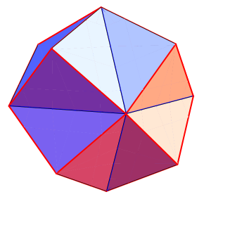
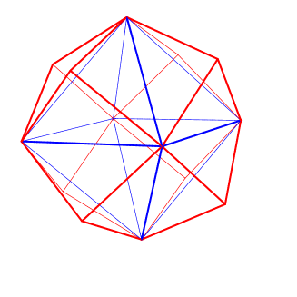
Figure 5: The isohedral triakis octahedron with $r=1.82977\cdots$.

If the vertices of our octahedron $\Omega$ are taken as

$$\mathrm{A}^{\pm}=(\pm 1,0,0),\qquad\mathrm{B}^{\pm}=(0,\pm 1,0),\qquad\mathrm{C}^{\pm}=(0,0,\pm 1),$$ (22)

then the symmetry group of $\Omega$ is the same as that of the cube $C$ in §2, namely, the Weyl group $W(\mathrm{B}_{3})$. It is just the symmetry group $G=G(k)$ of $P(k)$ for every $k=0,1,2,3$ and $r>0$.

Theorem 5.1

For the family of isohedral triakis octahedra, $\mathcal{H}_{G(k)}\varsubsetneq\mathcal{H}_{P(k)}$ if and only if

• $k=0$ and $r=r_{0}:=3\cdot 2^{-3/4}=1.78381\cdots$,

• $k=1$ and $r=r_{1}:=2.24580\cdots$ is the unique positive root of an octic equation

  $$\chi_{1}(r):=16r^{8}+32r^{7}+40r^{6}-48r^{5}-396r^{4}-432r^{3}-810r^{2}-972r-729=0,$$ (23)

• $k=2,3$ and $r=r_{2}=r_{3}:=1.82977\cdots$ is the unique positive root of a quartic equation

  $$\chi_{2}(r):=4r^{4}+8r^{3}+6r^{2}-18r-81=0.$$ (24)

If any of these is the case, then $\dim\mathcal{H}_{G(k)}=48<\dim\mathcal{H}_{P(k)}=96$ and as $\mathbb{R}[\partial]$-modules, $\mathcal{H}_{G(k)}=\mathcal{H}_{\mathrm{B}_{3}}$ is generated by the polynomial $\varDelta_{\mathrm{B}_{3}}(x)$ in formula (15) while $\mathcal{H}_{P(k)}$ is generated by

$$F(x):=\varDelta_{\mathrm{B}_{3}}(x)\cdot\{5(x_{1}^{4}+x_{2}^{4}+x_{3}^{4})-13(x_{1}^{2}x_{2}^{2}+x_{2}^{2}x_{3}^{2}+x_{3}^{2}x_{1}^{2})\}.$$ (25)

As in the case of Theorem 2.1 this theorem is also established through the analysis of PDEs (6). To adjust the notation to the current situation we represent the index sets $I_{0}$, $I_{1}$, $I_{2}$ in §3 by letting the vertices, edges and faces of $P$ to speak of themselves, that is, by setting

$$I_{0} =\{\mathrm{A}^{a},\,\mathrm{B}^{b},\,\mathrm{C}^{c}\}\cup\{\mathrm{D}^{abc}\},$$

$$I_{1} =\{\mathrm{A}^{a}\mathrm{B}^{b},\,\mathrm{A}^{a}\mathrm{C}^{c},\,\mathrm{B}^{b}\mathrm{C}^{c}\}\cup\{\mathrm{A}^{a}\mathrm{D}^{abc},\,\mathrm{B}^{b}\mathrm{D}^{abc},\,\mathrm{C}^{c}\mathrm{D}^{abc}\},$$

$$I_{2} =\{\mathrm{A}^{a}\mathrm{B}^{b}\mathrm{D}^{abc},\,\mathrm{A}^{a}\mathrm{C}^{c}\mathrm{D}^{abc},\,\mathrm{B}^{b}\mathrm{C}^{c}\mathrm{D}^{abc}\},$$

where $a$, $b$, $c$ take $\pm$ signs freely and $\{\cdots\}$ stands for an orbit under symmetries. For an index $\mathrm{A}^{a}\mathrm{B}^{b}\in I_{1}$ the same symbol $\mathrm{A}^{a}\mathrm{B}^{b}$ denotes the foot of orthogonal projection from the origin $\mathrm{O}$ to the affine line passing through $\mathrm{A}^{a}$ and $\mathrm{B}^{b}$; this rule also applies to another index $\mathrm{A}^{a}\mathrm{D}^{abc}\in I_{1}$ as well as to all the other indices of $I_{1}$. Similarly, for an index $\mathrm{A}^{a}\mathrm{B}^{b}\mathrm{D}^{abc}\in I_{2}$ the same symbol $\mathrm{A}^{a}\mathrm{B}^{b}\mathrm{D}^{abc}$ denotes the foot of orthogonal projection from $\mathrm{O}$ to the affine plane passing through $\mathrm{A}^{a}$, $\mathrm{B}^{b}$, $\mathrm{D}^{abc}$, with this rule applying to all the other indices of $I_{2}$; see Figure 4.

Up to symmetries there are three types of vertex-to-edge incidence relations:

$$(\mathrm{VE}1)\quad\mathrm{A}^{+}\prec\mathrm{A}^{+}\mathrm{B}^{+},\qquad(\mathrm{VE}2)\quad\mathrm{A}^{+}\prec\mathrm{A}^{+}\mathrm{D}^{+++},\qquad(\mathrm{VE}3)\quad\mathrm{D}^{+++}\prec\mathrm{A}^{+}\mathrm{D}^{+++}.$$

On the other hand, up to symmetries there are two types of edge-to-face incidence relations:

$$(\mathrm{EF}1)\quad\mathrm{A}^{+}\mathrm{B}^{+}\prec\mathrm{A}^{+}\mathrm{B}^{+}\mathrm{D}^{+++},\qquad(\mathrm{EF}2)\quad\mathrm{A}^{+}\mathrm{D}^{+++}\prec\mathrm{A}^{+}\mathrm{B}^{+}\mathrm{D}^{+++}.$$

The incidence number of an incidence relation depends only on its type. Let $\mathrm{ve}_{\nu}$ denote the incidence number of type ($\mathrm{VE}\nu$), $\nu=1,2,3$, and $\mathrm{ef}_{\nu}$ denote that of type ($\mathrm{EF}\nu$), $\nu=1,2$, respectively. Notice that the presentation around here is quite similar to the presentation around formulas (10) and (11). Indeed the treatment of triakis octahedra will be very parallel to that of triakis tetrahedra, so that the main focus in what follows will be on how one can modify the arguments in the tetrahedral case to the octahedral one.

We consider how Lemma 3.1 can be modified. Since $P$ is $W(\mathrm{B}_{3})$-symmetric, $\tau_{m}^{(k)}(x)$ must be $W(\mathrm{B}_{3})$-invariant and hence can be written in unique ways as polynomials of $e_{2}(x)$, $e_{4}(x)$, $e_{6}(x)$. Note that $\tau_{m}^{(k)}(x)$ is identically zero whenever $m$ is odd. For $m=2,4,6,8$, one can write

$$\begin{split}\tau_{2}^{(k)}(x)&=a_{2}^{(k)}\,e_{2}(x),\\ \tau_{4}^{(k)}(x)&=a_{4}^{(k)}\,e_{4}(x)+b_{4}^{(k)}\,e_{2}^{2}(x),\\ \tau_{6}^{(k)}(x)&=a_{6}^{(k)}\,e_{6}(x)+b_{6}^{(k)}\,e_{2}(x)\,e_{4}(x)+c_{6}^{(k)}\,e_{2}^{3}(x),\\ \tau_{8}^{(k)}(x)&=a_{8}^{(k)}\,e_{4}^{2}(x)+b_{8}^{(k)}\,e_{2}(x)\,e_{6}(x)+c_{8}^{(k)}\,e_{2}^{2}(x)\,e_{4}(x)+d_{8}^{(k)}\,e_{2}^{4}(x).\end{split}$$ (26)

Lemma 5.2

For $k=0,1,2,3$, the following hold:

1. If none of $a_{2}^{(k)}$, $a_{4}^{(k)}$, $a_{6}^{(k)}$ is zero, then the infinite system (6) is equivalent to the finite system (14) so that one has $\mathcal{H}_{P(k)}=\mathcal{H}_{\mathrm{B}_{3}}$.

2. If $a_{4}^{(k)}=0$ but none of $a_{2}^{(k)}$, $a_{6}^{(k)}$, $a_{8}^{(k)}$ is zero, then system (6) is equivalent to

   $$e_{2}(\partial)f=e_{6}(\partial)f=e_{4}^{2}(\partial)f=0.$$ (27)

   If $\mathcal{S}$ denotes the solution space to system (27), then there exists an exact sequence

   $$\begin{CD}0@>{}>{}>\mathcal{H}_{\mathrm{B}_{3}}@>{{\scriptstyle\mathrm{inclusion}}}>{}>\mathcal{S}@>{e_{4}(\partial)}>{}>\mathcal{H}_{\mathrm{B}_{3}}@>{}>{}>0.\end{CD}$$ (28)

   As an $\mathbb{R}[\partial]$-module, $\mathcal{S}$ is generated by the polynomial $F(x)$ defined in formula (25).

Proof. The proof of assertion (1) of this lemma is the same as that of assertion (2) of Lemma 3.1. Under the assumption of assertion (2) of this lemma, the first, third and fourth equations of (26) imply that system (27) leads to $\tau_{2}^{(k)}(\partial)f=\tau_{6}^{(k)}(\partial)f=\tau_{8}^{(k)}(\partial)f=0$ and conversely the latter leads back to the former. Under system (27), equation $\tau_{m}^{(k)}(\partial)f=0$ is redundant for $m=4$ or for any even $m\geq 10$. Indeed, for $m=4$ it is trivial from $a_{4}^{(k)}=0$ and the second equation of (26). For $m\geq 10$ the $W(\mathrm{B}_{3})$-invariance of $\tau_{m}^{(k)}(x)$ allows us to write

$$\tau_{m}^{(k)}(\partial)f=\sum_{2a+4b+6c=m}\alpha_{abc}^{(k)}\cdot e_{2}^{a}(\partial)\cdot e_{4}^{b}(\partial)\cdot e_{6}^{c}(\partial)f,$$

with suitable constants $\alpha_{abc}^{(k)}$. Equations (27) imply that the summand with index $(a,b,c)$ vanishes if either $a\geq 1$, or $b\geq 2$, or $c\geq 1$. Thus the index of a nonzero summand, if any, must satisfy $a=c=0$ and $b\leq 1$ and so $m=2a+4b+6c\leq 2\cdot 0+4\cdot 1+4\cdot 0=4$. Therefore system (6) is equivalent to system (27). Next we verify the exact sequence (28). The inclusion $\mathcal{H}_{\mathrm{B}_{3}}\subset\mathcal{S}$ and the well-definedness of $e_{4}(\partial):\mathcal{S}\to\mathcal{H}_{\mathrm{B}_{3}}$ are obvious since $\mathcal{H}_{\mathrm{B}_{3}}$ is the solution space to system (14) while $\mathcal{S}$ is to system (27). For the same reason sequence (28) is exact at the middle term $\mathcal{S}$. A direct check shows that polynomial $F(x)$ in formula (25) satisfies

$$e_{2}(\partial)F=e_{6}(\partial)F=0,\qquad e_{4}(\partial)F=-15120\varDelta_{\mathrm{B}_{3}}.$$

Hence $F\in\mathcal{S}$ and $e_{4}(\partial)$ sends $F$ to $\varDelta_{\mathrm{B}_{3}}$ up to a nonzero constant multiple. Thus $e_{4}(\partial):\mathcal{S}\to\mathcal{H}_{\mathrm{B}_{3}}$ is surjective, since it is an $\mathbb{R}[\partial]$-homomorphism and $\varDelta_{\mathrm{B}_{3}}$ generates $\mathcal{H}_{\mathrm{B}_{3}}$ as an $\mathbb{R}[\partial]$-module. Finally we show that $F$ generates $\mathcal{S}$ as an $\mathbb{R}[\partial]$-module. For any $f\in\mathcal{S}$, consider $e_{4}(\partial)f\in\mathcal{H}_{\mathrm{B}_{3}}$. There is a polynomial $\varphi(x)$ such that $e_{4}(\partial)f=-15120\,\varphi(\partial)\varDelta_{\mathrm{B}_{3}}$. Then $g:=f-\varphi(\partial)F\in\mathcal{S}$ satisfies $e_{4}(\partial)g=e_{4}(\partial)f-\varphi(\partial)e_{4}(\partial)F=e_{4}(\partial)f+15120\,\varphi(\partial)\varDelta_{\mathrm{B}_{3}}=0$. Exact sequence (28) tells us that $g\in\mathcal{H}_{\mathrm{B}_{3}}$ and so there is a polynomial $\psi(x)$ such that $g=-15120\,\psi(\partial)\varDelta_{\mathrm{B}_{3}}=\psi(\partial)e_{4}(\partial)F$. Now if $\eta(x):=\varphi(x)+\psi(x)e_{4}(x)$ then $f=\eta(\partial)F$. This proves the last claim. $\Box$

6 Skeletons of Triakis Octahedra

Lemma 5.2 is applied to each skeleton of the triakis octahedron to establish Theorem 5.1.

6.1 Vertex Problem

Formula (17) for triakis tetrahedra carries over to the case of triakis octahedra, but this time formula (18) should be replaced by

$$\tau_{1,m}^{(0)}(x)=\sum_{a}\langle\mathrm{A}^{a},\,x\rangle^{m}+\sum_{b}\langle\mathrm{B}^{b},\,x\rangle^{m}+\sum_{c}\langle\mathrm{C}^{c},\,x\rangle^{m},\quad\tau_{2,m}^{(0)}(x)=\sum_{(a,b,c)}\langle\mathrm{D}^{abc},\,x\rangle^{m},$$

where the sums are taken over all $a,b,c=\pm$. Using the coordinates (22) and the relation $\mathrm{D}^{abc}=r(\mathrm{A}^{a}+\mathrm{B}^{b}+\mathrm{C}^{c})/3$, one finds in formulas (26),

$$a_{2}^{(0)} =\frac{8}{9}r^{2}+2>0, a_{4}^{(0)} =\frac{32}{81}\left(r^{4}-\frac{3^{4}}{2^{3}}\right),$$

$$a_{6}^{(0)} =\frac{2}{243}(4r^{2}+9)(16r^{4}-36r^{2}+81)>0, a_{8}^{(0)} =\frac{128}{6561}r^{8}+4>0.$$

Note that $a_{4}^{(0)}=0$ if and only if $r=r_{0}:=3\cdot 2^{-3/4}=1.78381\cdots$. Thus if $r=r_{0}$ then assertion (2) of Lemma 5.2 yields $\mathcal{H}_{P(0)}=\mathcal{S}$, while if $r\neq r_{0}$ then assertion (1) of Lemma 5.2 yields $\mathcal{H}_{P(0)}=\mathcal{H}_{\mathrm{B}_{3}}$. One has $\mathcal{H}_{G(0)}\varsubsetneq\mathcal{H}_{P(0)}$ only when $r=r_{0}$. This proves Theorem 5.1 for $k=0$.

6.2 Edge Problem

It is obvious that for an index $\mathrm{A}^{a}\mathrm{B}^{b}\in I_{1}$, the corresponding foot is $\mathrm{A}^{a}\mathrm{B}^{b}=(\mathrm{A}^{a}+\mathrm{B}^{b})/2$ with this rule applying to every index of the same type. For indices of the other type in $I_{1}$, one finds

$$\mathrm{A}^{a}\mathrm{D}^{abc}=(au,\,bv,\,cv),\qquad\mathrm{B}^{b}\mathrm{D}^{abc}=(av,\,bu,\,cv),\qquad\mathrm{C}^{c}\mathrm{D}^{abc}=(av,\,bv,\,cu),$$

with $a,b,c=\pm$, where

$$u:=\frac{2r^{2}}{3(r^{2}-2r+3)},\qquad v:=\frac{r(3-r)}{3(r^{2}-2r+3)}.$$

Formula (19) remains true for triakis octahedra if formulas in Table 1 are replaced by

$$\begin{split}\tau_{1,m}^{(1)}(x)&=\sum h_{m}(\mathrm{A}^{a},\mathrm{A}^{a}\mathrm{B}^{b})+\sum h_{m}(\mathrm{A}^{a},\mathrm{A}^{a}\mathrm{C}^{c})+\sum h_{m}(\mathrm{B}^{b},\mathrm{A}^{a}\mathrm{B}^{b})\\ &+\sum h_{m}(\mathrm{B}^{b},\mathrm{B}^{b}\mathrm{C}^{c})+\sum h_{m}(\mathrm{C}^{c},\mathrm{A}^{a}\mathrm{C}^{c})+\sum h_{m}(\mathrm{C}^{c},\mathrm{B}^{b}\mathrm{C}^{c}),\\ \tau_{2,m}^{(1)}(x)&=\sum h_{m}(\mathrm{A}^{a},\mathrm{A}^{a}\mathrm{D}^{abc})+\sum h_{m}(\mathrm{B}^{b},\mathrm{B}^{b}\mathrm{D}^{abc})+\sum h_{m}(\mathrm{C}^{c},\mathrm{C}^{c}\mathrm{D}^{abc}),\\ \tau_{3,m}^{(1)}(x)&=\sum h_{m}(\mathrm{D}^{abc},\mathrm{A}^{a}\mathrm{D}^{abc})+\sum h_{m}(\mathrm{D}^{abc},\mathrm{B}^{b}\mathrm{D}^{abc})+\sum h_{m}(\mathrm{D}^{abc},\mathrm{C}^{c}\mathrm{D}^{abc}).\end{split}$$

The three types of vertex-to-edge incidence numbers are evaluated as

$$\mathrm{ve}_{1}=\frac{1}{\sqrt{2}},\qquad\mathrm{ve}_{2}=\frac{3-r}{\sqrt{3(r^{2}-2r+3)}},\qquad\mathrm{ve}_{3}=\frac{r(r-1)}{\sqrt{3(r^{2}-2r+3)}}.$$ (29)

Putting all these informations together into formulas (26), one finds

$$a_{2}^{(1)} =8\sqrt{2}+\frac{8}{9}(r^{2}+r+3)\sqrt{3(r^{2}-2r+3)}>0,$$

$$a_{4}^{(1)} =-12\sqrt{2}+\frac{16}{81}(2r^{4}+2r^{3}-9r-27)\sqrt{3(r^{2}-2r+3)},$$

$$a_{6}^{(1)} =12\sqrt{2}+\frac{8}{243}(16r^{6}+16r^{5}-18r^{3}+81r+243)\sqrt{3(r^{2}-2r+3)}>0,$$

$$a_{8}^{(1)} =12\sqrt{2}+\frac{16}{6561}(8r^{8}+8r^{7}-36r^{5}-108r^{4}-162r^{3}+729r+2187)\sqrt{3(r^{2}-2r+3)}.$$

Observe that $a_{2}^{(1)}$ and $a_{6}^{(1)}$ are positive for every $r>0$. Indeed the former is obvious and the latter follows from the fact that $\psi(r):=16r^{6}+16r^{5}-18r^{3}+81r+243$ has a positive value $\psi(0)=243$ at $r=0$ and a positive derivative $\psi^{\prime}(r)=96r^{5}+71r^{4}+(3r^{2}-9)^{2}$ for every $r>0$. On the other hand, there exists a unique positive number $r=r_{1}$ at which $a_{4}^{(1)}=0$, because

$$a_{4}^{(1)}=-4(4+3\sqrt{2})<0\quad\mbox{at \,\, $r=0$};\qquad\frac{da_{4}^{(1)}}{dr}=\frac{160r^{3}(r^{2}-r+1)}{27\sqrt{3(r^{2}-2r+3)}}>0\quad\mbox{for \,\, $r>0$},$$

and $a_{4}^{(1)}$ tends to $+\infty$ as $r\to+\infty$. If $\chi_{1}(r)$ is the octic polynomial defined in formula (23),

$$a_{4}^{(1)}\left\{12\sqrt{2}+\frac{16}{81}(2r^{4}+2r^{3}-9r-27)\sqrt{3(r^{2}-2r+3)}\right\}=\frac{32}{2187}(2r^{2}-4r+3)\,\chi_{1}(r).$$

So $r_{1}=2.24580\cdots$ is the unique positive root of octic equation $\chi_{1}(r)=0$. Note that $a_{8}^{(1)}=54.1247\cdots$ is nonzero at $r=r_{1}$. Thus Lemma 5.2 leads to Theorem 5.1 for $k=1$.

6.3 Face Problem

For each index of $I_{2}$, the foot on the corresponding affine plane is given by

$$\mathrm{A}^{a}\mathrm{B}^{b}\mathrm{D}^{abc}=(aq,\,bq,\,cp),\qquad\mathrm{A}^{a}\mathrm{C}^{c}\mathrm{D}^{abc}=(aq,\,bp,\,cq),\qquad\mathrm{B}^{b}\mathrm{C}^{c}\mathrm{D}^{abc}=(ap,\,bq,\,cq),$$

with $a,b,c=\pm$, where

$$p:=\frac{r(3-2r)}{3(2r^{2}-4r+3)},\qquad q:=\frac{r^{2}}{3(2r^{2}-4r+3)}.$$

Observe that up to symmetries there are three types of vertex-edge-face flags:

$$(1) \mathrm{A}^{+}\prec\mathrm{A}^{+}\mathrm{B}^{+}\prec\mathrm{A}^{+}\mathrm{B}^{+}\mathrm{D}^{+++} (\mathrm{VE}1)\,\,\&\,\,(\mathrm{EF}1),$$

$$(2) \mathrm{A}^{+}\prec\mathrm{A}^{+}\mathrm{D}^{+++}\prec\mathrm{A}^{+}\mathrm{B}^{+}\mathrm{D}^{+++} (\mathrm{VE}2)\,\,\&\,\,(\mathrm{EF}2),$$

$$(3) \mathrm{D}^{+++}\prec\mathrm{A}^{+}\mathrm{D}^{+++}\prec\mathrm{A}^{+}\mathrm{B}^{+}\mathrm{D}^{+++} (\mathrm{VE}3)\,\,\&\,\,(\mathrm{EF}2).$$

Formula (21) remains true for triakis octahedra if formulas in Table 2 are replaced by

$$\tau_{1,m}^{(2)}(x) =\sum h_{m}(\mathrm{A}^{a},\mathrm{A}^{a}\mathrm{B}^{b},\mathrm{A}^{a}\mathrm{B}^{b}\mathrm{D}^{abc})+\cdots \mbox{sum over flags of type (1)},$$

$$\tau_{2,m}^{(2)}(x) =\sum h_{m}(\mathrm{A}^{a},\mathrm{A}^{a}\mathrm{D}^{abc},\mathrm{A}^{a}\mathrm{B}^{b}\mathrm{D}^{abc})+\cdots \mbox{sum over flags of type (2)},$$

$$\tau_{3,m}^{(2)}(x) =\sum h_{m}(\mathrm{D}^{abc},\mathrm{A}^{a}\mathrm{D}^{abc},\mathrm{A}^{a}\mathrm{B}^{b}\mathrm{D}^{abc})+\cdots \mbox{sum over flags of type (3)}.$$

While the vertex-to-edge incidence numbers are given in (29), the edge-to-face ones are

$$\mathrm{ef}_{1}=\frac{3-2r}{\sqrt{6(2r^{2}-4r+3)}},\qquad\mathrm{ef}_{2}=\frac{r(r-1)}{\sqrt{(r^{2}-2r+3)(2r^{2}-4r+3)}}.$$

So upon multiplying by a nonzero constant simultaneously, one may put

$$\mathrm{ve}_{1}\cdot\mathrm{ef}_{1} =\frac{3-2r}{2(2r^{2}-4r+3)},\qquad \mathrm{ve}_{2}\cdot\mathrm{ef}_{2} =\frac{(3-r)r(r-1)}{(r^{2}-2r+3)(2r^{2}-4r+3)},$$

$$\mathrm{ve}_{3}\cdot\mathrm{ef}_{2} =\frac{r^{2}(r-1)^{2}}{(r^{2}-2r+3)(2r^{2}-4r+3)}.$$

Putting all these informations together into formulas (26), one finds

$$a_{2}^{(2)} =\frac{8}{3}(r^{2}+2r+6)>0,\qquad a_{4}^{(2)}=\frac{8}{27}\,\chi_{2}(r),$$

$$a_{6}^{(2)} =\frac{8}{81}(16r^{6}+32r^{5}+24r^{4}-18r^{3}-54r^{2}+243)>0,$$

$$a_{8}^{(2)} =\frac{8}{2187}(16r^{8}+32r^{7}+24r^{6}-72r^{5}-324r^{4}-648r^{3}-486r^{2}+1458r+6561),$$

where $\chi_{2}(r)$ is the quartic polynomial defined in (24). Observe that $a_{2}^{(2)}$ and $a_{6}^{(2)}$ are positive for every $r>0$. Indeed the former is obvious and latter follows from the fact that $a_{6}^{(2)}$ $(r\geq 0)$ attains its minimum $22.0304\cdots>0$ at $r=0.743471\cdots$. Note that $a_{4}^{(2)}=0$ if and only if $r$ is the unique positive root $r_{2}=1.82977\cdots$ of equation (24), at which $a_{8}^{(2)}=13.2853\cdots$ is nonzero. Lemma 5.2 thus leads to Theorem 5.1 for $k=2$.

By [5, Theorem 2.2] the volume problem ($k=3$) has the same solution as the face problem ($k=2$), since $P$ is isohedral. The proof of Theorem 5.1 is now complete.

It is an interesting exercise left behind to deal with a similar problem for isohedral triakis icosahedra. It would also be interesting if such special solids as discussed in this article appear in nature and physical sciences.

References

- [1] E. Catalan, Mémoire sur la théorie des polyèdres, J. École Polytechnique (Paris) 41 (1865), 1–71.
- [2] B. Grünbaum, Graphs of polyhedra; polyhedra as graphs, Discrete Math. 307 (2007), no. 3-5, 445–463.
- [3] B. Grünbaum and G.C. Shephard, Isohedra with nonconvex faces, J. Geom. 63 (1998), no. 1-2, 76–96.
- [4] S. Helgason, Groups and geometric analysis, Academic Press, Orlando, 1984.
- [5] K. Iwasaki, Polytopes and the mean value property, Discrete Comput. Geom. 17 (1997), no. 2, 163–189.
- [6] K. Iwasaki, Cubic harmonics and Bernoulli numbers, J. Combin. Theory, Ser. A 119 (2012), no. 6, 1216–1234.
- [7] M. Koca, N. Ozdes Koca and R. Koç, Catalan solids derived from three-dimensional-root systems and quaternions, J. Math. Phys. 51 (2010), no. 4, 043501, 14 pp.
- [8] I.G. Macdonald, Symmetric functions and Hall polynomials, 2nd ed., Oxford Univ. Press, Oxford, 1995.
- [9] R. Steinberg, Differential equations invariant under finite reflection groups, Trans. Amer. Math. Soc. 112 (1964), no. 3, 392–400.