A Fast Iterative Algorithm for Recovery of Sparse Signals from One-Bit Quantized Measurements

Abstract

This paper considers the problem of reconstructing sparse or compressible signals from one-bit quantized measurements. We study a new method that uses a log-sum penalty function, also referred to as the Gaussian entropy, for sparse signal recovery. Also, in the proposed method, sigmoid functions are introduced to quantify the consistency between the acquired one-bit quantized data and the reconstructed measurements. A fast iterative algorithm is developed by iteratively minimizing a convex surrogate function that bounds the original objective function, which leads to an iterative reweighted process that alternates between estimating the sparse signal and refining the weights of the surrogate function. Connections between the proposed algorithm and other existing methods are discussed. Numerical results are provided to illustrate the effectiveness of the proposed algorithm.

I Introduction

Conventional compressed sensing framework recovers a sparse signal $\boldsymbol{x}\in\mathbb{R}^{n}$ from only a few linear measurements:

$$\boldsymbol{y}=\boldsymbol{A}\boldsymbol{x}$$ (1)

where $\boldsymbol{y}\in\mathbb{R}^{m}$ denotes the acquired measurements, $\boldsymbol{A}\in\mathbb{R}^{m\times n}$ is the sampling matrix, and $m\ll n$. Such a problem has been extensively studied and a variety of algorithms that provide consistent recovery performance guarantee were proposed, e.g. [1, 2, 3]. In practice, however, measurements have to be quantized before being further processed. Moreover, in distributed systems where data acquisition is limited by bandwidth and energy constraints, aggressive quantization strategies which compress real-valued measurements into one or only a few bits of data are preferred. This has inspired recent interest in studying compressed sensing based on quantized measurements. Specifically, in this paper, we are interested in an extreme case where each measurement is quantized into one bit of information

$$\boldsymbol{b}=\text{sign}(\boldsymbol{y})=\text{sign}(\boldsymbol{A}\boldsymbol{x})$$ (2)

where “sign” denotes an operator that performs the sign function element-wise on the vector, the sign function returns $1$ for positive numbers and $-1$ otherwise. Clearly, in this case, only the sign of the measurement is retained while the information about the magnitude of the signal is lost. This makes an exact reconstruction of the sparse signal $\boldsymbol{x}$ impossible. Nevertheless, if we impose a unit-norm on the sparse signal, it has been shown [4, 5] that signals can be recovered with a bounded error from one bit quantized data. Besides, in many practical applications such as source localization, direction-of-arrival estimation, and chemical agent detection, it is the locations of the nonzero components of the sparse signal, other than the amplitudes of the signal components, that have significant physical meanings and are of our ultimate concern. Recent results [6] show that asymptotic reliable recovery of the support of sparse signals is possible even with only one-bit quantized data.

The problem of recovering a sparse or compressible signal from one-bit measurements was firstly introduced by Boufounos and Baraniuk in their work [7]. Following that, the reconstruction performance from one-bit measurements was more thoroughly studied [4, 5, 6, 8] and a variety of one-bit compressed sensing algorithms such as binary iterative hard thresholding (BIHT) [4], matching sign pursuit (MSP) [9], $l_{1}$ minimization-based linear programming (LP) [5], and restricted-step shrinkage (RSS) [10] were proposed. Although achieving good reconstruction performance, these algorithms either require the knowledge of the sparsity level [4, 9] or are $l_{1}$-based methods that often yield solutions that are not necessarily the sparsest [5, 10]. In this paper, we study a new method that uses the Gaussian entropy-based penalty function for sparse signal recovery. The Gaussian entropy has the potential to be much more sparsity-encouraging than the $l_{1}$ norm. By resorting to a bound optimization approach, we propose an iterative reweighted algorithm that successively minimizes a sequence of convex surrogate functions with its weights for the next iteration computed based on the current estimate. The proposed algorithm has the advantage that it does not need the cardinality of the support set, $K$, of the sparse signal. Moreover, our analysis and simulation results show that the proposed algorithm outperforms the $l_{1}$-type methods [5, 10] in identifying the support set of the sparse signal.

II One-Bit Compressed Sensing

Since the only information we have about the original signal is the sign of the measurements, we hope that the reconstructed signal $\boldsymbol{\hat{x}}$ yields estimated measurements that are consistent with our knowledge, that is

$$\text{sign}(\boldsymbol{a}_{i}^{T}\boldsymbol{\hat{x}})=b_{i}\qquad\forall i$$ (3)

or in other words

$$b_{i}\boldsymbol{a}_{i}^{T}\boldsymbol{\hat{x}}\geq 0\qquad\forall i$$ (4)

where $\boldsymbol{a}_{i}$ denotes the transpose of the $i$th row of the sampling matrix $\boldsymbol{A}$, $b_{i}$ is the $i$th element of the sign vector $\boldsymbol{b}$. This consistency can be enforced by hard constraints [5, 10] or can be quantified by a well-defined metric which is meant to be maximized/minimized [9, 4, 11]. In this paper, we introduce the sigmoid function to quantify the consistency between what we acquired and what we estimated. The metric is defined as

$$\phi(\boldsymbol{x})\triangleq\sum_{i=1}^{m}\log(\sigma(b_{i}\boldsymbol{a}_{i}^{T}\boldsymbol{x}))$$ (5)

where

$$\sigma(x)\triangleq\frac{1}{1+\exp(-x)}$$

is the sigmoid function. The sigmoid function, with an ‘S’ shape, approaches one for positive $x$ and zero for negative $x$. Hence it is a good measure to evaluate the consistency between $b_{i}$ and $\boldsymbol{a}_{i}^{T}\boldsymbol{x}$. Also, the sigmoid function, differentiable and log-concave, is more amiable for algorithm development than the indicator function adopted in [9, 4, 11]. Note that the sigmoid function, also referred to as the logistic regression model, has been widely used in statistics and machine learning to represent the posterior class probability.

Naturally our objective is to find $\boldsymbol{x}$ to maximize the consistency between the acquired data and the reconstructed measurements, i.e.

$$\max_{\boldsymbol{x}}\qquad\phi(\boldsymbol{x})=\sum_{i=1}^{m}\log(\sigma(b_{i}\boldsymbol{a}_{i}^{T}\boldsymbol{x}))$$ (6)

This optimization, however, does not necessarily lead to a sparse solution. To obtain sparse solutions, a sparsity-encouraging term needs to be incorporated to encourage sparsity of the signal coefficients. The most commonly used sparsity-encouraging penalty function is $l_{1}$ norm. An attractive property of the $l_{1}$ norm is its convexity, which makes the $l_{1}$-based minimization a well-behaved numerical problem. Despite its popularity, $l_{1}$ type methods suffer from the drawback that the global minimum does not necessarily coincide with the sparsest solution, particularly when only a few measurements are available for signal reconstruction. In this paper, we consider the use of an alternative sparsity-encouraging penalty function for sparse signal recovery. This penalty function, also referred to as the Gaussian entropy, is defined as

$$h_{G}(\boldsymbol{x})=\sum_{i=1}^{n}\log|x_{i}|^{2}$$ (7)

where $x_{i}$ denotes the $i$th component of the vector $\boldsymbol{x}$. Such a log-sum penalty function was firstly introduced in [12] for basis selection. This penalty function has the potential to be much more sparsity-encouraging than the $l_{1}$ norm. It can be readily observed that the log-sum (Gaussian entropy) penalty function, like $l_{0}$ norm, has infinite slope at $x_{i}=0,\forall i$, which implies that a relatively large penalty is placed on small nonzero coefficients to drive them to zero. The reason why the Gaussian entropy is more sparsity-encouraging than $l_{1}$ function will also be explained from an algorithmic perspective later in our paper. Using this penalty function, the problem of finding a sparse solution to maximize the consistency can be formulated as follows

$$\hat{\boldsymbol{x}} =\arg\min L(\boldsymbol{x})$$

$$=\arg\min_{\boldsymbol{x}}-\sum_{i=1}^{m}\log(\sigma(b_{i}\boldsymbol{x}^{T}\boldsymbol{a}_{i}))+\lambda\sum_{i=1}^{n}\log|x_{i}|^{2}$$ (8)

where $\lambda$ is a parameter controlling the trade-off between the degree of sparsity and the quality of consistency.

II-A Proposed Iterative Algorithm

Due to the concave and unbounded nature of the Gaussian entropy, the objective function (8) is non-convex and unbounded from below. Instead of resorting to the gradient descend method, we propose an iterative reweighted algorithm which provides fast convergence and guarantees that every iteration results in a decreasing objective function value. The algorithm is developed based on a bound optimization approach [14]. The idea is to construct a surrogate function $Q(\boldsymbol{x}|\boldsymbol{\hat{x}}^{(t)})$ such that

$$Q(\boldsymbol{x}|\boldsymbol{\hat{x}}^{(t)})-L(\boldsymbol{x})\geq 0$$ (9)

and the minimum is attained when $\boldsymbol{x}=\boldsymbol{\hat{x}}^{(t)}$, i.e. $Q(\boldsymbol{\hat{x}}^{(t)}|\boldsymbol{\hat{x}}^{(t)})=L(\boldsymbol{\hat{x}}^{(t)})$. Optimizing $L(\boldsymbol{x})$ can therefore be replaced by minimizing the surrogate function $Q(\boldsymbol{x}|\boldsymbol{\hat{x}}^{(t)})$ iteratively. Suppose that

$$\boldsymbol{\hat{x}}^{(t+1)}=\min_{\boldsymbol{x}}Q(\boldsymbol{x}|\boldsymbol{\hat{x}}^{(t)})$$

We can ensure that

$$L(\boldsymbol{\hat{x}}^{(t+1)})= L(\boldsymbol{\hat{x}}^{(t+1)})-Q(\boldsymbol{\hat{x}}^{(t+1)}|\boldsymbol{\hat{x}}^{(t)})+Q(\boldsymbol{\hat{x}}^{(t+1)}|\boldsymbol{\hat{x}}^{(t)})$$

$$< L(\boldsymbol{\hat{x}}^{(t)})-Q(\boldsymbol{\hat{x}}^{(t)}|\boldsymbol{\hat{x}}^{(t)})+Q(\boldsymbol{\hat{x}}^{(t+1)}|\boldsymbol{\hat{x}}^{(t)})$$

$$\leq L(\boldsymbol{\hat{x}}^{(t)})-Q(\boldsymbol{\hat{x}}^{(t)}|\boldsymbol{\hat{x}}^{(t)})+Q(\boldsymbol{\hat{x}}^{(t)}|\boldsymbol{\hat{x}}^{(t)})$$

$$= L(\boldsymbol{\hat{x}}^{(t)})$$ (10)

where the first inequality follows from the fact that $Q(\boldsymbol{x}|\boldsymbol{\hat{x}}^{(t)})-L(\boldsymbol{x})$ attains its minimum when $\boldsymbol{x}=\boldsymbol{\hat{x}}^{(t)}$; the second inequality comes by noting that $Q(\boldsymbol{x}|\boldsymbol{\hat{x}}^{(t)})$ is minimized at $\boldsymbol{x}=\boldsymbol{\hat{x}}^{(t+1)}$. We see that, through minimizing the surrogate function iteratively, the objective function $L(\boldsymbol{x})$ is guaranteed to decrease at each iteration.

We now discuss how to find a surrogate function for the original problem (8). Ideally, we hope that the surrogate function is differentiable and convex so that the minimization of the surrogate function is a well-behaved numerical problem. Since the consistency evaluation term is convex, our objective is to find a convex surrogate function for the Gaussian entropy defined in (7). An appropriate choice of such a surrogate function has a quadratic form and is given by

$$f(\boldsymbol{x}|\boldsymbol{\hat{x}}^{(t)})\triangleq\sum_{i=1}^{n}\bigg{(}\frac{x_{i}^{2}}{(\hat{x}_{i}^{(t)})^{2}}+\log(\hat{x}_{i}^{(t)})^{2}-1\bigg{)}$$ (11)

It can be easily verified that

$$f(\boldsymbol{x}|\boldsymbol{\hat{x}}^{(t)})-h_{G}(\boldsymbol{x})\geq 0$$ (12)

with the minimum $0$ attained when $\boldsymbol{x}=\boldsymbol{\hat{x}}^{(t)}$. Therefore the convex function $f(\boldsymbol{x}|\boldsymbol{\hat{x}}^{(t)})$ is a desired surrogate function for the Gaussian entropy $h_{G}(\boldsymbol{x})$. As a consequence, the surrogate function for the objective function $L(\boldsymbol{x})$ is given by

$$Q(\boldsymbol{x}|\boldsymbol{\hat{x}}^{(t)})$$

$$= -\sum_{i=1}^{m}\log(\sigma(b_{i}\boldsymbol{x}^{T}\boldsymbol{a}_{i}))+\lambda\sum_{i=1}^{n}\bigg{(}\frac{x_{i}^{2}}{(\hat{x}_{i}^{(t)})^{2}}+\log(\hat{x}_{i}^{(t)})^{2}-1\bigg{)}$$

$$= -\sum_{i=1}^{m}\log(\sigma(b_{i}\boldsymbol{x}^{T}\boldsymbol{a}_{i}))+\lambda\boldsymbol{x}^{T}\boldsymbol{D}(\boldsymbol{\hat{x}}^{(t)})\boldsymbol{x}+\text{constant}$$ (13)

where

$$\boldsymbol{D}(\boldsymbol{\hat{x}}^{(t)})\triangleq\text{diag}\left\{(\hat{x}_{1}^{(t)})^{-2},\ldots,(\hat{x}_{n}^{(t)})^{-2}\right\}$$

Optimizing $L(\boldsymbol{x})$ now reduces to minimizing the surrogate function $Q(\boldsymbol{x}|\boldsymbol{\hat{x}}^{(t)})$ iteratively. For clarity, the iterative algorithm is briefly summarized as follows.

1. Given an initialization $\boldsymbol{\hat{x}}^{(0)}$.

2. At iteration $t>0$, minimize $Q(\boldsymbol{x}|\boldsymbol{\hat{x}}^{(t)})$, which yields a new estimate $\boldsymbol{\hat{x}}^{(t+1)}$. Based on this new estimate, construct a new surrogate function $Q(\boldsymbol{x}|\boldsymbol{\hat{x}}^{(t+1)})$.

3. Go to Step 2 if $\|\boldsymbol{\hat{x}}^{(t+1)}-\boldsymbol{\hat{x}}^{(t)}\|_{2}>\epsilon$, where $\epsilon$ is a prescribed tolerance value; otherwise stop.

Remark 1: The second step involves optimization of the surrogate function $Q(\boldsymbol{x}|\boldsymbol{\hat{x}}^{(t)})$. Since the surrogate function is differentiable and convex, minimization of $Q(\boldsymbol{x}|\boldsymbol{\hat{x}}^{(t)})$ is a well-behaved numerical problem. Any gradient-based search such as Newton’s method which has a fast convergence rate can be used and is guaranteed to converge to the global maximum.

Remark 2: The above algorithm results in a non-increasing objective function value of $L(\boldsymbol{x})$. In this manner, the iterative algorithm eventually converges to a local minimum of $L(\boldsymbol{x})$. It should be emphasized that the cost function $L(\boldsymbol{x})$ is non-convex. Therefor it is important to choose a suitable starting point for the algorithm. Our simulations suggest that initializing with $\boldsymbol{\hat{x}}^{(0)}=\boldsymbol{A}^{T}\boldsymbol{b}$ usually delivers good reconstruction performance. Moreover, we found from our simulations that, despite starting from different (randomly generated) initial points, if the number of bits, $m$, is sufficiently large, the support of the reconstructed sparse solution is guaranteed to coincide with, or at least be a subset of, the true support of the sparse signal $\boldsymbol{x}$.

Remark 3: The proposed iterative algorithm can be considered as composed of two alternating steps. First, we estimate $\boldsymbol{x}$ through minimizing the current surrogate function $Q(\boldsymbol{x}|\boldsymbol{\hat{x}}^{(t)})$. Second, based on the estimate of $\boldsymbol{x}$, we update the weights of the weighted $l_{2}$ norm penalty of the surrogate function. This alternating process finally results in sparse solutions. To see this, note that the weighted $l_{2}$ norm of $\boldsymbol{x}$ has their weights specified as $\{(\hat{x}_{i}^{(t)})^{-2}\}$. The penalty term has the tendency to decrease these entries in $\boldsymbol{x}$ whose corresponding weights are large, i.e., whose current estimates $\{\hat{x}_{i}^{(t)}\}$ are already small. This negative feedback mechanism keeps suppressing these entries until they reach machine precision and becomes zeros, while leaving only a few prominent nonzero entries survived to meet the consistency requirement.

III Related Work

Our developed algorithm has a close connection with the FOcal Underdetermined System Solver (FOCUSS) algorithm [15] since the latter algorithm also uses an iterative reweighted approach to find sparse solutions to underdetermined systems $\boldsymbol{y}=\boldsymbol{A}\boldsymbol{x}$. Specifically, at each iteration, FOCUSS solves a reweighted $l_{2}$ minimization with weights $w_{i}^{(t+1)}=1/|x_{i}^{(t)}|^{p}$, where $p\in[1\phantom{0}2]$. It was also shown that when $p=2$, FOCUSS is equivalent to a modified Newton’s method minimizing the Gaussian entropy function. As compared with FOCUSS, our paper considers a more general framework in which the data model allows measurement errors/noise and is not confined to be linear, and a general connection between the sparsity-promoting penalty function and the iterative reweighted process is established through the use of the surrogate function. In [16], a similar iterative reweighted algorithm was proposed to enhance sparsity of recovered signals. The algorithm consists of solving a sequence of weighted $l_{1}$-minimization problems with its weights for the next iteration computed based on the current estimate. Such an algorithm, interestingly, is also shown closely related to the log-sum penalty function, i.e. the Gaussian entropy function.

We now explore the relationship between our proposed algorithm and the $l_{1}$-minimization type methods. Following (8), we can formulate a $l_{1}$ norm-based sparsity-promoting optimization

$$\hat{\boldsymbol{x}} =\arg\min_{\boldsymbol{x}}\tilde{L}(\boldsymbol{x})$$

$$=\arg\min_{\boldsymbol{x}}-\sum_{i=1}^{m}\log(\sigma(b_{i}\boldsymbol{x}^{T}\boldsymbol{a}_{i}))+\lambda\sum_{i=1}^{n}|x_{i}|$$ (14)

Similarly, a surrogate function can be constructed to bound the above optimization, from which an iterative algorithm can be developed to solve (14). Note that the $l_{1}$ function $|x|$ can also be upper bounded by a quadratic function. It can be readily verified that the surrogate function for $l_{1}$ norm is given by

$$\tilde{f}(\boldsymbol{x}|\boldsymbol{\hat{x}}^{(t)})\triangleq\frac{1}{2}\sum_{i=1}^{n}\bigg{(}\frac{x_{i}^{2}}{|\hat{x}_{i}^{(t)}|}+|\hat{x}_{i}^{(t)}|\bigg{)}$$ (15)

Therefore the solution to (14) can be found by iteratively minimizing the following surrogate function

$$\tilde{Q}(\boldsymbol{x}|\boldsymbol{\hat{x}}^{(t)})$$

$$= -\sum_{i=1}^{m}\log(\sigma(b_{i}\boldsymbol{x}^{T}\boldsymbol{a}_{i}))+\frac{\lambda}{2}\sum_{i=1}^{n}\bigg{(}\frac{x_{i}^{2}}{|\hat{x}_{i}^{(t)}|}+|\hat{x}_{i}^{(t)}|\bigg{)}$$

$$= -\sum_{i=1}^{m}\log(\sigma(b_{i}\boldsymbol{x}^{T}\boldsymbol{a}_{i}))+\frac{\lambda}{2}\boldsymbol{x}^{T}\boldsymbol{\tilde{D}}(\boldsymbol{\hat{x}}^{(t)})\boldsymbol{x}+\text{constant}$$ (16)

where

$$\boldsymbol{\tilde{D}}(\boldsymbol{\hat{x}}^{(t)})\triangleq\text{diag}\bigg{\{}\frac{1}{|\hat{x}_{1}^{(t)}|},\ldots,\frac{1}{|\hat{x}_{n}^{(t)}|}\bigg{\}}$$

The surrogate function $\tilde{Q}(\boldsymbol{x}|\boldsymbol{\hat{x}}^{(t)})$ has a similar form as (13), except that the surrogate function for the Gaussian entropy updates its weights using $(\hat{x}_{i}^{(t)})^{-2}$, while the surrogate function for the $l_{1}$ norm updates its weights with $(|\hat{x}_{i}^{(t)}|)^{-1}$. This seemingly slight difference, however, results in very different convergence behavior. The latter update equation guarantees converging to a unique global minimum. On the other hand, the update method used in our algorithm renders a more intense effect in de-emphasizing the entries in $\boldsymbol{x}$. Therefore the proposed algorithm is more sparsity-encouraging than the $l_{1}$ type methods, and generally yields a more sparse solution.

IV Numerical Results

We now carry out experiments to illustrate the performance of our proposed one-bit compressed sensing algorithm. In our simulations, the $K$-sparse signal is randomly generated with the support set of the sparse signal randomly chosen according to a uniform distribution. The signals on the support set are independent and identically distributed (i.i.d.) Gaussian random variables with zero mean and unit variance. The measurement matrix $\boldsymbol{A}\in\mathbb{R}^{m\times n}$ is randomly generated with each entry independently drawn from Gaussian distribution with zero mean and unit variance, and then each column of $\boldsymbol{A}$ is normalized to unity for algorithm stability. We compare our proposed algorithm with the other two algorithms, namely, the $l_{1}$ minimization-based linear programming (LP) algorithm [5] (referred to as “one-bit LP”), and the iterative algorithm proposed in Section III to solve the optimization (14) (referred to as “L1-optimization (14)”). Both the latter two algorithms are $l_{1}$ type methods, with the consistency evaluated by different criteria.

We investigate the support recovery performance of respective algorithms. Support recovery accuracy are measured by the false alarm (misidentified) rate and the miss rate. A false alarm event represents the case where coefficients that are zero in the original signal are misidentified as nonzero after reconstruction, while a miss event stands for the case where the nonzero coefficients are missed and determined to be zero. Fig. 1 depicts the false alarm and miss rates of respective algorithms as a function of the sparsity level $K$, where we set $m=100$, $n=50$, and $\lambda=1/2$ in our simulations. Results are averaged over $10^{4}$ independent runs. We see that the proposed algorithm provides more accurate identification of the true support set: it has a similar (or slightly higher) miss rate as (than) that of the $l_{1}$-based methods, while meanwhile achieves a considerably lower false alarm rate than both $l_{1}$ type methods. Our result also indicates that the proposed algorithm yields solutions more sparse than $l_{1}$ type methods, which corroborates our theoretical analysis.

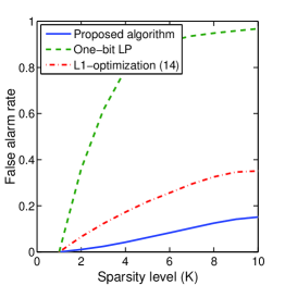
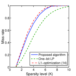
(a)	(b)

Figure 1: (a). False alarm rates of respective algorithms; (b). Miss rates of respective algorithms.

V Conclusions

We proposed an iterative reweighted algorithm for sparse signal reconstruction from one-bit quantized measurements. The proposed algorithm consists of solving a sequence of minimization problems whose weights are updated based on the current estimate. Analyses and simulation results show that the proposed algorithm that uses the log-sum penalty function is more sparsity-encouraging than $l_{1}$-based methods, and outperforms $l_{1}$ type methods in recovering the true support of the sparse signal.

References

- [1] E. Candés and T. Tao, “Decoding by linear programming,” IEEE Trans. Information Theory, no. 12, pp. 4203–4215, Dec. 2005.
- [2] J. A. Tropp and A. C. Gilbert, “Signal recovery from random measurements via orthogonal matching pursuit,” IEEE Trans. Information Theory, vol. 53, no. 12, pp. 4655–4666, Dec. 2007.
- [3] M. J. Wainwright, “Information-theoretic limits on sparsity recovery in the high-dimensional and noisy setting,” IEEE Trans. Information Theory, vol. 55, no. 12, pp. 5728–5741, Dec. 2009.
- [4] L. Jacques, J. N. Laska, P. T. Boufounos, and R. G. Baraniuk, “Robust 1-bit compressive sensing via binary stable embeddings of sparse vectors,” Apr. 2011 [online]. Available: http://arxiv.org/abs/1104.3160.
- [5] Y. Plan and R. Vershynin, “One-bit compressed sensing by linear programming,” Sep. 2011 [online]. Available: http://arxiv.org/abs/1109.4299.
- [6] T. Wimalajeewa and P. K. Varshney, “Performance bounds for sparsity pattern recovery with quantized noisy random projections,” IEEE Journal on Selected Topics in Signal Processing, vol. 6, no. 1, pp. 43–57, Feb. 2012.
- [7] P. T. Boufounos and R. G. Baraniuk, “One-bit compressive sensing,” in Proceedings of the 42nd Annual Conference on Information Sciences and Systems (CISS 08), Princeton, NJ, 2008.
- [8] J. N. Laska and R. G. Baraniuk, “Regime change: bit-depth versus measurement-rate in compressive sensing,” IEEE Trans. Signal Processing, vol. 60, no. 7, pp. 3496–3505, July 2012.
- [9] P. T. Boufounos, “Greedy sparse signal reconstruction from sign measurements,” in Proceedings of the 43rd Asilomar Conference on Signals, Systems, and Computers (Asilomar 09), Pacific Grove, California, 2009.
- [10] J. N. Laska, Z. Wen, W. Yin, and R. G. Baraniuk, “Trust, but verify: fast and accurate signal recovery from 1-bit compressive measurements,” IEEE Trans. Signal Processing, vol. 59, no. 11, pp. 5289–5301, Nov. 2011.
- [11] M. Yan, Y. Yang, and S. Osher, “Robust 1-bit compressive sensing using adaptive outlier pursuit,” IEEE Trans. Signal Processing, vol. 60, no. 7, pp. 3868–3875, July 2012.
- [12] R. R. Coifman and M. Wickerhauser, “Entropy-based algorithms for best basis selction,” IEEE Trans. Inform. Theory, vol. IT-38, pp. 713–718, Mar. 1992.
- [13] B. D. Rao and K. Kreutz-Delgado, “An affine scaling methodology for best basis selection,” IEEE Trans. Signal Processing, vol. 47, no. 1, pp. 187–200, Jan. 1999.
- [14] K. Lange, D.Hunter, and I. Yang, “Optimization transfer using surrogate objective functions,” Computational and Graphical Statistics, vol. 9, pp. 1–59, 2000.
- [15] I. F. Gorodnitsky and B. D. Rao, “Sparse signal reconstructions from limited data using focuss: A re-weighted minimum norm algorithm,” IEEE Trans. Signal Processing, vol. 45, no. 3, pp. 699–616, Mar. 1997.
- [16] E. J. Candes, M. B. Wakin, and S. P. Boyd, “Enhancing sparsity by reweighted minimization,” Journal of Fourier Analysis and Applications, vol. 14, pp. 877–905, Dec. 2008.