Underapproximation of Procedure Summaries for Integer Programs

Abstract

We show how to underapproximate the procedure summaries of recursive programs over the integers using off-the-shelf analyzers for non-recursive programs. The novelty of our approach is that the non-recursive program we compute may capture unboundedly many behaviors of the original recursive program for which stack usage cannot be bounded. Moreover, we identify a class of recursive programs on which our method terminates and returns the precise summary relations without underapproximation. Doing so, we generalize a similar result for non-recursive programs to the recursive case. Finally, we present experimental results of an implementation of our method applied on a number of examples.

1 Introduction

Formal approaches to reasoning about behaviors of programs usually fall into one of the following two categories: certification approaches, that provide proofs of correctness, and bug-finding approaches, that explore increasingly larger sets of traces in order to find possible errors. While the methods in the first category are used typically in the development of safety-critical software whose failures may incur dramatic losses in terms of human lives (airplanes, space missions, or nuclear power plants), the methods in the second category have a broad application in industry, outside of the safety-critical market niche. Another difference between the two categories is methodological: certification approaches are based on over-approximations of the set of behaviors (if the over-approximation is free of errors, the original system is correct), while bug-finding needs systematic under-approximation techniques (if there are errors, the method will eventually discover all of them). Finally, over-approximation methods are guaranteed to terminate, but the answer might be inconclusive (spurious errors are introduced due to the abstraction), whereas under-approximation methods provide precise results (all reported errors are real), but with no guarantee for termination.

Procedure summaries are relations between the input and return values of a procedure, resulting from its terminating executions. Computing summaries is important, as they are a key enabler for the development of modular verification techniques for inter-procedural programs, such as checking safety, termination or equivalence properties. Summary computation is, however, challenging in the presence of recursive procedures with integer parameters, return values, and local variables. While many analysis tools exist for non-recursive programs, only a few ones address the problem of recursion (e.g. InterProc [19]).

In this paper, we propose a novel technique to generate arbitrarily precise underapproximations of summary relations. Our technique is based on the following idea. The control flow of procedural programs is captured precisely by the language of a context-free grammar. A $k$-index underapproximation of this language (where $k\geq 1$) is obtained by filtering out those derivations of the grammar that exceed a budget, called index, on the number (at most $k$) of occurrences of nonterminals occurring at each derivation step. As expected, the higher the index, the more complete the coverage of the underapproximation. From there we define the $k$-index summary relations of a program by considering the $k$-index underapproximation of its control flow. Our method then reduces the computation of $k$-index summary relations for a recursive program to the computation of summary relations for a non-recursive program, which is, in general, easier to compute because of the absence of recursion. The reduction was inspired by a decidability proof [4] in the context of Petri nets.

The contributions of this paper are threefold. First, we show that, for a given index, recursive programs can be analyzed using off-the-shelf analyzers designed for non-recursive programs. Second, we identify a class of recursive programs, with possibly unbounded stack usage, on which our technique is complete, i.e. it terminates and returns the precise result. Third, we present experimental results of an implementation of our method applied on a number of examples.

Motivating Example To properly introduce the reader to our result, we describe our source-to-source program transformation through an illustrative example. Consider the recursive program $\mathcal{P}={\left\{P\right\}}$, consisting of a single recursive procedure $P$, given in Fig. 1 (a), whose control flow graph is given in Fig. 1 (b). The nodes of this graph represent control locations in the program, with a designated initial location $Q^{init}_{1}$ and a final location $\varepsilon$. The edges are labeled with relations denoting the program semantics, where primed variables $x^{\prime}$ and $z^{\prime}$ denote the values at the next step. For instance, the edge $t_{2}:Q_{2}\xrightarrow[\scriptstyle]{{\scriptstyle z^{\prime}=P(x-1)\wedge x^{\prime}=x}}Q_{3}$ corresponds to the recursive call on line $3$ in the program—the edge labels of the control flow graph explicitly mention the copies of variables not changed by the program action corresponding to the edge, e.g. $x^{\prime}=x$.

In this paper, we model programs using visibly pushdown grammars (VPG) [3]. The VPG for $P$ is given in Fig. 1 (c). The role of the grammar is to define the set of interprocedurally valid paths in the control-flow graph of the program $P$. Every edge in the control-flow graph matches one or two symbols from the finite alphabet ${\left\{\tau_{1},\langle\!\!\langle\tau_{2},\tau_{2}\rangle\!\!\rangle,\tau_{3},\tau_{4}\right\}}$, where $\langle\!\!\langle\tau_{2}$ and $\tau_{2}\rangle\!\!\rangle$ denote the call and return, respectively. Each edge in the graph translates to a production rule in the grammar, labeled $p^{b}_{1},p^{c}_{2},p^{a}_{3}$ and $p^{a}_{4}$—the superscript $a$, $b$ and $c$ distinguishes rules with $0$, $1$ and $2$ nonterminals on the right-hand side, respectively. For instance, the call edge $t_{2}$ becomes the rule $Q_{2}\rightarrow\langle\!\!\langle\tau_{2}Q^{init}_{1}\tau_{2}\rangle\!\!\rangle Q_{3}$. The language of the grammar of Fig. 1 (c) (with axiom $Q^{init}_{1}$) is the set ${\left\{\left(\tau_{1}\langle\!\!\langle\tau_{2}\right)^{n}\tau_{4}\left(\tau_{2}\rangle\!\!\rangle\tau_{3}\right)^{n}\mid n\in{\bf\mathbb{N}}\right\}}$ of interprocedurally valid paths, where each call symbol $\langle\!\!\langle\tau_{2}$ is matched by a return symbol $\tau_{2}\rangle\!\!\rangle$, and the matching relation is well-parenthesized.

The outcome of the program transformation applied to $P$ is the non-recursive program $\mathcal{Q}={\left\{\mathit{query}^{i}\right\}}_{i=0}^{K}$, depicted in Fig. 1 (d), where $K$ is a parameter of our analysis. The main idea is that the executions of the procedure $\mathit{query}^{k}$, ending with an empty stack, correspond to the derivations of the VPG in Fig. 1 (c), of index at most $k$—since there is no derivation of index $0$, the set of executions of $\mathit{query}^{0}$ will be empty. The body of a procedure $\mathit{query}^{k}$ consists of a main loop, starting at the control label $begin\_loop$ in Fig. 1 (d). Each branch inside the main loop corresponds to the simulation of one of the production rules of the grammar in Fig. 1 (c) and starts with a control label which is the name of that rule ($p_{1}^{b},p_{2}^{c},p_{3}^{a},p_{4}^{a}$). Next, we explain the relations labeling the control edges of $\mathit{query}^{k}$. For each production rule $p$ in the grammar we have a relation $\rho_{p}(x_{I},z_{I},x_{O},z_{O})$, where subscript $I$ and $O$ denote the input and output copies of the program variables of $P$, respectively. In addition, we consider auxiliary copies $x_{J},z_{J}$, $x_{K},z_{K}$ and $x_{L},z_{L}$, defined in a similar way. For instance, the auxiliary variables store intermediate results of the computation of $p^{c}_{2}$ as follows: $[x_{I},z_{I}]\;\langle\!\!\langle\tau_{2}\;[x_{J},z_{J}]\;Q^{init}_{1}\;[x_{K},z_{K}]\;\tau_{2}\rangle\!\!\rangle\;[x_{L},z_{L}]\;Q_{3}\;[x_{O},z_{O}]$. The transition $p_{2}^{c}\rightarrow in\_order/out\_of\_order$ can be understood by noticing that $\langle\!\!\langle\tau_{2}$ gives rise to the constraint $x_{J}=x_{I}-1$, $\tau_{2}\rangle\!\!\rangle$ to $z_{L}=z_{K}$ and $x_{I}=x_{L}$ corresponds to the frame condition $x^{\prime}=x$.

The peculiarity of the resulting program is that a function call is modeled in two possible ways: (i) in-orderexecution of the function body, followed by the continuation of the call, and (ii) out-of-orderexecution of the continuation, followed by the execution of the function body. The two cases correspond to $k$-index derivations of the VPG in Fig 1 (c) of the form $uQ_{1}^{init}vQ_{3}w\Rightarrow^{*}uv_{1}vQ_{3}w\Rightarrow^{*}uv_{1}vv_{2}w$ and $uQ_{1}^{init}vv_{2}w\Rightarrow^{*}uv_{1}vv_{2}w\Rightarrow^{*}uv_{1}vv_{2}w$, respectively, where $Q_{1}^{init}\Rightarrow^{*}v_{1}$ and $Q_{3}\Rightarrow^{*}v_{2}$ are derivations of the VPG. In the first case, the control path simulating the derivation in $\mathit{query}^{k}$ follows the left branch $in\_order/out\_of\_order\rightarrow begin\_loop$, whereas the second case is simulated by the right branch.

Since the only call of $query^{k}$ is to $query^{k-1}$, on the edges $in\_order/out\_of\_order\rightarrow begin\_loop$, the whole program is a non-recursive under-approximation of the semantics of the original program $P$, amenable to analysis using intra-procedural program analysis tools. Indeed, the computation of the pre-condition relation of the program $\mathcal{Q}=\{\mathit{query}^{2},\mathit{query}^{1}$, $\mathit{query}^{0}\}$ with the Flata tool [17] yields the formula $z_{O}=2\cdot x_{I}$, which matches the summary $z^{\prime}=2\cdot x$ of the program $P$.

In other words, the analysis of the under-approximation of $\mathcal{P}$ of index at most $2$ suffices to infer the complete summary of the program (the analysis for values $K>2$ will necessarily yield the same result, since the under-approximation method is monotonic in $K$). This fact matches the completeness result of Section 5, stating that the analysis needs to be carried up to a certain bound (linear in the size of the program’s VPG) whenever the language of the VPG is included in the language of the regular expression $w_{1}^{*}\ldots w_{n}^{*}$, for some non-empty words $w_{1},\ldots,w_{n}$. In our case, the completeness result applies due to ${\left\{\left(\tau_{1}\langle\!\!\langle\tau_{2}\right)^{n}\tau_{4}\left(\tau_{2}\rangle\!\!\rangle\tau_{3}\right)^{n}\mid n\in{\bf\mathbb{N}}\right\}}\subseteq\left(\tau_{1}\langle\!\!\langle\tau_{2}\right)^{*}\tau_{4}^{*}\left(\tau_{2}\rangle\!\!\rangle\tau_{3}\right)^{*}$.

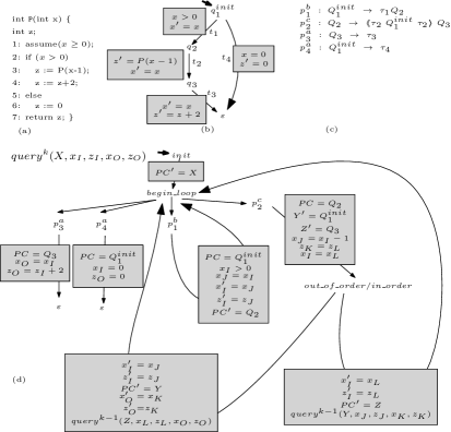
Figure 1: A recursive program returning the parameter value multiplied by two (a), its corresponding control flow graph (b) and visibly pushdown grammar (c), and the non-recursive program $query^{k}(X,x_{I},z_{I},x_{O},z_{O})$ resulting from our index-bounded under-approximation (d).

Related Work The problem of analyzing recursive programs handling integers (in general, unbounded data domains) has gained significant interest with the seminal work of Sharir and Pnueli [24]. They proposed two orthogonal approaches for interprocedural dataflow analysis. The first one keeps precise values (call strings) up to a limited depth of the recursion stack, which bounds the number of executions. In contrast to the methods based on the call strings approach, our method can also analyse precisely certain programs for which the stack is unbounded, allowing for unbounded number of executions to be represented at once.

The second approach of Sharir and Pnueli [24] is based on computing the least fixed point of a system of recursive dataflow equations (the functional approach). This approach to interprocedural analysis is based on computing an increasing Kleene sequence of abstract summaries. It is to be noticed that abstraction is key to ensuring termination of the Kleene sequence, the result being an over-approximation of the precise summary. Recently [11], a Newton sequence defined over the language semiring was shown to converge at least as fast as the Kleene sequence over the same semiring. An iterate of a Newton sequence is the set of control paths in the program that correspond to words produced by a grammar, with bounded number of nonterminals at each step in the derivation. By increasing this bound, we obtain an increasing sequence of languages that converges to the language of behavior of the program. Our contribution can be thus seen as a technique to compute the iterates of the Newton sequence for programs with integer parameters, return values, and local variables, the result being, at each step, an under-approximation of the precise summary.

The complexity of the functional approach was shown to be polynomial in the size of the (finite) abstract domain, in the work of Reps, Horwitz and Sagiv [23]. This result is achieved by computing summary information, in order to reuse previously computed information during the analysis. Following up on this line of work, most existing abstract analyzers, such as InterProc [19], also use relational domains to compute over-approximations of function summaries – typically widening operators are used to ensure termination of fixed point computations. The main difference of our method with respect to static analyses is the use of under-approximation instead of over-approximation. If the final purpose of the analysis is program verification, our method will not return false positives. Moreover, the coverage can be increased by increasing the bound on the derivation index.

Previous works have applied model checking based on abstraction refinement to recursive programs. One such method, known as nested interpolants represents programs as nested word automata [3], which have the same expressive power as the visibly pushdown grammars used in our paper. Also based on interpolation is the Whale algorithm [2], which combines partial exploration of the execution paths (underapproximation) with the overapproximation provided by a predicate-based abstract post operator, in order to compute summaries that are sufficient to prove a given safety property. Another technique, similar to Whale, although not handling recursion, is the Smash algorithm [15] which combines may- and must-summaries for compositional verification of safety properties. These approaches are, however, different in spirit from ours, as their goal is proving given safety properties of programs, as opposed to computing the summaries of procedures independently of their calling context, which is our case. We argue that summary computation can be applied beyond safety checking, e.g., to prove termination [5], or program equivalence.

The technique of under-approximation is typically used for bug discovery, rather than certification of correctness. For instance, bug detection based on under-approximation has been developed for non-recursive C programs with arrays [18]. Our approach in orthogonal, as we consider more complex control structures (possibly recursive procedure calls) but simpler data domains (scalar values such as integers).

Paper organization. After introducing the basic definition in Section 2, we present, in Section 3, our model for programs, a semantics based on nested words and another one, equivalent, based on derivations of the underlying grammar. Then, in Section 4, we present our main contribution which is a program transformation underapproximating the semantics of the input program. In Section 5, we define a class of programs for which the underapproximation is complete. Finally, after reporting on experiments in Section 6 we conclude in Section 7.

2 Preliminaries

2.1 Grammars

Let $\Sigma$ be an alphabet, that is a finite non-empty set of symbols. We denote by $\Sigma^{*}$ the set of finite words over $\Sigma$ including $\varepsilon$, the empty word. Given a word $w\in\Sigma^{*}$, let $|w|$ denote its length and let $(w)_{i}$, with $1\leq i\leq|w|$, be the $i$-th symbol of $w$. By $(w)_{i\ldots j}$, with $1\leq i\leq j\leq|w|$, we denote the subword $(w)_{i}\ldots(w)_{j}$ of $w$. For a word $w\in\Sigma^{*}$ and $\Sigma^{\prime}\subseteq\Sigma$, we denote by $w\mathbin{\downarrow}_{\Sigma^{\prime}}$ the result of erasing all symbols of $w$ not in $\Sigma^{\prime}$.

A context-free grammar (or simply grammar) is a tuple $G={\langle\Xi,\Sigma,\Delta\rangle}$, where $\Xi$ is a finite nonempty set of nonterminals, $\Sigma$ is an alphabet, such that $\Xi\cap\Sigma=\emptyset$, and $\Delta\subseteq\Xi\times(\Sigma\cup\Xi)^{*}$ is a finite set of productions. A production $(X,w)\in\Delta$ is often conveniently noted $X\rightarrow w$. Also define $\mathit{head(X\rightarrow w)=X}$ and $\mathit{tail}(X\rightarrow w)=w$. Given two strings $u,v\in(\Sigma\cup\Xi)^{*}$, a production $(X,w)\in\Delta$ and $1\leq j\leq|u|$, we define a step $u\xRightarrow{(X,w)/j}_{G}v$ if, and only if, $(u)_{j}=X$ and $v=(u)_{1}\cdots(u)_{j-1}\cdot w\cdot(u)_{j+1}\cdots(u)_{|u|}$. We omit $(X,w)$ or $j$ above the arrow when it is not important. In this notation and others, when $G$ is clear from the context, we omit it. Step sequences (including the empty sequence) are defined using the reflexive transitive closure of the step relation $\xRightarrow{}_{G}$, denoted $\xRightarrow{}^{*}_{G}$. For instance, $X\xRightarrow{}^{*}_{G}w$ means there exists a sequence of steps that produces the word $w\in(\Sigma\cup\Xi)^{*}$, starting from $X$. We call any step sequence $v\xRightarrow{}^{*}_{G}w$ a derivation whenever $v\in\Xi$ and $w\in\Sigma^{*}$. The language produced by $G$, starting with a nonterminal $X$ is the set $L_{X}(G)={\left\{w\in\Sigma^{*}\mid X\xRightarrow{}^{*}_{G}w\right\}}$.

By defining a control word to be a sequence of productions $\gamma\in\Delta^{*}$, we can annotate step sequences as expected: $\varepsilon\in\Delta^{*}$ is the control word for empty step sequences, and given a control word $\gamma$ of length $n$ we write $u\xRightarrow{\gamma}_{G}v$ whenever there exists $w_{0},\ldots,w_{n}\in(\Xi\cup\Sigma)^{*}$ such that

$$u=w_{0}\xRightarrow{(\gamma)_{1}}_{G}w_{1}\xRightarrow{(\gamma)_{2}}_{G}\ldots w_{n-1}\xRightarrow{(\gamma)_{n}}_{G}w_{n}=v\enspace.$$

Given a nonterminal $X\in\Xi$ and a set $\Gamma\subseteq\Delta^{*}$ of control words (a.k.a control set), we denote by $\hat{L}_{X}(\Gamma,G)=\{w\in\Sigma^{*}\mid\exists\gamma\in\Gamma\colon X\xRightarrow{\gamma}w\}$ the language generated by $G$ using only control words in $\Gamma$.

2.2 Visibly Pushdown Grammars

To model the control flow of procedural programs we use languages generated by visibly pushdown grammars, a subset of context-free grammars. In this setting, words are defined over a tagged alphabet $\widehat{\Sigma}=\Sigma\cup\langle\!\!\langle\Sigma\cup\Sigma\rangle\!\!\rangle$, where $\langle\!\!\langle\Sigma=\{\langle\!\!\langle a\mid a\in\Sigma\}$ represents procedure call sites and $\Sigma\rangle\!\!\rangle=\{a\rangle\!\!\rangle\mid a\in\Sigma\}$ represents procedure return sites. Formally, a visibly pushdown grammar $G={\langle\Xi,\widehat{\Sigma},\Delta\rangle}$ is a grammar that has only productions of the following forms, for some $a,b\in\Sigma$:

$$X \rightarrow a X \rightarrow a\,Y X \rightarrow\langle\!\!\langle a\,Y\,b\rangle\!\!\rangle\,Z\enspace.$$

It is worth pointing that, for our purposes, we do not need a visibly pushdown grammar to generate the empty string $\varepsilon$. Each tagged word generated by visibly pushdown grammars is associated a nested word [3] the definition of which we briefly recall. Given a finite alphabet $\Sigma$, a nested word over $\Sigma$ is a pair $(w,\leadsto)$, where $\mathord{\leadsto}\subseteq\{1,\ldots,{|{w}|}\}\times\{1,\ldots,{|{w}|}\}$ is a set of nesting edges (or simply edges) where:

1. $i\leadsto j$ only if $i<j$; edges only go forward;

2. ${|\!|{\{j\mid i\leadsto j\}}|\!|}\leq 1$ and ${|\!|{\{i\mid i\leadsto j\}}|\!|}\leq 1$; no two edges share a call/return position;

3. if $i\leadsto j$ and $k\leadsto\ell$ then it is not the case that $i<k\leq j<\ell$; edges do not cross.

Intuitively, we associate a nested word to a tagged word as follows: there is an edge between tagged symbols $\langle\!\!\langle a$ and $b\rangle\!\!\rangle$ if and only if both symbols are produced by the same derivation step. Finally, let $w\_nw$ denote the mapping which given a tagged word in the language of a visibly pushdown grammar returns the nested word thereof.

Example 2.1.

For the tagged word $w=\tau_{1}\langle\!\!\langle\tau_{2}\tau_{1}\langle\!\!\langle\tau_{2}\tau_{4}\tau_{2}\rangle\!\!\rangle\tau_{3}\tau_{2}\rangle\!\!\rangle\tau_{3}$, $w\_nw(w)=(\tau_{1}\tau_{2}\tau_{1}\tau_{2}\tau_{4}\tau_{2}\tau_{3}\tau_{2}\tau_{3},{\left\{2\leadsto 8,4\leadsto 6\right\}})$ is the associated nested word. $\blacksquare$

2.3 Integer Relations

Given a set $S$, let ${|\!|{S}|\!|}$ denote its cardinality. We denote by $\mathbb{Z}$ the set of integers. Let ${\mathbf{x}}={\langle x_{1},\ldots,x_{d}\rangle}$ be a tuple of variables, for some $d>0$. We define by ${\mathbf{x}}^{\prime}$ the primed variables of ${\mathbf{x}}$ to be the tuple ${\langle x^{\prime}_{1},x^{\prime}_{2},\ldots,x^{\prime}_{d}\rangle}$. We consider implicitly that all variables range over $\mathbb{Z}$. We denote by ${|{{\mathbf{x}}}|}=d$ the length of the tuple ${\mathbf{x}}$, and for a tuple ${\mathbf{y}}={\langle y_{1},\ldots,y_{e}\rangle}$, we denote by ${\mathbf{x}}\cdot{\mathbf{y}}={\langle x_{1},\ldots,x_{d},y_{1},\ldots,y_{e}\rangle}$ their concatenation. For two tuples of variables ${\mathbf{t}}$ and ${\mathbf{s}}$ such that ${|{t}|}={|{s}|}=k$, we denote by ${\mathbf{t}}={\mathbf{s}}$ the conjunction $\bigwedge_{i=1}^{k}t_{i}=s_{i}$.

A linear term $t$ is a linear combination of the form $a_{0}+\sum_{i=1}^{d}a_{i}x_{i}$, where $a_{0},\ldots,a_{d}\in\mathbb{Z}$. An atomic proposition is a predicate of the form $t\leq 0$, where $t$ is a linear term. We consider formulae in the first-order logic over atomic propositions $t\leq 0$, also known as Presburger arithmetic. A valuation of ${\mathbf{x}}$ is a function $\smash{\nu:{\mathbf{x}}\xrightarrow[\scriptstyle]{{\scriptstyle}}\mathbb{Z}}$. The set of all valuations of ${\mathbf{x}}$ is denoted by $\mathbb{Z}^{{\mathbf{x}}}$. If ${\mathbf{x}}={\langle x_{1},\ldots,x_{d}\rangle}$ and $\nu\in\mathbb{Z}^{{\mathbf{x}}}$, then $\nu({\mathbf{x}})$ denotes the tuple ${\langle\nu(x_{1}),\ldots,\nu(x_{d})\rangle}$. An arithmetic formula $\mathcal{R}({\mathbf{x}},{\mathbf{y}}^{\prime})$ defining a relation $R\subseteq\mathbb{Z}^{{\mathbf{x}}}\times\mathbb{Z}^{{\mathbf{y}}}$ is evaluated with respect to two valuations $\nu_{1}\in\mathbb{Z}^{{\mathbf{x}}}$ and $\nu_{2}\in\mathbb{Z}^{{\mathbf{y}}}$, by replacing each $x\in{\mathbf{x}}$ by $\nu_{1}(x)$ and each $y^{\prime}\in{\mathbf{y}}^{\prime}$ by $\nu_{2}(y)$ in $\mathcal{R}$. The composition of two relations $R_{1}\subseteq\mathbb{Z}^{{\mathbf{x}}}\times\mathbb{Z}^{{\mathbf{y}}}$ and $R_{2}\subseteq\mathbb{Z}^{{\mathbf{y}}}\times\mathbb{Z}^{{\mathbf{z}}}$ is denoted by $R_{1}\comp R_{2}=\{{\langle{\mathbf{u}},{\mathbf{v}}\rangle}\in\mathbb{Z}^{{\mathbf{x}}}\times\mathbb{Z}^{{\mathbf{z}}}\mid\exists{\mathbf{t}}\in\mathbb{Z}^{{\mathbf{y}}}\ldotp{\langle{\mathbf{u}},{\mathbf{t}}\rangle}\in R_{1}~{}\mbox{and}~{}{\langle{\mathbf{t}},{\mathbf{v}}\rangle}\in R_{2}\}$. We denote ${\mathbf{y}}\subseteq{\mathbf{x}}$ if ${\mathbf{y}}={\langle x_{i_{1}},\ldots,x_{i_{\ell}}\rangle}$, for a sequence of indices $1\leq i_{1}<\ldots<i_{\ell}\leq d$ of ${\mathbf{x}}$. For a valuation $\nu\in\mathbb{Z}^{{\mathbf{x}}}$ and a tuple ${\mathbf{y}}\subseteq{\mathbf{x}}$, we denote by $\nu\mathbin{\downarrow}_{\mathbf{y}}\in\mathbb{Z}^{{\mathbf{y}}}$ the projection of $\nu$ onto variables ${\mathbf{y}}$, i.e. $\nu\mathbin{\downarrow}_{\langle y_{1},\ldots,y_{k}\rangle}={\langle\nu(y_{1}),\ldots,\nu(y_{k})\rangle}$. Finally, given two valuations $I,O\in\mathbb{Z}^{{\mathbf{x}}}$, we denote by $I\cdot O$ the valuation $I({\mathbf{x}})\cdot O({\mathbf{x}})$, and we define $\mathbb{Z}^{{\mathbf{x}}\times{\mathbf{x}}}=\{I\cdot O~{}|~{}I,O\in\mathbb{Z}^{\mathbf{x}}\}$.

2.4 Parikh Images

Let $\Theta=\{\theta_{1},\ldots,\theta_{k}\}$ be a linearly ordered subset of the alphabet $\Sigma$. For a symbol $a\in\Sigma$ its Parikh image is defined as $Pk_{\Theta}(a)={\mathbf{e}}_{i}$ if $a=\theta_{i}$, where ${\mathbf{e}}_{i}$ is the $k$-dimensional vector having $1$ on the $i$-th position and $0$ everywhere else. Otherwise, if $a\in\Sigma\setminus\Theta$, let $Pk_{\Theta}(a)={\mathbf{0}}$ where ${\mathbf{0}}$ is the $k$-dimensional vector with $0$ everywhere. For a word $w\in\Sigma^{*}$ of length $n$, we define $Pk_{\Theta}(w)=\sum_{i=1}^{n}Pk_{\Theta}((w)_{i})$. Furthermore, let $Pk_{\Theta}(L)=\{Pk_{\Theta}(w)\mid w\in L\}$ for any language $L\subseteq\Sigma^{*}$.

2.5 Labelled Graphs

In this paper we use of the notion of labelled graph $\mathcal{G}={\langle Q,\mathcal{L},\delta\rangle}$, where $Q$ is a finite set of vertices, $\mathcal{L}$ is a set of labels whose elements label edges as defined by the edge relation $\delta\subseteq Q\times S\times Q$. We denote by $q\xrightarrow[\scriptstyle]{{\scriptstyle\ell}}q^{\prime}$ the fact that $(q,\ell,q^{\prime})\in\delta$. A path $\pi$ in $\mathcal{G}$ is an alternating sequence of vertices and edges whose endpoints are vertices. Sometimes, $\pi$ is conveniently written as $q_{0}\xrightarrow[\scriptstyle]{{\scriptstyle\ell_{1}}}q_{1}\xrightarrow[\scriptstyle]{{\scriptstyle\ell_{2}}}\ldots q_{n-1}\xrightarrow[\scriptstyle]{{\scriptstyle\ell_{n}}}q_{n}$ and further abbreviated $q_{0}\xrightarrow[\scriptstyle]{{\scriptstyle w}}q_{n}$ where $w=\ell_{1}\ldots\ell_{n}$.

3 Integer Recursive Programs

We consider in the following that programs are collections of procedures calling each other, possibly according to recursive schemes. Formally, an integer program is an indexed tuple $\mathcal{P}=\langle P_{1},\ldots,P_{n}\rangle$, where $P_{1},\ldots,P_{n}$ are procedures. Each procedure is a tuple $P_{i}=\langle{\mathbf{x}}_{i},{\mathbf{x}}^{in}_{i},{\mathbf{x}}^{out}_{i},S_{i},q^{\mathit{init}}_{i},F_{i},\Delta_{i}\rangle$, where ${\mathbf{x}}_{i}$ are the local variables of $P_{i}$ (${\mathbf{x}}_{i}\cap{\mathbf{x}}_{j}=\emptyset$ for all $i\neq j$), ${\mathbf{x}}^{in}_{i},{\mathbf{x}}^{out}_{i}\subseteq{\mathbf{x}}_{i}$ are the tuples of input and output variables, $S_{i}$ are the control states of $P_{i}$ ($S_{i}\cap S_{j}=\emptyset$, for all $i\neq j$), $q^{\mathit{init}}_{i}\in S_{i}\setminus F_{i}$ is the initial, and $F_{i}\subseteq S_{i}$ ($F_{i}\neq\emptyset$) are the final states of $P_{i}$, and $\Delta_{i}$ is a set of transitions of one of the following forms:

• $q\xrightarrow[\scriptstyle]{{\scriptstyle\mathcal{R}({\mathbf{x}}_{i},{\mathbf{x}}^{\prime}_{i})}}q^{\prime}$ is an internal transition, where $q,q^{\prime}\in S_{i}$, and $\mathcal{R}({\mathbf{x}}_{i},{\mathbf{x}}^{\prime}_{i})$ is a Presburger arithmetic relation involving only the local variables of $P_{i}$;

• $q\xrightarrow[\scriptstyle]{{\scriptstyle{\mathbf{z}}^{\prime}=P_{j}({\mathbf{u}})}}q^{\prime}$ is a call, where $q,q^{\prime}\in S_{i}$, $P_{j}$ is the callee, ${\mathbf{u}}$ are linear terms over ${\mathbf{x}}_{i}$, ${\mathbf{z}}\subseteq{\mathbf{x}}_{i}$ are variables, such that ${|{{\mathbf{u}}}|}={|{{\mathbf{x}}^{in}_{j}}|}$ and ${|{{\mathbf{z}}}|}={|{{\mathbf{x}}^{out}_{j}}|}$. The call is said to be terminal if $q^{\prime}\in F_{i}$. It is well-known that terminal calls can be replaced by internal transitions.

The call graph of a program $\mathcal{P}=\langle P_{1},\ldots,P_{n}\rangle$ is a directed graph with vertices $P_{1},\ldots,P_{n}$ and an edge $(P_{i},P_{j})$, for each $P_{i}$ and $P_{j}$, such that $P_{i}$ has a call to $P_{j}$. A program is recursive if its call graph has at least one cycle, and non-recursive if its call graph is a dag.

In the rest of this paper, we denote by $\mathop{\mathcal{F}}(\mathcal{P})=\bigcup_{i=1}^{n}F_{i}$ the set of final states of the program $\mathcal{P}$, by $\mathop{n\!\mathcal{F}}(P_{i})$ the set $S_{i}\setminus F_{i}$ of non-final states of $P_{i}$, and by $\mathop{n\!\mathcal{F}}(\mathcal{P})=\bigcup_{i=1}^{n}\mathop{n\!\mathcal{F}}(\mathcal{P})$ be the set of non-final states of $\mathcal{P}$.

3.1 Simplified syntax

To ease the description of programs defined in this paper, we use a simplified, human readable, imperative language such that each procedure of the program conforms to the following grammar:

$$P ::=\mathbf{proc}\ P_{i}(\mathit{id}^{*})~{}\mathbf{begin}~{}\mathbf{var}~{}\mathit{id}^{*}~{}S_{0};\,S~{}\mathbf{end}$$

$$\begin{split}S_{0}&::=\mathbf{assume}\ f\mid\mathbf{goto}\ \ell^{+}\mid\mathbf{havoc}\ \mathit{id}^{+}\mid id\leftarrow t\\ S&::=S_{0}\mid S;\,S\mid id\leftarrow P_{i}(t^{*});\,S_{0}\mid P_{i}(t^{*});\,S_{0}\mid\mathbf{return}\ \mathit{id}\end{split}$$

The local variables occurring in $P$ are denoted by $id$, linear terms by $t$, Presburger formulae by $f$, and control labels by $\ell$. Each procedure consists in local declarations followed by a sequence of statements. Statements may carry a label. Program statements can be either assume statements, assignments, procedure calls (possibly with a return value), return to the caller (possibly with a value), non-deterministic jumps goto $\ell_{1}~{}\mbox{\bf or}~{}\ldots~{}\mbox{\bf or}~{}\ell_{n}$, and havoc $x_{1},x_{2},\ldots,x_{n}$ statements. In order to simplify the upcoming technical developments, we forbid empty procedures, procedures starting with a call or a return, i.e. each procedure must start with a statement generated by the $S_{0}$ nonterminal. We consider the usual syntactic requirements (used variables must be declared, jumps are well defined, no jumps outside procedures, etc.). We do not define them, it suffices to know that all simplified programs in this paper comply with the requirements. A program using the simplified syntax can be easily translated into the formal syntax (Fig. 1).

Example 3.1.

Figure 1 shows a program in our simplified imperative language and its corresponding integer program $\mathcal{P}$. Formally, $\mathcal{P}=\langle P\rangle$, where $P$ is the only procedure in the program, defined as:

$$P=\langle\{x,z\},\{x\},\{z\},\{q_{1}^{\mathit{init}},q_{2},q_{3},\varepsilon\},q_{1}^{\mathit{init}},\{\varepsilon\},\{t_{1},t_{2},t_{3},t_{4}\}\rangle$$

Since $P$ calls itself once (within the call transition $t_{2}$), this program is recursive. $\blacksquare$

3.2 Semantics

We are interested in computing the summary relation between the values of the input and output variables of a procedure. To this end, we give the semantics of a program $\mathcal{P}=\langle P_{1},\ldots,P_{n}\rangle$ as a tuple of relations, denoted $\llbracket q\rrbracket$ in the following, describing, for each non-final control state $q\in\mathop{n\!\mathcal{F}}(P_{i})$ of a procedure $P_{i}$, the effect of the program when started in $q$ upon reaching a state in $F_{i}$. The summary of a procedure $P_{i}$ is the relation corresponding to its unique initial state, i.e. $\llbracket q_{i}^{\mathit{init}}\rrbracket$.

An interprocedurally valid path is represented by a tagged word over an alphabet $\widehat{\Theta}$, which maps each internal transition $t$ to a symbol $\tau$, and each call transition $t$ to a pair of symbols $\langle\!\!\langle\tau,\tau\rangle\!\!\rangle\in\widehat{\Theta}$. In the sequel, we denote by $Q$ the nonterminal corresponding to the control state $q$, and by $\tau\in\Theta$ the alphabet symbol corresponding to the transition $t$ of $\mathcal{P}$. Formally, we associate $\mathcal{P}$ a visibly pushdown grammar, denoted in the rest of the paper by $G_{\mathcal{P}}={\langle\Xi,\widehat{\Theta},\Delta\rangle}$, such that $Q\in\Xi$ if and only if $q\in\mathop{n\!\mathcal{F}}(\mathcal{P})$ and:

• $Q\rightarrow\tau\in\Delta$ if and only if $t\colon q\xrightarrow[\scriptstyle]{{\scriptstyle\mathcal{R}}}q^{\prime}$ and $q^{\prime}\in\mathop{\mathcal{F}}(\mathcal{P})$

• $Q\rightarrow\tau~{}Q^{\prime}\in\Delta$ if and only if $t\colon q\xrightarrow[\scriptstyle]{{\scriptstyle\mathcal{R}}}q^{\prime}$ and $q^{\prime}\in\mathop{n\!\mathcal{F}}(\mathcal{P})$

• $Q\rightarrow\langle\!\!\langle\tau~{}Q_{j}^{\mathit{init}}~{}\tau\rangle\!\!\rangle~{}Q^{\prime}\in\Delta$ if and only if $t\colon q\xrightarrow[\scriptstyle]{{\scriptstyle{\mathbf{z}}^{\prime}=P_{j}({\mathbf{u}})}}q^{\prime}$.

It is easily seen that interprocedurally valid paths in $\mathcal{P}$ and tagged words in $G_{\mathcal{P}}$ are in one-to-one correspondence. In fact, each interprocedurally valid path of $\mathcal{P}$ between state $q\in\mathop{n\!\mathcal{F}}(P_{i})$ and a state of $F_{i}$, where $1\leq i\leq n$, corresponds exactly to one tagged word of $L_{Q}(G_{\mathcal{P}})$.

Example 3.2.

(contd. from Ex. 3.1) The visibly pushdown grammar $G_{\mathcal{P}}$ corresponding to $\mathcal{P}$ is given in Fig. 1 (c). In the following, we use superscripts $a,b,c$ to distinguish productions of the form ($a$) $Q\rightarrow\tau$, ($b$) $Q\rightarrow\tau\,Q^{\prime}$ or ($c$) $Q\rightarrow\langle\!\!\langle\tau\,Q_{j}^{\mathit{init}}\,\tau\rangle\!\!\rangle\,Q^{\prime}$, respectively. The language $L_{Q_{1}^{\mathit{init}}}(G_{\mathcal{P}})$ generated by $G_{\mathcal{P}}$ starting with $Q_{1}^{\mathit{init}}$ contains the word $w=\tau_{1}\langle\!\!\langle\tau_{2}\tau_{1}\langle\!\!\langle\tau_{2}\tau_{4}\tau_{2}\rangle\!\!\rangle\tau_{3}\tau_{2}\rangle\!\!\rangle\tau_{3}$, of which $w\_nw(w)=(\tau_{1}\tau_{2}\tau_{1}\tau_{2}\tau_{4}\tau_{2}\tau_{3}\tau_{2}\tau_{3},{\left\{2\leadsto 8,4\leadsto 6\right\}})$ is the corresponding nested word. The word $w$ corresponds to an interprocedurally valid path where $P$ calls itself twice. The control words $\gamma_{1}=p_{1}^{b}p_{2}^{c}p_{1}^{b}p_{2}^{c}p_{4}^{a}p_{3}^{a}p_{3}^{a}$ and $\gamma_{2}=p_{1}^{b}p_{2}^{c}p_{3}^{a}p_{1}^{b}p_{2}^{c}p_{4}^{a}p_{3}^{a}$ both produce $w$ in this case, i.e. $Q_{1}^{\mathit{init}}\stackrel{{\scriptstyle\gamma_{1}}}{{\Longrightarrow}}w$ and $Q_{1}^{\mathit{init}}\stackrel{{\scriptstyle\gamma_{2}}}{{\Longrightarrow}}w$. $\blacksquare$

The semantics of a program is the union of the semantics of the nested words corresponding to its executions, each of which being a relation over input and output variables. To define the semantics of a nested word, we first associate to each $\tau\in\widehat{\Theta}$ an integer relation $\rho_{\tau}$, defined as follows:

• for an internal transition $t\colon q\xrightarrow[\scriptstyle]{{\scriptstyle\mathcal{R}}}q^{\prime}\in\Delta_{i}$, we define $\rho_{\tau}\equiv\mathcal{R}({\mathbf{x}}_{i},{\mathbf{x}}^{\prime}_{i})\subseteq\mathbb{Z}^{{\mathbf{x}}_{i}}\times\mathbb{Z}^{{\mathbf{x}}_{i}}$;

• for a call transition $t:q\xrightarrow[\scriptstyle]{{\scriptstyle{\mathbf{z}}^{\prime}=P_{j}({\mathbf{u}})}}q^{\prime}\in\Delta_{i}$, we define a call relation $\rho_{\langle\!\!\langle\tau}\equiv({{\mathbf{x}}^{in}_{j}}^{\prime}={\mathbf{u}})\subseteq\mathbb{Z}^{{\mathbf{x}}_{i}}\times\mathbb{Z}^{{\mathbf{x}}_{j}}$, a return relation $\rho_{\tau\rangle\!\!\rangle}\equiv({{\mathbf{z}}}^{\prime}={\mathbf{x}}^{out}_{j})\subseteq\mathbb{Z}^{{\mathbf{x}}_{j}}\times\mathbb{Z}^{{\mathbf{x}}_{i}}$ and a frame relation $\phi_{\tau}\equiv\textstyle{\bigwedge_{x\in{\mathbf{x}}_{i}\setminus{\mathbf{z}}}}x^{\prime}=x\subseteq\mathbb{Z}^{{\mathbf{x}}_{i}}\times\mathbb{Z}^{{\mathbf{x}}_{i}}$. Intuitively, the frame relation copies the values of all local variables, that are not involved in the call as return value receivers (${\mathbf{z}}$), across the call.

We define the semantics of the program $\mathcal{P}=\langle P_{1},\ldots,P_{n}\rangle$ in a top-down manner. Assuming a fixed ordering of the non-final states in the program, i.e. $\mathop{n\!\mathcal{F}}(\mathcal{P})=\langle q_{1},\ldots,q_{m}\rangle$, the semantics of the program $\mathcal{P}$, denoted $\llbracket\mathcal{P}\rrbracket$, is the tuple of relations $\langle\llbracket q_{1}\rrbracket,\ldots,\llbracket q_{m}\rrbracket\rangle$. For each non-final control state $q\in\mathop{n\!\mathcal{F}}(P_{i})$ where $1\leq i\leq n$, we denote by $\llbracket q\rrbracket\subseteq\mathbb{Z}^{{\mathbf{x}}_{i}}\times\mathbb{Z}^{{\mathbf{x}}_{i}}$ the relation (over the local variables of procedure $P_{i}$) defined as $\llbracket q\rrbracket=\bigcup_{\alpha\in L_{Q}(G_{\mathcal{P}})}\llbracket\alpha\rrbracket$.

It remains to define $\llbracket\alpha\rrbracket$, the semantics of the tagged word (or equivalently interprocedural valid path) $\alpha$. Out of convenience, we define the semantics of its corresponding nested word $w\_nw(\alpha)=(\theta,\mathord{\leadsto})$ over alphabet $\Theta$, and define $\llbracket\alpha\rrbracket=\llbracket w\_nw(\alpha)\rrbracket$. For a nesting relation $\mathord{\leadsto}\subseteq\{1,\ldots,{|{\theta}|}\}\times\{1,\ldots,{|{\theta}|}\}$, we define $\mathord{\leadsto}_{i,j}=\{(s-(i{-}1),t-(i{-}1))\mid(s,t)\in\mathord{\leadsto}\cap{\left\{i,\ldots,j\right\}}\times{\left\{i,\ldots,j\right\}}\}$, for some $i,j\in\{1,\ldots,\ell\}$, $i<j$. Finally, we define $\llbracket(\theta,\mathord{\leadsto})\rrbracket\subseteq\mathbb{Z}^{{\mathbf{x}}_{i}}\times\mathbb{Z}^{{\mathbf{x}}_{i}}$ as follows:

$$\begin{cases}\rho_{(\theta)_{1}}&\text{if }{|{\theta}|}=1\\ \rho_{(\theta)_{1}}\comp\llbracket((\theta)_{2\ldots{|{\theta}|}},\mathord{\leadsto}_{2,{|{\theta}|}})\rrbracket&\text{if }{|{\theta}|}>1,\,1\leadsto j\text{ for no }j\\ \mathit{CaRet}^{j}_{\theta}\comp\llbracket((\theta)_{{j+1}\ldots{|{\theta}|}},\mathord{\leadsto}_{j+1,{|{\theta}|}})\rrbracket&\text{if }{|{\theta}|}>1,\,1\leadsto j\text{ for a }j\end{cases}$$

where, in the last case, which corresponds to call transition $t\in\Delta_{i}$, we have $(\theta)_{1}=(\theta)_{j}=\tau$ and define $\mathit{CaRet}^{j}_{\theta}=\bigl{(}\rho_{\langle\!\!\langle\tau}\comp\llbracket(\theta)_{2\ldots{j-1}},\mathord{\leadsto}_{2,j-1})\rrbracket\comp\rho_{\tau\rangle\!\!\rangle}\bigr{)}\cap\phi_{\tau}$.

Example 3.3.

(contd. from Ex. 3.2) The semantics of a given the nested word $\theta=(\tau_{1}\tau_{2}\tau_{1}\tau_{2}\tau_{4}\tau_{2}\tau_{3}\tau_{2}\tau_{3},{\left\{2\leadsto 8,4\leadsto 6\right\}})$ is a relation between valuations of $\{x,z\}$, given by:

$$\begin{array}[]{rcl}\llbracket\theta\rrbracket&=&\rho_{\tau_{1}}\comp\bigl{(}(\rho_{\langle\!\!\langle\tau_{2}}\comp\rho_{\tau_{1}}\comp\bigl{(}(\rho_{\langle\!\!\langle\tau_{2}}\comp\rho_{\tau_{4}}\comp\rho_{\tau_{2}\rangle\!\!\rangle})\cap\phi_{\tau_{2}}\bigr{)}\\ &&\comp\rho_{\tau_{3}}\comp\rho_{\tau_{2}\rangle\!\!\rangle})\cap\phi_{\tau_{2}}\bigr{)}\comp\rho_{\tau_{3}}\end{array}$$

One can verify that $\llbracket\theta\rrbracket\equiv x=2\wedge z^{\prime}=4$, i.e. the result of calling $P$ with input valuation $x=2$ is an output valuation $z=4$. $\blacksquare$

Finally, we introduce a few useful notations. An interprocedural valid path $\alpha$ is said to be feasible whenever $\llbracket\alpha\rrbracket\neq\emptyset$. We denote by $\llbracket\mathcal{P}\rrbracket_{q}$ the component of $\llbracket\mathcal{P}\rrbracket$ corresponding to $q\in\mathop{n\!\mathcal{F}}(\mathcal{P})$. Notice that $\llbracket\mathcal{P}\rrbracket_{q}\in\mathbb{Z}^{{\mathbf{x}}_{i}}\times\mathbb{Z}^{{\mathbf{x}}_{i}}$, i.e. is a relation over the valuations of the local variables of the procedure $P_{i}$ if $q$ is a state of $P_{i}$, i.e. $q\in S_{i}$. Slightly abusing notations, we define $L_{P_{i}}(G_{\mathcal{P}})$ as $L_{Q_{i}^{\mathit{init}}}(G_{\mathcal{P}})$ and $\llbracket\mathcal{P}\rrbracket_{P_{i}}$ as $\llbracket\mathcal{P}\rrbracket_{q^{\mathit{init}}_{i}}$. Clearly we have that $\llbracket\mathcal{P}\rrbracket_{P_{i}}\subseteq\mathbb{Z}^{{\mathbf{x}}_{i}}\times\mathbb{Z}^{{\mathbf{x}}_{i}}$.

3.3 A Semantics of Depth-First Derivations

We present an alternative, but equivalent, program semantics, using derivations of visibly pushdown program grammars, instead of the generated (nested) words. This semantics brings us closer to the notion of under-approximation defined in the next section.

We start by defining depth-first derivations, that have the following informal property: if $X$ and $Y$ are two nonterminals produced by the application of one rule, then the steps corresponding to a full derivation of the form $X\xRightarrow{}^{*}u$ will be applied without interleaving with the steps corresponding to a derivation of the form $Y\xRightarrow{}^{*}v$. In other words, once the derivation of $X$ has started, it will be finished before the derivation of $Y$ begins.

For an integer tuple ${\mathbf{\alpha}}={\langle\alpha_{1},\ldots,\alpha_{n}\rangle}$, we denote by $\|{\mathbf{\alpha}}\|_{\max}=\max_{i=1}^{n}\alpha_{i}$. For a set of symbols $S\subseteq\Xi\cup\Sigma$, and a set of positive integers $I\subseteq{\bf\mathbb{N}}$, we define $S^{I}=\{x^{{\langle i\rangle}}\mid x\in S,\,i\in I\}$. Given a word $w\in(\Xi\cup\Sigma)^{*}$ of length $n\geq 0$, and a $n$-dimensional vector ${\mathbf{\alpha}}={\langle\alpha_{1},\ldots,\alpha_{n}\rangle}\in{\mathbb{N}}^{n}$, we define $w^{{\mathbf{\alpha}}}$ as the birthdate-annotated word (bd-word) ${(w)_{1}}^{{\langle\alpha_{1}\rangle}}\ldots{(w)_{n}}^{{\langle\alpha_{n}\rangle}}$ over the alphabet $(\Xi\cup\Sigma)^{{\mathbb{N}}}$. We denote $w^{{\langle}{\langle}{c}{\rangle}{\rangle}}=w^{{\mathbf{c}}}$, where $c\in{\bf\mathbb{N}}$ and ${\mathbf{c}}={\langle c,\ldots,c\rangle}\in{\bf\mathbb{N}}^{|w|}$. For instance, $abc^{{\langle 1,2,3\rangle}}=a^{{\langle 1\rangle}}\,b^{{\langle 2\rangle}}\,c^{{\langle 3\rangle}}$ and $abc^{{\langle}{\langle}{2}{\rangle}{\rangle}}=a^{{\langle 2\rangle}}b^{{\langle 2\rangle}}c^{{\langle 2\rangle}}$.

Let $G={\langle\Xi,\Sigma,\Delta\rangle}$ be a grammar and $u\xRightarrow{(Z,w)/j}v$ be a step, for some production $(Z,w)\in\Delta$ and $1\leq j\leq|u|$. If $\alpha\in{\bf\mathbb{N}}^{|u|}$ is a vector of birthdates, the corresponding birthdate-annotated step (bd-step) is defined as follows: $u^{{\mathbf{\alpha}}}\xRightarrow{(Z,w)/j}v^{{\mathbf{\beta}}}$ if and only if $(u^{{\mathbf{\alpha}}})_{j}=Z^{{\langle i\rangle}}$ and $v^{{\mathbf{\beta}}}=(u^{{\mathbf{\alpha}}})_{1}\cdots(u^{{\mathbf{\alpha}}})_{j-1}\cdot w^{{\langle}{\langle}{\|{\mathbf{\alpha}}\|_{\max}+1}{\rangle}{\rangle}}\cdot(u^{{\mathbf{\alpha}}})_{j+1}\cdots(u^{{\mathbf{\alpha}}})_{|u|}$.

Example 3.4.

Consider the grammar $G={\langle\{X,Y,Z\},\,\{a,b\},\Delta\rangle}$ with rules $\Delta=\{X\rightarrow YZ,\ Y\rightarrow aY\mid\varepsilon,\ Z\rightarrow Zb\mid\varepsilon\}$. Then $X^{{\langle 0\rangle}}\xRightarrow{(X,YZ)}Y^{{\langle 1\rangle}}Z^{{\langle 1\rangle}}\xRightarrow{(Y,aY)}a^{{\langle 2\rangle}}Y^{{\langle 2\rangle}}Z^{{\langle 1\rangle}}\xRightarrow{(Z,Zb)}a^{{\langle 2\rangle}}Y^{{\langle 2\rangle}}Z^{{\langle 3\rangle}}b^{{\langle 3\rangle}}\xRightarrow{(Y,\varepsilon)}a^{{\langle 2\rangle}}Z^{{\langle 3\rangle}}b^{{\langle 3\rangle}}\xRightarrow{(Z,\varepsilon)}a^{{\langle 2\rangle}}b^{{\langle 3\rangle}}$ and $X^{{\langle 0\rangle}}\xRightarrow{(X,YZ)}Y^{{\langle 1\rangle}}Z^{{\langle 1\rangle}}\xRightarrow{(Y,aY)}a^{{\langle 2\rangle}}Y^{{\langle 2\rangle}}Z^{{\langle 1\rangle}}\xRightarrow{(Y,\varepsilon)}a^{{\langle 2\rangle}}Z^{{\langle 1\rangle}}\xRightarrow{(Z,Zb)}a^{{\langle 2\rangle}}Z^{{\langle 3\rangle}}b^{{\langle 3\rangle}}\xRightarrow{(Z,\varepsilon)}a^{{\langle 2\rangle}}b^{{\langle 3\rangle}}$ are birthdate-annotated step sequences. $\blacksquare$

A birthdate annotated step is further said to be depth-first whenever, in the above definition of a bd-step, we have, moreover, that $i$ is the most recent birthdate among the nonterminals of $u$ , i.e. $i=\max{\left\{j\mid Pk_{\Xi^{\{j\}}}(u^{{\mathbf{\alpha}}})\neq{\mathbf{0}}\right\}}$. We write this fact as follows $u^{{\mathbf{\alpha}}}\xRightarrow[\textbf{df}]{}v^{{\mathbf{\beta}}}$. A birthdate annotated step sequence is said to be depth-first if all of its steps are depth-first. Finally, a step sequence $w_{0}\xRightarrow{(\gamma)_{1}/j_{1}}w_{1}\ldots w_{n-1}\xRightarrow{(\gamma)_{n}/j_{n}}w_{n}$ for some control word $\gamma$ is said to be depth-first, written $w_{0}\xRightarrow[\mathbf{df}]{\gamma}w_{n}$, if there exist vectors ${\mathbf{\alpha}}_{1}\in{\mathbb{N}}^{{|\!|{Pk_{\Xi}(w_{1})}|\!|}},\ldots,{\mathbf{\alpha}}_{n}\in{\mathbb{N}}^{{|\!|{Pk_{\Xi}(w_{n})}|\!|}}$ such that $w_{0}^{{\langle}{\langle}0{\rangle}{\rangle}}\xRightarrow[\mathbf{df}]{(\gamma)_{1}/j_{1}}w_{1}^{{\mathbf{\alpha}}_{1}}\ldots w_{n-1}^{{\mathbf{\alpha}}_{n-1}}\xRightarrow[\mathbf{df}]{(\gamma)_{n}/j_{n}}w_{n}^{{\mathbf{\alpha}}_{n}}$ holds.

Example 3.5.

(contd. from Ex. 3.4) Consider the grammar $G$ from Example 3.4. Then $X\xRightarrow{(X,YZ)}YZ\xRightarrow{(Y,aY)}aYZ\xRightarrow{(Z,Zb)}aYZb\xRightarrow{(Y,\epsilon)}aZb\xRightarrow{(Z,\epsilon)}ab$ is not a depth-first derivation, whereas $X\xRightarrow{(X,YZ)}YZ\xRightarrow{(Y,aY)}aYZ\xRightarrow{(Y,\epsilon)}aZ\xRightarrow{(Z,Zb)}aZb\xRightarrow{(Z,\epsilon)}ab$ is a depth-first derivation. $\blacksquare$

Since we are dealing with visibly pushdown grammars $G_{\mathcal{P}}={\langle\Xi,\widehat{\Theta},\Delta\rangle}$ corresponding to programs $\mathcal{P}$, for every production $Q\xrightarrow[\scriptstyle]{{\scriptstyle}}\langle\!\!\langle\tau Q_{j}^{init}\tau\rangle\!\!\rangle Q^{\prime}\in\Delta$ we have $Q_{j}^{init}\neq Q^{\prime}$. Hence, we can assume wlog that for all productions $p\in\Delta$, all nonterminals occurring in $\mathit{tail}(p)$ are distinct (e.g. $X\rightarrow Z\,Z$ is not allowed). As we show next, under that assumption, a control word uniquely identifies a depth-first derivation:

Lemma 3.1.

Let $G_{\mathcal{P}}={\langle\Xi,\widehat{\Theta},\Delta\rangle}$ be a visibly pushdown grammar corresponding to a program $\mathcal{P}$, $Q\in\Xi$ be a nonterminal, $Q\xRightarrow[\textbf{df}]{\gamma}u$ and $Q\xRightarrow[\textbf{df}]{\gamma}v$ be two depth-first derivations of $G_{\mathcal{P}}$. Then they differ in no step, hence $u=v$.

Proof.

By contradiction, suppose that there exists a step that differs in the two derivations from $Q$ with control word $\gamma\in\Delta^{*}$. Thus, there exists an integer $i$, $1\leq i<{|{\gamma}|}$, such that $Q=w_{0}\stackrel{{\scriptstyle(\gamma)_{1}}}{{\Longrightarrow}}w_{1}\cdots w_{i-1}\stackrel{{\scriptstyle(\gamma)_{i}}}{{\Longrightarrow}}w_{i}$ and $w_{i}$ contains two occurrences of the nonterminal $\mathit{head}((\gamma)_{i+1})$, that is, there exists $p_{1}\neq p_{2}$ $(w_{i})_{p_{1}}=(w_{i})_{p_{2}}=\mathit{head}((\gamma)_{i+1})$. Two cases arise:

1. $(w_{i})_{p_{1}}$ and $(w_{i})_{p_{2}}$ result from the occurrence of some $(\gamma)_{j}$ with $j\leq i$ which contradicts that all nonterminals occurring in $\mathit{tail}((\gamma)_{j})$ are distinct.

2. $(w_{i})_{p_{1}}$ and $(w_{i})_{p_{2}}$ result from the occurrence of $(\gamma)_{k}$ and $(\gamma)_{l}$ with $k\neq l$ respectively. Hence in the bd-step sequence thereof, their birthdate necessarily differ. Therefore there is only one occurence of $\mathit{head}((\gamma)_{i+1})$ with the most recent birthdate which contradicts the existence of two distinct depth-first derivations.

∎∎

Consequently, in a visibly pushdown grammar corresponding to a program, a control word uniquely determines a step sequence, and, moreover, if this step sequence is a derivation, the control word determines the word produced by it. This remark leads to the definition of an alternative semantics of programs, based on control words, instead of produced words. To this end, for each non-final control location $q\in\mathop{n\!\mathcal{F}}(P_{i})$, of a program $\mathcal{P}={\langle P_{1},\ldots,P_{n}\rangle}$, where $1\leq i\leq n$, we define the semantics of a control word $\gamma$ that induces a depth-first derivation $Q\xRightarrow[\textbf{df}]{\gamma}w$ of the grammar $G_{\mathcal{P}}={\langle\Xi,\widehat{\Theta},\Delta\rangle}$, as a set $\llbracket\gamma\rrbracket\subseteq\mathbb{Z}^{{\mathbf{x}}}\times\mathbb{Z}^{{\mathbf{x}}}$, where ${\mathbf{x}}={\mathbf{x}}_{1}\cdot\ldots\cdot{\mathbf{x}}_{n}$ is the set of variables in $\mathcal{P}$. The definition of $\llbracket\gamma\rrbracket$ is by induction on the structure of $\gamma$:

1. if $\gamma=Q\xrightarrow[\scriptstyle]{{\scriptstyle}}\tau$ then $\llbracket\gamma\rrbracket={\left\{I\cdot O\mid{\langle I\mathbin{\downarrow}_{{\mathbf{x}}_{i}},O\mathbin{\downarrow}_{{\mathbf{x}}_{i}}\rangle}\in\rho_{\tau}\right\}}$, where $Q\in\Xi$ corresponds to $q\in\mathop{n\!\mathcal{F}}(P_{i})$;

2. if $\gamma=(Q\xrightarrow[\scriptstyle]{{\scriptstyle}}\tau Q^{\prime})\cdot\gamma^{\prime}$ then

   $$\llbracket\gamma\rrbracket={\left\{I\cdot O\mid\exists J~{}.~{}{\langle I\mathbin{\downarrow}_{{\mathbf{x}}_{i}},J\mathbin{\downarrow}_{{\mathbf{x}}_{i}}\rangle}\in\rho_{\tau}~{}\mbox{and}~{}J\cdot O\in\llbracket\gamma^{\prime}\rrbracket\right\}}$$

   where $Q,Q^{\prime}\in\Xi$ correspond to $q,q^{\prime}\in\mathop{n\!\mathcal{F}}(P_{i})$;

3. if $\gamma=(Q\xrightarrow[\scriptstyle]{{\scriptstyle}}\langle\!\!\langle\tau Q_{j}^{init}\tau\rangle\!\!\rangle Q^{\prime})\cdot\gamma^{\prime}$ then $\llbracket\gamma\rrbracket$ is given by

   $$\{I\cdot O\mid\exists J,K,L\in\mathbb{Z}^{{\mathbf{x}}}\ldotp{\langle I\mathbin{\downarrow}_{{\mathbf{x}}_{i}},J\mathbin{\downarrow}_{{\mathbf{x}}_{j}}\rangle}\in\rho_{\langle\!\!\langle\tau},\,J\cdot K\in\llbracket\gamma_{1}\rrbracket,\\ {\langle K\mathbin{\downarrow}_{{\mathbf{x}}_{j}},L\mathbin{\downarrow}_{{\mathbf{x}}_{i}}\rangle}\in\rho_{\tau\rangle\!\!\rangle},\,{\langle I\mathbin{\downarrow}_{{\mathbf{x}}_{i}},L\mathbin{\downarrow}_{{\mathbf{x}}_{i}}\rangle}\in\phi_{\tau},\,L\cdot O\in\llbracket\gamma_{2}\rrbracket\}\enspace,$$

   where $Q_{j}^{init},Q^{\prime}\in\Xi$ correspond to $q_{j}^{init}$ (the initial control location of $P_{j}$), $q^{\prime}\in\mathop{n\!\mathcal{F}}(P_{i})$, and $Q_{j}^{init}\xRightarrow[\textbf{df}]{\gamma_{1}}w_{1}$, $Q^{\prime}\xRightarrow[\textbf{df}]{\gamma_{2}}w_{2}$, $\gamma^{\prime}=\gamma_{1}\gamma_{2}$, respectively; since $\gamma$ is the control word of a depth-first derivation, the derivations of $Q_{j}^{init}$ and $Q^{\prime}$ are unique, and will not interleave with each other.

The following lemma proves the equivalence of the semantics of a (tagged) word generated by a visibly pushdown grammar and that of a control word that produces it.

Lemma 3.2.

Let $G_{\mathcal{P}}={\langle\Xi,\widehat{\Theta},\Delta\rangle}$ be a visibly pushdown grammar for a program $\mathcal{P}={\langle P_{1},\ldots,P_{n}\rangle}$, ${\mathbf{x}}={\mathbf{x}}_{1}\cdot\ldots\cdot{\mathbf{x}}_{n}$ be the concatenation of all tuples of local variables in $\mathcal{P}$, $Q\in\Xi$ be a nonterminal corresponding to a non-final control location $q\in\mathop{n\!\mathcal{F}}(P_{i})$, and $Q\xRightarrow[\textbf{df}]{\gamma}\alpha$ be a depth-first derivation of $G_{\mathcal{P}}$, where $\alpha\in\widehat{\Theta}^{*}$ and $\gamma\in\Delta^{*}$. Then, we have:

$$\llbracket\gamma\rrbracket={\left\{I\cdot O\in\mathbb{Z}^{{\mathbf{x}}\times{\mathbf{x}}}\mid{\langle I\mathbin{\downarrow}_{{\mathbf{x}}_{i}},O\mathbin{\downarrow}_{{\mathbf{x}}_{i}}\rangle}\in\llbracket\alpha\rrbracket\right\}}\enspace.$$

Proof.

By induction on ${|{\gamma}|}>0$. If ${|{\gamma}|}=1$, i.e. $\gamma=Q\xrightarrow[\scriptstyle]{{\scriptstyle}}\tau$, we have $\alpha=\tau$, hence $\llbracket\alpha\rrbracket=\llbracket w\_nw(\alpha)\rrbracket=\rho_{\tau}$ and the equality follows trivially. If ${|{\gamma}|}>1$, let $\gamma=p\cdot\gamma^{\prime}$, for some $p\in\Delta$ and some $\gamma^{\prime}\in\Delta^{*}$. We distinguish two cases, based on the type of $p$:

• $p=Q\xrightarrow[\scriptstyle]{{\scriptstyle}}\tau\,Q^{\prime}$: in this case $\alpha=\tau\cdot\beta$ and $Q^{\prime}\xRightarrow[\textbf{df}]{\gamma^{\prime}}\beta$ is a depth-first derivation of $G_{\mathcal{P}}$. By the induction hypothesis, since ${|{\gamma^{\prime}}|}<{|{\gamma}|}$, we have $\llbracket\gamma^{\prime}\rrbracket={\left\{J\cdot O\mid{\langle J\mathbin{\downarrow}_{{\mathbf{x}}_{i}},O\mathbin{\downarrow}_{{\mathbf{x}}_{i}}\rangle}\in\llbracket\beta\rrbracket\right\}}$.

  $$\begin{array}[]{rcl}\llbracket\gamma\rrbracket&=&\{I\cdot O\mid\exists J~{}.~{}{\langle I\mathbin{\downarrow}_{{\mathbf{x}}_{i}},J\mathbin{\downarrow}_{{\mathbf{x}}_{i}}\rangle}\in\rho_{\tau}~{}\mbox{and}~{}{\langle J\mathbin{\downarrow}_{{\mathbf{x}}_{i}},O\mathbin{\downarrow}_{{\mathbf{x}}_{i}}\rangle}\in\llbracket\beta\rrbracket\}\\ &=&\{I\cdot O\mid{\langle I\mathbin{\downarrow}_{{\mathbf{x}}_{i}},O\mathbin{\downarrow}_{{\mathbf{x}}_{i}}\rangle}\in\llbracket w\_nw(\alpha)\rrbracket\}\\ &=&\{I\cdot O\mid{\langle I\mathbin{\downarrow}_{{\mathbf{x}}_{i}},O\mathbin{\downarrow}_{{\mathbf{x}}_{i}}\rangle}\in\llbracket\alpha\rrbracket\}\end{array}$$

• $p=Q\xrightarrow[\scriptstyle]{{\scriptstyle}}\langle\!\!\langle\tau\,Q_{j}^{init}\,\tau\rangle\!\!\rangle\,Q^{\prime}$: in this case $\alpha=\langle\!\!\langle\tau\,\beta_{1}\,\tau\rangle\!\!\rangle\,\beta_{2}$ and $G_{\mathcal{P}}$ has depth-first derivations $Q_{j}^{init}\xRightarrow[\textbf{df}]{\gamma_{1}}\beta_{1}$ and $Q^{\prime}\xRightarrow[\textbf{df}]{\gamma_{2}}\beta_{2}$. We have two symmetrical cases: either $\gamma^{\prime}=\gamma_{1}\gamma_{2}$ or $\gamma^{\prime}=\gamma_{2}\gamma_{1}$. We consider the first case in the following:

  $$\begin{array}[]{rcll}\llbracket\gamma\rrbracket&=&\{I\cdot O\mid&\exists J,K,L\in\mathbb{Z}^{{\mathbf{x}}}~{}.~{}{\langle I\mathbin{\downarrow}_{{\mathbf{x}}_{i}},J\mathbin{\downarrow}_{{\mathbf{x}}_{j}}\rangle}\in\rho_{\langle\!\!\langle\tau},\\ &&&J\cdot K\in\llbracket\gamma_{1}\rrbracket,~{}{\langle K\mathbin{\downarrow}_{{\mathbf{x}}_{j}},~{}L\mathbin{\downarrow}_{{\mathbf{x}}_{i}}\rangle}\in\rho_{\tau\rangle\!\!\rangle},\\ &&&{\langle I\mathbin{\downarrow}_{{\mathbf{x}}_{i}},L\mathbin{\downarrow}_{{\mathbf{x}}_{i}}\rangle}\in\phi_{\tau},~{}L\cdot O\in\llbracket\gamma_{2}\rrbracket\}\end{array}$$

We apply the induction hypothesis to $\gamma_{1}$ and $\gamma_{2}$, since ${|{\gamma_{1}}|}<{|{\gamma}|}$ and ${|{\gamma_{2}}|}<{|{\gamma}|}$, and obtain:

$$\begin{array}[]{rcll}\llbracket\gamma\rrbracket&=&\{I\cdot O\mid&\exists J,K,L\in\mathbb{Z}^{{\mathbf{x}}}~{}.~{}{\langle I\mathbin{\downarrow}_{{\mathbf{x}}_{i}},J\mathbin{\downarrow}_{{\mathbf{x}}_{j}}\rangle}\in\rho_{\langle\!\!\langle\tau},\\ &&&{\langle J\mathbin{\downarrow}_{{\mathbf{x}}_{j}},K\mathbin{\downarrow}_{{\mathbf{x}}_{j}}\rangle}\in\llbracket\beta_{1}\rrbracket,~{}{\langle K\mathbin{\downarrow}_{{\mathbf{x}}_{j}},~{}L\mathbin{\downarrow}_{{\mathbf{x}}_{i}}\rangle}\in\rho_{\tau\rangle\!\!\rangle},\\ &&&{\langle I\mathbin{\downarrow}_{{\mathbf{x}}_{i}},L\mathbin{\downarrow}_{{\mathbf{x}}_{i}}\rangle}\in\phi_{\tau},~{}{\langle L\mathbin{\downarrow}_{{\mathbf{x}}_{i}},O\mathbin{\downarrow}_{{\mathbf{x}}_{i}}\rangle}\in\llbracket\beta_{2}\rrbracket\}\\ &=&\{I\cdot O\mid&{\langle I\mathbin{\downarrow}_{{\mathbf{x}}_{i}},O\mathbin{\downarrow}_{{\mathbf{x}}_{i}}\rangle}\in\llbracket w\_nw(\alpha)\rrbracket\}\\ &=&\{I\cdot O\mid&{\langle I\mathbin{\downarrow}_{{\mathbf{x}}_{i}},O\mathbin{\downarrow}_{{\mathbf{x}}_{i}}\rangle}\in\llbracket\alpha\rrbracket\}\end{array}$$

∎∎

Consequently, the semantics of a program $\mathcal{P}={\langle P_{1},\ldots,P_{n}\rangle}$ can be equivalently defined considering the sets

$$\llbracket\mathcal{P}\rrbracket_{q}=\{{\langle I\mathbin{\downarrow}_{{\mathbf{x}}_{i}},O\mathbin{\downarrow}_{{\mathbf{x}}_{i}}\rangle}\mid I\cdot O\in\textstyle{\bigcup_{Q\xRightarrow[\textbf{df}]{\gamma}w}}\llbracket\gamma\rrbracket\}\enspace,$$

for each non-final state $q\in\mathop{n\!\mathcal{F}}(P_{i})$ of the procedure $P_{i}$ of $\mathcal{P}$.

4 Underapproximating the Program Semantics

In what follows we define context-free language underapproximations by filtering out derivations. In particular, in this section, we define a family of underapproximations of $\llbracket\mathcal{P}\rrbracket$, called bounded-index underapproximations. Then we show that each $k$-index underapproximation of the semantics of a (possibly recursive) program $\mathcal{P}$ coincides with the semantics of a non-recursive program computable from $\mathcal{P}$ and $k$.

4.1 Index-bounded derivations

The central notion of this section are index-bounded derivations, i.e. derivations in which each step has a limited budget of nonterminals. This notion is the key to our underapproximation method.

For a given integer constant $k>0$, a word $u\in(\Sigma\cup\Xi)^{*}$ is said to be of index $k$, if $u$ contains at most $k$ occurrences of nonterminals (formally, ${|{{u}\mathbin{\downarrow}_{\Xi}}|}\leq k$ ). A step $u\Rightarrow v$ is said to be $k$-indexed, denoted $u\xRightarrow[(k)]{}v$, if and only if both $u$ and $v$ are of index $k$. As expected, a step sequence is $k$-indexed if all its steps are $k$-indexed. For instance, both derivations from Ex. 3.5 are of index 2.

Lemma 4.1.

For every grammar $G={\langle\Xi,\Sigma,\Delta\rangle}$ the following properties hold:

1. $\xRightarrow[(k)]{}^{*}~{}\subseteq~{}\xRightarrow[(k+1)]{}^{*}$ for all $k\geq 1$

2. $\xRightarrow{}~{}=~{}\bigcup_{k=1}^{\infty}\xRightarrow[(k)]{}^{*}$

3. for all $X,Y\in\Xi$, $XY\xRightarrow[(k)]{}^{*}w\in\Sigma^{*}$ if and only if there exist $w_{1},w_{2}\in\Sigma^{*}$, such that $w=w_{1}w_{2}$ and either: (i) $X\xRightarrow[(k-1)]{}^{*}w_{1}$and $Y\xRightarrow[(k)]{}^{*}w_{2}$, or (ii) $Y\xRightarrow[(k-1)]{}^{*}w_{2}$and $X\xRightarrow[(k)]{}^{*}w_{1}$.

Proof.

The proof of points (1) and (2) follow immediately from the definition of $\xRightarrow[(k)]{}^{*}$. Let us now turn to the proof of point (3) (only if). First we define $w_{1}$ and $w_{2}$. Consider the step sequence $XY\xRightarrow[(k)]{}^{*}w$ and look at the last step. It must be of the form $uZv\xRightarrow[(k)]{}^{*}uyv=w$, where $u,v,y\in\Sigma^{*}$, and one of the following must hold: $Z$ has been generated from either $X$ or $Y$. Suppose that $Z$ stems from $Y$ (the other case is treated similarly). In this case, transitively remove from the step-sequence all the steps transforming the rightmost occurrence of $Y$. Hence we obtain a step sequence $XY\xRightarrow[(k)]{}^{*}w_{1}Y$. Then $w_{2}$ is the unique word satisfying $w=w_{1}w_{2}$. Since $XY\xRightarrow[(k)]{}^{*}w_{1}Y$, by removing the occurrence of $Y$ in rightmost position at every step, we find that $X\xRightarrow[(k-1)]{}^{*}w_{1}$, and we are done. Having $Z$ stemming from $X$ yields $Y\xRightarrow[(k-1)]{}^{*}w_{2}$. For the proof of the other direction (if) assuming (i) (the other case is similar), it is easily seen that $XY\xRightarrow[(k)]{}^{*}w_{1}Y\xRightarrow[(k)]{}^{*}w_{1}w_{2}$. ∎∎

The previous definitions extend naturally to bd-steps and bd-step sequences, and we define $\Upsilon^{(k)}=\{w^{{\mathbf{\beta}}}\in\big{(}(\Xi\cup\Sigma)^{{\mathbb{N}}}\big{)}^{*}\mid{|{{w^{{\mathbf{\beta}}}}\mathbin{\downarrow}_{\Xi^{{\mathbb{N}}}}}|}\leq k\}$ the set of bd-words with at most $k$ occurrences of nonterminals. We write the fact that a bd-step sequence $u^{{\mathbf{\alpha}}}\Rightarrow^{*}v^{{\mathbf{\beta}}}$ is both $k$-indexed and depth-first as $u^{{\mathbf{\alpha}}}\xRightarrow[\mathbf{df}(k)]{}^{*}v^{{\mathbf{\beta}}}$. For any symbol $X\in\Xi$ and constant $k>0$, we define the languages:

$$L^{(k)}_{X}(G) =\{w\in\Sigma^{*}\mid X\xRightarrow[(k)]{}^{*}w\}$$

$$\Gamma^{\mathbf{df}(k)}(G) =\{\gamma\in\Delta^{*}\mid\exists u^{{\mathbf{\alpha}}},v^{{\mathbf{\beta}}}\in\Upsilon^{(k)}\colon u^{{\mathbf{\alpha}}}\xRightarrow[\mathbf{df}(k)]{\gamma}v^{{\mathbf{\beta}}}\}\enspace.$$

Example 4.1.

(contd. from Ex. 3.2) Inspecting the grammar $G_{\mathcal{P}}$ from Ex.3.2 reveals that

$$L_{Q_{1}^{\mathit{init}}}(G_{\mathcal{P}})=\{\left(\tau_{1}\langle\!\!\langle\tau_{2}\right)^{n}\tau_{4}\left(\tau_{2}\rangle\!\!\rangle\tau_{3}\right)^{n}\mid n\in{\bf\mathbb{N}}\}\enspace.$$

For each value of $n$ we give a $2$-index derivation capturing the word: repeat $n$ times the steps

$$Q_{1}^{\mathit{init}}\xRightarrow{p_{1}^{b}p_{2}^{c}}\tau_{1}\langle\!\!\langle\tau_{2}Q_{1}^{\mathit{init}}\tau_{2}\rangle\!\!\rangle Q_{3}\xRightarrow{p_{3}^{a}}\tau_{1}\langle\!\!\langle\tau_{2}Q_{1}^{\mathit{init}}\tau_{2}\rangle\!\!\rangle\tau_{3}$$

followed by the step

$$Q_{1}^{\mathit{init}}\stackrel{{\scriptstyle p_{4}^{a}}}{{\Longrightarrow}}\tau_{4}\enspace.$$

Therefore the $2$-index approximation of $G_{\mathcal{P}}$ shows that $L_{Q_{1}^{\mathit{init}}}(G_{\mathcal{P}})=L^{(2)}_{Q_{1}^{\mathit{init}}}(G_{\mathcal{P}})$. $\blacksquare$

Example 4.2.

(contd. from Ex. 3.5) For the grammar $G$ from Ex. 3.5, we obtain the following control sets:

$$\begin{array}[]{rcl}\Gamma^{\mathbf{df}(1)}&=&(Y,aY)^{*}(Y,\varepsilon)\cup(Z,Zb)^{*}(Z,\varepsilon)\\ \Gamma^{\mathbf{df}(2)}&=&(X,YZ)(Y,aY)^{*}(Y,\varepsilon)(Z,Zb)^{*}(Z,\varepsilon)\cup\\ &&(X,YZ)(Z,Zb)^{*}(Z,\varepsilon)(Y,aY)^{*}(Y,\varepsilon)\cup\Gamma^{\mathbf{df}(1)}\enspace.~{}\blacksquare\end{array}$$

We recall a known result.

Proposition 1 ([20]).

For all $k\geq 1$, $G=(\Xi,\Sigma,\Delta)$ and $X\in\Xi$, we have $L_{X}^{(k)}(G)=\hat{L}_{X}(\Gamma^{\mathbf{df}(k)},G)$.

Finally, given $k\geq 1$, we define the $k$-index semantics of $\mathcal{P}$ as $\llbracket\mathcal{P}\rrbracket^{(k)}=\langle\llbracket q_{1}\rrbracket^{(k)},\ldots,\llbracket q_{m}\rrbracket^{(k)}\rangle$, where $\mathop{n\!\mathcal{F}}(\mathcal{P})={\left\{q_{1},\ldots,q_{m}\right\}}$ and the $k$-index semantics of a non-final control state $q\in\mathop{n\!\mathcal{F}}(P_{i})$ of a procedure $P_{i}$ of the program $\mathcal{P}$ is the relation $\llbracket q\rrbracket=\llbracket\mathcal{P}\rrbracket_{q}^{(k)}\subseteq\mathbb{Z}^{{\mathbf{x}}_{i}}\times\mathbb{Z}^{{\mathbf{x}}_{i}}$, defined as:

$$\llbracket\mathcal{P}\rrbracket_{q}^{(k)}=\{{\langle I\mathbin{\downarrow}_{{\mathbf{x}}_{i}},O\mathbin{\downarrow}_{{\mathbf{x}}_{i}}\rangle}\mid I\cdot O\in\textstyle{\bigcup_{Q\xRightarrow[\mathbf{df}(k)]{\gamma}w}}\llbracket\gamma\rrbracket\}\enspace.$$

4.2 Depth-first index-bounded control sets

For a bd-word $w^{{\mathbf{\alpha}}}$, let

$$\left[w^{{\mathbf{\alpha}}}\right]=Pk_{\Xi^{\{\|{\mathbf{\alpha}}\|_{\max}\}}}(w^{{\mathbf{\alpha}}})\cdot Pk_{\Xi^{\{\|{\mathbf{\alpha}}\|_{\max}-1\}}}(w^{{\mathbf{\alpha}}})\cdots Pk_{\Xi^{\{0\}}}(w^{{\mathbf{\alpha}}})\enspace.$$

Each symbol in $\left[w^{{\mathbf{\alpha}}}\right]$ is a ${|\!|{\Xi}|\!|}$-dimensional vector, that is $\left[w^{{\mathbf{\alpha}}}\right]\in({\mathbb{N}}^{{|\!|{\Xi}|\!|}})^{*}$. Therefore with a slight abuse, we can view each of these tuples as a multiset on $\Xi$. Moreover, each tuple $Pk_{\Xi^{\{i\}}}(w^{{\mathbf{\alpha}}})$ in $\left[w^{{\mathbf{\alpha}}}\right]$ is the multiset of nonterminals that occur in $w^{{\mathbf{\alpha}}}$ with the same birthdate $0\leq i\leq\|{\mathbf{\alpha}}\|_{\max}$, and the elements of $\left[w^{{\mathbf{\alpha}}}\right]$ are ordered in the reversed order of their birthdates. For instance, the first tuple $Pk_{\Xi^{\{\|{\mathbf{\alpha}}\|_{\max}\}}}(w^{{\mathbf{\alpha}}})$ is the multiset of the most recently added nonterminals. Notice that for each bd-word $u$ we have $\left[u\right]={\mathbf{0}}$ if $u\in(\Sigma^{{\bf\mathbb{N}}})^{*}$. Finally, let ${\mathbf{0}}$ be the identity element for concatenation, i.e. $\left[w^{{\mathbf{\alpha}}}\right]\cdot{\mathbf{0}}={\mathbf{0}}\cdot\left[w^{{\mathbf{\alpha}}}\right]=\left[w^{{\mathbf{\alpha}}}\right]$.

Example 4.3.

(contd. from Ex. 3.5) For the bd-step sequence $X^{{\langle 0\rangle}}\xRightarrow{}Y^{{\langle 1\rangle}}Z^{{\langle 1\rangle}}\xRightarrow{}a^{{\langle 2\rangle}}Y^{{\langle 2\rangle}}Z^{{\langle 1\rangle}}\xRightarrow{}a^{{\langle 2\rangle}}Y^{{\langle 2\rangle}}Z^{{\langle 3\rangle}}b^{{\langle 3\rangle}}$ (Ex. 3.5) we have $\left[X^{{\langle 0\rangle}}\right]=\{X\}$, $\left[Y^{{\langle 1\rangle}}Z^{{\langle 1\rangle}}\right]=\{Y,Z\}$, $\left[a^{{\langle 2\rangle}}Y^{{\langle 2\rangle}}Z^{{\langle 1\rangle}}\right]=\{Y\}\cdot\{Z\}$ and $\left[a^{{\langle 2\rangle}}Y^{{\langle 2\rangle}}Z^{{\langle 3\rangle}}b^{{\langle 3\rangle}}\right]=\{Z\}\cdot\{Y\}\enspace.$  $\blacksquare$

The $\left[.\right]$ operator is lifted from bd-words to sets of bd-words, i.e. subsets of $\bigl{(}(\Sigma\cup\Xi)^{{\mathbb{N}}}\bigr{)}^{*}$. The set $\left[\Upsilon^{(k)}\right]$ is of particular interest in the following developments. Next we define the graph $A^{\mathbf{df}(k)}(G)={\langle\left[\Upsilon^{(k)}\right],(\Delta^{*},\cdot),\rightarrow\rangle}$, where $\left[\Upsilon^{(k)}\right]$ is the set of vertices, $\Delta$ is the set of edge labels and $\rightarrow$ is the edge relation, defined as: $\widetilde{v}\xrightarrow{(Z,w)}\widetilde{w}$ if and only if:

• $\widetilde{v}=(\widetilde{v})_{1}\cdot\widetilde{v}_{t}$, where $(\widetilde{v})_{1}\in{\mathbb{N}}^{{|\!|{\Xi}|\!|}}$, and $Pk_{\Xi}(Z)\leq(\widetilde{v})_{1}$, i.e. $Z$ occurs with maximal birthdate $\widetilde{v}$, that is, it occurs in $(\widetilde{v})_{1}$, and

• $\widetilde{w}=Pk_{\Xi}(w)\cdot\left((\widetilde{v})_{1}-Pk_{\Xi}(Z)\right)\cdot\widetilde{v}_{t}$, i.e. $Z$ is removed from its multiset $(\widetilde{v})_{1}$, and the nonterminals of $w$ are added, with maximal birthdate to obtain $\widetilde{w}$.

Figure 2: The graph $A^{\mathbf{df}(k)}(G)$ for $k\geq 2$ and for the grammar $G$ of Ex. 3.5

Next, define $L(A^{\mathbf{df}(k)}(G))=\{\gamma\in\Delta^{*}\mid\widetilde{v}\xrightarrow{\gamma}\widetilde{w}\text{ in }A^{\mathbf{df}(k)}(G)\}$. For example, Fig. 2 shows the $A^{\mathbf{df}(k)}$ graph for the grammar $G$ from Ex. 3.5. The next lemma proves that the paths of $A^{\mathbf{df}(k)}(G)$ represent the control words of the depth-first derivations of $G$ of index $k$. In the following, we omit the argument $G$ from $\Gamma^{\mathbf{df}(k)}(G)$, or $A^{\mathbf{df}(k)}(G)$, when it is clear from the context.

Lemma 4.2.

Given a grammar $G={\langle\Xi,\Sigma,\Delta\rangle}$, and $k>0$, for each $X\in\Xi$ and $\gamma\in\Delta^{*}$, there exists a derivation $X\xRightarrow[\mathbf{df}(k)]{\gamma}w$, for some $w\in\Sigma^{*}$, if and only if $\left[X\right]\xrightarrow[\scriptstyle]{{\scriptstyle\gamma}}{\mathbf{0}}$ in $A^{\mathbf{df}(k)}(G)$.

Proof.

“$\Rightarrow$” We shall prove the following more general statement. Let $u^{{\mathbf{\alpha}}}\xRightarrow[\mathbf{df}(k)]{\gamma}w^{{\mathbf{\beta}}}$ be a $k$-indexed depth-first bd-step sequence. By induction on ${|{\gamma}|}\geq 0$, we show the existence of a path $\left[u^{{\mathbf{\alpha}}}\right]\xrightarrow{\gamma}\left[w^{{\mathbf{\beta}}}\right]$ in $A^{\mathbf{df}(k)}$.

For the base case ${|{\gamma}|}=0$, we have $u^{{\mathbf{\alpha}}}=w^{{\mathbf{\beta}}}$ which yields $\left[u^{{\mathbf{\alpha}}}\right]=\left[w^{{\mathbf{\beta}}}\right]$ and since $u^{{\mathbf{\alpha}}}\in\Upsilon^{(k)}$ by definition of $\Gamma^{\mathbf{df}(k)}$ we have that $\left[u^{{\mathbf{\alpha}}}\right]\in\left[\Upsilon^{(k)}\right]$ and we are done.

For the induction step ${|{\gamma}|}>0$, let $v^{{\mathbf{\eta}}}\xRightarrow[\mathbf{df}(k)]{(Z,x)}w^{{\mathbf{\beta}}}$ be the last step of the sequence, for some $(Z,x)\in\Delta$, i.e. $\gamma=\sigma\cdot(Z,x)$ with $\sigma\in\Delta^{*}$. By the induction hypothesis, $A^{\mathbf{df}(k)}$ has a path $\left[u^{{\mathbf{\alpha}}}\right]\xrightarrow{\sigma}\left[v^{{\mathbf{\eta}}}\right]$. Let $\left[v^{{\mathbf{\eta}}}\right]={\mathbf{v}}^{\prime}\cdot\widetilde{v}_{t}$, where ${\mathbf{v}}^{\prime}=(\left[v^{{\mathbf{\eta}}}\right])_{1}\in{\mathbb{N}}^{|\Xi|}$, and $\widetilde{v}_{t}\in({\mathbb{N}}^{|\Xi|})^{*}$ is a sequence of multisets of nonterminals. It remains to show that $\left[w^{{\mathbf{\beta}}}\right]\in\Upsilon^{(k)}$, $Pk_{\Xi}(Z)\leq{\mathbf{v}}^{\prime}$ and $\left[w^{{\mathbf{\beta}}}\right]=Pk_{\Xi}(x)\cdot({\mathbf{v}}^{\prime}-Pk_{\Xi}(Z))\cdot\widetilde{v}_{t}$ to conclude that $A^{\mathbf{df}(k)}$ has an edge $\left[v^{{\mathbf{\eta}}}\right]\xrightarrow{(Z,x)}\left[w^{{\mathbf{\beta}}}\right]$, hence a path $\left[u^{{\mathbf{\alpha}}}\right]\xrightarrow{\gamma}\left[w^{{\mathbf{\beta}}}\right]$.

Since $v^{{\mathbf{\eta}}}\xRightarrow[\mathbf{df}(k)]{(Z,x)/j}w^{{\mathbf{\beta}}}$ for some $1\leq j\leq{|{v^{{\mathbf{\eta}}}}|}$ we have that $(v^{{\mathbf{\eta}}})_{j}=Z^{{\langle i\rangle}}$ where $i=\max{\left\{j\mid Pk_{\Xi^{\{j\}}}(v^{{\mathbf{\eta}}})\neq{\mathbf{0}}\right\}}$ and $w^{{\mathbf{\beta}}}=(v^{{\mathbf{\eta}}})_{1}\ldots(v^{{\mathbf{\eta}}})_{j-1}\cdot x^{{\langle}{\langle}\|{\mathbf{\eta}}\|_{\max}+1{\rangle}{\rangle}}\cdot(v^{{\mathbf{\eta}}})_{j+1}\ldots(v^{{\mathbf{\eta}}})_{{|{v^{{\mathbf{\eta}}}}|}}$. It is easily seen that $\|{\mathbf{\beta}}\|_{\max}=\|{\mathbf{\eta}}\|_{\max}+1$. Moreover, since $i$ is the maximal birthdate among the non-terminals of $v^{{\mathbf{\eta}}}$, we have $\left[v^{{\mathbf{\eta}}}\right]=Pk_{\Xi^{\{i\}}}(v^{{\mathbf{\eta}}})\ldots Pk_{\Xi^{\{0\}}}(v^{{\mathbf{\eta}}})$, hence ${\mathbf{v}}^{\prime}=Pk_{\Xi^{\{i\}}}(v^{{\mathbf{\eta}}})$ and $\widetilde{v}_{t}=Pk_{\Xi^{\{i-1\}}}(v^{{\mathbf{\eta}}})\ldots Pk_{\Xi^{\{0\}}}(v^{{\mathbf{\eta}}})$. Also we have $Pk_{\Xi^{\{j\}}}(w^{{\mathbf{\beta}}})={\mathbf{0}}$ for all $j,i<j\leq\|{\mathbf{\eta}}\|_{\max}$, $Pk_{\Xi^{\{i\}}}(w^{{\mathbf{\beta}}})=Pk_{\Xi^{\{i\}}}(v^{{\mathbf{\eta}}})-Pk_{\Xi^{\{i\}}}(Z^{{\langle i\rangle}})$ and $Pk_{\Xi^{\{\ell\}}}(w^{{\mathbf{\beta}}})=Pk_{\Xi^{\{\ell\}}}(v^{{\mathbf{\eta}}})$ for all $\ell,0\leq\ell<i$. Using the foregoing properties of $w^{{\mathbf{\beta}}}$ the following equalities are easy to check:

$$\begin{array}[]{rcll}&&\left[w^{{\mathbf{\beta}}}\right]\\ &=&Pk_{\Xi^{\{\|{\mathbf{\eta}}\|_{\max}+1\}}}(w^{{\mathbf{\beta}}})\cdot Pk_{\Xi^{\{\|{\mathbf{\eta}}\|_{\max}\}}}(w^{{\mathbf{\beta}}})\ldots Pk_{\Xi^{\{0\}}}(w^{{\mathbf{\beta}}})\\ &=&Pk_{\Xi^{\{\|{\mathbf{\eta}}\|_{\max}+1}\}}(w^{{\mathbf{\beta}}})\cdot Pk_{\Xi^{\{i\}}}(w^{{\mathbf{\beta}}})\cdot Pk_{\Xi^{\{i-1\}}}(w^{{\mathbf{\beta}}})\ldots Pk_{\Xi^{\{0\}}}(w^{{\mathbf{\beta}}})\\ &=&Pk_{\Xi}(x)\cdot Pk_{\Xi^{\{i\}}}(w^{{\mathbf{\beta}}})\cdot Pk_{\Xi^{\{i-1\}}}(w^{{\mathbf{\beta}}})\ldots Pk_{\Xi^{\{0\}}}(w^{{\mathbf{\beta}}})\\ &=&Pk_{\Xi}(x)\cdot(Pk_{\Xi^{\{i\}}}(v^{{\mathbf{\eta}}})-Pk_{\Xi^{\{i\}}}(Z^{{\langle i\rangle}}))\ldots Pk_{\Xi^{\{0\}}}(w^{{\mathbf{\beta}}})\\ &=&Pk_{\Xi}(x)\cdot({\mathbf{v}}^{\prime}-Pk_{\Xi}(Z))\cdot Pk_{\Xi^{\{i-1\}}}(w^{{\mathbf{\beta}}})\ldots Pk_{\Xi^{\{0\}}}(w^{{\mathbf{\beta}}})\\ &=&Pk_{\Xi}(x)\cdot({\mathbf{v}}^{\prime}-Pk_{\Xi}(Z))\cdot Pk_{\Xi^{\{i-1\}}}(v^{{\mathbf{\eta}}})\ldots Pk_{\Xi^{\{0\}}}(v^{{\mathbf{\eta}}})\\ &=&Pk_{\Xi}(x)\cdot({\mathbf{v}}^{\prime}-Pk_{\Xi}(Z))\cdot\widetilde{v}_{t}\end{array}$$

This concludes that $\left[w^{{\mathbf{\beta}}}\right]=Pk_{\Xi}(z)\cdot({\mathbf{v}}^{\prime}-Pk_{\Xi}(Z))\cdot\widetilde{v}_{t}$, and since $w^{{\mathbf{\beta}}}\in\Upsilon^{(k)}$, we obtain that $\left[v^{{\mathbf{\eta}}}\right]\xrightarrow{(Z,x)}\left[w^{{\mathbf{\beta}}}\right]$ is an edge in $A^{\mathbf{df}(k)}$, and finally that $\left[u^{{\mathbf{\alpha}}}\right]\xrightarrow{\gamma}\left[w^{{\mathbf{\beta}}}\right]$ is a path in $A^{\mathbf{df}(k)}$.

“$\Leftarrow$” We prove a more general statement. Let $\widetilde{u}\xrightarrow{\gamma}\widetilde{w}$ be a path of $A^{\mathbf{df}(k)}(G)$. We show by induction on ${|{\gamma}|}$ that there exist bd-words $u^{{\mathbf{\alpha}}},w^{{\mathbf{\beta}}}\in\Upsilon^{(k)}$, such that $\left[u^{{\mathbf{\alpha}}}\right]=\widetilde{u}$, $\left[w^{{\mathbf{\beta}}}\right]=\widetilde{w}$, and $u^{{\mathbf{\alpha}}}\xRightarrow[\mathbf{df}(k)]{\gamma}w^{{\mathbf{\alpha}}}$.

The base case ${|{\gamma}|}=0$ is trivial, because $\widetilde{u}=\widetilde{w}$ and since $\widetilde{u}\in\left[\Upsilon^{(k)}\right]$ then there exists $u^{{\mathbf{\alpha}}}\in\Upsilon^{(k)}$ such that $\left[u^{{\mathbf{\alpha}}}\right]=\widetilde{u}$, and we are done.

For the induction step ${|{\gamma}|}>0$, let $\gamma=\sigma\cdot(Z,x)$, for some production $(Z,x)\in\Delta$ and $\sigma\in\Delta^{*}$. By the induction hypothesis, there exist bd-words $u^{{\mathbf{\alpha}}},v^{{\mathbf{\eta}}}\in\Upsilon^{(k)}$ such that $\widetilde{u}=\left[u^{{\mathbf{\alpha}}}\right]\xrightarrow{\sigma}\left[v^{{\mathbf{\eta}}}\right]\xrightarrow{(Z,x)}\widetilde{w}$ is a path in $A^{\mathbf{df}(k)}$, and $u^{{\mathbf{\alpha}}}\xRightarrow[\mathbf{df}(k)]{\sigma}v^{{\mathbf{\eta}}}$ is a $k$-index bd-step sequence. By the definition of the edge relation in $A^{\mathbf{df}(k)}$, it follows that $\left[v^{{\mathbf{\eta}}}\right]=Pk_{\Xi^{\{i\}}}(v^{{\mathbf{\eta}}})\cdot\widetilde{v}_{t}$ where $i=\max{\left\{j\mid Pk_{\Xi^{\{i\}}}(v^{{\mathbf{\eta}}})\neq{\mathbf{0}}\right\}}$. Moreover, there exists $j$, $1\leq j\leq{|{v^{{\mathbf{\eta}}}}|}$ such that $(v^{{\mathbf{\eta}}})_{j}=Z^{{\langle i\rangle}}$ since $Pk_{\Xi}(Z)\leq Pk_{\Xi^{\{i\}}}(v^{{\mathbf{\eta}}})$. Now define $w^{{\mathbf{\beta}}}=(v^{{\mathbf{\eta}}})_{1}\ldots(v^{{\mathbf{\eta}}})_{j-1}\cdot x^{{\langle}{\langle}{\|{\mathbf{\eta}}\|_{\max}+1}{\rangle}{\rangle}}\cdot(v^{{\mathbf{\eta}}})_{j+1}\ldots(v^{{\mathbf{\eta}}})_{{|{v^{{\mathbf{\eta}}}}|}}$. It is routine to check $v^{{\mathbf{\eta}}}\xRightarrow[\mathbf{df}]{(Z,x)/j}w^{{\mathbf{\beta}}}$ holds. Next we show, $\widetilde{w}=\left[w^{{\mathbf{\beta}}}\right]$ which concludes the proof.

$$\widetilde{w}$$

$$= Pk_{\Xi}(x){\cdot}(Pk_{\Xi^{\{i\}}}(v^{{\mathbf{\eta}}}){-}Pk_{\Xi}(Z)){\cdot}\widetilde{v}_{t}$$

$$= Pk_{\Xi^{\{\|{\mathbf{\eta}}\|_{\max}+1\}}}(x^{{\langle}{\langle}{\|{\mathbf{\eta}}\|_{\max}+1}{\rangle}{\rangle}}){\cdot}(Pk_{\Xi^{\{i\}}}(v^{{\mathbf{\eta}}}){-}Pk_{\Xi^{\{i\}}}(Z^{{\langle i\rangle}})){\cdot}\widetilde{v}_{t}$$

$$= Pk_{\Xi^{\{\|{\mathbf{\eta}}\|_{\max}+1\}}}(w^{{\mathbf{\beta}}}){\cdot}(Pk_{\Xi^{\{i\}}}(v^{{\mathbf{\eta}}}){-}Pk_{\Xi^{\{i\}}}(Z^{{\langle i\rangle}})){\cdot}\widetilde{v}_{t}$$

$$\begin{split}=&Pk_{\Xi^{\{\|{\mathbf{\eta}}\|_{\max}+1\}}}(w^{{\mathbf{\beta}}}){\cdot}(Pk_{\Xi^{\{i\}}}(v^{{\mathbf{\eta}}}){-}Pk_{\Xi^{\{i\}}}(Z^{{\langle i\rangle}})){\cdot}\\ &\quad\quad\quad\quad\quad\quad\quad\quad Pk_{\Xi^{\{i{-}1\}}}(v^{{\mathbf{\eta}}})\ldots Pk_{\Xi^{\{0\}}}(v^{{\mathbf{\eta}}})\end{split}$$

Since $$i=\max{\left\{j\mid Pk_{\Xi^{\{i\}}}(v^{{\mathbf{\eta}}})\neq{\mathbf{0}}\right\}} Pk_{\Xi^{{\left\{\ell\right\}}}}(w^{{\mathbf{\beta}}})=Pk_{\Xi^{{\left\{\ell\right\}}}}(v^{{\mathbf{\eta}}}) 0\leq\ell<i Pk_{\Xi^{{\left\{i\right\}}}}(w^{{\mathbf{\beta}}})=Pk_{\Xi^{\{i\}}}(v^{{\mathbf{\eta}}}){-}Pk_{\Xi^{\{i\}}}(Z^{{\langle i\rangle}})$$; for and show that

$$= Pk_{\Xi^{\{\|{\mathbf{\eta}}\|_{\max}+1\}}}(w^{{\mathbf{\beta}}}){\cdot}Pk_{\Xi^{\{i\}}}(w^{{\mathbf{\beta}}})Pk_{\Xi^{\{i{-}1\}}}(w^{{\mathbf{\beta}}})\ldots Pk_{\Xi^{\{0\}}}(w^{{\mathbf{\beta}}})$$

$$= Pk_{\Xi^{\{\|{\mathbf{\eta}}\|_{\max}+1\}}}(w^{{\mathbf{\beta}}}){\cdot}Pk_{\Xi^{\{i\}}}(w^{{\mathbf{\beta}}})Pk_{\Xi^{\{i{-}1\}}}(w^{{\mathbf{\beta}}})\ldots Pk_{\Xi^{\{0\}}}(w^{{\mathbf{\beta}}})$$

$$= \left[w^{{\mathbf{\beta}}}\right]$$

∎∎

Consequently, we have the following (also proved in [22]):

Corollary 1.

For all $k\geq 1$, $G=(\Xi,\Sigma,\Delta)$ and $X\in\Xi$, we have $\Gamma^{\mathbf{df}(k)}$ is regular.

4.3 Bounded-index Underapproximations of Control Structures

We start describing our program transformation, from a recursive program to a non-recursive program in which all computation traces correspond to words generated by an index-bounded grammar. In the beginning we choose to ignore the data manipulations, and give the non-recursive program only in terms of transitions between control locations and (non-recursive) calls. Then we show that the execution traces of this new program match the depth-first index-bounded derivations of the visibly pushdown grammar of the original program.

Let $\mathcal{P}=\langle P_{1},\ldots,P_{n}\rangle$ be a recursive program. For the moment, let us assume that $\mathcal{P}$ has no (local) variables, and thus, all the labels of the internal transitions, as well as all the call, return and frame relations are trivially true. As we did previously, we assume a fixed ordering $q_{1},\ldots,q_{m}$ on the set $\mathop{n\!\mathcal{F}}(\mathcal{P})$ of non-final states of $\mathcal{P}$. Let $G_{\mathcal{P}}={\langle\Xi,\widehat{\Theta},\Delta\rangle}$ be the visibly pushdown grammar associated with $\mathcal{P}$, where each non-final state $q$ of $\mathcal{P}$ is associated a nonterminal $Q\in\Xi$. Then, for a given constant $K>0$, we define a non-recursive program $\mathcal{H}^{K}$ that captures only the traces of $\mathcal{P}$ corresponding to $K$-index depth-first derivations of $G_{\mathcal{P}}$ (Algorithm 1). Formally, we define $\mathcal{H}^{K}={\langle\mathit{query}^{0},\mathit{query}^{1},\ldots,\mathit{query}^{K}\rangle}$, i.e. the program is structured in $K+1$ procedures, such that:

• $\mathit{query}^{0}$ consists of a single statement assume  false, i.e. no execution going through a call of $\mathit{query}^{0}$ is possible,

• all executions of $\mathit{query}^{k}$, for each $1\leq k\leq K$ correspond to $k$-index depth-first derivations of $G_{\mathcal{P}}$.

We distinguish between grammar productions of type (a) $Q\xrightarrow[\scriptstyle]{{\scriptstyle}}\tau$, (b) $Q\xrightarrow[\scriptstyle]{{\scriptstyle}}\tau Q^{\prime}$ and (c) $Q\xrightarrow[\scriptstyle]{{\scriptstyle}}\langle\!\!\langle\tau,Q_{j}^{init}\tau\rangle\!\!\rangle\;Q^{\prime}$ (see Ex. 3.2) of the visibly pushdown grammar $G={\langle\Xi,\widehat{\Theta},\Delta\rangle}$. Since $\Xi$ and $\widehat{\Theta}$ are finite sets, we associate each nonterminal $Q\in\Xi$ an integer $1\leq\mathcal{I}_{Q}\leq{|\!|{\Xi}|\!|}$, each alphabet symbol $\tau\in\widehat{\Theta}$ an integer $1\leq\mathcal{I}_{\tau}\leq{|\!|{\widehat{\Theta}}|\!|}$, and define the productions by the following formulae:

$$\pi_{a}(x,y) \equiv\bigvee_{(Q\xrightarrow[\scriptstyle]{{\scriptstyle}}\tau)\in\Delta}x=\mathcal{I}_{Q}\wedge y=\mathcal{I}_{\tau}$$

$$\pi_{b}(x,y,z) \equiv\bigvee_{(Q\xrightarrow[\scriptstyle]{{\scriptstyle}}\tau Q^{\prime})\in\Delta}x=\mathcal{I}_{Q}\wedge y=\mathcal{I}_{\tau}\wedge z=\mathcal{I}_{Q^{\prime}}$$

$$\begin{split}\pi_{c}(x,y,z,t,s)&\equiv\bigvee_{(Q\xrightarrow[\scriptstyle]{{\scriptstyle}}\langle\!\!\langle\tau Q_{j}^{\mathit{init}}\tau\rangle\!\!\rangle Q^{\prime})\in\Delta}\bigl{(}x=\mathcal{I}_{Q}\wedge y=\mathcal{I}_{\langle\!\!\langle\tau}\wedge\\ &\quad\quad\quad z=\mathcal{I}_{Q_{j}^{\mathit{init}}}\wedge t=\mathcal{I}_{\tau\rangle\!\!\rangle}\wedge s=\mathcal{I}_{Q^{\prime}}\bigr{)}\end{split}$$

It is easy to see that the sizes of the $\pi_{a}$, $\pi_{b}$ and $\pi_{c}$ formulae are linear in the size of $\mathcal{P}$ (there is one disjunctive clause per production of $G_{\mathcal{P}}$, and each such production corresponds to a transition of $\mathcal{P}$). The translation of $\mathcal{P}$ into $\mathcal{H}$ can hence be implemented as a linear time source-to-source program transformation.

begin

       var PC, y, z ;

      $\textbf{asgn}^{k}_{0}$: $\textsc{PC}\leftarrow\textsc{X}$ ;

      $\textbf{start}^{k}$: goto $\textbf{prod}^{k}_{a}$ or $\textbf{prod}^{k}_{b}$ or $\textbf{prod}^{k}_{c}$ ;

      $\textbf{prod}^{k}_{a}$: assume $\exists\tau\ldotp\pi_{a}(\textsc{PC},\tau)$ ;

        /* $Q\rightarrow\tau$ */

      $\textbf{asgn}^{k}_{a}$: assume true ;

       return ;

      $\textbf{prod}^{k}_{b}$: havoc (y) ;

       assume $\exists\tau\ldotp\pi_{b}(\textsc{PC},\tau,\textsc{y})$ ;

        /* $Q\rightarrow\tau\,Q^{\prime}$ */

      $\textbf{asgn}^{k}_{b}$: $\textsc{PC}\leftarrow\textsc{y}$ ;

       goto $\textbf{start}^{k}$ ;

      $\textbf{prod}^{k}_{c}$: havoc (y,z) ;

       assume $\exists\tau,\tau^{\prime}\ldotp\pi_{c}(\textsc{PC},\tau,\textsc{y},\tau^{\prime},\textsc{z})$ ;

        /* $Q{\rightarrow}\tau\,Q_{j}^{\mathit{init}}\tau^{\prime}Q^{\prime}$ */

      $\textbf{ndet}^{k}$: goto $\textbf{swap}^{k}$ or $\textbf{asgn}^{k}_{c}$ ;

      $\textbf{swap}^{k}$: swap (y, z) ;

      $\textbf{asgn}^{k}_{c}$: $\textsc{PC}\leftarrow\textsc{z}$ ;

       $\mathit{query}^{k-1}(\textsc{y})$ ;

       goto $\textbf{start}^{k}$;

      

end

Algorithm 1 $\textbf{proc}\ \mathit{query}^{k}(\textsc{X})$ for $1\leq k\leq K$

Next, we show a mapping from the paths of $A^{\mathbf{df}(k)}$ onto the feasible interprocedural valid paths of $query^{k}$. To relate these paths, we need to introduce the notion of gsm mappings.

Definition 1 ([14]).

A generalized sequential machine, abbreviated gsm, is a $6$-tuple $S={\langle K,\Sigma,\Delta,\delta,\lambda,q_{1}\rangle}$ where (1) $K$is a finite non-empty set of states; (2) $\Sigma$and $\Delta$ respectively are input and output alphabet; (3) $\delta$and $\lambda$ are mappings from $K\times\Sigma$ into $K$ and $\Delta^{*}$, respectively; (4) $q_{1}\in K$is the start state. The functions $\delta$ and $\lambda$ are extended by induction to $K\times\Sigma^{*}$ by defining for every state $q$, $x\in\Sigma^{*}$, and $y\in\Sigma$:

• $\delta(q,\varepsilon)=q$ and $\lambda(q,\varepsilon)=\varepsilon$.

• $\delta(q,xy)=\delta(\delta(q,x),y)$ and $\lambda(q,xy)=\lambda(q,x)\lambda(\delta(q,x),y)$.

The operation defined by $S(x)=\lambda(q_{1},x)$ for each $x\in\Sigma^{*}$ is called a gsm mapping.

We define the gsm $\mathit{SC}_{Q}^{k}={\langle\left[\Upsilon^{(k)}\right]\cup\{\mathit{sink}\},\Delta,\mathcal{L},\delta,\lambda,\left[Q\right]\rangle}$ upon $A^{\mathbf{df}(k)}$, where $\mathcal{L}$ denotes the statement labels found in $\mathit{query}^{0},\ldots,\mathit{query}^{k}$; and the mappings $\delta$ and $\lambda$ are given by the rules of Fig. 3.

Given $s\in\left[\Upsilon^{(k)}\right]\cup\{\mathit{sink}\}$ and $p\in\Delta$ define $\delta(s,p)=s^{\prime}$ if $s\xrightarrow{p}s^{\prime}$ holds in $A^{\mathbf{df}(k)}$ for some $s^{\prime}$, otherwise ($s\xrightarrow{p}s^{\prime}$ holds for no $s^{\prime}$) then $\delta(s,p)=\mathit{sink}$. The output mapping $\lambda$ is defined as follows:

1. $\lambda({\left\{X\right\}}\cdot\widetilde{v},(X,\tau))=\mathbf{start}^{k-{|{\widetilde{v}}|}}\mathbf{prod}^{k-{|{\widetilde{v}}|}}_{a}\mathbf{asgn}^{k-{|{\widetilde{v}}|}}_{a}\mathbf{start}^{k-{|{\widetilde{v}}|}+1}$, if $\widetilde{v}\neq\varepsilon$;

2. $\lambda({\left\{X\right\}},(X,\tau))=\mathbf{start}^{k}\;\mathbf{prod}^{k}_{a}\;\mathbf{asgn}^{k}_{a}$

3. $\lambda({\left\{X\right\}}\cdot\widetilde{v},(X,\tau\,X^{\prime}))=\mathbf{start}^{k-{|{\widetilde{v}}|}}\mathbf{prod}^{k-{|{\widetilde{v}}|}}_{b}\mathbf{asgn}^{k-{|{\widetilde{v}}|}}_{b}\mathbf{start}^{k-{|{\widetilde{v}}|}}$

4. $\lambda({\left\{X\right\}}\cdot\widetilde{v},(X,\tau\,X_{1}\,\tau^{\prime}\,X_{2}))=\mathbf{start}^{k-{|{\widetilde{v}}|}}\mathbf{prod}^{k-{|{\widetilde{v}}|}}_{c}\mathbf{ndet}^{k-{|{\widetilde{v}}|}}$

5. $\lambda({\left\{Q^{init},Q^{\prime}\right\}}\cdot\widetilde{v},(Q^{init},\tau\,Q^{\prime\prime}))=\mathbf{asgn}^{k-{|{\widetilde{v}}|}}_{c}\mathbf{asgn}^{k-{|{\widetilde{v}}|}-1}_{0}\mathbf{start}^{k-{|{\widetilde{v}}|}-1}\mathbf{prod}^{k-{|{\widetilde{v}}|}-1}_{b}\mathbf{asgn}^{k-{|{\widetilde{v}}|}-1}_{b}\mathbf{start}^{k-{|{\widetilde{v}}|}-1}$

6. $\lambda({\left\{Q^{init},Q^{\prime}\right\}}\cdot\widetilde{v},(Q^{\prime},\tau))=\mathbf{swap}^{k-{|{\widetilde{v}}|}}\mathbf{asgn}^{k-{|{\widetilde{v}}|}}_{c}\mathbf{asgn}^{k-{|{\widetilde{v}}|}-1}_{0}\mathbf{start}^{k-{|{\widetilde{v}}|}-1}\mathbf{prod}^{k-{|{\widetilde{v}}|}-1}_{a}\mathbf{asgn}^{k-{|{\widetilde{v}}|}-1}_{a}\mathbf{start}^{k-{|{\widetilde{v}}|}}$

7. $\lambda({\left\{Q^{init},Q^{\prime}\right\}}\cdot\widetilde{v},(Q^{\prime},\tau\,Q^{\prime\prime}))=\mathbf{swap}^{k-{|{\widetilde{v}}|}}\mathbf{asgn}^{k-{|{\widetilde{v}}|}}_{c}\mathbf{asgn}^{k-{|{\widetilde{v}}|}-1}_{0}\mathbf{start}^{k-{|{\widetilde{v}}|}-1}\mathbf{prod}^{k-{|{\widetilde{v}}|}-1}_{b}\mathbf{asgn}^{k-{|{\widetilde{v}}|}-1}_{b}\mathbf{start}^{k-{|{\widetilde{v}}|}-1}$

8. $\lambda(s,p)=\bot$, for all $s$ and $p$, such that $\delta(s,p)=\mathit{sink}$ holds.

Figure 3: Definition of the mappings $\delta$ and $\lambda$ for $\mathit{SC}_{Q}^{k}$.

Lemma 4.3.

For a visibly pushdown grammar $G={\langle\Xi,\widehat{\Theta},\Delta\rangle}$, and $k>0$, for each $Q\in\Xi$ the set of feasible interprocedural valid paths of $query^{k}(Q)$ coincides with the set $\{\mathit{SC}_{Q}^{k}(\gamma)\mid\left[Q\right]\xrightarrow{\gamma}{\mathbf{0}}\text{ in }A^{\mathbf{df}(k)}\}$.

Proof.

The feasible interprocedural valid paths of $query^{k}(Q)$ at Algorithm 1 matches sequences of the form $\sigma_{0}\xrightarrow[\scriptstyle]{{\scriptstyle\delta_{0}}}\sigma_{1}\xrightarrow[\scriptstyle]{{\scriptstyle\delta_{1}}}\ldots\xrightarrow[\scriptstyle]{{\scriptstyle\delta_{n-1}}}\sigma_{n}$, where each $\sigma_{i}\in\Xi^{*}$ is a stack, i.e. a possibly empty sequence of frames each containing a snapshot of the value of the local variable PC, $\delta_{i}\in\Delta$ are productions of $G$. The sequence of stacks $\sigma_{0},\sigma_{1},\ldots,\sigma_{n}$ are snapshots of values of the local variable PC between two consecutive visit to a start label or between the last visit to a start label and the last return. Instances of such consecutive visits are given by $\textbf{start}^{k}$, $\textbf{prod}^{k}_{a}$, $\textbf{asgn}^{k}_{a}$; or $\textbf{start}^{k}$, $\textbf{prod}^{k}_{a}$, $\textbf{asgn}^{k}_{a}$, return, $\textbf{start}^{k+1}$ (when returning from a previous call); or $\textbf{start}^{k}$, $\textbf{prod}^{k}_{c}$, $\textbf{ndet}^{k}$, $\textbf{swap}^{k}$, $\textbf{asgn}^{k}_{c}$, $\textbf{start}^{k-1}$ (immediately after entering the call $query^{k-1}$).

When Algorithm 1 is started with a call to $query^{k}(Q)$, the first stack in the trace is $Q$. The set of stack sequences are generated by a labelled graph defined by the following rules, where the stack on both sides of each rule are words $w\in\Xi^{*}$ such that ${|{w}|}\leq k$.

1. $Q\cdot\sigma\xrightarrow[\scriptstyle]{{\scriptstyle(Q,\tau)}}\sigma$

2. $Q\cdot\sigma\xrightarrow[\scriptstyle]{{\scriptstyle(Q,\tau Q^{\prime})}}Q^{\prime}\cdot\sigma$

3. we have either (i) $Q\cdot\sigma\xrightarrow[\scriptstyle]{{\scriptstyle(Q,\langle\!\!\langle\tau Q^{\prime}\tau\rangle\!\!\rangle Q^{\prime\prime})}}Q^{\prime}\cdot Q^{\prime\prime}\cdot\sigma$, or (ii) $Q\cdot\sigma\xrightarrow[\scriptstyle]{{\scriptstyle(Q,\langle\!\!\langle\tau Q^{\prime}\tau\rangle\!\!\rangle Q^{\prime\prime})}}Q^{\prime\prime}\cdot Q^{\prime}\cdot\sigma$

Following the previous definition, we find that the set of sequences of control labels $\{\mathit{SC}_{Q}^{k}(\gamma)\mid Q\xrightarrow{\gamma}\varepsilon\}$ coincides with the feasible interprocedural valid path of $query^{k}(Q)$.

Next we show that $Q\xrightarrow[\scriptstyle]{{\scriptstyle\gamma}}\varepsilon$ is a valid stack sequence of $\mathit{query}^{k}(Q)$ if and only if $\left[Q\right]\xrightarrow[\scriptstyle]{{\scriptstyle\gamma}}{\mathbf{0}}$ in $A^{\mathbf{df}(k)}(G)$. For this, consider the following relation between the stacks $\sigma\in\Xi^{*}$ such that ${|{\sigma}|}\leq k$ and words $\widetilde{w}\in\left[\Upsilon^{(k)}\right]$: we write $\sigma\llcurly\widetilde{w}$ if and only if exactly one of the following holds:

1. ${|{\sigma}|}={|{\widetilde{w}}|}$ and, for all $1\leq i\leq{|{\widetilde{w}}|}\colon\{(\sigma)_{i}\}=(\widetilde{w})_{i}$, or

2. ${|{\sigma}|}={|{\widetilde{w}}|}+1$, $(\widetilde{w})_{1}=\{(\sigma)_{1},(\sigma)_{2}\}$, and for all $1<i\leq{|{\widetilde{w}}|}\colon\{(\sigma)_{i+1}\}=(\widetilde{w})_{i}$.

The proof goes by induction and shows the following stronger statement relating the reachable stacks and the states of $A^{\mathbf{df}(k)}$ reachable from $\left[Q\right]$: for any stack sequence $Q\xrightarrow[\scriptstyle]{{\scriptstyle\gamma}}\sigma$, there exists a path $\left[Q\right]\xrightarrow[\scriptstyle]{{\scriptstyle\gamma}}\widetilde{w}$ in $A^{\mathbf{df}(k)}$, such that $\sigma\llcurly\widetilde{w}$, and vice versa.

By putting together the previous result about the feasible interprocedural valid paths of $query^{k}(Q)$ we find that they coincide with the set $\{\mathit{SC}_{Q}^{k}(\gamma)\mid\left[Q\right]\xrightarrow{\gamma}{\mathbf{0}}\text{ in }A^{\mathbf{df}(k)}\}$.∎∎

4.4 Bounded-index Underapproximations of Programs

Algorithm 1 implements the transformation of the control structure of a recursive program $\mathcal{P}$ into a non-recursive program $\mathcal{H}^{K}={\langle\mathit{query}^{0},\ldots,\mathit{query}^{K}\rangle}$, which simulates its $K$-index derivations (actually, the control words thereof). In this section we extend this construction to programs with integer variables and data manipulations (Algorithm 2), by defining a set of procedures $\mathit{query}^{k}$, for all $0\leq k\leq K$, such that each procedure $\mathit{query}^{k}$ has five sets of local variables, all of the same cardinality as ${\mathbf{x}}$: two sets, named ${\mathbf{x}}_{I}$ and ${\mathbf{x}}_{O}$, are used as input variables, whereas the other three sets, named ${\mathbf{x}}_{J},{\mathbf{x}}_{K}$ and ${\mathbf{x}}_{L}$ are used locally by $\mathit{query}^{k}$. Besides, each $\mathit{query}^{k}$ has local variables called PC, $\tau$, y, z and input variable $X$. There are no output variables in $\mathit{query}^{k}$. Let $\mathcal{V}_{query}^{k}$ denote the tuple of local variables of $\mathit{query}^{k}$, and let $\mathcal{V}^{K}_{\mathcal{H}}=\mathcal{V}_{query}^{1}\cdot\ldots\cdot\mathcal{V}_{query}^{K}$ be the tuple of all variables of $\mathcal{H}^{K}$.

begin

       var ${\mathbf{x}}_{J},{\mathbf{x}}_{K},{\mathbf{x}}_{L}$;

       var PC, $\tau,\textsc{y}$, z ;

      $\textbf{asgn}^{k}_{0}$: $\textsc{PC}\leftarrow X$ ;

      $\textbf{start}^{k}$: goto $\textbf{prod}^{k}_{a}$ or $\textbf{prod}^{k}_{b}$ or $\textbf{prod}^{k}_{c}$ ;

      $\textbf{prod}^{k}_{a}$: havoc ($\tau$);

       assume $\pi_{a}(\textsc{PC},\tau)$;

        /* $Q\rightarrow\tau$ */

      $\textbf{asgn}^{k}_{a}$: assume $\rho_{\tau}({\mathbf{x}}_{I},{\mathbf{x}}_{O})$;

       return ;

      $\textbf{prod}^{k}_{b}$: havoc ($\tau,\textsc{y}$);

       assume $\pi_{b}(\textsc{PC},\tau,\textsc{y})$;

        /* $Q\rightarrow\tau\,Q^{\prime}$ */

       havoc (${\mathbf{x}}_{J}$);

       assume $\rho_{\tau}({\mathbf{x}}_{I},{\mathbf{x}}_{J})$;

       ${\mathbf{x}}_{I}\leftarrow{\mathbf{x}}_{J}$;

      $\textbf{asgn}^{k}_{b}$: $\textsc{PC}\leftarrow\textsc{y}$;

       goto $\textbf{start}^{k}$ ;

      $\textbf{prod}^{k}_{c}$: havoc ($\tau,\textsc{y},\textsc{z}$);

       assume $\pi_{c}(\textsc{PC},\langle\!\!\langle\tau,\textsc{y},\tau\rangle\!\!\rangle,\textsc{z})$;

        /* $Q{\rightarrow}\langle\!\!\langle\tau Q_{j}^{\mathit{init}}\tau\rangle\!\!\rangle\,Q^{\prime}$ */

       havoc (${\mathbf{x}}_{J},{\mathbf{x}}_{K},{\mathbf{x}}_{L}$);

       assume $\rho_{\langle\!\!\langle\tau}({\mathbf{x}}_{I},{\mathbf{x}}_{J})$ ;

        /* call relation */

       assume $\rho_{\tau\rangle\!\!\rangle}({\mathbf{x}}_{K},{\mathbf{x}}_{L})$ ;

        /* return relation */

       assume $\phi_{\tau}({\mathbf{x}}_{I},{\mathbf{x}}_{L})$ ;

        /* frame relation */

      $\textbf{ndet}^{k}$: goto $\textbf{swap}^{k}$ or $\textbf{asgn}^{k}_{c}$ ;

      $\textbf{swap}^{k}$: swap(y, z);

       swap(${\mathbf{x}}_{J},{\mathbf{x}}_{L}$);

       swap(${\mathbf{x}}_{K},{\mathbf{x}}_{O}$);

      $\textbf{asgn}^{k}_{c}$: ${\mathbf{x}}_{I}\leftarrow{\mathbf{x}}_{L}$;

       $\textsc{PC}\leftarrow\textsc{z}$;

       $\mathit{query}^{k-1}(\textsc{y},{\mathbf{x}}_{J},{\mathbf{x}}_{K})$;

       goto $\textbf{start}^{k}$;

      

end

Algorithm 2 $\textbf{proc}\ \mathit{query}^{k}(\textsc{X},{\mathbf{x}}_{I},{\mathbf{x}}_{O})$ for $1\leq k\leq K$

Example 4.4.

Let us consider an execution of $\mathit{query}$ for the call $\mathit{query}^{2}(Q_{1}^{\mathit{init}},\begin{pmatrix}1&0\end{pmatrix},\begin{pmatrix}1&2\end{pmatrix})$ following $Q_{1}^{init}\stackrel{{\scriptstyle p_{1}^{b}p_{2}^{c}}}{{\Longrightarrow}}\tau_{1}\langle\!\!\langle\tau_{2}Q_{1}^{init}\tau_{2}\rangle\!\!\rangle Q_{3}\stackrel{{\scriptstyle p_{3}^{a}}}{{\Longrightarrow}}\tau_{1}\langle\!\!\langle\tau_{2}Q_{1}^{init}\tau_{2}\rangle\!\!\rangle\tau_{3}\stackrel{{\scriptstyle p_{4}^{a}}}{{\Longrightarrow}}\tau_{1}\langle\!\!\langle\tau_{2}\tau_{4}\tau_{2}\rangle\!\!\rangle\tau_{4}$. In the table below, the first row (labelled $\mathrm{PC}$) gives the value of local variable $\mathrm{PC}$ when control hits the labelled statement given at the second row (labelled $ip$). The third row (labelled ${\mathbf{x}}_{I}/{\mathbf{x}}_{O}$) represents the content of the two arrays. ${\mathbf{x}}_{I}/{\mathbf{x}}_{O}=\begin{pmatrix}a&b\end{pmatrix}\begin{pmatrix}c&d\end{pmatrix}$ says that, in ${\mathbf{x}}_{I}$, $x$ has value $a$ and $z$ has value $b$; in ${\mathbf{x}}_{O}$, $x$ has value $c$ and $z$ has value $d$.

$$\begin{array}[]{l|cccccc}\mathrm{PC}&Q_{1}^{\mathit{init}}&-&Q_{2}&-&-\\ ip&\mathbf{start}^{2}&\mathbf{prod}^{2}_{b}\,(p_{1}^{b})&\mathbf{start}^{2}&\mathbf{prod}^{2}_{c}\,(p_{2}^{c})&\mathbf{swap}^{2}\\ {\mathbf{x}}_{I}/{\mathbf{x}}_{O}&\begin{pmatrix}1&0\end{pmatrix}\begin{pmatrix}1&2\end{pmatrix}&\begin{pmatrix}1&0\end{pmatrix}\begin{pmatrix}1&2\end{pmatrix}&\begin{pmatrix}1&0\end{pmatrix}\begin{pmatrix}1&2\end{pmatrix}&\begin{pmatrix}1&0\end{pmatrix}\begin{pmatrix}1&2\end{pmatrix}&\begin{pmatrix}1&0\end{pmatrix}\begin{pmatrix}1&2\end{pmatrix}\\ \hline\cr\mathrm{PC}&\vrule\vrule\lx@intercol\hfil Q_{3}\hfil\lx@intercol&\lx@intercol\hfil-\hfil\lx@intercol\vrule\lx@intercol\vrule\lx@intercol&Q_{1}^{\mathit{init}}&-\\ ip&\vrule\vrule\lx@intercol\hfil\mathbf{start}^{1}\hfil\lx@intercol&\lx@intercol\hfil\mathbf{prod}^{1}_{a}\,(p_{3}^{a})\hfil\lx@intercol\vrule\lx@intercol\vrule\lx@intercol&\mathbf{start}^{2}&\mathbf{prod}^{2}_{a}\,(p_{4}^{a})\\ {\mathbf{x}}_{I}/{\mathbf{x}}_{O}&\vrule\vrule\lx@intercol\hfil\begin{pmatrix}1&0\end{pmatrix}\begin{pmatrix}1&2\end{pmatrix}\hfil\lx@intercol&\lx@intercol\hfil\begin{pmatrix}1&0\end{pmatrix}\begin{pmatrix}1&2\end{pmatrix}\hfil\lx@intercol\vrule\lx@intercol\vrule\lx@intercol&\begin{pmatrix}0&0\end{pmatrix}\begin{pmatrix}42&0\end{pmatrix}&\begin{pmatrix}0&0\end{pmatrix}\begin{pmatrix}42&0\end{pmatrix}\\ \end{array}$$

The execution of $\mathit{query}^{2}(Q_{1}^{\mathit{init}},\begin{pmatrix}1&0\end{pmatrix},\begin{pmatrix}1&2\end{pmatrix})$ starts on row 1, column 1 and proceeds until the call to $\mathit{query}^{1}(Q_{3},\begin{pmatrix}1&0\end{pmatrix},\begin{pmatrix}1&2\end{pmatrix})$ at row 2, column 1 (the out of order case). The latter ends at row 2, column 2, where the execution of $\mathit{query}^{2}(Q_{1}^{\mathit{init}},\begin{pmatrix}1&0\end{pmatrix},\begin{pmatrix}1&2\end{pmatrix})$ resumes. Since the execution is out of order, and the previous $\mathbf{havoc}({\mathbf{x}}_{J},{\mathbf{x}}_{K},{\mathbf{x}}_{L})$ results into ${\mathbf{x}}_{J}=\begin{pmatrix}0&0\end{pmatrix}$, ${\mathbf{x}}_{K}=\begin{pmatrix}42&0\end{pmatrix}$ and ${\mathbf{x}}_{L}=\begin{pmatrix}1&0\end{pmatrix}$ (this choice complies with the call relation), the values of ${\mathbf{x}}_{I}/{\mathbf{x}}_{O}$ are updated to $\begin{pmatrix}0&0\end{pmatrix}/\begin{pmatrix}42&0\end{pmatrix}$. $\blacksquare$

For two tuples of variables ${\mathbf{x}}$ and ${\mathbf{y}}$ of equal length, and a valuation $\nu\in\mathbb{Z}^{{\mathbf{x}}}$, we denote by $\nu[{\mathbf{y}}/{\mathbf{x}}]$ the valuation that maps $({\mathbf{y}})_{i}$ into $(\nu({\mathbf{x}}))_{i}$, for all $1\leq i\leq{|{{\mathbf{x}}}|}$. The following lemma is needed in the proof of Thm. 1.

Lemma 4.4.

Let $G_{\mathcal{P}}={\langle\Xi,\widehat{\Theta},\Delta\rangle}$ be a visibly pushdown grammar for a program $\mathcal{P}={\langle P_{1},\ldots,P_{n}\rangle}$, let ${\mathbf{x}}={\mathbf{x}}_{1}\cdot\ldots\cdot{\mathbf{x}}_{n}$ be the tuple of variables in $\mathcal{P}$, and let $\mathcal{H}^{K}={\langle\mathit{query}^{0},\ldots,\mathit{query}^{K}\rangle}$ be the program defined by Algorithm 2. Given a nonterminal $Q\in\Xi$, corresponding to a non-final control state $q\in\mathop{n\!\mathcal{F}}(\mathcal{P})$, $\gamma\in\Delta^{*}$, $w\in\widehat{\Theta}^{*}$, and $1\leq k\leq K$, such that $Q\xRightarrow[\mathbf{df}(k)]{\gamma}w$, we have:

$$\llbracket\gamma\rrbracket={\left\{\left(I\mathbin{\downarrow}_{{\mathbf{x}}_{I}\cdot{\mathbf{x}}_{O}}\right)[{\mathbf{x}}\cdot{\mathbf{x}}/{\mathbf{x}}_{I}\cdot{\mathbf{x}}_{O}]\mid I\cdot O\in\llbracket\mathit{SC}^{k}_{Q}(\gamma)\rrbracket\right\}}$$

where $\llbracket\gamma\rrbracket\subseteq\mathbb{Z}^{{\mathbf{x}}\times{\mathbf{x}}}$ and $\llbracket\mathit{SC}^{k}_{Q}(\gamma)\rrbracket\subseteq\mathbb{Z}^{\mathcal{V}^{K}_{\mathcal{H}}}$.

Proof.

By induction on ${|{\gamma}|}>0$, applying a case split on the type of the first production in $\gamma$. ∎∎

The following theorem summarizes the first major result in this paper, namely that any $K$-index underapproximation of the semantics of a recursive program $\mathcal{P}$ can be computed by looking at the semantics of a non-recursive program $\mathcal{H}^{K}$, obtained from $\mathcal{P}$ by a syntactic source-to-source transformation.

Theorem 1.

Let $\mathcal{P}=\langle P_{1},\ldots,P_{n}\rangle$ be a program, ${\mathbf{x}}={\mathbf{x}}_{1}\cdot\ldots\cdot{\mathbf{x}}_{n}$ be the tuple of variables in $\mathcal{P}$, and let $q\in\mathop{n\!\mathcal{F}}(P_{i})$ be a non-final control state of $P_{i}=\langle{\mathbf{x}}_{i},{\mathbf{x}}^{in}_{i},{\mathbf{x}}^{out}_{i},S_{i},q^{\mathit{init}}_{i},F_{i},\Delta_{i}\rangle$. Moreover, let $\mathcal{H}^{K}={\langle\mathit{query}^{0},\ldots,\mathit{query}^{K}\rangle}$ be the program defined by Algorithm 2. For any $1\leq k\leq K$, we have:

$$\llbracket\mathcal{P}\rrbracket_{q}^{(k)}=\{{\langle(\widetilde{I}\mathbin{\downarrow}_{{\mathbf{x}}_{I}}[{\mathbf{x}}/{\mathbf{x}}_{I}])\mathbin{\downarrow}_{{\mathbf{x}}_{i}},(\widetilde{I}\mathbin{\downarrow}_{{\mathbf{x}}_{O}}[{\mathbf{x}}/{\mathbf{x}}_{O}])\mathbin{\downarrow}_{{\mathbf{x}}_{i}}\rangle}\mid\\ \widetilde{I}\cdot\widetilde{O}\in\llbracket\mathcal{H}^{K}\rrbracket_{\mathit{query}^{k}},\widetilde{I}(X)=Q\}\enspace.$$

Proof.

Let $G_{\mathcal{P}}={\langle\Xi,\widehat{\Theta},\Delta\rangle}$ be the visibly pushdown grammar corresponding to $\mathcal{P}$. By definition, we have

$$\llbracket\mathcal{P}\rrbracket^{(k)}_{q}=\Big{\{}{\langle I\mathbin{\downarrow}_{{\mathbf{x}}_{i}},O\mathbin{\downarrow}_{{\mathbf{x}}_{i}}\rangle}\mid I\cdot O\in\textstyle{\bigcup_{Q\xRightarrow[\mathbf{df}(k)]{\gamma}w}}\llbracket\gamma\rrbracket\Big{\}}$$

”$\subseteq$” Let $Q\xRightarrow[\mathbf{df}(k)]{\gamma}w$ be a derivation of $G_{\mathcal{P}}$, and $I\cdot O\in\llbracket\gamma\rrbracket$ be a tuple from $\mathbb{Z}^{{\mathbf{x}}\times{\mathbf{x}}}$. By Lemma 4.2, $\left[Q\right]\xrightarrow[\scriptstyle]{{\scriptstyle\gamma}}{\mathbf{0}}$ is a path in $A^{\mathbf{df}(k)}(G_{\mathcal{P}})$, and by Lemma 4.3, $\mathit{SC}_{Q}^{k}(\gamma)$ is a feasible interprocedurally valid path of $\mathit{query}^{k}(Q)$. By Lemma 4.4, there exists tuples $\widetilde{I},\widetilde{O}$ such that $\widetilde{I}\cdot\widetilde{O}\in\llbracket\mathit{SC}_{Q}^{k}(\gamma)\rrbracket$, and $I\cdot O=\left(\widetilde{I}\mathbin{\downarrow}_{{\mathbf{x}}_{I}\cdot{\mathbf{x}}_{O}}\right)[{\mathbf{x}}\cdot{\mathbf{x}}/{\mathbf{x}}_{I}\cdot{\mathbf{x}}_{O}]$. We obtain thus $I=\widetilde{I}\mathbin{\downarrow}_{{\mathbf{x}}_{I}}[{\mathbf{x}}/{\mathbf{x}}_{I}]$ and $O=\widetilde{I}\mathbin{\downarrow}_{{\mathbf{x}}_{O}}[{\mathbf{x}}/{\mathbf{x}}_{O}]$.

”$\supseteq$” Let $\widetilde{I},\widetilde{O}\in\mathbb{Z}^{\mathcal{V}_{\mathit{query}}^{k}}$, such that $\widetilde{I}\cdot\widetilde{O}\in\llbracket\mathcal{H}^{K}\rrbracket_{\mathit{query}^{k}}$ and $\widetilde{I}(X)=Q$. Then there exists a feasible interprocedurally valid path $\pi$ of $query^{k}(Q)$, such that $\widetilde{I}\cdot\widetilde{O}\in\llbracket\pi\rrbracket$. By Lemma 4.3, there exists a control word $\gamma\in\Delta^{*}$, such that $\left[Q\right]\xrightarrow[\scriptstyle]{{\scriptstyle\gamma}}{\mathbf{0}}$ and $\pi=\mathit{SC}_{Q}^{k}(\gamma)$. By Lemma 4.4, $\left(\widetilde{I}\mathbin{\downarrow}_{{\mathbf{x}}_{I}\cdot{\mathbf{x}}_{O}}\right)[{\mathbf{x}}\cdot{\mathbf{x}}/{\mathbf{x}}_{I}\cdot{\mathbf{x}}_{O}]\in\llbracket\gamma\rrbracket$. By Lemma 4.2, we have that $Q\xRightarrow[\mathbf{df}(k)]{\gamma}w$ is a derivation of $G_{\mathcal{P}}$. We can conclude that ${\langle(\widetilde{I}\mathbin{\downarrow}_{{\mathbf{x}}_{I}}[{\mathbf{x}}/{\mathbf{x}}_{I}])\mathbin{\downarrow}_{{\mathbf{x}}_{i}},(\widetilde{I}\mathbin{\downarrow}_{{\mathbf{x}}_{O}}[{\mathbf{x}}/{\mathbf{x}}_{O}])\mathbin{\downarrow}_{{\mathbf{x}}_{i}}\rangle}\in\llbracket\mathcal{P}\rrbracket_{q}$. ∎∎

As a last point, we observe that the bounded-index sequence $\{\llbracket\mathcal{P}\rrbracket^{(k)}\}_{k=1}^{\infty}$ satisfies several conditions that advocate its use in program analysis, as an underapproximation sequence. The subset order and set union is extended to tuples of relations, point-wise.

$$\begin{array}[]{lclllr}\llbracket\mathcal{P}\rrbracket^{(k)}&\subseteq&\llbracket\mathcal{P}\rrbracket^{(k+1)}&\mbox{for all $k\geq 1$}&(A1)\\ \llbracket\mathcal{P}\rrbracket&=&\bigcup_{k=1}^{\infty}\llbracket\mathcal{P}\rrbracket^{(k)}&&(A2)\end{array}$$

Condition ($A1$) requires that the sequence is monotonically increasing, the limit of this increasing sequence being the actual semantics of the program ($A2$). These conditions follow however immediately from the two first points of Lemma 4.1. To decide whether the limit $\llbracket\mathcal{P}\rrbracket$ has been reached by some iterate $\llbracket\mathcal{P}\rrbracket^{(k)}$, it is enough to check that the tuple of relations in $\llbracket\mathcal{P}\rrbracket^{(k)}$ is inductive with respect to the statements of $\mathcal{P}$. This can be implemented as an SMT query.

5 Completeness of Index-Bounded Underapproximations for Bounded Programs

In this section we define a class of recursive programs for which the precise summary semantics of each program in that class is effectively computable. We show for each program $\mathcal{P}$ in the class that (a) $\llbracket\mathcal{P}\rrbracket=\llbracket\mathcal{P}\rrbracket^{(k)}$for some value $k\geq 1$, bounded by a linear function in the total number $\mbox{loc}(\mathcal{P})$ of control states in $\mathcal{P}$, and moreover (b) the semantics of $\mathcal{H}^{k}$ is effectively computable (and so is that of $\llbracket\mathcal{P}\rrbracket^{(k)}$ by Thm. 1).

Given an integer relation $R\subseteq\mathbb{Z}^{n}\times\mathbb{Z}^{n}$, its transitive closure $R^{+}=\bigcup_{i=1}^{\infty}R^{i}$, where $R^{1}=R$ and $R^{i+1}=R^{i}\comp R$, for all $i\geq 1$. In general, the transitive closure of a relation is not definable within decidable subsets of integer arithmetic, such as Presburger arithmetic. In this section we consider two classes of relations, called periodic, for which this is possible, namely octagonal relations, and finite monoid affine relations.

Octagonal relation

An octagonal relation is defined by a finite conjunction of constraints of the form $\pm x\pm y\leq c$, where $x$ and $y$ range over the set ${\mathbf{x}}\cup{\mathbf{x^{\prime}}}$, and $c$ is an integer constant. The transitive closure of any octagonal relation has been shown to be Presburger definable and effectively computable [8].

Linear affine relation

A linear affine relation is defined by a formula $\mathcal{R}({\mathbf{x}},{\mathbf{x^{\prime}}})\equiv C{\mathbf{x}}\geq{\mathbf{d}}~{}\wedge~{}{\mathbf{x^{\prime}}}=A{\mathbf{x}}+{\mathbf{b}}$, where $A\in\mathbb{Z}^{n\times n}$, $C\in\mathbb{Z}^{p\times n}$ are matrices and ${\mathbf{b}}\in\mathbb{Z}^{n}$, ${\mathbf{d}}\in\mathbb{Z}^{p}$. $\mathcal{R}$ is said to have the finite monoid property if and only if the set $\{A^{i}\mid i\geq 0\}$ is finite. It is known that the finite monoid condition is decidable [7], and moreover that the transitive closure of a finite monoid affine relation is Presburger definable and effectively computable [12, 7].

We define a bounded-expression ${\mathbf{b}}$ to be a regular expression of the form ${\mathbf{b}}=w_{1}^{*}\ldots w_{d}^{*}$, where $d\geq 1$ and each $w_{i}$ is a non-empty word. A language (not necessarily context-free) $L$ over alphabet $\Sigma$ is said to be bounded if and only if $L$ is included in (the language of) a bounded expression ${\mathbf{b}}$.

Theorem 2 ([21]).

Let $G=(\Xi,\Sigma,\Delta)$ be a grammar, and $X\in\Xi$ be a nonterminal, such that $L_{X}(G)$ is bounded. Then there exists a linear function $\mathcal{B}\colon{\mathbb{N}}\rightarrow{\mathbb{N}}$ such that $L_{X}(G)=L^{(k)}_{X}(G)$ for some $1\leq k\leq\mathcal{B}({|\!|{\Xi}|\!|})$.

If the grammar in question is $G_{\mathcal{P}}$, for a program $\mathcal{P}$, then clearly ${|\!|{\Xi}|\!|}$ is bounded by the number of control locations in $\mathcal{P}$, by the definition of $G_{\mathcal{P}}$. The class of programs for which our method is complete is defined below:

Definition 2.

Let $\mathcal{P}$ be a program and $G_{\mathcal{P}}=(\Xi,\widehat{\Theta},\Delta)$ be its corresponding visibly pushdown grammar. Then $\mathcal{P}$ is said to be bounded periodic if and only if:

1. $L_{X}(G_{\mathcal{P}})$ is bounded for each $X\in\Xi$;

2. each relation $\rho_{\tau}$ occurring in the program, for some $\tau\in\widehat{\Theta}$, is periodic.

Example 5.1.

(continued from Ex. 4.1) Recall that $L_{Q_{1}^{\mathit{init}}}(G_{\mathcal{P}})=L^{(2)}_{Q_{1}^{\mathit{init}}}(G_{\mathcal{P}})$ which equals to the set $\{\bigl{(}\tau_{1}\langle\!\!\langle\tau_{2}\bigr{)}^{n}\tau_{4}\bigl{(}\tau_{2}\rangle\!\!\rangle\tau_{3}\bigr{)}^{n}\mid n\geq 0\}\subseteq\bigl{(}\tau_{1}\tau_{2}\langle\!\!\langle\bigr{)}^{*}\tau_{4}^{*}\bigl{(}\tau_{2}\rangle\!\!\rangle\tau_{3}\bigr{)}^{*}$. $\blacksquare$

Concerning condition $1$, it is decidable [14] and previous work [16] defined a class of programs following a recursion scheme which ensures boundedness of the set of interprocedurally valid paths.

This section shows that the underapproximation sequence $\{\llbracket\mathcal{P}\rrbracket^{(k)}\}_{k=1}^{\infty}$, defined in Section 4, when applied to any bounded periodic programs $\mathcal{P}$, always yields $\llbracket\mathcal{P}\rrbracket$ in at most $\mathcal{B}(\mbox{loc}(\mathcal{P}))$ steps, and moreover each iterate $\llbracket\mathcal{P}\rrbracket^{(k)}$ is computable and Presburger definable. Furthermore the method can be applied as it is to bounded periodic programs, without prior knowledge of the bounded expression ${\mathbf{b}}\supseteq L_{Q}(G_{\mathcal{P}})$.

The proof goes as follows. Because $\mathcal{P}$ is bounded periodic, Thm. 2 shows that the semantics $\llbracket\mathcal{P}\rrbracket$ of $\mathcal{P}$ coincide with its $k$-index semantics $\llbracket\mathcal{P}\rrbracket^{(k)}$ for some $1\leq k\leq\mathcal{B}(\mbox{loc}(\mathcal{P}))$. Hence, the result of Thm. 1 shows that for each $q\in\mathop{n\!\mathcal{F}}(\mathcal{P})$, the $k$-index semantics $\llbracket\mathcal{P}\rrbracket^{(k)}_{q}=\{{\langle I\mathbin{\downarrow}_{{\mathbf{x}}_{I}},I\mathbin{\downarrow}_{{\mathbf{x}}_{O}}\rangle}\mid I\cdot O\in\llbracket\mathcal{H}^{K}\rrbracket_{\mathit{query}^{k}},I(X)=Q\}$, that is, the semantics $\llbracket\mathcal{P}\rrbracket^{(k)}_{q}$ is computed from that of procedure $\mathit{query}^{k}$ called with $X=Q$. Then, because $\mathcal{P}$ is bounded, we show in Thm. 3 that every procedure $\mathit{query}^{k}$ of program $\mathcal{H}$ is flattable (Def. 3). Moreover, since the only transitions of $\mathcal{H}$ which are not from $\mathcal{P}$ are equalities and havoc, all transitions of $\mathcal{H}$ are periodic. Since each procedure $\mathit{query}^{k}$ is flattable then $\llbracket\mathcal{P}\rrbracket$ is computable in finite time by existing tools, such as Fast [6] or Flata [9, 8]. In fact, these tools are guaranteed to terminate provided that (a) the input program is flattable; and (b) loops are labelled with periodic relations.

Definition 3.

Let $\mathcal{P}=\langle P_{1},\ldots,P_{n}\rangle$ be a non-recursive program and $G_{\mathcal{P}}=(\Xi,\widehat{\Theta},\Delta)$ be its corresponding visibly pushdown grammar. Procedure $P_{i}$ is said to be flattable if and only if there exists a bounded and regular language $R$ over $\widehat{\Theta}$, such that $\llbracket\mathcal{P}\rrbracket_{P_{i}}=\bigcup_{\alpha\in L_{P_{i}}(G_{\mathcal{P}})\cap R}\llbracket\alpha\rrbracket$.

Notice that a flattable program is not necessarily bounded (Def. 2), but its semantics can be computed by looking only at a bounded subset of interprocedurally valid paths.

The proof that the procedures $\mathit{query}^{k}$ are flattable relies on grammar based reasoning, and, in particular, on control-sets with relative completeness properties. Let us now turn to our main result, Theorem 3 stated next, whose proof is organized as follows. First, Proposition 2 roughly states that provided $L(G)$ is bounded, then a bounded subset of the $k$-index depth-first derivations suffices to capture $L^{(k)}(G)$ for some $k$. The proof of this proposition is split into Theorem 4, Lemma 5.1 and Lemma 5.2. The rest of the proof uses Lemma 4.3 which roughly states that there is a well-behaved mapping from the $k$-index depth-first derivations of $G_{\mathcal{P}}$ from $Q$ to the runs of $\mathit{query}^{k}(Q)$ for every value of $k$ and $Q$.

Theorem 3.

Let $\mathcal{P}=\langle P_{1},\ldots,P_{n}\rangle$ be a bounded program, then, for any $k\geq 1$, procedure $\mathit{query}^{k}$ of program $\mathcal{H}$ is flattable.

5.1 Bounded languages with bounded control sets

The following result was proved in [13]:

Theorem 4 (Thm. 1 from [13], also in [20]).

For every regular language $L$ over alphabet $\Sigma$ there exists a bounded expression ${\mathbf{b}}_{\Gamma}$ such that $Pk_{\Sigma}(L\cap{\mathbf{b}}_{\Gamma})=Pk_{\Sigma}(L)$.

Next we prove a result characterizing a subset of derivations sufficient to capture a bounded context-free language. But first, given a grammar $G=(\Xi,\Sigma,\Delta)$ and $X\in\Xi$ define

$$\Gamma_{X}^{\mathbf{df}(k)}=\{\gamma\in\Delta^{*}\mid\left[X\right]\xrightarrow{\gamma}{\mathbf{0}}\text{ in }A^{\mathbf{df}(k)}\}\enspace.$$

Observe that $\Gamma_{X}^{\mathbf{df}(k)}$ is a regular language, because $A^{\mathbf{df}(k)}$ is a finite state automaton.

Lemma 5.1.

Let $G=(\Xi,\Sigma,\Delta)$ be a grammar and $X\in\Xi$ be a nonterminal, such that for all $p\in\Delta$, $X$ does not occur in $\mathit{tail}(p)$. Also $L_{X}(G)\subseteq(a_{1}w_{1})^{*}\ldots(a_{d}w_{d})^{*}$ where $a_{1},\ldots,a_{d}$ are distinct symbols of $\Sigma$ none of which occurs in $w_{1}\cdots w_{d}$. Then, for each $k\geq 1$ there exists a bounded expression ${\mathbf{b}}_{\Gamma}$ over $\Delta$ such that $L_{X}^{(k)}(G)=\hat{L}_{X}({\mathbf{b}}_{\Gamma}\cap\Gamma_{X}^{\mathbf{df}(k)},G)$.

Proof.

We first establish the claim that for each $k\geq 1$, there exists a bounded expression ${\mathbf{b}}_{\Gamma}$ over $\Delta$ such that $Pk_{\Delta}(\Gamma^{\mathbf{df}(k)}\cap{\mathbf{b}}_{\Gamma})=Pk_{\Delta}(\Gamma^{\mathbf{df}(k)}).$ By Corollary 1, $\Gamma^{\mathbf{df}(k)}$ is a regular language, and by Theorem 4, there exists a bounded expression ${\mathbf{b}}_{\Gamma}$ over $\Delta$ such that $Pk_{\Delta}(\Gamma^{\mathbf{df}(k)}\cap{\mathbf{b}}_{\Gamma})=Pk_{\Delta}(\Gamma^{\mathbf{df}(k)})$ which proves the claim.

Define $\mathcal{A}=\{a_{1},\ldots,a_{d}\}$ and assume $\Delta$ is given as a linearly ordered set of $m$ productions $\{p_{1},\ldots,p_{m}\}$. Then for $u$ such that $X\xRightarrow{\gamma}u$, we have $Pk_{\mathcal{A}}(u)=Pk_{\Delta}(\gamma)\times\Pi$ where $\Pi$ is the matrix of $m$ rows and $d$ columns where row $i$ is given by $Pk_{\mathcal{A}}(\mathit{tail}(p_{i}))$. Next, let $\gamma_{1},\gamma_{2}$ be two control words such that $Pk_{\Delta}(\gamma_{1})=Pk_{\Delta}(\gamma_{2})$ and each $\gamma_{i}$ ($i=1,2$) generates a word $u_{i}$ of $L_{X}(G)$, that is $X\stackrel{{\scriptstyle\gamma_{i}}}{{\Longrightarrow}}u_{i}$. We conclude from the above that $Pk_{\mathcal{A}}(u_{1})=Pk_{\mathcal{A}}(u_{2})$. Moreover, the assumption $L_{X}(G)\subseteq(a_{1}w_{1})^{*}\ldots(a_{d}w_{d})^{*}$ where $a_{1},\ldots,a_{d}$ are distinct symbols shows that $u_{1}\mathbin{\downarrow}_{\mathcal{A}}=u_{2}\mathbin{\downarrow}_{\mathcal{A}}$. Furthermore, because no symbol of $\mathcal{A}$ occurs in $w_{1}\cdots w_{d}$ we find that $u_{1}=u_{2}$.

To show $L_{X}^{(k)}(G)=\hat{L}_{X}({\mathbf{b}}_{\Gamma}\cap\Gamma_{X}^{\mathbf{df}(k)},G)$ we prove that $L_{X}^{(k)}(G)\subseteq\hat{L}_{X}({\mathbf{b}}_{\Gamma}\cap\Gamma_{X}^{\mathbf{df}(k)},G)$ the other direction being immediate because of Proposition 1 which says that $L_{X}^{(k)}(G)=\hat{L}_{X}(\Gamma^{\mathbf{df}(k)},G)$ and because only those control words $\gamma$ such that $\mathit{head}((\gamma)_{1})=X$ matters.

So, let $u\in\hat{L}_{X}(\Gamma_{X}^{\mathbf{df}(k)},G)$ be a word, and $X\xRightarrow[\mathbf{df}(k)]{\gamma}u$ be a depth-first derivation of $u$. Since $Pk_{\Delta}(\Gamma_{X}^{\mathbf{df}(k)}\cap{\mathbf{b}}_{\Gamma})=Pk_{\Delta}(\Gamma_{X}^{\mathbf{df}(k)})$, there exists a control word $\beta\in\Gamma^{\mathbf{df}(k)}\cap{\mathbf{b}}_{\Gamma}$ such that $Pk_{\Delta}(\beta)=Pk_{\Delta}(\gamma)$. Also because no production $p\in\Delta$ is such that $\mathit{tail}(p)$ contains an occurrence of $X$, we find that $(\beta)_{1}=(\gamma)_{1}$. Finally, Lemma 3.1 shows that given $\beta\in\Gamma^{\mathbf{df}(k)}$, there exist a (unique) word $u^{\prime}$ such that $X\xRightarrow[\mathbf{df}(k)]{\beta}u^{\prime}$, hence $u^{\prime}=u$ as shown above. ∎∎

For the rest of this section, let $G=(\Xi,\Theta,\Delta)$ be a visibly pushdown grammar (we ignore for the time being the distinction between tagged and untagged alphabet symbols), and $X_{0}\in\Xi$ be an arbitrarily chosen nonterminal.

Let ${\mathbf{b}}=w_{1}^{*}\cdots w_{d}^{*}$ be a bounded expression over alphabet $\Theta$ and define the bounded expression ${\widetilde{\mathbf{b}}}=(a_{1}w_{1})^{*}\dots(a_{d}w_{d})^{*}$ such that ${\left\{a_{1},\ldots,a_{d}\right\}}$ and $\Theta$ are disjoint. Next, let $\ell_{i}={|{a_{i}\,w_{i}}|}$ for every $1\leq i\leq d$ and let $G^{{\widetilde{\mathbf{b}}}}=(\Xi^{{\widetilde{\mathbf{b}}}},\Theta\cup{\left\{a_{1},\ldots,a_{d}\right\}},\delta^{{\widetilde{\mathbf{b}}}})$ be the regular grammar where

$$\begin{array}[]{rcl}\Xi^{{\widetilde{\mathbf{b}}}}&=&{\left\{\textsc{q}^{(s)}_{r}\mid 1\leq s\leq d\,\land\,1\leq r\leq\ell_{s}\right\}}\\[8.5359pt] \delta^{{\widetilde{\mathbf{b}}}}&=&{\left\{\textsc{q}^{(s)}_{i}\rightarrow(a_{s}\,w_{s})_{i}\;\textsc{q}^{(s)}_{i+1}\mid 1\leq s\leq d\,\land\,1\leq i<\ell_{s}\right\}}\;\cup\\ &&{\left\{\textsc{q}^{(s)}_{\ell_{s}}\rightarrow(a_{s}\,w_{s})_{\ell_{s}}\;\textsc{q}^{(s^{\prime})}_{1}\mid 1\leq s\leq s^{\prime}\leq d\right\}}\enspace.\end{array}$$

Checking $\{w\mid\textsc{q}_{1}^{(s)}\Rightarrow^{*}w\,\textsc{q}_{1}^{(x)}\text{ for some }1{\leq}s{\leq}x{\leq}d\}=L({\widetilde{\mathbf{b}}})$ holds is routine. Next, given $G$ and $G^{{\widetilde{\mathbf{b}}}}$, define $G^{\bowtie}=(\Xi^{\bowtie},\Theta\cup{\left\{a_{1},\ldots,a_{d}\right\}},\Delta^{\bowtie})$ such that $L_{X^{\bowtie}_{0}}(G^{\bowtie})=L_{X_{0}}(G)\parallel L({\widetilde{\mathbf{b}}})$.

• $\Xi^{\bowtie}={\left\{X^{\bowtie}_{0}\right\}}\cup{\left\{[\textsc{q}^{(s)}_{r}X\textsc{q}^{(x)}_{y}]\mid X\in\Xi,\,\textsc{q}^{(s)}_{r},\textsc{q}^{(x)}_{y}\in\Xi^{{\widetilde{\mathbf{b}}}},\,s\leq x\right\}}$

• $\Delta^{\bowtie}$ is the set containing for every $1\leq s\leq x\leq d$ a production $X^{\bowtie}_{0}\rightarrow[\textsc{q}^{(s)}_{1}X_{0}\textsc{q}^{(x)}_{1}]$, and:

  • for every production $X\rightarrow\gamma\in\Delta$, $\Delta^{\bowtie}$ has a production

    $$[\textsc{q}^{(s)}_{r}X\textsc{q}^{(x)}_{y}] \rightarrow\gamma \text{if }\textsc{q}^{(s)}_{r}\rightarrow\gamma\;\textsc{q}^{(x)}_{y}\in\Delta^{{\widetilde{\mathbf{b}}}}\enspace;$$ (1)

  • for every production $X\rightarrow\gamma\;Y\in\Delta$, $\Delta^{\bowtie}$ has a production

    $$[\textsc{q}^{(s)}_{r}X\textsc{q}^{(x)}_{y}]\rightarrow\gamma\;[\textsc{q}^{(z)}_{t}Y\textsc{q}^{(x)}_{y}]\\ \text{if }\textsc{q}^{(s)}_{r}\rightarrow\gamma\;\textsc{q}^{(z)}_{t}\in\Delta^{{\widetilde{\mathbf{b}}}};$$ (2)

  • for every production $X\rightarrow\tau\;Z\;\sigma\;Y\in\Delta$, $\Delta^{\bowtie}$ has a production

    $$[\textsc{q}^{(s)}_{r}X\textsc{q}^{(x)}_{y}]\rightarrow\tau\;[\textsc{q}^{(z)}_{t}Z\textsc{q}^{(u)}_{v}]\;\sigma\;[\textsc{q}^{(\ell)}_{k}Y\textsc{q}^{(x)}_{y}]\\ \text{if }\textsc{q}^{(s)}_{r}\rightarrow\tau\;\textsc{q}^{(z)}_{t}\in\Delta^{{\widetilde{\mathbf{b}}}}\text{ and }\textsc{q}^{(u)}_{v}\rightarrow\sigma\;\textsc{q}^{(\ell)}_{k}\in\Delta^{{\widetilde{\mathbf{b}}}};$$ (3)

  • for every production $\textsc{q}^{(s)}_{1}\rightarrow a_{s}\;\textsc{q}^{(u)}_{v}\in\delta^{{\widetilde{\mathbf{b}}}}$, $\Delta^{\bowtie}$ has a production

    $$[\textsc{q}^{(s)}_{1}X\textsc{q}^{(x)}_{y}] \rightarrow a_{s}\;[\textsc{q}^{(u)}_{v}X\textsc{q}^{(x)}_{y}]\enspace.$$ (4)

  $\Delta^{\bowtie}$ has no other production.

Next we define the mapping $\xi$ which maps each nonterminal $[\textsc{q}^{(s)}_{r}X\textsc{q}^{(x)}_{y}]\in\Xi^{\bowtie}$ onto $X$, $X_{0}^{\bowtie}$ onto $X_{0}$, every $a_{i}$, $1\leq i\leq d$, onto $\varepsilon$ and maps any other terminal ($\Theta$) onto itself. Then $\xi$ is naturally extended to words over $\Theta\cup{\left\{a_{1},\ldots,a_{d}\right\}}\cup\Xi^{\bowtie}$. Next we lift $\xi$ to productions of $\Delta^{\bowtie}$ such that the mapping of a production is defined by the mapping of its head and tail. The lifting of $\xi$ to sequences of productions and sets of sequences of productions is defined in the obvious way.

From the above definition we observe that given a derivation $D^{\bowtie}\equiv X^{\bowtie}_{0}\Rightarrow[\textsc{q}^{(s)}_{1}X_{0}\textsc{q}^{(x)}_{1}]\Longrightarrow^{*}w$ in $G^{\bowtie}$, $\xi$ maps $D^{\bowtie}$ onto a derivation of $G$ of the form $X_{0}\Rightarrow X_{0}\Longrightarrow^{*}w\mathbin{\downarrow}_{\Theta}$.

Lemma 5.2.

Let $G=(\Xi,\Theta,\Delta)$ be a visibly pushdown grammar, $X_{0}\in\Xi$ be a nonterminal such that $L_{X_{0}}(G)\subseteq{\mathbf{b}}$ for a bounded expression ${\mathbf{b}}=w_{1}^{*}\ldots w_{d}^{*}$. Let ${\left\{a_{1},\ldots,a_{d}\right\}}$ be a set of $d$ symbols disjoint from $\Theta$. Then for every $k\geq 1$, the following hold:

1. Let $i_{1},\ldots,i_{d}\in{\mathbb{N}}$ we have

   $$w_{1}^{i_{1}}\ldots w_{d}^{i_{d}}\in L^{(k)}_{X_{0}}(G)\text{ if{}f }(a_{1}w_{1})^{i_{1}}\ldots(a_{d}w_{d})^{i_{d}}\in L^{(k)}_{X_{0}^{\bowtie}}(G^{\bowtie})\enspace;$$

2. Given a control set $\Gamma$ over $\Delta^{\bowtie}$ such that

   $$\hat{L}_{X_{0}^{\bowtie}}(\Gamma\cap\Gamma^{\mathbf{df}(k)}(G^{\bowtie}),G^{\bowtie})=L^{(k)}_{X_{0}^{\bowtie}}(G^{\bowtie})$$

   then the control set $\Gamma^{\prime}=\xi(\Gamma)$ over $\Delta$ satisfies

   $$\hat{L}_{X_{0}}(\Gamma^{\prime}\cap\Gamma^{\mathbf{df}(k)}(G),G)=L^{(k)}_{X_{0}}(G)\enspace.$$

Proof.

The proof of point 1 is by induction. As customary, we show the following stronger statement: let $k\geq 1$ and $w\in(\Theta\cup{\left\{a_{1},\ldots,a_{d}\right\}})^{*}\cdot\Theta$, we have $[\textsc{q}_{r}^{(s)}X\textsc{q}_{v}^{(u)}]\xRightarrow[(k)]{}^{*}w$ iff $\textsc{q}_{r}^{(s)}\Rightarrow^{*}w\;\textsc{q}_{v}^{(u)}$ and $X\xRightarrow[(k)]{}^{*}w\mathbin{\downarrow}_{\Theta}$. The proof of the if direction is by induction on the length of $\textsc{q}_{r}^{(s)}\Rightarrow^{*}w\;\textsc{q}_{v}^{(u)}$.

$\mathbf{i=1}$. Then $\textsc{q}_{r}^{(s)}\rightarrow\tau\;\textsc{q}_{v}^{(u)}\in\Delta^{{\widetilde{\mathbf{b}}}}$. Two cases can occur: (i) $\tau\in\Theta$; or (ii) $\tau\in{\left\{a_{1},\ldots,a_{d}\right\}}$.

In case (i), we conclude from $X\xRightarrow[(k)]{}^{*}w\mathbin{\downarrow}_{\Theta}$ that $w{=}w\mathbin{\downarrow}_{\Theta}{=}\tau$ and $X\rightarrow\tau\in\Delta$, hence that $[\textsc{q}_{r}^{(s)}X\textsc{q}_{v}^{(u)}]\rightarrow\tau\in\Delta^{\bowtie}$, and finally that $[\textsc{q}_{r}^{(s)}X\textsc{q}_{v}^{(u)}]\xRightarrow[(k)]{}^{*}w$. Case (ii) is not allowed since $w$ must end with a symbol in $\Theta$.

$\mathbf{i>1}$. Then $\textsc{q}_{r}^{(s)}\Rightarrow\tau\;\textsc{q}_{r^{\prime}}^{(s^{\prime})}\Rightarrow\circ\Rightarrow^{*}\overbrace{\tau\;y}^{w}\textsc{q}_{v}^{(u)}$. As seen previously, two cases can occur: (i) $\tau\in{\left\{a_{1},\ldots,a_{d}\right\}}$; or (ii) $\tau\in\Theta$. In case (i), because $w=\tau\,y$ and $\tau\notin\Theta$ we find that $X\xRightarrow[(k)]{}^{*}w\mathbin{\downarrow}_{\Theta}=y\mathbin{\downarrow}_{\Theta}$. Hence the induction hypothesis shows that $[\textsc{q}_{r^{\prime}}^{(s^{\prime})}X\textsc{q}_{v}^{(u)}]\xRightarrow[(k)]{}^{*}y$. Finally the definition of $G^{\bowtie}$ shows that $[\textsc{q}_{r}^{(s)}X\textsc{q}_{v}^{(u)}]\rightarrow\tau\;[\textsc{q}_{r^{\prime}}^{(s^{\prime})}X\textsc{q}_{v}^{(u)}]\in\Delta^{\bowtie}$, hence that $[\textsc{q}_{r}^{(s)}X\textsc{q}_{v}^{(u)}]\\ \xRightarrow[(k)]{}^{*}\tau\;[\textsc{q}_{r^{\prime}}^{(s^{\prime})}X\textsc{q}_{v}^{(u)}]\xRightarrow[(k)]{}^{*}\tau\;y=w$ and we are done.

For case (ii) ($\tau\in\Theta$), we do a (sub)case analysis according to the first production rule used in the derivation $X\xRightarrow[(k)]{}^{*}w\mathbin{\downarrow}_{\Theta}$.

• $X\rightarrow\tau$. Then $X\xRightarrow[(k)]{}^{*}w\mathbin{\downarrow}_{\Theta}=\tau$. On the other hand $\textsc{q}_{r}^{(s)}\Rightarrow\tau\,\textsc{q}_{r^{\prime}}^{(s^{\prime})}\Rightarrow\circ\Rightarrow^{*}\tau\,y\,\textsc{q}_{v}^{(u)}$ and our assumption on $w=\tau\,y$ shows that $y$ ends with a symbol in $\Theta$. Hence a contradiction since $w\mathbin{\downarrow}_{\Theta}=\tau$ does not coincide with the projection of $w=\tau\,y$.

• $X\rightarrow\tau\,Y$. Then $X\xRightarrow[(k)]{}\tau\,Y\xRightarrow[(k)]{}^{*}\tau\,y\mathbin{\downarrow}_{\Theta}=w\mathbin{\downarrow}_{\Theta}$. Also $\textsc{q}_{r}^{(s)}\Rightarrow\tau\,\textsc{q}_{r^{\prime}}^{(s^{\prime})}\Rightarrow\circ\Rightarrow^{*}\tau\,y\,\textsc{q}_{v}^{(u)}$. The induction hypothesis applied on $Y\xRightarrow[(k)]{}^{*}y\mathbin{\downarrow}_{\Theta}$ and $\textsc{q}_{r^{\prime}}^{(s^{\prime})}\Rightarrow^{*}y\,\textsc{q}_{v}^{(u)}$ shows that $[\textsc{q}_{r^{\prime}}^{(s^{\prime})}Y\textsc{q}_{v}^{(u)}]\xRightarrow[(k)]{}^{*}y$. Finally, $X\rightarrow\tau\,Y\in\Delta$ and $\textsc{q}_{r}^{(s)}\rightarrow\tau\,\textsc{q}_{r^{\prime}}^{(s^{\prime})}\in\Delta^{{\widetilde{\mathbf{b}}}}$ show that $[\textsc{q}_{r}^{(s)}X\textsc{q}_{v}^{(u)}]\rightarrow\tau\,[\textsc{q}_{r^{\prime}}^{(s^{\prime})}Y\textsc{q}_{v}^{(u)}]\in\Delta^{\bowtie}$, hence that $[\textsc{q}_{r}^{(s)}X\textsc{q}_{v}^{(u)}]\xRightarrow[(k)]{}^{*}\tau\,[\textsc{q}_{r^{\prime}}^{(s^{\prime})}Y\textsc{q}_{v}^{(u)}]\xRightarrow[(k)]{}^{*}\tau\,y=w$ and we are done.

• $X\rightarrow\tau\,X_{1}\,\sigma\,X_{2}$. Then $X\xRightarrow[(k)]{}\tau\,X_{1}\sigma\,X_{2}\xRightarrow[(k)]{}^{*}\tau\,w_{1}{\mathbin{\downarrow}_{\Theta}}\,\sigma\,w_{2}\mathbin{\downarrow}_{\Theta}=w\mathbin{\downarrow}_{\Theta}$. Moreover, since $\textsc{q}_{s}^{(r)}\Rightarrow^{*}w\,\textsc{q}_{v}^{(u)}$ and $\tau,\sigma\in\Theta$ we find that there exist $\textsc{q}_{s}^{(r)}\Rightarrow\tau\,\textsc{q}_{a}^{(b)}\Rightarrow^{*}\tau\,w_{1}\,\textsc{q}_{a^{\prime}}^{(b^{\prime})}\Rightarrow\tau\,w_{1}\,\sigma\,\textsc{q}_{c}^{(d)}\Rightarrow^{*}\tau\,w_{1}\,\sigma\,w_{2}\textsc{q}_{v}^{(u)}$. Hence, the definition of $G^{\bowtie}$ shows that

  $$[\textsc{q}_{s}^{(r)}X\textsc{q}_{v}^{(u)}]\rightarrow\tau\;[\textsc{q}_{a}^{(b)}X_{1}\textsc{q}_{a^{\prime}}^{(b^{\prime})}]\;\sigma\;[\textsc{q}_{c}^{(d)}X_{2}\textsc{q}_{v}^{(u)}]\enspace.$$

  On the other hand, since $X_{1}X_{2}\xRightarrow[(k)]{}^{*}w_{1}\mathbin{\downarrow}_{\Theta}\;w_{2}\mathbin{\downarrow}_{\Theta}$ (simply delete $\tau$ and $\sigma$), Lemma 4.1 shows that either $X_{1}\xRightarrow[(k-1)]{}^{*}w_{1}\mathbin{\downarrow}_{\Theta}$ and $X_{2}\xRightarrow[(k)]{}^{*}w_{2}\mathbin{\downarrow}_{\Theta}$; or $X_{1}\xRightarrow[(k)]{}^{*}w_{1}\mathbin{\downarrow}_{\Theta}$ and $X_{2}\xRightarrow[(k-1)]{}^{*}w_{2}\mathbin{\downarrow}_{\Theta}$. Let us assume the latter holds (the other being treated similarly). Applying the induction hypothesis, we find that $[\textsc{q}_{a}^{(b)}X_{1}\textsc{q}_{a^{\prime}}^{(b^{\prime})}]\xRightarrow[(k)]{}^{*}w_{1}$ and $[\textsc{q}_{c}^{(d)}X_{2}\textsc{q}_{v}^{(u)}]\xRightarrow[(k-1)]{}^{*}w_{2}$, hence we conclude the case with the $k$-index derivation $[\textsc{q}_{s}^{(r)}X\textsc{q}_{v}^{(u)}]\xRightarrow[(k)]{}^{*}\,\tau\,[\textsc{q}_{a}^{(b)}X_{1}\textsc{q}_{a^{\prime}}^{(b^{\prime})}]\,\sigma\,[\textsc{q}_{c}^{(d)}X_{2}\textsc{q}_{v}^{(u)}]\xRightarrow[(k)]{}^{*}$ $\tau\,[\textsc{q}_{a}^{(b)}X_{1}\textsc{q}_{a^{\prime}}^{(b^{\prime})}]\,\sigma\,w_{2}\xRightarrow[(k)]{}^{*}\tau\,w_{1}\,\sigma\,w_{2}$.

The “only if” direction is proved similarly, this time by induction on the length of the derivation $[\textsc{q}_{r}^{(s)}X\textsc{q}_{v}^{(u)}]\xRightarrow[(k)]{}^{*}w$.

For the proof of point 2 the “$\subseteq$” direction is obvious by definition of depth-first derivations. For the reverse direction “$\supseteq$” point 1 combined with the assumption shows that for every $i_{1},\ldots,i_{d}\in{\mathbb{N}}$ the following equivalence holds:

$$\begin{array}[]{c}w_{1}^{i_{1}}\ldots w_{d}^{i_{d}}\in L^{(k)}_{X_{0}}(G)\\ \text{if{}f}\\ (a_{1}w_{1})^{i_{1}}\ldots(a_{d}w_{d})^{i_{d}}\in\hat{L}_{X_{0}^{\bowtie}}(\Gamma\cap\Gamma^{\mathbf{df}(k)},G^{\bowtie})\enspace.\end{array}$$

So let $D\equiv X_{0}^{\bowtie}\xRightarrow[(k)]{}^{*}w$ be a depth-first $k$-index derivation of $G^{\bowtie}$ with control word conforming to $\Gamma$. Now consider $\xi(D)$, it defines again a depth-first $k$-index derivation except that this time the control word conforms to $\xi(\Gamma)$. Further, the definition of $\xi$ shows that the word generated by $\xi(D)$ results from deleting the symbols ${\left\{a_{1},\ldots,a_{d}\right\}}$ from $w=(a_{1}w_{1})^{i_{1}}\cdots(a_{d}w_{d})^{i_{d}}$. To conclude, observe that $w_{1}^{i_{1}}\cdots w_{d}^{i_{d}}\in L^{(k)}_{X_{0}}(G)$ and we are done. ∎∎

The following proposition shows that $L_{Q}^{(k)}(G_{\mathcal{P}})$ is captured by a subset of depth-first derivations whose control words belong to some bounded expression.

Proposition 2.

Let $G=(\Xi,\widehat{\Theta},\Delta)$ be a visibly pushdown grammar, $X_{0}\in\Xi$ be a nonterminal such that $L_{X_{0}}(G)$ is bounded. Then for each $k\geq 1$ there exists a bounded expression ${\mathbf{b}}_{\Gamma}$ over $\Delta$ such that $\hat{L}_{X_{0}}({\mathbf{b}}_{\Gamma}\cap\Gamma^{\mathbf{df}(k)},G)=L_{X_{0}}^{(k)}(G)$.

Proof.

Since $L_{X_{0}}(G)$ is bounded there exists a bounded expression ${\mathbf{b}}=w_{1}^{*}\ldots w_{d}^{*}$ such that $L_{X_{0}}(G)\subseteq{\mathbf{b}}$.

Next, define ${\left\{a_{1},\ldots,a_{d}\right\}}$ be an alphabet disjoint from $\Theta$. Lemma 5.2 shows that for every $i_{1},\ldots,i_{d}\in{\mathbb{N}}$ the equivalence $w_{1}^{i_{1}}\ldots w_{d}^{i_{d}}\in L^{(k)}_{X_{0}}(G)$ iff $(a_{1}w_{1})^{i_{1}}\ldots(a_{d}w_{d})^{i_{d}}\in L^{(k)}_{X_{0}^{\bowtie}}(G^{\bowtie})$ holds. Next, applying Lemma 5.1 on $L^{(k)}_{X_{0}^{\bowtie}}(G^{\bowtie})$ (whose assumptions holds by definition of $G^{\bowtie}$) we obtain a bounded expression ${\mathbf{b}}_{\Gamma^{\bowtie}}$ over $\Delta^{\bowtie}$ such that $\hat{L}_{X_{0}^{\bowtie}}({\mathbf{b}}_{\Gamma^{\bowtie}}\cap\Gamma^{\mathbf{df}(k)},G^{\bowtie})=L^{(k)}_{X_{0}^{\bowtie}}(G^{\bowtie})$. Our next step is to apply the results of Lemma 5.2 (second point) to obtain that $L_{X_{0}}^{(k)}(G)=\hat{L}_{X_{0}}(\xi({\mathbf{b}}_{\Gamma^{\bowtie}})\cap\Gamma^{\mathbf{df}(k)}),G)$. Finally, since ${\mathbf{b}}_{\Gamma^{\bowtie}}$ is a bounded expression, and $\xi$ is an homomorphism we have that $\xi({\mathbf{b}}_{\Gamma^{\bowtie}})$ is bounded (see Lem. 5.3), hence included in a bounded expression and we are done by setting ${\mathbf{b}}_{\Gamma}$ to $\xi({\mathbf{b}}_{\Gamma^{\bowtie}})$.∎∎

5.2 Proof of Theorem 3

We recall two results from Ginsburg [14].

Theorem 5 (Theorem 3.3.2, [14]).

Each gsm mapping preserves regular sets.

Lemma 5.3 (Lemma 5.5.3, [14]).

$S(w_{1}^{*}\ldots w_{n}^{*})$ is bounded for each gsm $S$ and all words $w_{1},\ldots,w_{n}$.

And finally, the proof that $\mathit{query}^{k}$ is flattable.

of Theorem. 3.

Since $\mathcal{P}$ is bounded periodic we can apply Proposition 2 showing the existence of a bounded expression ${\mathbf{b}}_{\Gamma}$ over $\Delta$ such that $\hat{L}_{Q}({\mathbf{b}}_{\Gamma}\cap\Gamma^{\mathbf{df}(k)},G_{\mathcal{P}})=L_{Q}^{(k)}(G_{\mathcal{P}})$. Hence we find that $\llbracket\mathcal{P}\rrbracket^{(k)}_{q}$ coincides with $\bigcup_{\alpha\in L^{(k)}_{Q}(G_{\mathcal{P}})}\llbracket\alpha\rrbracket$ which in turn is equal to $\bigcup_{\alpha\in\hat{L}_{Q}({\mathbf{b}}_{\Gamma}\cap\Gamma^{\mathbf{df}(k)},G_{\mathcal{P}})}\llbracket\alpha\rrbracket$.

Lemma 3.2 shows that for all control word $\gamma\in\Delta^{*}$ such that $Q\xRightarrow[\textbf{df}]{\gamma}\alpha$ we have that $\llbracket\gamma\rrbracket={\left\{I\cdot O\mid{\langle I\mathbin{\downarrow}_{{\mathbf{x}}_{i}},O\mathbin{\downarrow}_{{\mathbf{x}}_{i}}\rangle}\in\llbracket\alpha\rrbracket\right\}}$. This enables the use of Lemma 4.3 showing that such control word $\gamma$ is such that $\llbracket\gamma\rrbracket=\llbracket\mathit{SC}^{k}_{Q}(\gamma)\rrbracket$. This is saying the semantics of $\gamma$ in $\mathcal{P}$ can be obtained by computing that of $\mathit{SC}^{k}_{Q}(\gamma)$ in $query^{k}$.

We then conclude from Lem. 5.3 and Thm. 5, that $\mathrm{SC}_{Q}^{k}({\mathbf{b}}_{\Gamma})$ is a bounded and regular language. Back to $\llbracket\mathcal{H}\rrbracket_{\mathit{query}^{k}}$, we find that

$$\llbracket\mathcal{H}\rrbracket_{\mathit{query}^{k}}=\textstyle{\bigcup_{\alpha\in L_{\mathit{query}^{k}}(G_{\mathcal{H}})}\llbracket\alpha\rrbracket}=\textstyle{\bigcup_{\alpha\in L_{\mathit{query}^{k}}(G_{\mathcal{H}})\cap\mathrm{SC}_{Q}^{k}({\mathbf{b}}_{\Gamma})}\llbracket\alpha\rrbracket}$$

and that $\llbracket\mathcal{H}\rrbracket_{\mathit{query}^{k}}$ is flattable since $\mathrm{SC}_{Q}^{k}({\mathbf{b}}_{\Gamma})$ is a bounded regular set. ∎∎

6 Experiments

	$k=2$			$k=3$			$k=4$
	#	t	fp	#	t	fp	#	t	fp
identity	210	0.10	no	330	0.22	yes	-
leq	152	0.12	no	240	0.27	no	328	0.41	yes
parity	384	0.14	no	606	0.54	no	828	1.31	yes
plus	462	0.53	no	728	2.54	no	994	9.20	yes
times2	210	0.14	no	330	0.35	yes	-

Table 1: Experiments with recursive implementations of basic arithmetic functions and predicates [1].

We have implemented the proposed method in the Flata verifier [17] and experimented with several benchmarks. The Flata tool is publicly available and the benchmarks used in this section are given in the repository. First, we have considered several programs from external sources [1], that compute arithmetic functions or predicates in a recursive way such as identity (identity), plus (addition), times2 (multiplication by two), leq (comparison), and parity (parity checking). It is worth noting that all of these programs have bounded index visibly pushdown grammars, i.e. $L(G^{P})$ is of bounded index, for each program $P\in{\left\{\texttt{identity},\texttt{plus},\texttt{times2},\texttt{leq},\texttt{parity}\right\}}$, the stabilization of the under-approximation sequence is thus guaranteed. For all our benchmarks, the condition that the tuple of relation $\llbracket\mathcal{P}\rrbracket^{(k)}$ is inductive with respect to the statements of $\mathcal{P}$ is met for $k\leq 3$. Table 1 shows the results, giving the size (#) of each under-approximation $query^{k}$ (the number of transitions) and the time (t) needed to compute its summary (in seconds). The column fp indicates whether the fixpoint check was successful. The platform used for all experiments is MacBookPro with Intel Core i7 $2,3\,\text{GHz}$ with $16\,\text{GB}$ of RAM.

	$k=2$			$k=3$			$k=4$
	#	t	fp	#	t	fp	#	t	fp
$F_{1}$	32	0.05	no	50	0.07	no	68	0.09	yes
$F_{2}$	72	0.06	no	114	0.74	no	156	1.55	yes
$F_{3}$	128	0.06	no	204	0.30	no	280	1.59	yes
$F_{4}$	200	0.06	no	320	0.44	no	440	4.02	yes
$F_{5}$	288	0.07	no	462	0.63	no	636	5.97	yes
$F_{6}$	392	0.07	no	630	0.82	no	868	7.54	yes
$F_{7}$	512	0.08	no	824	0.86	no	1136	14.23	yes
$F_{8}$	648	0.08	no	1044	1.09	no	1440	12.87	yes

$$F_{a}(x)=\left\{\begin{array}[]{ll}x-10&\textrm{ if }x\geq 101\\ (F_{a})^{a}(x+10\cdot a-9)&\textrm{ if }x\leq 100\end{array}\right.$$

Table 2: Generalized McCarthy $F_{a}$ Experiments. The function $F_{2}$ is the original McCarthy91 function.

	$k=2$			$k=3$			$k=4$
	#	t	fp	#	t	fp	#	t	fp
$G_{11}$	72	0.06	no	114	0.74	no	156	1.55	yes
$G_{12}$	72	0.08	no	114	1.53	no	156	n/a	?
$G_{13}$	72	0.08	no	114	5.07	no	156	n/a	?
$G_{14}$	72	0.08	no	114	7.07	no	156	n/a	?

$$G_{b}(x)=\left\{\begin{array}[]{ll}x-10&\textrm{ if }x\geq 101\\ G(G(x+b))&\textrm{ if }x\leq 100\end{array}\right.$$

Table 3: Generalized McCarthy $G_{b}$ Experiments. The function $G_{11}$ is the original McCarthy91 function.

Next, we have considered two generalizations of the McCarthy 91 function [10], a well-known verification benchmark that has long been a challenge. We have automatically computed precise summaries of its generalizations $F_{a}$ (Table 2) and $G_{b}$ (Table 3) above for $a=2,\ldots,8$ and $b=12,13,14$. For the $F_{a}$ functions, the computed summaries are given by:

$$F_{a}(x)=\left\{\begin{array}[]{ll}91&\mbox{if $x\leq 100$}\\ x-10&\mbox{if $x\geq 101$}\end{array}\right.\text{ for all $a=1,\ldots,8$ .}$$

The computed summaries for the $G_{b}$ functions are given in Table 4.

$G_{11}(x)$	$\begin{array}[]{ll}91&\mbox{if $x\leq 100$}\\ x-10&\mbox{if $x\geq 101$}\end{array}$
$G_{12}(x)$	$\begin{array}[]{ll}91&\mbox{if $x\leq 100$ and $2|x+1$}\\ 92&\mbox{if $x\leq 100$ and $2|x$}\\ x-10&\mbox{if $x\geq 101$}\end{array}$
$G_{13}(x)$	$\begin{array}[]{ll}91&\mbox{if $x\leq 100$ and $3|x+1$}\\ 92&\mbox{if $x\leq 100$ and $3|x$}\\ 93&\mbox{if $x\leq 100$ and $3|x+2$}\\ x-10&\mbox{if $x\geq 101$}\end{array}$
$G_{14}(x)$	$\begin{array}[]{ll}91&\mbox{if $x\leq 100$ and $4|x+3$}\\ 92&\mbox{if $x\leq 100$ and $4|x+2$}\\ 93&\mbox{if $x\leq 100$ and $4|x+1$}\\ 94&\mbox{$x\leq 100$ and $4|x$}\\ x-10&\mbox{if $x\geq 101$}\end{array}$

Table 4: Automatically computed summaries for the generalized McCarthy $G_{b}$ functions (for index $k=3$).

The visibly pushdown grammars corresponding to the recursive programs implementing the $F_{a},G_{b}$ functions are not bounded. In the case of the $F_{a}$ function, the under-approximation sequence reaches a fixpoint after $4$ iterations. In the case of $G_{b}$, for $b=12,13,14$, the summary of $query^{3}$ is the expected result. However, due to the limitations of the Flata tool, which is based on an acceleration procedure without abstraction, we could not compute the summary of $query^{4}$, and we could not verify automatically that the fixpoint has been reached.

7 Conclusions

We have presented an underapproximation method for computing summaries of recursive programs operating on integers. The underapproximation is driven by bounding the index of derivations that produce the execution traces of the program, and computing the summary, for each index, by analyzing a non-recursive program. We also present a class of programs on which our method is complete. Finally, we report on an implementation and experimental evaluation of our technique.

Acknowledgements.

Pierre Ganty is supported by the EU FP7 2007–2013 program under agreement 610686 POLCA, by the Madrid Regional Government under CM project S2013/ICE-2731 (N-Greens) and RISCO: RIgorous analysis of Sophisticated COncurrent and distributed systems, funded by the Spanish Ministry of Economy and Competitiveness No. TIN2015-71819-P (2016–2018). Pierre thanks Thomas Reps for pointing out inconsistencies in the examples.

References

- [1] Termination Competition 2011. http://termcomp.uibk.ac.at/termcomp/home.seam.
- [2] A. Albarghouthi, A. Gurfinkel, and M. Chechik. Whale: An interpolation-based algorithm for inter-procedural verification. In VMCAI ’12, volume 7148 of LNCS, pages 39–55. Springer, 2012.
- [3] R. Alur and P. Madhusudan. Adding nesting structure to words. JACM, 56(3):16, 2009.
- [4] M. F. Atig and P. Ganty. Approximating petri net reachability along context-free traces. In FSTTCS ’11, volume 13 of LIPIcs, pages 152–163. Schloss Dagstuhl, 2011.
- [5] A. P. B. Cook and A. Rybalchenko. Summarization for termination: no return! Formal Methods in System Design, 35:369–387, 2009.
- [6] S. Bardin, A. Finkel, J. Leroux, and L. Petrucci. Fast: Fast acceleration of symbolic transition systems. In CAV ’03, volume 2725 of LNCS, pages 118–121. Springer, 2003.
- [7] B. Boigelot. Symbolic Methods for Exploring Infinite State Spaces. PhD thesis, University of Liège, 1998.
- [8] M. Bozga, R. Iosif, and F. Konečný. Fast acceleration of ultimately periodic relations. In CAV ’10, volume 6174 of LNCS, pages 227–242. Springer, 2010.
- [9] M. Bozga, R. Iosif, and Y. Lakhnech. Flat parametric counter automata. Fundamenta Informaticae, 91(2):275–303, 2009.
- [10] J. Cowles. Knuth’s generalization of mccarthy’s 91 function. In Computer-Aided reasoning: ACL2 case studies, pages 283–299. Kluwer Academic Publishers, 2000.
- [11] J. Esparza, S. Kiefer, and M. Luttenberger. Newtonian program analysis. JACM, 57(6):33:1–33:47, 2010.
- [12] A. Finkel and J. Leroux. How to compose presburger-accelerations: Applications to broadcast protocols. In FSTTCS ’02, volume 2556 of LNCS, pages 145–156. Springer, 2002.
- [13] P. Ganty, R. Majumdar, and B. Monmege. Bounded underapproximations. Formal Methods in System Design, 40(2):206–231, 2012.
- [14] S. Ginsburg. The Mathematical Theory of Context-Free Languages. McGraw-Hill, Inc., New York, NY, USA, 1966.
- [15] P. Godefroid, A. V. Nori, S. K. Rajamani, and S. Tetali. Compositional may-must program analysis: unleashing the power of alternation. In POPL ’10, pages 43–56. ACM, 2010.
- [16] G. Godoy and A. Tiwari. Invariant checking for programs with procedure calls. In SAS ’09, volume 5673 of LNCS, pages 326–342. Springer, 2009.
- [17] H. Hojjat, F. Konečný, F. Garnier, R. Iosif, V. Kuncak, and P. Rümmer. A verification toolkit for numerical transition systems - tool paper. In FM, pages 247–251, 2012.
- [18] D. Kroening, M. Lewis, and G. Weissenbacher. Under-approximating loops in C programs for fast counterexample detection. In CAV ’13: Proc. 23rd Int. Conf. on Computer Aided Verification, LNCS, pages 381–396. Springer, 2013.
- [19] G. Lalire, M. Argoud, and B. Jeannet. Interproc. http://pop-art.inrialpes.fr/people/bjeannet/bjeannet-forge/interproc/index.html.
- [20] M. Latteux. Mots infinis et langages commutatifs. Informatique Théorique et Applications, 12(3), 1978.
- [21] M. Luker. A family of languages having only finite-index grammars. Information and Control, 39(1):14–18, 1978.
- [22] M. Luker. Control sets on grammars using depth-first derivations. Mathematical Systems Theory, 13:349–359, 1980.
- [23] T. Reps, S. Horwitz, and M. Sagiv. Precise interprocedural dataflow analysis via graph reachability. In POPL ’95, pages 49–61. ACM, 1995.
- [24] M. Sharir and A. Pnueli. Two approaches to interprocedural data flow analysis. In Program Flow Analysis: Theory and Applications, chapter 7, pages 189–233. Prentice-Hall, Inc., 1981.