Ground state properties and excitation spectrum of a two dimensional gas of bosonic dipoles

Abstract

We present a quantum Monte Carlo study of two-dimensional dipolar Bose gases in the limit of zero temperature. The analysis is mainly focused on the anisotropy effects induced in the homogeneous gas when the polarization angle with respect to the plane is changed. We restrict our study to the regime where the dipolar interaction is strictly repulsive, although the strength of the pair repulsion depends on the vector interparticle distance. Our results show that the effect of the anisotropy in the energy per particle scales with the gas parameter at low densities as expected, and that this scaling is preserved for all polarization angles even at the largest densities considered here. We also evaluate the excitation spectrum of the dipolar Bose gas in the context of the Feynman approximation and compare the results obtained with the Bogoliubov ones. As expected, we find that these two approximations agree at very low densities, while they start to deviate from each other as the density increases. For the largest densities studied, we observe a significant influence of the anisotropy of the dipole-dipole interaction in the excitation spectrum.

1 Introduction

In 2005 Griesmaier et al Griesmaier_2005 and Stuhler et al Stuhler_2005 obtained the first Bose-Einstein condensation of ⁵²Cr atoms, an achievement that triggered the advent of a lot of new theoretical and experimental work on dipolar Bose-Einstein condensates (DBEC). The main difference between ⁵²Cr condensates and previous ones with other alkalis is the moderately large magnetic dipolar momentum of Chromium ($6\mu_{B}$) which makes dipolar interaction comparable in strength to the usual Van der Waals forces, thus producing significant new effects that can be measured in experiments.

Dipolar quantum gases are interesting from the experimental and theoretical points of view due to the novel features that the dipolar interaction introduces: anisotropy and long range. Dipolar interaction can be either attractive or repulsive depending on the relative orientation of both the position and the dipolar moments of the particles, a fact that can crucially affect the stability of the many-body system and introduces a new degree of freedom which enriches the phase diagram. On the other hand, the long range character of the dipolar interaction leads to scattering properties that are radically different from those found on the usual short-ranged potentials of quantum gases.

On the experimental side there are new exciting results coming from the work with polar molecules on one sideKKNi_2008 ; Ospelkaus_2009 ; KKNi_2010 and on Dysprosium Lu_2011 ; Lu_2012 and Erbium Aikawa_2012 condensates on the other. Polar molecules have a large and tunable electric dipole moment, but are difficult to cool down to quantum degeneracy while keeping the system stable. On the other hand, Dysprosium and Erbium have magnetic moments comparable to ⁵²Cr but a significantly larger mass, leading to a much larger dipolar coupling constant with the added benefits of producing a neat and stable magnetic dipolar condensate where dipolar effects are more important than the Van der Waals forces.

Dipolar quantum gases are also challenging from the theoretical point of view. Many works studying several characteristics of these systems have been published in the last years. It is known that an homogeneous dipolar quantum gas is dynamically unstable against collapse in three dimensions, while the trapped case is conditionally stable depending on the geometry of the trapping potential Santos_2000 ; Santos_2003 . This implies that the DBEC stability is enhanced in pancake-like traps, where the dipolar interaction is globally repulsive. Low-dimensional dipolar gases have also gathered major theoretical interest because the typical experimental setup involves strongly anisotropic traps to stabilize the system. In particular, these trapping potentials can be tight enough to make the system effectively two- or one-dimensional. Many interesting studies concerning two- or quasi-two dimensional dipolar quantum gases have been performed in recent years, including the analysis of two-body scattering properties Ticknor_2009 ; Ticknor_2010 ; Ticknor_2011 , static properties of the many body trapped system Santos_2000 ; Cai_2010 and homogeneous gas  Buchler_2007 ; Astra_2007 ; Astra_2009 ; Filinov_2010 ; Macia_2011 , and some works about the dynamic response  Mazzanti_2009 ; Ticknor_2010b ; Hufnagl_2011 .

In this work, we analyze the two-dimensional quantum gas of fully polarized bosonic dipoles. The dipolar interaction, $V_{dd}(\textbf{r})$, between two dipoles is given by

$$V_{\text{dd}}(\textbf{r})=\frac{C_{\text{dd}}}{4\pi}\left[\frac{\hat{\textbf{p}}_{1}\cdot\hat{\textbf{p}}_{2}-3(\hat{\textbf{p}}_{1}\cdot\hat{\textbf{r}})(\hat{\textbf{p}}_{2}\cdot\hat{\textbf{r}})}{r^{3}}\right]\ ,$$ (1)

with r the relative position vector between them and $C_{dd}$ the constant defining the strength of the dipolar interaction. For permanent magnetic dipoles, $C_{dd}=\mu_{0}\mu^{2}$ where $\mu_{0}$ is the permeability of vacuum and $\mu$ is the dipole moment of the atoms. Alternatively, the electric dipole moment can be induced by an electric field $E$, and in this case the coupling constant is $C_{dd}=d^{2}/\epsilon_{0}$, where $d=\tilde{\alpha}E$ with $\tilde{\alpha}$ the static polarizability and $\epsilon_{0}$ the permittivity of vacuum. For a system of fully polarized dipoles in 2D as the ones considered in this work, $\textbf{p}_{1}$ and $\textbf{p}_{2}$ are parallel to the polarization field (which lays on the xz-plane), and form an angle $\alpha$ with the normal direction to the plane, defining a fixed direction in space, see Fig. 1. In this case $V_{dd}(\textbf{r})$ simplifies to

$$V_{\text{dd}}(r,\theta)=\frac{C_{\text{dd}}}{4\pi}\frac{1-3\lambda^{2}\cos^{2}\theta}{r^{3}}\ ,$$ (2)

where $\lambda=\sin\alpha$ and $(r,\theta)$ the in-plane distance and polar angle, respectively. Notice that, since $\alpha$ is fixed, $\lambda\leq 1$ is a constant of the problem. As usual in the study of dipolar gases, we express all quantities in dipolar units, dipolar length and energy, which are given by $r_{d}=mC_{dd}/4\pi\hbar^{2}$ and $\epsilon_{d}=\hbar^{2}/mr_{d}^{2}$, respectively. Another important feature of the dipolar interaction in two dimensions is that, contrarily to the 3D case, it is short ranged.

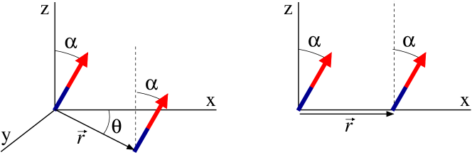
Figure 1: (Color online) Left: Two dipoles confined to move on the X-Y plane. The polarization field lays on the XZ plane and fixes a direction in space forming an angle $\alpha$ with the $z$ axis. $r$ and $\theta$ are polar coordinates in the X-Y plane. Right: Particular case of two dipoles on the X-Z plane ($y=0$).

We restrict our study to polarization angles where the interaction is fully repulsive, i. e. $\alpha\leq\alpha_{c}\approx 0.615$, where the stability of the system against collapse is ensured but the interaction may still show a high degree of anisotropy.

By means of diffusion Monte Carlo (DMC) simulations we evaluate the equation of state of the system, extending previous results Macia_2011 up to values of the density well above the mean-field regime, and show the effects of the anisotropy in the energy per particle and in some of the most relevant ground-state structural quantities of the system. We also present the excitation spectrum of the anisotropic gas in both the Bogoliubov and Feynman Feynman_1954 approximations. We compare these two approximations at low density, showing that they both agree well with each other. At higher densities, the Bogoliubov approximation breaks down, so we use the Feynman approximation to show how a roton minimum emerges and develops differently as a function of the direction in momentum space.

The rest of the paper is organized as follows. In Section II, we present DMC results for the ground state of the 2D gas of tilted dipoles. The effects of the anisotropic interaction in both the energy and structure properties when the density increases are discussed. In Section III, we calculate the excitation spectrum using the Feynman approximation, relying on the DMC results for the static structure functions, and compare it with the Bogoliubov spectrum. Also in this case, relevant signatures of the anisotropy are observed, mainly around the roton momenta. Finally, in Section IV we present the summary and conclusions of our work.

2 Ground state: energy and structure

We have studied the many-body properties of a two-dimensional gas of bosonic dipoles using the DMC method. DMC is a zero-temperature first-principles stochastic method which leads to exact properties of the ground state of bosonic systems. It is a form of Green’s Function Monte Carlo which samples the projection of the ground state from the initial configuration with the operator $\exp{\left[-(\mathcal{H}-E_{0})\tau\right]}$. Here, $\mathcal{H}$ is the Hamiltonian of the system, $E_{0}$ is a norm-preserving adjustable constant, and $\tau$ is the variable which corresponds to imaginary time. The simulation is performed by evolving in time $\tau$ by means of a combination of diffusion, drift and branching steps acting on walkers (sets of $2N$ coordinates) representing the wavefunction of the system.

The Hamiltonian of of $N$ fully polarized dipoles in two dimensions, written in dipolar units, is given by

$$H=-\frac{1}{2}\sum_{i=1}^{N}\nabla_{i}^{2}+\sum_{i<j}\frac{1-3\lambda^{2}\cos^{2}\theta_{ij}}{r_{ij}^{3}}\ ,$$ (3)

where $r_{ij}$ and $\theta_{ij}$ are the relative distance and polar angle formed by dipoles $i$ and $j$, respectively. This Hamiltonian is valid only when Van der Waals interaction can be neglected in front of dipolar forces. As we have commented in the previous Section, we restrict our study to polarization angles $\alpha<\alpha_{c}=0.615$, thus ensuring the potential is fully repulsive and the system is stable.

In order to guide properly the diffusion process and improve the variance of the results one introduces in the DMC method a trial wave function for importance sampling. In the present case, we use a variational Jastrow wave function of the form

$$\Psi(\textbf{r}_{1},...,\textbf{r}_{N})=\prod_{i<j}f(\textbf{r}_{ij})\ ,$$ (4)

where $\textbf{r}_{ij}=\textbf{r}_{i}-\textbf{r}_{j}$. Notice that due to the anisotropy of the system, the two-body correlation factor $f(\textbf{r})$ depends on the whole vector, rather than on its magnitude only. If the density is not high, the low-energy two-body scattering solution greatly influences the properties of the many body system, as three body scattering processes have extremely low probability. For this reason, we use as a Jastrow two-body correlation function the anisotropic zero-energy scattering solution Macia_2011 matched at some large distance, $\xi$, with the symmetrized form of a phononic wave function $f_{\text{ph}}(r_{ij})=exp(-C/r_{ij})$,Reatto_1967 $\xi$ being a variational parameter.

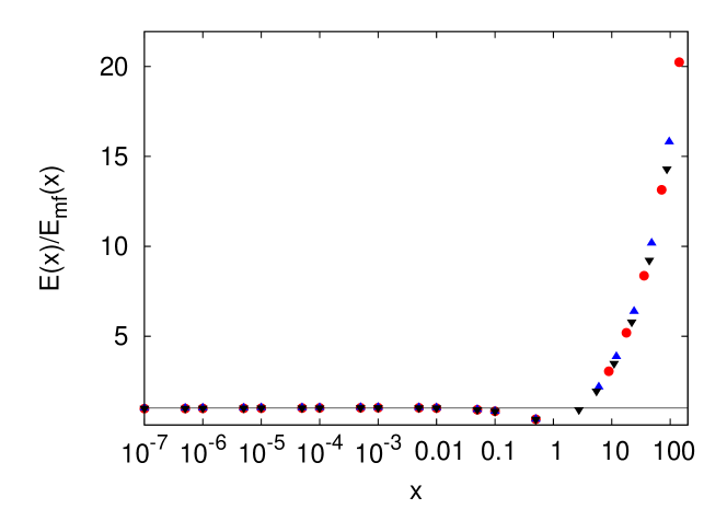
Figure 2: (Color online) Ratio of the energy per particle of the gas of dipoles for different polarization angles to the mean field prediction (5) as a function of the gas parameter $x=na^{2}$. Red circles, blue triangles and black inverted triangles correspond to $\alpha=0.2,0.4$ and $0.6$, respectively. The line corresponds to the mean field prediction.

Figure 2 shows the ratio of the energy per particle obtained from our DMC calculations and the mean field prediction Schick_1971

$$\frac{E_{MF}}{N}=\frac{\hbar^{2}}{2ma^{2}}\frac{4\pi x}{|\ln x|}\ ,$$ (5)

where $x=na^{2}$ is the gas parameter, with $n$ and $a$ being the density and the s-wave scattering length, respectively. We report results for three polarization angles $\alpha=0.2,0.4,0.6$. It is important to notice that, for a given value of the gas parameter $x$, different polarization angles imply different scattering length values and different densities. However, and as it can be seen from the figure, all energies corresponding to the same $x$ collapse into the same curve with very small deviations even at the higher densities considered. That means that the effects of the anisotropy of the interaction are accurately contained in the polarization dependent scattering length $a(\lambda)$, which is well approximated by the law Macia_2011

$$a(\lambda)=e^{2\gamma}\left(1-\frac{3\lambda^{2}}{2}\right)\ ,$$ (6)

where $\gamma=0.5772...$ is the Euler-Mascheroni constant and the factor $e^{2\gamma}$ corresponds to the s-wave scattering length of the isotropic dipolar system in 2D ($\alpha=0$) Ticknor_2009 . The scaling law observed in the energy, as reported in Fig. 2, may be also attributed to the small contributions to the energy coming from anisotropic terms (explicit $\theta$ terms) contained in the local energy estimator.

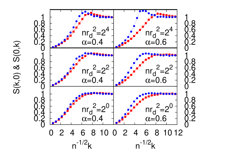
Figure 3: (Color online) Static structure function for polarization angles $\alpha=0.4$ and $\alpha=0.6$ for $nr_{d}^{2}=2^{4},2$ and $2^{0}$. Red squares and blue circles show the two cuts $S(k,0)$ and $S(0,k)$, respectively.

The anisotropic character of the dipole-dipole interaction has a direct influence on the ground-state wave function that is mirrored in the ground state expectation values of many-body operators. DMC allows us to evaluate pure estimations Casu_1995 of these observables. Contrarily to isotropic fluids, the static structure factor $S(\textbf{k})$, in the dipolar gas depends on the full vector $\textbf{k}=(k_{x},k_{y})$ rather than on its magnitude. Figure 3 shows two cuts of $S(\textbf{k})$ along the perpendicular and parallel directions with respect to the polarization plane, corresponding to the lines where the interaction is most and least repulsive, respectively. As expected, the effect of the anisotropy is more clearly seen at high densities and large polarization angles. In particular, for fixed $\alpha$ the separation between $S(k,0)$ and $S(0,k)$ is enhanced with increasing density. In much the same way the separation between the two cuts of the structure factor also increases for fixed density when the polarization angle is increased. At the largest densities considered, the effect of increasing the polarization angle makes the peak in $S(\textbf{k})$ increase in the strongly interacting direction and decrease in the weakly interacting one. This behavior is clearly observed in the Figure for the case $nr_{d}^{2}=2^{4}$ and $\alpha=0.6$.

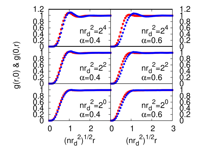
Figure 4: (Color online) Two-body distribution function for polarization angles $\alpha=0.4$ and $\alpha=0.6$ for $nr_{d}^{2}=2^{4},2$ and $2^{0}$. Red squares and blue circles show the two cuts $g(r,0)$ and $g(0,r)$, respectively.

The dependence of the interaction potential on the polar angle $\theta$ induces also changes in the distribution functions in different directions. We have calculated the two-body distribution function $g(\textbf{r})$ of the gas for different densities and polarization angles to visualize the effects of anisotropy in the spatial structure. As in the case of the static structure function, we have selected two cuts, $g(r,0)$ and $g(0,r)$, corresponding to the less and more repulsive directions. Selected results for the same densities and angles reported in Fig. 3 are shown in Fig. 4. As one can see, the anisotropy is also observed in the spatial structure but the effect is smaller than the one observed in $S(\textbf{k})$. Nevertheless, looking at the case ($nr_{d}^{2}=2^{4}$,$\alpha=0.6$) one observes that $g(r,0)$ has less structure than $g(0,r)$ which has a well defined first peak.

3 Excitation spectrum

A relevant issue in the study of tilted dipolar gases is the influence of the anisotropy of the interaction on the collective excitation spectrum. In this Section, we analyze this problem within two standard methods used currently in the study of Bose fluids: the Feynman and Bogoliubov approximations.

The Feynman spectrum is easy to derive from a simple sum rules argument and provides a single line in $(\textbf{k},\omega)$ space corresponding to a set of infinite lifetime excitations of energy Feynman_1954

$$\epsilon(\textbf{k})=\frac{\hbar^{2}k^{2}}{2mS(\textbf{k})}\ .$$ (7)

In this approximation, $\epsilon(\textbf{k})$ depends directly on the static structure factor, the only non-trivial quantity, and provides an upper bound to the actual excitation spectrum Boro_1995 . In systems like liquid ⁴He, this bound is closer to the experimental mode the lower the total momentum is.

On the other hand, we can study the excitation spectrum of the low density two-dimensional dipolar gas in the framework of the mean-field theory using the 2D time-dependent Gross-Pitaevskii equation,

$$i\hbar\frac{\partial\psi}{\partial t}=-\frac{\hbar^{2}}{2m}\nabla^{2}\psi+g|\psi|^{2}\psi\ ,$$ (8)

where $g$ is the 2D coupling constant $g=\frac{4\pi\hbar^{2}}{m}\frac{1}{|\log na^{2}|}$ Schick_1971 . Performing a standard Bogoliubov-deGennes linearization one finds the well-known Bogoiubov spectrum

$$\epsilon(\textbf{k})=\sqrt{\frac{\hbar^{2}k^{2}}{2m}\left(\frac{\hbar^{2}k^{2}}{2m}+2gn\right)}\ .$$ (9)

Although the spectrum obtained using this approach has contributions coming from the anisotropic character of the interaction due to the polarization angle dependence of the scattering length, not all contributions of the same order are taken into account. This simple Bogoliubov approach disregards the contribution coming from higher angular momentum channels, keeping only s-wave scattering processes. However, we know that different angular momentum channels couple in a non-trivial way in a dipolar system and so we have to take them into account. We know from the analysis of the zero-energy two-body problem that higher order partial wave contributions appear with higher orders in $\lambda^{2}$, so the leading corrections appear in $d$-wave. In order to consider the contribution of the d-wave we use the following pseudo-potential

$$V_{ps}(\textbf{r})=g\delta^{(2)}(\textbf{r})-\frac{C_{dd}}{4\pi}\frac{3\lambda^{2}\cos 2\theta}{r^{3}}$$ (10)

that leads to the following Gross-Pitaevskii equation

$$\begin{split}&i\hbar\frac{\partial\psi}{\partial t}=-\frac{\hbar^{2}}{2m}\nabla^{2}\psi+g|\psi|^{2}\psi-\\ \frac{C_{dd}}{4\pi}&\left(\int d\textbf{x}^{\prime}\frac{3\lambda^{2}\cos 2\theta}{|\textbf{x}-\textbf{x}^{\prime}|^{3}}|\psi(\textbf{x}^{\prime},t)|^{2}\right)\psi\ .\end{split}$$ (11)

The functional form of the pseudopotential $V_{ps}(\textbf{r})$ (10) as a sum of two terms, one isotropic and another anisotropic, follows the same prescription used in the three-dimensional problem Yi_2000 ; Derevianko_2003 . One can consider a linear perturbation of the condensate wave function of the system of the form

$$\psi(\textbf{x},t)=e^{-\frac{i}{\hbar}\mu t}(\sqrt{n}+\delta\psi(\textbf{x},t))\ ,$$ (12)

where the perturbative term $\delta\psi(\textbf{x},t)$ is given by

$$\delta\psi(\textbf{x},t)=ce^{i(\textbf{k}\cdot\textbf{x}-\omega t)}\ ,$$ (13)

where $c$ is the (small) perturbation amplitude.

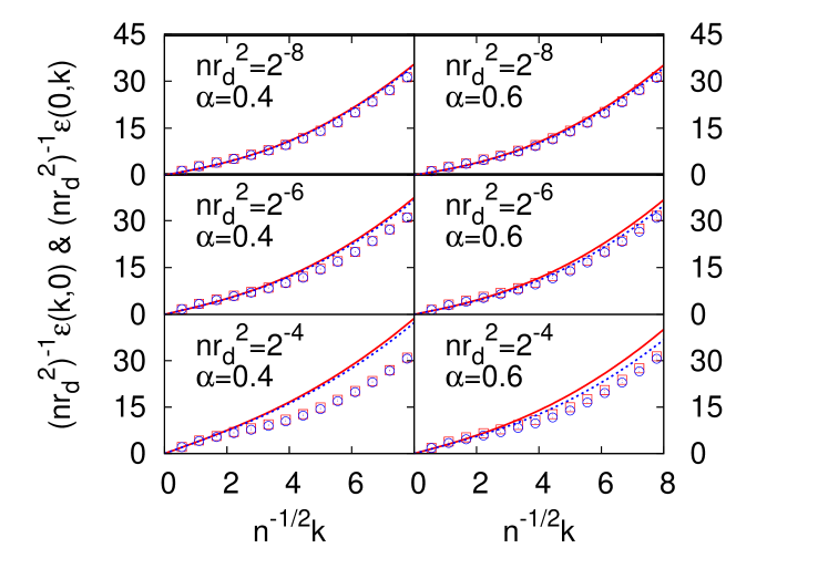
Figure 5: (Color online) Comparison of Feynman (symbols) and Bogoliubov (lines) excitation spectrum for angles $\alpha=0.4$ and $\alpha=0.6$ and $nr_{0}^{2}=2^{-4},2^{-6}$ and $2^{-8}$. Red solid and blue dashed curves show the two cuts $\epsilon(k,0)$ and $\epsilon(0,k)$ corresponding to Bogoliubov approximation respectively. Red open squares and Blue open circles show $\epsilon(k,0)$ and $\epsilon(0,k)$ corresponding to Feynman approximation respectively

By inserting (12) into Eq. (11), and neglecting non-linear terms, one finds the equation fulfilled by the small perturbation $\delta\psi$,

$$\begin{split}i\hbar\frac{\partial\delta\psi}{\partial t}=&-\frac{\hbar^{2}}{2m}\nabla^{2}\delta\psi+(2gn-\mu)\delta\psi+gn\delta\psi^{*}+\\ &n(F(\textbf{k})\delta\psi^{*}+F(-\textbf{k})\delta\psi)\ ,\end{split}$$ (14)

where $F(\textbf{k})$ is given by

$$F(\textbf{k})=\frac{C_{dd}}{4\pi}\left(\int d\textbf{y}\frac{3\lambda^{2}\cos 2\theta}{|\textbf{y}|^{3}}e^{i\textbf{k}\cdot\textbf{y}}\right),$$ (15)

and $\textbf{y}=\textbf{r}-\textbf{r}^{\prime}$. Now, taking into account that for a dilute homogeneous system the chemical potential is $\mu=gn$ and that for the two-dimensional dipole-dipole interaction $F(\textbf{k})=F(-\textbf{k})$, we finally arrive at the following expression for the Bogoliubov spectrum

$$\epsilon(\textbf{k})=\sqrt{\frac{\hbar^{2}k^{2}}{2m}\left(\frac{\hbar^{2}k^{2}}{2m}+2n(g+\pi k\lambda^{2}\cos 2\theta_{\textbf{k}})\right)}\ ,$$ (16)

where $\theta_{\textbf{k}}$ is the angle formed by the momentum of the excitation and the $x$-axis.

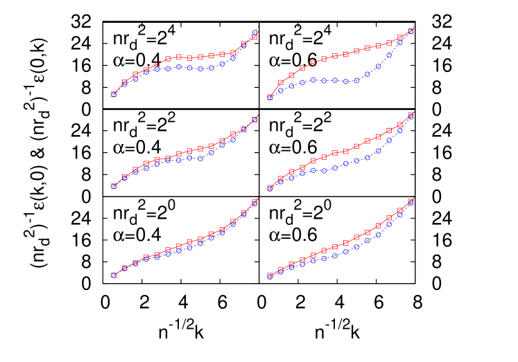
Figure 6: (Color online) Feynman excitation spectrum for angles $\alpha=0.4$ and $\alpha=0.6$ for $nr_{0}^{2}=2^{4},2$ and $2^{0}$. The red open squares and blue open circles show the two cuts $\epsilon(k,0)$ and $\epsilon(0,k)$, respectively.

The comparison between the Bogoliubov approximation given in this expression and the excitation spectrum obtained from DMC calculations using the Feynman approximation is shown in Fig. 5 for several values of the density and polarization angle. We can see from Fig. 5 that, as expected, the Bogoliubov and Feynman approximations coincide at very low densities. It is also noticeable the fact that, for a given value of the density, the Bogoliubov approximation is closer to the Feynman prediction at large polarization angles. This stresses once again that the relevant quantity describing the low density dipolar Bose gas is the gas parameter $x=na^{2}$, and according to equation (6) the scattering length $a(\lambda)$ decreases with increasing polarization angle. For a fixed density, $x$ decreases when $\alpha$ increases, and the Feynman prediction gets closer to the Bogoliubov mode, which is know to successfully characterize the excitation spectrum of Bose gases when $x\rightarrow 0$. We can conclude from Fig. 5 that Feynman and Bogoliubov approximations are close to each other at small values of the momentum $k$. Finally, one also sees that the excitation spectrum becomes isotropic when $k\rightarrow 0$.

Furthermore, the Bogoliubov approximation is expected to be valid only at very low densities while the Feynman approximation is known to provide an upper bound to the exact excitation spectrum of the system. To have some insight on how $\epsilon(\textbf{k})$ evolves with the density we show in Figure 6 the Feynman mode at higher values of $n$. The results presented in the figure correspond to densities that are still far from the crystallization point of the isotropic system  Buchler_2007 ; Astra_2007 . From Fig. 6, one can see that with increasing density the spectrum develops a roton-like minimum which for fixed density and polarization angle is deeper in the most repulsive direction. It is interesting to notice that as the anisotropy of the interaction is increased,i.e., when the polarization angle grows, the roton minimum is deeper in the more repulsive direction while in the orthogonal direction the spectrum does not show any minimum in the range of considered densities. In fact, the emergence of the roton and its eventual zero-energy limit has been discussed as a clear signature of the instability of the system when the critical polarization angle is higher than $\alpha_{c}$ Santos_2003 ; Hufnagl_2011 .

4 Summary and Conclusions

To summarize, in this work we have described some properties of a two-dimensional dipolar Bose gas where the polarization field forms an angle $\alpha$ with the normal direction. The projection of the polarization vector on the plane defines the x-axis, where the interaction potential is weaker than in any other direction. In this situation there is a critical polarization angle $\alpha_{c}=0.615$ where the potential starts to show attractive regions. We have used the two-body zero energy wave function to build a many-body Bijl-Jastrow wave function that we used as an input for our diffusion Monte Carlo simulations of the homogeneous polarized dipolar Bose gas. We have presented results for the energy per particle in comparison with the well known mean field prediction of the two dimensional equation of state at low densities. The scaling of the energy in the gas parameter is preserved up to values of $x$ much larger than those of the mean-field regime, corresponding to values $x\leq 10^{-2}$, in which the energy only depends on the gas parameter and not on the specific interaction.

In the second part, we have studied the excitation spectrum of the system in two different frameworks, the Bogoliubov and Feynman approximations. We have shown that the agreement between these two approaches is very good at very low densities as it was expected. We have derived the first anisotropic correction to the Bogoliubov spectrum, and we have shown that in the range of validity of the Bogoliubov approximation the anisotropy plays an extremely small role. At higher densities, the Feynman approximation predicts a strongly anisotropic spectrum showing a roton-like minimum that depends on the direction of the momentum.

- (1) A. Griesmaier, J. Werner, S.Hensler, J.Stuhler, and T. Pfau, Phys. Rev. Lett. 94, 160401 (2005).
- (2) J. Stuhler, A. Griesmaier, T. Koch, M. Fattori, T. Pfau, S. Giovanazzi, P. Pedri, and L. Santos, Phys. Rev. Lett. 95, 150406 (2005).
- (3) K.-K. Ni, S. Ospelkaus, M. H. G. de Miranda, A. Pe’er, B. Neyenhuis, J. J. Zirbel, S. Kotochigova, P. S. Julienne, D. S. Jin, and J. Ye, Science 322, 231 (2008).
- (4) S. Ospelkaus, A. Pe’er, K. K. Ni, J. J. Zirbel, B. Neyenhuis, S. Kotochigova, P. S. Julienne, J. Ye, and D. S. Jin, Nature Phys. 4, 622 (2009).
- (5) K.-K. Ni, S. Ospelkaus, D. Wang, G. Quéméner, B. Neyenhuis, M. H. G. de Miranda, J. L. Bohn, J. Ye, and D. S. Jin, Nature 464, 1324 (2010).
- (6) M. Lu, N. Q. Burdick, S. H. Youn and B. L. Lev, Phys. Rev. Lett. 107, 19041 (2011).
- (7) M. Lu, N. Q. Burdick and B. L. Lev, Phys. Rev. Lett. 108 215301 (2012).
- (8) K. Aikawa, A. Frisch, M. Mark, S. Baier, A. Rietzler, R. Grimm and F. Ferlaino, Phys. Rev. Lett. 108 210401 (2012).
- (9) L. Santos, G. V. Shlyapnikov, P. Zoller and M. Lewenstein, Phys. Rev. Lett. 85 1791 (2000).
- (10) L. Santos, G. V. Shlyapnikov and M. Lewenstein, Phys. Rev. Lett. 90 250403 (2003).
- (11) C. Ticknor, Phys. Rev. A 80, 052702 (2009).
- (12) C. Ticknor, Phys. Rev. A 81, 042708 (2010).
- (13) C. Ticknor, Phys. Rev. A 84, 032702 (2011).
- (14) Y. Cai, M. Rosenkranz, Z. Lei and W. Bao, Phys. Rev. A 82, 043623 (2010).
- (15) H. P. Buchler, E. Demler, M. Lukin, A. Micheli, N. Prokof’ev, G. Pupillo and P. Zoller, Phys. Rev. Lett. 98, 060404 (2007).
- (16) G. E. Astrakharchik, J. Boronat, I. L. Kurbakov and Y. E. Lozovik, Phys. Rev. Lett. 98, 060405 (2007).
- (17) G. E. Astrakharchik, J. Boronat, J. Casulleras, I. L. Kurbakov and Y. E. Lozovik, Phys. Rev. A 79, 051602 (2009).
- (18) A. Filinov, N. V. Prokof’ev and M. Bonitz, Phys. Rev. Lett. 105, 070401 (2010).
- (19) A. Macia, F. Mazzanti, J. Boronat, and R. E. Zillich, Phys. Rev. A 84, 033625 (2011).
- (20) F. Mazzanti, R. E. Zillich, G. E. Astrakharchik, and J. Boronat, Phys. Rev. Lett. 102, 110405 (2009).
- (21) C. Ticknor, R. M. Wilson, and J. L. Bohn, Phys. Rev. Lett. 106, 065301 (2011).
- (22) D. Hufnagl, R. Kaltseis, V. Apaja and R. E. Zillich, Phys. Rev. Lett. 107, 065303 (2011).
- (23) R. P. Feynman, Phys. Rev. 94, 262 (1954).
- (24) L. Reatto and G. V. Chester, Phys. Rev. 155, 88 (1967).
- (25) M. Schick, Phys. Rev. A 3, 1067 (1971).
- (26) J. Casulleras and J. Boronat, Phys. Rev. B 52, 3654 (1995).
- (27) J. Boronat, J. Casulleras, F. Dalfovo, S. Stringari and S. Moroni, Phys. Rev. B 52, 1236 (1995).
- (28) S. Yi and L. You, Phys. rev. A 63, 053607 (2000).
- (29) A. Derevianko, Phys. Rev. A 67, 033607 (2003).