Chemical evolution of the Large Magellanic Cloud

Abstract

We adopt a new chemical evolution model for the Large Magellanic Cloud (LMC) and thereby investigate its past star formation and chemical enrichment histories. The delay time distribution of type Ia supernovae recently revealed by type Ia supernova surveys is incorporated self-consistently into the new model. The principle results are summarized as follows. The present gas mass fraction and stellar metallicity as well as the higher [Ba/Fe] in metal-poor stars at [Fe/H]$<-1.5$ can be more self-consistently explained by models with steeper initial mass functions. The observed higher [Mg/Fe] ($\geq 0.3$) at [Fe/H]$\sim-0.6$ and higher [Ba/Fe] ($>0.5$) at [Fe/H]$\sim-0.3$ can be due to significantly enhanced star formation about 2 Gyr ago. The observed overall [Ca/Fe]–[Fe/H] relation and remarkably low [Ca/Fe] ($<-0.2$) at [Fe/H]$>-0.6$ are consistent with models with short-delay supernova Ia and with the more efficient loss of Ca possibly caused by an explosion mechanism of type II supernovae. Although the metallicity distribution functions do not show double peaks in the models with a starburst about 2 Gyr ago, they show characteristic double peaks in the models with double starbursts at $\sim 200$ Myr and $\sim 2$ Gyr ago. The observed apparent dip of [Fe/H] around $\sim 1.5$ Gyr ago in the age–metallicity relation can be reproduced by models in which a large amount ($\sim 10^{9}M_{\odot}$) of metal-poor ([Fe/H]$<-1$) gas can be accreted onto the LMC.

1 Introduction

The time evolution of the chemical abundances in the interstellar medium (ISM), field stars, and globular clusters (GCs) of the Large Magellanic Cloud (LMC) contains valuable information on its long-term star formation history and thus has been investigated in detail by many authors (e.g., Da Costa 1991; Olszewski et al. 1991; Russel & Dopita 1992; Dopita et al. 1997; Geisler et al. 1997; Pagel & Tautvaišiené 1998, PT98; Cole et al. 2005, C05; Cioni et al. 2006). The elemental abundance ratios of $\alpha$ ($\alpha$ means alpha-elements), Fe-peak, and neutron-capture elements in field stars and GCs of the LMC have been extensively investigated by spectroscopic observations. The observed differences in the abundance ratios between the LMC and the Galaxy have been discussed in detail (e.g., Hill et al. 1995, 2000; Johnson et al. 2006). The radial and azimuthal variations of stellar metallicities in the the LMC disk has been investigated both observationally and theoretically in terms of its star formation and dynamical evolution histories (Geisler et al. 2003; Bekki & Chiba 2005; Cioni et al. 2006).

One of the importance results in these previous studies is that the observed age–metallicity relation (AMR) is more consistent with a model with a secondary “starburst” about a few Gyr ago in the LMC (e.g., Tsujimoto et al. 1995, T95; PT98). Although the possible presence of a past starburst (or significantly enhanced star formation) has long been discussed in other observational studies (e.g., Butcher 1977; Stryker 1983; Bica et al. 1986; Bertelli et al. 1992; Olszewski et al. 1996; Gallagher et al. 1996; Vallenari et al. 1996; Ardeberg et al. 1997; Elson et al. 1997; Geha et al. 1998 Holzman et al. 1998, 1999; Olsen 1999; Smecker-Hane et al. 2002; Glatt et al. 2010; Indu & Subramaniam 2011), the epoch and the strength of the burst were not well constrained. Furthermore, owing to the lack of modern chemical evolution models with the latest chemical yields of asymptotic giant branch (AGB) stars and supernovae, it remained unclear how the long-term star formation history with a possible starburst could be imprinted on the detailed elemental abundance ratios of field stars and GCs in the LMC.

Recent photometric and spectroscopic observations of field stars and GCs have provided new clues for these unresolved problems in the LMC. For example, photometric studies of the stellar populations in the LMC have revealed the AMRs of different local regions in the LMC disk (e.g., Harris & Zaritsky 2009, HZ09; Rubele et al. 2012, R12). The AMR derived by HZ09 show enhanced star formation rates of the LMC around 2 Gyr, 500 Myr, 100 Myr, and 12 Myr with the two peaks (500 Myr and 2 Gyr) being nearly coincident with the star formation peaks observed in the SMC. Piatti (2011) has also shown that there was a burst of cluster formation around 2 Gyr in the LMC and suggested that the LMC experienced strong tidal interaction with the SMC and possibly with the Galaxy. Using deep near-infrared data from the VISTA near-infrared YJK_s survey of the Magellanic system, R12 derived the star formation histories of different local regions in the LMC disk. They revealed the presence of peaks in SFRs around 3 Gyr and 5 Gyr ago for most of the subregions. Glatt et al. (2010) have recently found an enhanced cluster formation at 125 Myr and 800 Myr ago in their 324 populous star clusters for the LMC.

Furthermore, recent spectroscopic observations of field stars and GCs in the LMC have revealed intriguing chemical properties of the LMC (e.g., Mucciarelli et al. 2008, Pompéia et al. 2008, P08; Colucci et al. 2012, C12, Haschke et al. 2012). Mucciarelli et al. (2008) have shown that all four of the intermediate-age GCs which they investigated in the LMC have negligible star-to-star scatter in their chemical abundances of light, $\alpha$, iron-peak and neutron-capture elements. This implies that secondary star formation from gaseous ejecta of stars within the GCs did not occur so that the chemical abundances might be similar between intermediate-age field stars and clusters. P08 have found that [Ca/Fe] and [Si/Fe] in the LMC stars are lower than those of the Galactic stars at the same [Fe/H] whereas the [O/Fe] and [Mg/Fe] are only slightly deficient in comparison with their Galactic counterparts. C12 have revealed the age-dependence of [$\alpha$/Fe] and [Fe/H] among globular/star clusters with ages between 0.05 and 12 Gyr and the significant enhancement of the neutron-capture elements Ba, La, Nd, Sm, and Eu in the youngest star clusters. The origin of these recent observational results has not yet been treated by chemical evolution models.

In spite of this progress in observational studies of the stellar populations of the LMC, theoretical models to explain the observations have not yet been fully developed. T95 tried to explain the observed [O/Fe]–[Fe/H] relation, the metallicity distribution function (MDF), and the AMR in a self-consistent manner by adopting a model in which the LMC had a starburst about 3 Gyr ago and a steeper initial mass function (IMF). They explained these observations, though the observational data points are much smaller than those that we can now access. Pilyugin (1996) demonstrated that the observed [Fe/O] versus [Fe/H] relation can be reproduced only by the galactic wind model in which stellar ejecta can be preferentially expelled from the LMC. PT98 explained the observed AMR and chemical abundance patterns of the LMC by considering “non-selective stellar wind” models in which some fraction of the stellar ejecta both from AGB stars and SNe can be expelled completely from the LMC and consequently can not participate in the chemical enrichment processes. These previous chemical evolution models did not incorporate the delay time distribution (DTD) of type Ia supernova (SNe Ia) recently revealed by extensive SN Ia surveys (e.g., Mannucci et al. 2006; Sullivan et al. 2006; Totani et al. 2008; Maoz et al. 2010) and thus might not be regarded as realistic and reasonable. The construction of more sophisticated and realistic models is indispensable for discussing the above mentioned latest observational results.

The purpose of this paper is to adopt a new chemical evolution model and thereby discuss the latest observational results on the chemical evolution and star formation history of the LMC. The observed DTD of SNe Ia is adopted in the new model so that the progenitor stars of SNe Ia can explode as early as $10^{8}$yr after their formation. These “prompt SNe Ia” can cause fundamental differences in the chemical evolution between the present model and previous ones (e.g., T95) in which the time delay between star formation and explosion of SNe Ia is assumed to be typically $\sim 10^{9}$ yr (“classical SNe Ia”). The new model also incorporates the metallicity dependent chemical yields of AGB stars (e.g., Busso et al. 2001; Tsujimoto & Bekki 2012; TB12) so that the chemical evolution of $s$-process elements can be investigated and compared with the observations. The new model is the so-called “one-zone” model, in which the time evolution of averaged chemical properties can be investigated.

We explore a wide range of models with and without starburst and different star formation histories in the LMC so that we can discuss recent new observational results on different chemical properties of the LMC disk stars. For example, we will discuss (i) whether and how the previous starburst(s) triggered by the LMC–SMC–Galaxy interaction can be imprinted on the chemical abundance properties of the LMC, (ii) how the IMF can control the chemical evolution, and (iii) how the accretion of metal-poor gas from the SMC or high velocity clouds onto the LMC (Bekki & Chiba 2007, BC07; Diaz & Bekki 2012, DB12; Bekki & Tsujimoto 2010) influences the chemical evolution. It is timely to discuss the chemical evolution of the LMC in the context of the Galaxy–LMC–SMC tidal interaction, given that recent observational and theoretical studies have demonstrated that the tidal interaction is important not only for the star formation history of the LMC but also for the stellar and gaseous distributions of the Magellanic system (e.g., Olsen et al. 2011; DB12).

The layout of this paper is as follows. In §2, we describe our new one-zone chemical evolution models in detail. In §3, we present the results of the time evolution of the chemical abundances for models with different parameters. In §4, we discuss the results in the context of the IMF, the long-term star formation history, and the gas accretion events in the LMC. The conclusions of the present study are given in §5.

2 The model

2.1 Basic equations

We adopt one-zone chemical evolution models that are essentially the same as those adopted in our previous studies on the chemical evolution of the Galaxy (Tsujimoto et al. 2009; TB12). Accordingly, we briefly describe the adopted models in the present study. The present model is improved in comparison with previous ones (Tsujimoto et al. 2009) in terms of including the $s$-process elements and prompt SNIa self-consistently in the models. The LMC disk is assumed to form through a continuous gas infall from outside the disk region (e.g., halo) for the last 13 Gyr, as in previous chemical evolution models (e.g., Tsujimoto et al. 2009). Some fraction of gas with metals can be expelled from the LMC as stellar winds through energetic feedback effects of SNe in some models of the present study (e.g., “wind models”, as described later). The star formation can be suddenly and significantly enhanced (referred to as “bursts of star formation” or “starburst”). As demonstrated by theoretical studies, the Galaxy–LMC–SMC tidal interaction is important both for the formation of the Magellanic Stream and for reproducing the observed peaks of star formation in the LMC (e.g., Bekki & Chiba 2005; DB12). Therefore, the adopted assumption of starburst is quite reasonable. Although the infall of metal-poor gas from the SMC and other dwarf galaxies can be important for the LMC chemical evolution, we discuss this later in §4.

We investigate the time evolution of the gas mass fraction ($f_{\rm g}(t)$), the star formation rate ($\psi(t)$), and the abundance of the $i$th heavy element ($Z_{i}(t)$) for a given accretion rate ($A(t)$), IMF, and ejection rate of ISM ($w(t)$). The basic equations for the adopted one-zone chemical evolution models are described as follows:

$$\frac{df_{g}}{dt}=-\alpha_{\rm l}\psi(t)+A(t)-w(t)$$ (1)

$$\frac{d(Z_{i}f_{g})}{dt}=-\alpha_{\rm l}Z_{i}(t)\psi(t)+Z_{A,i}(t)A(t)+y_{{\rm II},i}\psi(t)$$

$$+y_{{\rm Ia},i}\int^{t}_{0}\psi(t-t_{\rm Ia})g(t_{\rm Ia})dt_{\rm Ia}$$

$$+\int^{t}_{0}y_{{\rm agb},i}(m_{\rm agb})\psi(t-t_{\rm agb})h(t_{\rm agb})dt_{\rm agb}-W_{i}(t)\ \ ,$$ (2)

where $\alpha_{\rm l}$ is the mass fraction locked up in dead stellar remnants and long-lived stars, $y_{\rm{Ia},i}$, $y_{\rm{II},i}$, and $y_{\rm{agb},i}$ are the chemical yields for the $i$th element from type II supernovae (SN II), from SN Ia, and from AGB stars, respectively, $Z_{A,i}$ is the abundance of heavy elements contained in the infalling gas, and $W_{i}$ is the wind rate for each element. The quantities $t_{\rm Ia}$ and $t_{\rm agb}$ represent the time delay between star formation and SN Ia explosion and that between star formation and the onset of AGB phase, respectively. The terms $g(t_{\rm Ia}$) and $h_{\rm agb}$ are the distribution functions of SNe Ia and AGB stars, respectively, and the details of which are described later in this section. The term $h_{\rm agb}$ controls how much AGB ejecta can be returned into the ISM per unit mass for a given time in equation (2). The total gas masses ejected from AGB stars depends on the original masses of the AGB stars (e.g., Weidemann 2000). Therefore, this term $h_{\rm agb}$ depends on the adopted IMF and the age–mass relation of the stars (later described). Thus equation (1) describes the time evolution of the gas due to star formation, gas accretion, and stellar wind. Equation 2 describes the time evolution of the chemical abundances due to chemical enrichment by supernovae and AGB stars.

The star formation rate $\psi(t)$ is assumed to be proportional to the gas fraction with a constant star formation coefficient and thus is described as follows:

$$\psi(t)=C_{\rm sf}f_{\rm g}(t)$$ (3)

We assume that $C_{\rm sf}$ is different between (i) the “quiescent phase”, when the LMC shows an almost steady star formation, and (ii) the “burst phase”, when the LMC experienced a burst of star formation. In the present study, we investigate models with no burst (referred to as “standard models”) and those in which a starburst can occur only once (“burst models”) and twice (“double-burst models”). The star formation rate is assumed to be constantly higher for $t_{\rm sb1,s}\leq t\leq t_{\rm sb1,e}$ in the first starburst and $t_{\rm sb2,s}\leq t\leq t_{\rm sb2,e}$ in the second one. The star formation coefficient ($C_{\rm sf}$) is thus described as follows:

$$C_{\rm sf}=\left\{\begin{array}[]{ll}C_{q}&\mbox{for quiescent phase}\\ C_{\rm sb1}&\mbox{for first starburst}\\ C_{\rm sb2}&\mbox{for second starburst}\\ \end{array}\right.$$ (4)

In the present study, a non-dimensional value of $C_{\rm sf}$ is given for each model.

For the accretion rate, we adopt the formula in which $A(t)=C_{\rm a}\exp(-t/t_{\rm a})$ and $t_{\rm a}$ is a free parameter controlling the time scale of the gas accretion. The normalization factor $C_{\rm a}$ is determined such that the total gas mass accreted onto the LMC can be 1 for a given $t_{\rm a}$. Although we investigated models with different $t_{\rm a}$, we finally adopt the models with $t_{\rm a}=0.3$ Gyr as reasonable ones for the LMC. This is mainly because the models with $t_{\rm a}=0.3$ Gyr can better explain the observations. The present results do not depend strongly on the parameter $t_{\rm a}$ for a reasonable parameter range. The initial [Fe/H] of the infalling gas is set to be $-2$ and we assume a SN-II like enhanced [$\alpha$/Fe] ratio (e.g., [Mg/Fe]$\approx 0.4$) and [Ba/Fe] for the gas. This adoption of initial [Fe/H] is reasonable for the present study which discusses stars with [Fe/H] as low as $-2$. Also, such adoption has been done in other chemical evolution models (e.g., Tsujimoto et al. 2009). We discuss our parameter study for the above variables in §2.5.

2.2 Selective and non-selective stellar winds

We investigate models in which metals from AGB stars and SNe can be removed from the LMC through energetic stellar winds so that they can not be used for chemical enrichment of the LMC ISM. These models are referred to as “wind models” for convenience. The wind models are further divided into two categories: “selective wind models” and “non-selective wind models”. Only SNe ejecta (not already existing ISM) can be expelled from the LMC in the selective wind model, whereas both ejecta from SNe and AGB stars and already existing ISM can be expelled from the LMC in the non-selective wind model. For comparison, we also investigate models in which there is no stellar wind and thus gaseous ejecta from all stars can be fully mixed with the ISM (“non-wind models”).

In the selective wind models, some fraction, $1-f_{\rm ej}$, of gaseous ejecta from SNe can be mixed with ISM for chemical enrichment processes whereas all AGB ejecta can be mixed with ISM. Therefore, the wind rate $w(t)$ is estimated only from the total mass of gaseous ejecta from SNe $M_{\rm ej,sn}$ at each time step. The total mass, $M_{\rm w}$, of ISM that is removed from the LMC at each time step in the selective wind models is

$$M_{\rm w}=f_{\rm ej}M_{\rm ej,sn}.$$ (5)

In the non-selective wind models, we adopt the same model as that used in PT98 in which $M_{\rm ej}$ is determined solely by the star formation rate:

$$M_{\rm w}=C_{\rm ej}\psi(t),$$ (6)

where $C_{\rm ej}$ is a parameter (in simulation units) that can control how efficiently the ISM with AGB and SN ejecta can be removed from the LMC. We investigate non-wind (i.e., standard, burst, non-burst), selective wind, and non-selective wind models. We discuss our parameter study for the above variables in §2.5.

2.3 Chemical yields and delay time distribution of SN Ia

We adopt the nucleosynthesis yields of SNe II and Ia from T95 to deduce $y_{{\rm II},i}$ and $y_{{\rm Ia},i}$ for a given IMF. Stars with masses larger than $8M_{\odot}$ explode as SNe II soon after their formation and eject their metals into the ISM. In contrast, there is a time delay ($t_{\rm Ia}$) between the star formation and the metal ejection for SNe Ia. We here adopt the following DTD ($g(t_{\rm Ia}$)) for 0.1 Gyr $\leq t_{\rm Ia}\leq$ 10 Gyr, which is consistent with recent observational studies on the SN Ia rate in extra-galaxies (e.g., Totani et al. 2008; Maoz et al. 2010, 2011):

$$g_{\rm Ia}(t_{\rm Ia})=C_{\rm g}t_{\rm Ia}^{-1},$$ (7)

where $C_{\rm g}$ is a normalization constant that is determined by the number of SN Ia per unit mass (which is controlled by the IMF and the binary fraction for intermediate-mass stars for the adopted power-law slope of $-1$). Maoz & Badens (2010) detected a population of prompt SNIa in the LMC and showed that the number of prompt SNIa per stellar mass formed is $2.7-11.0\times 10^{-3}M_{\odot}^{-1}$. Although we mainly investigate the “prompt SN Ia models” with the above DTD, we also investigate the “classical SN Ia models” with 1 Gyr $\leq t_{\rm Ia}\leq$ 3 Gyr (e.g., Yoshii et al. 1996). This SNIa lifetime in Yoshii et al. (1996) was deduced by using their Galactic chemical evolution models that can be consistent with the observed [O/Fe]–[Fe/H] relations of the Galactic stars in the solar neighborhood. The fraction of the stars that eventually produce SNe Ia for 3–8$M_{\odot}$ has not been observationally determined and thus is regarded as a free parameter, $f_{\rm b}$. We mainly investigate models with $f_{\rm b}=0.03$, because such models can better explain the observed chemical properties of the LMC. We briefly compare the results of models with $f_{\rm b}=0.03$ and $0.06$. For the site of r-process, we adopt the mass range of 8–10$M_{\odot}$ for SNe II (Mathews et al. 1992; Ishimaru et al. 1999) as identified with the collapsing O-Ne-Mg core (Wheeler et al. 1998). The yield of Ba from r-process is $1.45\times 10^{-6}M_{\odot}$ for the adopted range of SNe II.

Low-mass AGB stars ($<3M_{\odot}$) release the $s$-process elements during the thermally pulsing AGB phase (e.g., Gallino et al. 1998). As a consequence of large uncertainties in convective mixing and ¹³C-pocket efficiencies, the $s$-process nucleosynthesis allows for a wide range of possible production levels. On the other hand, the observed abundances for the AGB stars can be directly compared with the theoretical nucleosynthesis results. Here we investigate the element Ba by adopting the best empirical metallicity dependent Ba-yield derived by TB12. The adopted metallicity dependent Ba-yield $y_{\rm Ba}$ is

$$y_{\rm Ba}=\left\{\begin{array}[]{ll}y_{\rm Ba,0}(m_{\rm agb})\times 10^{1.5{\rm[Fe/H]}+1.5}&-2\leq{\rm[Fe/H]}<-1\\ y_{\rm Ba,0}(m_{\rm agb})&-1\leq{\rm[Fe/H]}\\ \end{array}\right.$$ (8)

The value of $y_{\rm Ba,0}(m_{\rm agb})$ depends on the mass of the stars $m_{\rm agb}$ that can finally become AGB stars. The adopted $y_{\rm Ba,0}(m_{\rm agb})$ are $2.6\times 10^{-7}M_{\odot}$, $4.0\times 10^{-7}M_{\odot}$, and $5.2\times 10^{-7}M_{\odot}$ for $m_{\rm agb}=1.5M_{\odot}$, $2.0M_{\odot}$, and $3.0M_{\odot}$, respectively.

An AGB star with initial mass $m_{\rm I}$ and final mass $m_{\rm F}$ can eject its envelope with a total mass of $m_{\rm ej}$ and the gas can be mixed with the surrounding ISM to chemically pollute the ISM. The initial-to-final relationship for AGB stars, from which we can deduce $m_{\rm ej}$, has been extensively discussed in Weidemann (2000). We derive an analytic form for $m_{\rm ej}$ ($=m_{\rm I}-m_{\rm F}$) from the observational data by Weidemann (2000) by using the least squares fitting method, and find

$$m_{\rm ej}=0.916M_{\rm I}-0.444.$$ (9)

The coefficient of determination ($R$-value) is 0.995 for the above fitting. In order to calculate the main-sequence turn-off mass $m_{\rm TO}$, we use the following formula (Renzini & Buzzoni 1986):

$$\log m_{\rm TO}(t_{\rm s})=0.0558(\log t_{\rm s})^{2}-1.338\log t_{\rm s}+7.764,$$ (10)

where $m_{\rm TO}$ is in solar units and time $t_{\rm s}$ is in years. By using the adopted IMF and equations (9) and (10), we numerically estimate $h_{\rm agb}$ (i.e., how much AGB ejecta can be returned into ISM per unit mass) in equation (2) at each time step.

2.4 IMF

The adopted IMF is defined as $\Psi(m_{\rm I})=M_{s,0}{m_{\rm I}}^{-\alpha}$, where $m_{\rm I}$ is the initial mass of each individual star and the slope $\alpha=2.35$ corresponds to the Salpeter IMF (Salpeter 1955). The normalization factor $M_{s,0}$ is a function of $\alpha$, $m_{\rm l}$ (lower mass cut-off), and $m_{\rm u}$ (upper mass cut-off). These $m_{\rm l}$ and $m_{\rm u}$ are set to be $0.1{\rm M}_{\odot}$ and $50{\rm M}_{\odot}$, respectively (so that the normalization factor $M_{s,0}$ is dependent simply on $\alpha$). We investigate models with different $\alpha$ to find the model(s) that can best explain the observed abundance patterns of stars in the LMC. We do not discuss models with different $m_{\rm u}$, because the effects of changing $m_{\rm u}$ on the LMC chemical evolution are similar to those of changing $\alpha$.

2.5 Parameter studies

We mainly investigate the standard (labeled as “S”), burst (“B”), and double-burst (“DB”) models in which stellar wind effects are not included at all (i.e., “non-wind models”). By using these non-wind models, we demonstrate how the IMF slope ($\alpha$) and the epochs of starburst ($t_{\rm sb1,s}$ and $t_{\rm sb2,s}$) can influence the chemical evolution of the LMC. These $t_{\rm sb1,s}$ and $t_{\rm sb2,s}$ are given in units of Gyr. We then investigate the wind models (“W”) so that we can discuss whether or not removal of AGB and SN ejecta from the LMC is important in the chemical evolution of the LMC. In the present study, the time $t$ is the time that has elapsed since the model calculation started. Therefore $t=0$ Gyr (13 Gyr) represent the time when the calculation starts (ends). Previous observational and theoretical studies have suggested that there could be at least two epochs of enhanced star formation (starburst) about $\sim 2$ Gyr ago and $0.2$ Gyr ago (e.g., HZ09 and DB12). We therefore mainly investigate the burst and double-burst models with $t_{\rm sb1,s}=11$ Gyr and $t_{\rm sb2,s}=12.8$ Gyr. Table 1 summarizes the representative 26 models investigated in the present study.

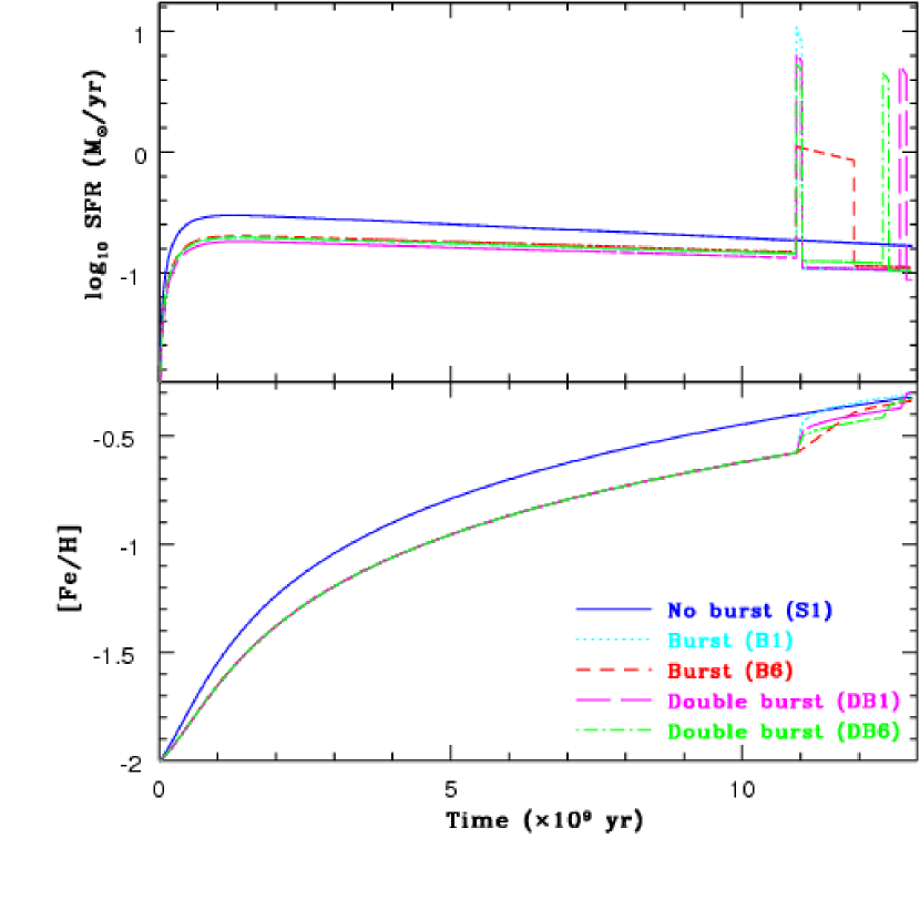
Figure 1: The time evolution of star formation rates (SFRs) in units of $M_{\odot}$ yr^-1 (upper) and [Fe/H] (lower) for the five representative models with different star formation histories, S1 (blue solid), B1 (cyan dotted), B6 (red short-dashed), DB1 (magenta long-dashed), and DB 6 (green dot-dashed). The SFRs are estimated for these models by assuming that the present total stellar mass of the LMC ($M_{\rm s}$) is $2.7\times 10^{9}M_{\odot}$.

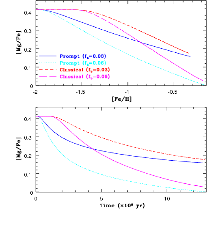
Figure 2: Chemical evolution of four models on the [Mg/Fe]-[Fe/H] plane (upper) and the time evolution of [Mg/Fe] for two prompt SN Ia models with $f_{\rm b}=0.03$ (blue solid) and 0.06 (cyan dotted) and two classical SN Ia ones with $f_{\rm b}=0.03$ (red short-dashed) and 0.06 (magenta long-dashed).

Figure 1 illustrates the time evolution of star formation rates (SFRs) and [Fe/H] of stars in the five representative models (S1, B1, B6, DB1, and DB6) with different parameters controlling the LMC star formation history. No burst of star formation is assumed in S1 whereas only one burst is assumed in B1 and B6. Two bursts of star formation at different epochs are assumed in DB1 and DB6. These models are chosen so that they can, in combination, show a wide range of star formation histories in Figure 1: they are just examples of possible star formation histories of the LMC. We investigate how the final chemical abundances depend on the LMC star formation history by using the results of models with different star formation histories. Figure 2 shows the time evolution of [Mg/Fe] and the [Mg/Fe]–[Fe/H] relation in the models with prompt and classical SNe Ia. It is clear from this figure that the models with prompt SN Ia show no plateau in the [Mg/Fe]–[Fe/H] relation owing to the earlier chemical enrichment by SNe Ia that can eject an Fe-rich gas. Figure 2 also shows that the time evolution of [Mg/Fe] depends on $f_{\rm b}$ in such a way that [Mg/Fe] can steeply decrease with time in the model with larger $f_{\rm b}$. We discuss these in more detail for different models in the following sections.

2.6 Observations to be compared with predictions

We mainly investigate (i) the present gas mass fraction $f_{\rm g,0}$, (ii) the stellar metallicity of the youngest stellar population, [Fe/H]₀, (iii) AMR, (iv) [Mg/Fe]–[Fe/H] relation (as an example of [$\alpha$/Fe]–[Fe/H] relations), (v) [Ba/Fe]–[Fe/H] relation (as an example of the time evolution of $s-$process elements), and (vi) MDF. We compare these results with the corresponding observations for the LMC. In order to demonstrate clearly how different chemical properties of the LMC are compared with those of the Galaxy, we also show the observational results for the Galaxy. We estimate the total stellar mass ($M_{\rm s}$) of the LMC by using the observed $V$-band luminosity ($\approx 3\times 10^{9}L_{\odot}$) and the reasonable mass-to-light ratio of $0.9\pm 0.2$ for the observed $B-V$ color (Bell & de Jong 2001). By using the observed total mass ($M_{\rm g}$) of the LMC ISM (Bernard et al. 2008) and $M_{\rm s}$, we can estimate $f_{\rm g,0}$. The observational error bar of $f_{\rm g,0}$ is due largely to the uncertainty of the stellar mass-to-light ratio for the LMC. We adopt [Fe/H]${}_{0}\approx-0.3$ as derived by Luck et al. (1998) for Cepheid variables with ages of 10–60 Myr, because these youngest populations can have the present-day stellar metallicity of the LMC. Each of the observed AMRs shows a wide spread in each age bin (represented by an error bar) owing to the presence of stars with different [Fe/H] at each age bin. Although this could make it difficult for us to derive the best model, we try to give at least some constraints on some of the model parameters. We mainly investigate time evolution of [Mg/Fe] and [Ba/Fe], because these abundances are more reliably derived from observations. The [Mg/Fe]–[Fe/H] and [Ba/Fe]–[Fe/H] relations are examples of [$\alpha$/Fe]–[Fe/H] and [$s$-process/Fe] relations, respectively, in this study.

3 Results

3.1 Standard models

3.1.1 AMR

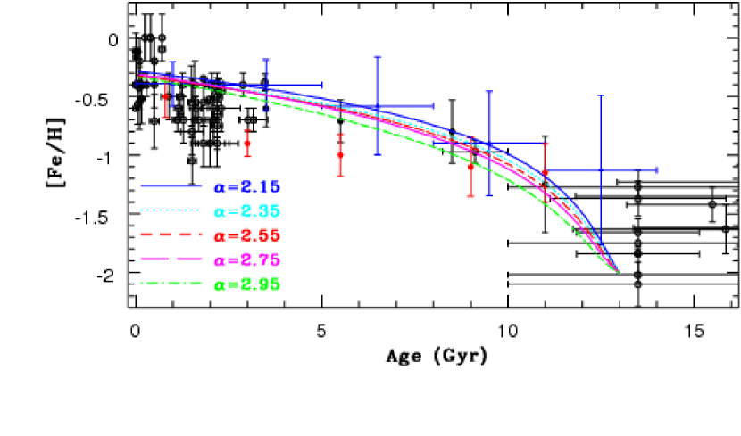
Figure 3: The AMRs for the five standard models (S1–S5) with different $\alpha$ (IMF slope): $\alpha=2.15$ (blue solid), $\alpha=2.35$ (cyan dotted), $\alpha=2.55$ (red short-dashed), $\alpha=2.75$ (magenta long-dashed), and $\alpha=2.95$ (green dot-dashed). Observational results of the LMC field stars by C05 (blue triangles), C08 (black filled circles), and HZ09 (red pentagons) are shown. The AMR for young clusters and GCs from HZ09 are also plotted by open circles.

First we describe the five standard models with different IMFs in order to demonstrate the importance of the IMF slopes in the LMC chemical evolution. In these models, $C_{\rm q}$ is chosen such that the final stellar metallicity ([Fe/H]₀) can be $-0.3$ (i.e., the observed value). Figure 3 shows the AMRs for the five models as well as the observed [Fe/H] of the LMC field stars at different age bins and and individual GCs. The AMR in each model is simply a plot of [Fe/H] at each time step (i.e., not average [Fe/H] over a given age bin like observation). Although the observational errors are not small for old GCs in the LMC, their data points are included to compare stars with the lowest [Fe/H] in the models with the corresponding observations.

The five models with no burst of star formation can reproduce reasonably well the overall trend of the observed AMR, which implies that the AMR alone can not be used for discriminating burst and non-burst models for the LMC. These models, however, appear to be less consistent with the observed [Fe/H] around ages of 2–3 Gyr (i.e., $t=$10–11 Gyr) owing to the presence of stars with significantly lower metallicities ($-1<$ [Fe/H] $<-0.5$). The models with shallower IMFs show higher [Fe/H] at a given age, which reflects the fact that chemical evolution can proceed more rapidly owing to a larger amount of metals produced by a larger number of SNe.

It should be stressed that these standard models can not reproduce so well the AMR around ages of 3–9 Gyr (i.e., $t=$4–10 Gyr) derived by HZ09 in which the AMR shows systematically lower [Fe/H] for a given age in comparison with other observations by C05 and Carrera et al. (2008, C08). The reason for this apparent difference in the observed AMRs between different observations could be related to different methods to determine ages and metallicities of stars in the observations. If the results by HZ09 are closer to the true AMR of the LMC, then the standard models with no burst can be regarded as less realistic models for the LMC evolution. Although the large [Fe/H] dispersion around an age of 2 Gyr (i.e., $t=11$ Gyr) could be simply due to star formation from gas with different metallicities (i.e., inner higher and outer lower metallicities of the LMC ISM), it could also be caused by a sudden and rapid infall of metal-poor gas from outside the LMC disk. If the observed dispersion is due to an external gas infall, then it would have profound implications for the LMC evolution. We will later discuss the implications in §4.

3.1.2 [Mg/Fe]

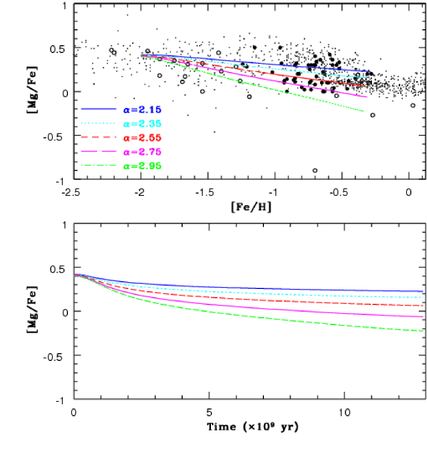
Figure 4: Chemical evolution on the LMC disk on the [Mg/Fe]-[Fe/H] plane (upper) and the time evolution of [Mg/Fe] (lower) for the five standard models (S1$-$S5) with $\alpha=2.15$ (blue solid), $\alpha=2.35$ (cyan dotted), $\alpha=2.55$ (red short-dashed), $\alpha=2.75$ (magenta long-dashed), and $\alpha=2.95$ (green dot-dashed). The observed locations of the LMC field stars (big filled circles) and clusters (big open circles) and the Galactic field stars (small dots) on the [Mg/Fe]-[Fe/H] plane are shown for comparison. The observational results include P08 for the LMC field stars, Johnson et al. 2006 (J06), Mucciarelli et al. (2008, 2010, 2011), and C12 for the LMC clusters, Gratton et al. (1999) Reddy et al. (2003) Venn et al. (2004), and Bensby et al. (2005) for the Galactic field stars.

Figure 4 shows that [Mg/Fe] slowly and monotonically decreases with time regardless of the adopted IMFs. This time-dependence of [Mg/Fe] is simply a result of a later contribution of SNIa to the chemical evolution of the LMC. The more significant decrease of [Mg/Fe] with time can be seen in the models with steeper IMFs owing to the greater contribution of SNIa to the chemical evolution in these models. The [Mg/Fe]–[Fe/H] relations do not show a plateau at low [Fe/H]. The lack of a plateau in the [Mg/Fe]–[Fe/H] relations reflects the fact that SNe Ia can chemically pollute the LMC ISM from a very early stage ($t\sim 10^{8}$ yr) of its evolution. The lack of a plateau appears to be seen in the observed [Mg/Fe]–[Fe/H] relation for [Fe/H]$<-1.5$, though it is not so clear. The [Mg/Fe]–[Fe/H] relations in the models with $\alpha\leq 2.75$ can reproduce reasonably well the overall trend of the observed [Mg/Fe] relation, though the observation shows a large [Mg/Fe] dispersion at a given [Fe/H].

The model with a very steep IMF ($\alpha=2.95$) shows systematically lower [Mg/Fe] and therefore can not reproduce so well the locations of stars in the [Mg/Fe]–[Fe/H] relation. The models with shallower IMFs show systematically larger [Mg/Fe] in the present standard models. Owing to the observed large dispersion of [Mg/Fe], it is currently difficult to determine which IMFs ($\alpha=2.35$ or 2.55 or 2.75) can better explain the observed [Mg/Fe]–[Fe/H] relation. The observed high [Mg/Fe] ($>0.4$) for higher [Fe/H] ($>-0.7$) can not be explained by any of the standard models in the present study.

3.1.3 [Ba/Fe]

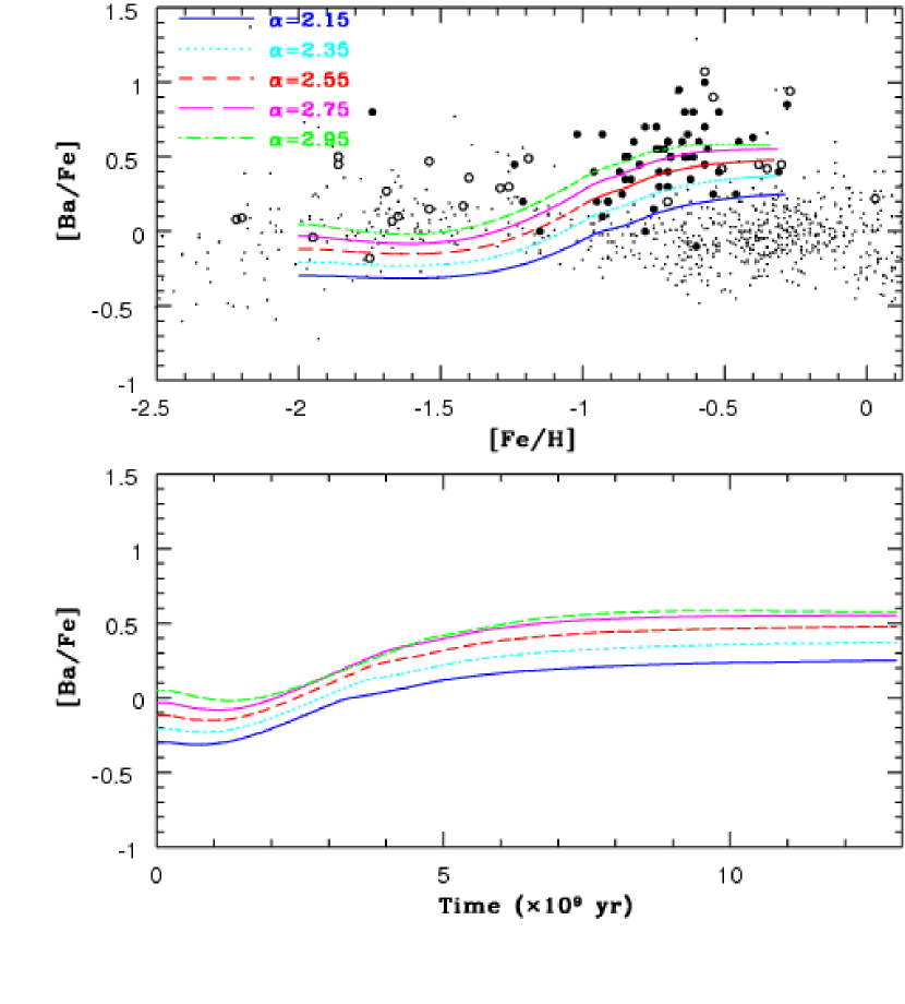
Figure 5: The same as Figure 4 but for the [Ba/Fe]–[Fe/H] relations and the [Ba/Fe] evolution.

Figure 5 shows that [Ba/Fe] starts to slowly increase with time about 2 Gyr after the commencement of active star formation in the LMC disk. This slow [Ba/Fe] increase is due to the ejection of $s-$process elements from low-mass ($<3M_{\odot}$) AGB stars. The observed systematically high [Ba/Fe] ($>0$ for most stars) at [Fe/H] $<-1.5$ seems to be better reproduced by the models with steeper IMFs, though the very high [Ba/Fe] ($>0.2$) in some stars at such low metallicities can not be reproduced at all by any of the standard models in the present study. The reason for the higher [Ba/Fe] at [Fe/H]$<-1$ in steeper IMFs is that the numerical ratio of SNe II with masses of $\sim 8M_{\odot}$ to those with $\sim 10M_{\odot}$ (and thus the contribution of these SNe to the chemical evolution) can change in the steeper IMF and consequently [Ba/Fe] can increase more significantly in the early history of the chemical evolution of the LMC. The maximum [Ba/Fe] in the model with the Salpeter IMF is at most [Ba/Fe]$\sim 0.4$, whereas most of the LMC stars at [Fe/H]$>-0.6$ show [Ba/Fe]$\geq 0.4$. These results strongly suggest that the LMC could have had a steeper IMF (at least steeper than the Salpeter IMF with $\alpha=2.35$) in its star formation history (if the LMC has not experienced starbursts). The observed very high [Ba/Fe] ($>0.8$) of some stars at [Fe/H]$\sim-0.6$ can not be explained at all by any of the standard models in the present study.

3.1.4 $f_{\rm g}$-[Fe/H] relation

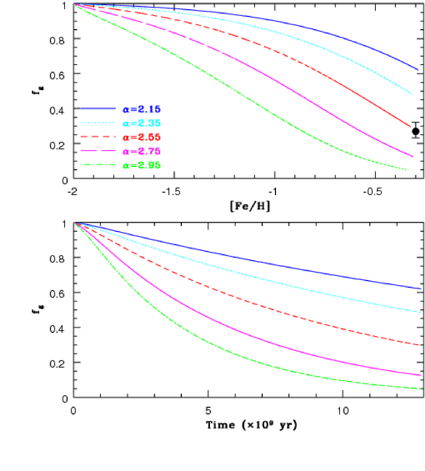
Figure 6: The same as Figure 4 but for the $f_{\rm g}$–[Fe/H] relations and the $f_{\rm g}$ evolution. The filled circle with a vertical error bar indicates the observed present gas mass fraction of the LMC ($f_{\rm g,0}$).

In the present study, the $C_{\rm q}$ for each model is chosen such that the final [Fe/H] (i.e., [Fe/H]₀) is consistent with the observed one ($-0.3$). A smaller amount of metals can be ejected from SNe in the models with steeper IMFs owing to the smaller numbers of SNe. Therefore, ISM in the models with steeper IMFs needs to be more rapidly consumed by star formation and chemically enriched by SN ejecta to reach [Fe/H]${}_{0}=-0.3$. Figure 6 shows that (i) the models with steeper IMFs show smaller $f_{\rm g,0}$ and (ii) the model with $\alpha=2.55$ is the most consistent with the observed $f_{\rm g,0}$. These results suggest that the observed $f_{\rm g,0}$ and [Fe/H]₀ combine to support the steeper IMF ($\alpha\approx 2.55$) of the LMC. However this suggestion depends on the adopted assumption that no ISM can be expelled from the LMC in the standard models. If a significant fraction of cold ISM can be stripped from the LMC, even the models with shallower IMFs (e.g., $\alpha=2.15$) may be able to explain both $f_{\rm g,0}$ and [Fe/H]₀. Likewise, if a significant fraction of cold ISM can be recently accreted onto the LMC, the models with rather steep IMFs (e.g., $\alpha>2.75$) may explain both $f_{\rm g,0}$ and [Fe/H]₀ too.

3.2 Burst models

3.2.1 AMR

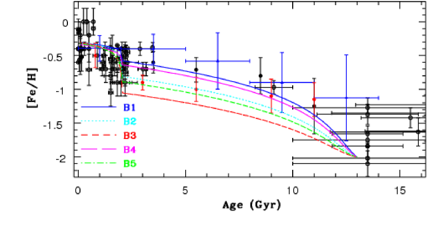
Figure 7: The same as Figure 3 but for the five burst models, B1 with $\alpha=2.35$ and $C_{\rm q}=0.004$ (blue solid), B2 with $\alpha=2.55$ and $C_{\rm q}=0.004$ (cyan dotted), B3 with $\alpha=2.75$ and $C_{\rm q}=0.004$ (red short-dashed), B4 with $\alpha=2.55$ and $C_{\rm q}=0.006$ (magenta long-dashed), and B5 with $\alpha=2.75$ and $C_{\rm q}=0.006$ (green dot-dashed). The parameter $C_{\rm q}$ can control the rapidity of star formation in the quiescent phase before starburst (see the main text for more details of $C_{\rm q}$).

The burst of star formation and the subsequent efficient production of metals can rapidly and significantly increase [Fe/H] in the burst models. Therefore, the chemical evolution in the quiescent phase of star formation in the burst models needs to proceed more slowly (i.e., smaller $C_{\rm q}$) in comparison with the standard models so that the final [Fe/H] can be as low as $-0.3$. Figure 7 shows the AMRs in the five burst models with different IMFs and $C_{\rm q}$. The burst model B3 can not reproduce the observed AMR owing to the systematically low [Fe/H] in the quiescent phase of star formation. The model B1 with the Salpeter IMF can better explain the AMR of C05 and C08 whereas the models with steeper IMFs (B2 and B5) can explain better the AMR by HZ09. The observed AMR thus cannot give strong constraints on the IMF of the LMC. Owing to the observed large [Fe/H] dispersion at an age of $\sim 2$ Gyr ($t=11$ Gyr), the AMR alone can not allow us to make a robust conclusion as to whether the LMC experienced a burst of star formation at an age of 2 Gyr (i.e., $t=11$ Gyr).

3.2.2 [Mg/Fe]

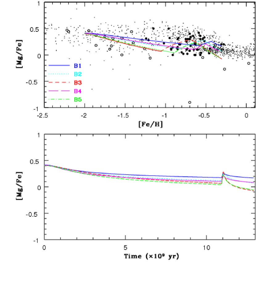
Figure 8: The same as Figure 4 but for the five burst models, B1 with $\alpha=2.35$ and $C_{\rm q}=0.004$ (blue solid), B2 with $\alpha=2.55$ and $C_{\rm q}=0.004$ (cyan dotted), B3 with $\alpha=2.75$ and $C_{\rm q}=0.004$(red short-dashed), B4 with $\alpha=2.55$ and $C_{\rm q}=0.006$ (magenta long-dashed), and B5 with $\alpha=2.75$ and $C_{\rm q}=0.006$ (green dot-dashed).

As shown in Figure 8, the overall trends of the [Mg/Fe] evolution in the quiescent phase for the burst models are similar to those for the standard ones. The [Mg/Fe]–[Fe/H] relations in the burst models show “bumps” (a sharp increase followed by a decrease in the time evolution of [Mg/Fe]) whose magnitudes depend on $C_{\rm s1}$ and $\alpha$. The observed locations of the LMC stars in the [Mg/Fe]-[Fe/H] plane do not show clearly such a bump. However, if the two stars with [Mg/Fe]$\sim 0.5$ at [Fe/H]$\sim-1.2$ and $-1.0$ are removed from Figure 8, then the remaining stars appear to show a bump around $-0.7<$[Fe/H]$<-0.6$. Furthermore, the apparent lack of stars with [Mg/Fe]$>0.3$ at [Fe/H]$\sim-0.4$ suggests that [Mg/Fe] has been decreasing since [Fe/H]$=-0.5$. Thus the higher [Mg/Fe] at [Fe/H]$\sim-0.6$ could be evidence of a starburst around $t=11$ Gyr (i.e., 2 Gyr ago). However, the observed [Mg/Fe] dispersion at [Fe/H]$\sim-0.6$ is so large that we can not make a robust conclusion as to whether a starburst occurred in the LMC about $t=11$ Gyr (i.e., 2 Gyr ago). Also it should be noted that the smaller number of stars at [Fe/H]$>-0.5$ could be responsible for the apparent lack of stars with higher ($>0.3$) [Mg/Fe].

3.2.3 [Ba/Fe]

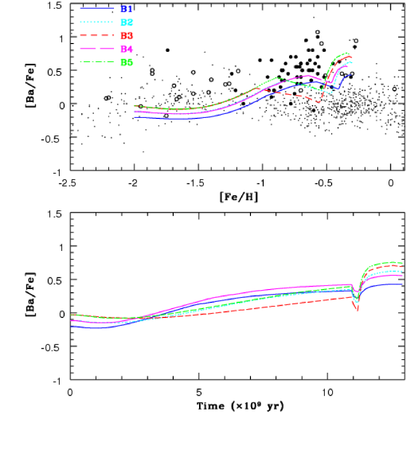
Figure 9: The same as Figure 5 but for the five burst models, B1 with $\alpha=2.35$ and $C_{\rm q}=0.004$ (blue solid), B2 with $\alpha=2.55$ and $C_{\rm q}=0.004$ (cyan dotted), B3 with $\alpha=2.75$ and $C_{\rm q}=0.004$(red short-dashed), B4 with $\alpha=2.55$ and $C_{\rm q}=0.006$ (magenta long-dashed), and B5 with $\alpha=2.75$ and $C_{\rm q}=0.006$ (green dot-dashed).

Figure 9 shows that irrespective of the model parameters, [Ba/Fe] rapidly decreases soon after the starbursts owing to the ejection of Fe-rich gas from prompt SNe Ia in the time evolution of [Ba/Fe]. The temporary [Ba/Fe] decrease is subsequently followed by its rapid and sharp increase due to chemical pollution by AGB ejecta. Owing to the rapid [Ba/Fe] increase, the burst models can show systematically higher final [Ba/Fe] in comparison with the standard models with no burst. Therefore, the observed presence of stars with higher [Ba/Fe] ($>0.5$) at [Fe/H]$\approx-0.3$ could be more consistent with the burst models. The burst models with steeper IMFs ($\alpha=2.75$) show [Ba/Fe]$\sim 0.7$ at [Fe/H]$=-0.3$, which suggests that the combination of a steeper IMF and a secondary starburst could be closely associated with the origin of stars with [Ba/Fe] as large as 0.7. However, very high [Ba/Fe] ($>0.9$) at [Fe/H]$\sim-0.6$ can not be explained by the present starburst models. These stars with very high [Ba/Fe] could have been formed directly from AGB ejecta that did not mix well with the ISM.

3.2.4 $f_{\rm g}$–[Fe/H] relation

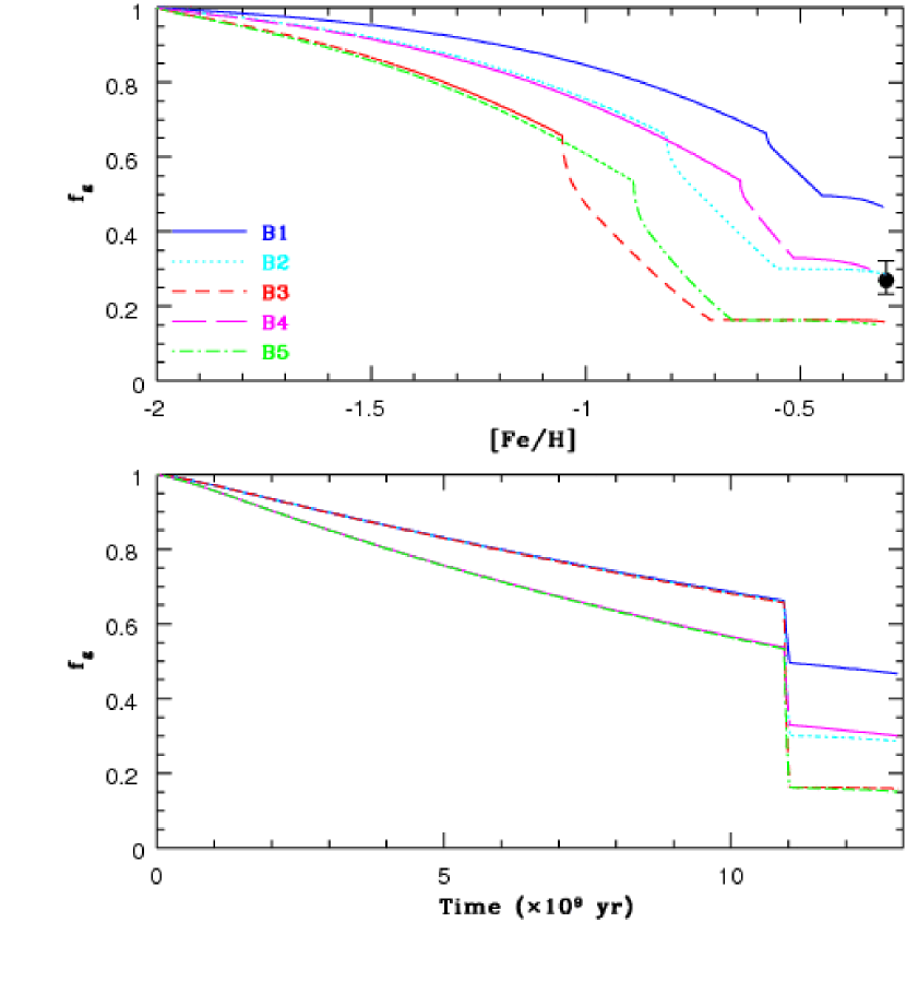
Figure 10: The same as Figure 6 but for the five burst models, B1 with $\alpha=2.35$ and $C_{\rm q}=0.004$ (blue solid), B2 with $\alpha=2.55$ and $C_{\rm q}=0.004$ (cyan dotted), B3 with $\alpha=2.75$ and $C_{\rm q}=0.004$(red short-dashed), B4 with $\alpha=2.55$ and $C_{\rm q}=0.006$ (magenta long-dashed), and B5 with $\alpha=2.75$ and $C_{\rm q}=0.006$ (green dot-dashed).

Figure 10 clearly shows that the burst model with the Salpeter IMF can not reproduce simultaneously the observed $f_{\rm g,0}$ and [Fe/H]₀ owing to efficient chemical enrichment. On the other hand, a larger amount of gas needs to be consumed for the ISM to be chemically enriched to [Fe/H]$\sim-0.3$ in the models with steep IMFs ($\alpha=2.75$) so that $f_{\rm g,0}$ can become significantly smaller in the model. The models with $\alpha=2.55$ yet different star formation histories in the quiescent phases can best reproduce both the observed $f_{\rm g,0}$ and [Fe/H]₀. These results on the IMF-dependences are essentially the same as those derived for the standard model.

3.3 Double-burst models

3.3.1 AMR

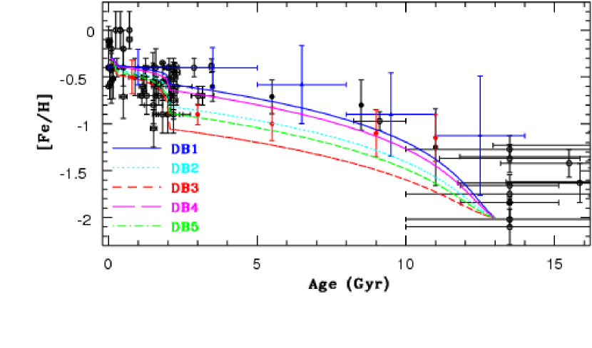
Figure 11: The same as Figure 3 but for the five double-burst models, DB1 with $\alpha=2.35$ and $C_{\rm q}=0.004$ (blue solid), DB2 with $\alpha=2.55$ and $C_{\rm q}=0.004$ (cyan dotted), DB3 with $\alpha=2.75$ and $C_{\rm q}=0.004$(red short-dashed), DB4 with $\alpha=2.55$ and $C_{\rm q}=0.006$ (magenta long-dashed), and DB5 with $\alpha=2.75$ and $C_{\rm q}=0.006$ (green dot-dashed). The strength of the starbursts ($C_{\rm sb1}$ and $C_{\rm sb2}$) at 2 Gyr ago and 0.2 Gyr ago ($t_{\rm sb1,s}\leq t\leq t_{\rm sb1,e}$ and $t_{\rm sb2,s}\leq t\leq t_{\rm sb2,e}$) at each model are chosen such that the final [Fe/H] is the same as the observed one (i.e., $-0.3$). The parameters $t_{\rm sb1,s}$ and $t_{\rm sb1,e}$ ($t_{\rm sb2,s}$ and $t_{\rm sb2,e}$) can control the start and the end of the first (second) starburst, respectively, in the LMC.

Figure 11 shows the dependences of the AMRs on IMFs and star formation histories in the quiescent phase for the double-burst models. The derived IMF dependence of AMRs are very similar to those in the burst ones. The model DB3 with steep IMF ($\alpha=2.75$) and less rapid star formation in the quiescent phase is inconsistent with any observational results on the AMR. The model DB1 with the Salpeter IMF can better reproduce the observed AMRs of C05 and C08 whereas the model DB2 with moderately steep IMF ($\alpha=2.55$) can be better fit to the AMR by H09. Although the burst at $t=12.8$ Gyr is as strong as that at $t=11$ Gyr, the signature of the burst in the AMR is less clear in the double-burst models. The observed AMR shows a large [Fe/H] dispersion in the youngest stellar population (i.e., [Fe/H] ranging from $\sim-0.6$ to $\sim 0$), and the presence of such relatively metal-poor ([Fe/H]$\sim-0.6$) stars at the present time is puzzling. The recent accretion of metal-poor gas and the resultant active star formation (before the burst at $t=12.8$ Gyr) could result in the formation of such metal-poor stars and thus introduce a larger scatter in [Fe/H] at the young populations.

3.3.2 [Mg/Fe]

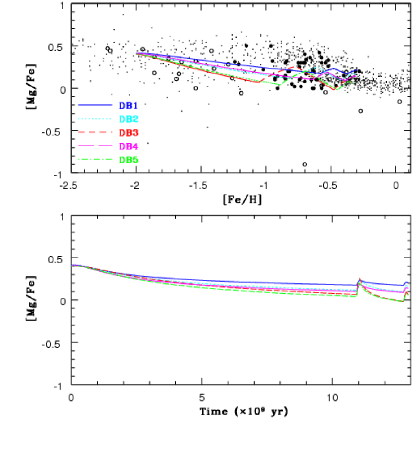
Figure 12: The same as Figure 4 but for the five double-burst models, DB1 with $\alpha=2.35$ and $C_{\rm q}=0.004$ (blue solid), DB2 with $\alpha=2.55$ and $C_{\rm q}=0.004$ (cyan dotted), DB3 with $\alpha=2.75$ and $C_{\rm q}=0.004$(red short-dashed), DB4 with $\alpha=2.55$ and $C_{\rm q}=0.006$ (magenta long-dashed), and DB5 with $\alpha=2.75$ and $C_{\rm q}=0.006$ (green dot-dashed).

Figure 12 shows that the time evolution of [Mg/Fe] in the double-burst models is characterized by two occurrences of sharp [Mg/Fe] increase/decrease after starbursts, which result in two bumps. The double-burst models show two bumps in the [Mg/Fe]-[Fe/H] plane, though such bumps are not clearly seen in the observations. The final [Mg/Fe] is larger than 0 for all double-burst models owing to the last starburst at $t=12.8$ Gyr, which is a feature that discriminates between the burst and double-burst models. The models (DB3, 4 and 5) with steeper IMFs show smaller final [Mg/Fe] and the final [Mg/Fe] in the model DB1 with $\alpha=2.35$ is more consistent with the observed one for the LMC field stars. The observed [Mg/Fe] of the field stars with $-0.5<$[Fe/H]$<-0.3$ appears to increase from $\sim 0$ to $0.2$, which may be regarded as the second bump due to the starburst at $t=12.8$ Gyr. The second bump can be shown more clearly in the models DB3 and DB5 with steeper IMFs ($\alpha=2.75$). As noted in §3.2, the observed large [Mg/Fe] dispersion at a given [Fe/H] makes it difficult for us to confirm the presence (or absence) of the first and second starbursts in the observed [Mg/Fe]–[Fe/H] relation.

3.3.3 [Ba/Fe]

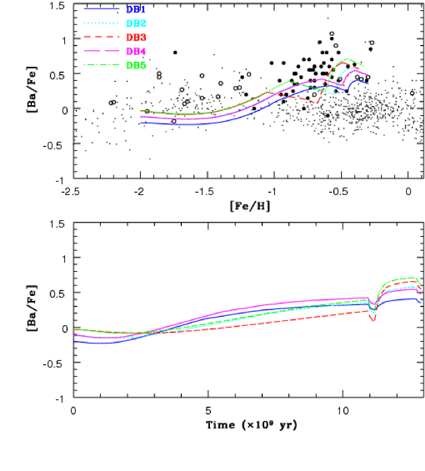
Figure 13: The same as Figure 5 but for the five double-burst models, DB1 with $\alpha=2.35$ and $C_{\rm q}=0.004$ (blue solid), DB2 with $\alpha=2.55$ and $C_{\rm q}=0.004$ (cyan dotted), DB3 with $\alpha=2.75$ and $C_{\rm q}=0.004$(red short-dashed), DB4 with $\alpha=2.55$ and $C_{\rm q}=0.006$ (magenta long-dashed), and DB5 with $\alpha=2.75$ and $C_{\rm q}=0.006$ (green dot-dashed).

Figure 13 shows that [Ba/Fe] rapidly decreases soon after the first starburst at $t=11$ Gyr and then increases until the commencement of the second starburst at $t=12.8$ Gyr for the double-burst models with different IMFs (in the time evolution of [Ba/Fe]). The increase of [Ba/Fe] after the second starburst can not be seen, because the 0.2 Gyr difference between the present and the last starburst is not long enough for AGB stars to have chemically polluted the LMC ISM. Owing to the first starburst, [Ba/Fe] can become significantly high (up to $\sim 0.7$) in the double-burst models. However, the maximum value across all models is still significantly lower than those ($>0.9$) observed in some stars with [Fe/H]$=-0.6\sim-0.5$. The models with steeper IMFs can show higher final [Ba/Fe] and they can better explain the clear differences in the locations of field stars in the [Ba/Fe]-[Fe/H] plane between the LMC and the Galaxy.

3.3.4 $f_{\rm g}$–[Fe/H] relation

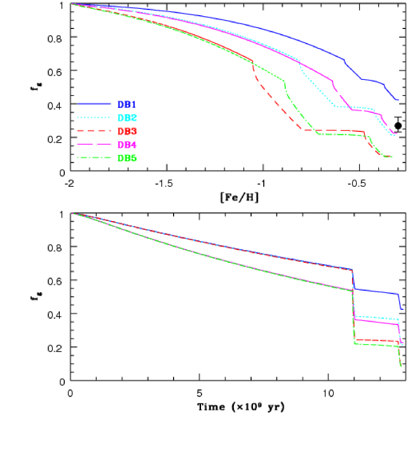
Figure 14: The same as Figure 6 but for the five double-burst models, DB1 with $\alpha=2.35$ and $C_{\rm q}=0.004$ (blue solid), DB2 with $\alpha=2.55$ and $C_{\rm q}=0.004$ (cyan dotted), DB3 with $\alpha=2.75$ and $C_{\rm q}=0.004$(red short-dashed), DB4 with $\alpha=2.55$ and $C_{\rm q}=0.006$ (magenta long-dashed), and DB5 with $\alpha=2.75$ and $C_{\rm q}=0.006$ (green dot-dashed).

Figure 14 shows that the best model to explain both $f_{\rm g,0}$ and [Fe/H]₀ simultaneously is the one with $\alpha=2.55$ among the double-burst models (i.e., DB2 and DB4). This result combined with those in the standard and burst models strongly suggests that the IMF of the LMC should be moderately steeper ($\alpha\approx 2.55$) in its long-term star formation history. As demonstrated, the models with steeper IMF can better explain the presence of the LMC field stars with [Ba/Fe]$>0.5$ and higher [Ba/Fe] of GCs at low metallicities ([Fe/H]$<-1.5$). It should be noted here that all ejecta from AGB stars and SNe are retained in the LMC for these non-wind models. Thus, it can be concluded that a steeper IMF ($\alpha\sim 2.55$) can better explain the star formation and chemical evolution histories of the LMC, as long as the LMC has not lost a significant amount of its chemically enriched ISM through stellar winds.

3.4 Wind models

3.4.1 AMR

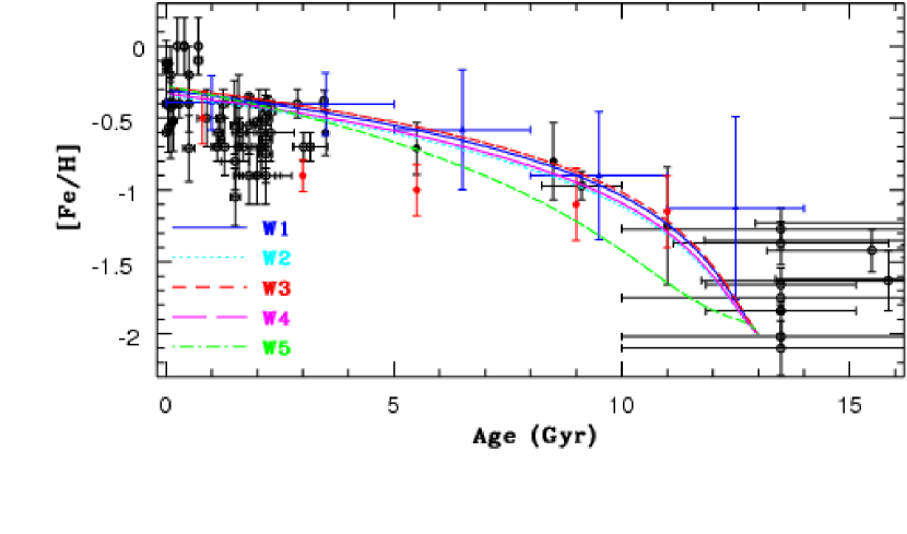
Figure 15: The same as Figure 3 but for the five wind models, W1 with $\alpha=2.35$ and $f_{\rm ej}=0.4$ (blue solid), W2 with $\alpha=2.55$ and $f_{\rm ej}=0.4$ (cyan dotted), W3 with $\alpha=2.35$ and $f_{\rm ej}=0.2$(red short-dashed), W4 with $\alpha=2.55$ and $f_{\rm ej}=0.2$ (magenta long-dashed), and W5 with $\alpha=2.35$ and $C_{\rm ej}=300$ (green dot-dashed). C1–C4 are selective wind models whereas C5 is a non-selective wind model. Starbursts do not occur in these wind models.

Figure 15 shows that (i) the AMRs are not so different between selective wind models (W1$-$W4) with different $\alpha$, $C_{\rm q}$, and $f_{\rm ej}$ and (ii) chemical evolution proceeds significantly more slowly in the non-selective wind model (W5) than in the selective ones until recently ($t\sim 8$ Gyr) so that the AMR in the non-selective wind model shows systematically lower [Fe/H] for a given age. Although the non-selective wind model can explain the observed [Fe/H]₀, the total gas mass ejected from the LMC ($M_{\rm ej,t}$) for 13 Gyr is about 3.4 times larger than the final stellar mass (i.e., $M_{\rm ej,t}=9.1\times 10^{9}M_{\odot}$ for $M_{\rm s}=2.7\times 10^{9}{\rm M}_{\odot}$) and thus appears to be too large. Both already existing ISM and newly synthesized metals can be efficiently removed from the LMC in the non-selective wind models so that the chemical evolution of the LMC can proceed much more slowly. As a result of this, a much larger amount of gas can be removed from the LMC until the stellar metallicity finally becomes [Fe/H]$\approx 0.3$ in the non-selective wind model (W5). The AMRs in the selective wind models are very similar to the standard models: They are more consistent with the observed one by C05 and C08 than that by HZ09. This result implies that the observed AMR alone does not enable us to discuss the effects of stellar winds in the LMC chemical evolution.

3.4.2 [Mg/Fe]

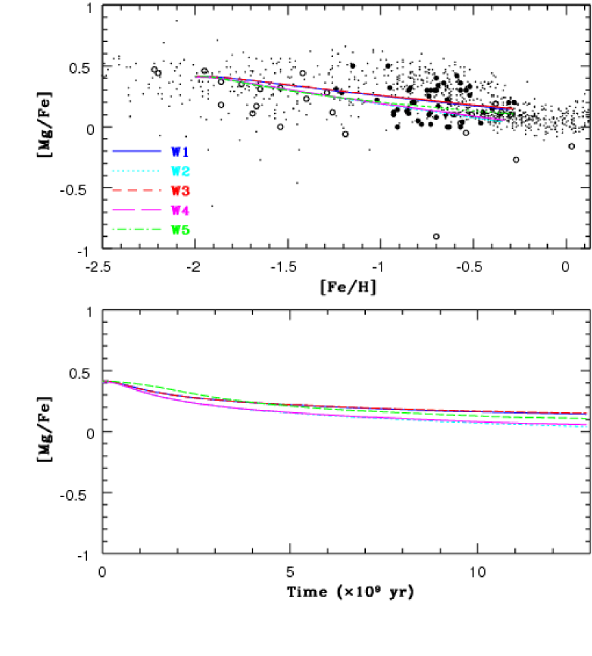
Figure 16: The same as Figure 4 but for the five wind models, W1 with $\alpha=2.35$ and $f_{\rm ej}=0.4$ (blue solid), W2 with $\alpha=2.55$ and $f_{\rm ej}=0.4$ (cyan dotted), W3 with $\alpha=2.35$ and $f_{\rm ej}=0.2$(red short-dashed), W4 with $\alpha=2.55$ and $f_{\rm ej}=0.2$ (magenta long-dashed), and W5 with $\alpha=2.35$ and $C_{\rm ej}=300$ (green dot-dashed).

Figure 16 shows that the monolithic decrease of [Mg/Fe] with time and the [Mg/Fe]–[Fe/H] relation in the five wind models are essentially similar to those derived in the standard models with no wind. The selective wind models with larger $f_{\rm ej}$ show slightly higher [Mg/Fe] for a given IMF whereas those with steeper IMFs show lower [Mg/Fe] for a given $f_{\rm ej}$. The five wind models can not explain the observed higher [Mg/Fe] ($>0.2$) for [Fe/H] $>-0.6$ in the LMC field stars. There is no remarkable difference in the [Mg/Fe] evolution between the selective and non-selective wind models.

3.4.3 [Ba/Fe]

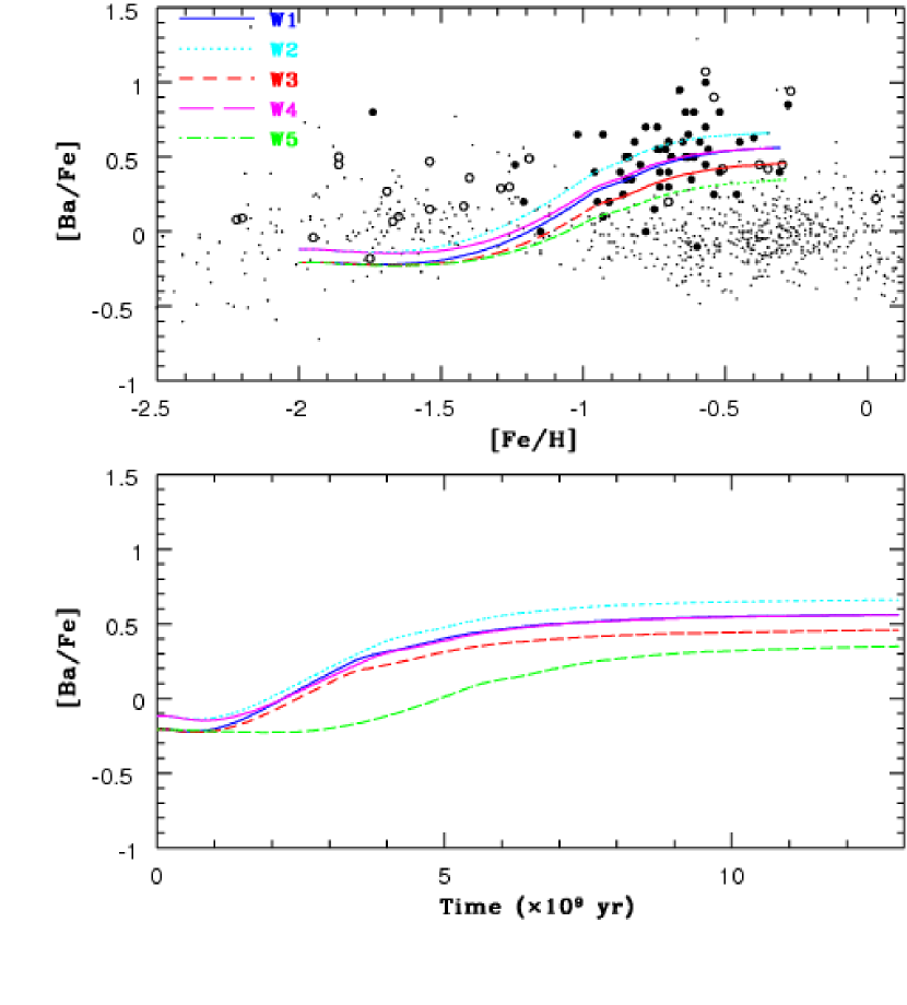
Figure 17: The same as Figure 5 but for the five wind models, W1 with $\alpha=2.35$ and $f_{\rm ej}=0.4$ (blue solid), W2 with $\alpha=2.55$ and $f_{\rm ej}=0.4$ (cyan dotted), W3 with $\alpha=2.35$ and $f_{\rm ej}=0.2$(red short-dashed), W4 with $\alpha=2.55$ and $f_{\rm ej}=0.2$ (magenta long-dashed), and W5 with $\alpha=2.35$ and $C_{\rm ej}=300$ (green dot-dashed).

Figure 17 shows that the selective wind models can show higher [Ba/Fe] ($>0.5$) for [Fe/H]$>-0.6$ for a range of $\alpha$ and $f_{\rm ej}$. The model W2 with $\alpha=2.55$ and $f_{\rm ej}=0.4$ shows [Ba/Fe]$>0.6$ without secondary starbursts, because Fe-rich gas is ejected from the LMC disk whereas the AGB ejecta containing $s$-process elements (e.g., Ba) can be retained and thus used for chemical evolution. These results imply that efficient removal of SNe ejecta from the LMC disk is a way to significantly increase [Ba/Fe] without starburst(s). The models with steeper IMFs show higher [Ba/Fe], which is essentially the same as the results derived for the standard models. The final (thus maximum) [Ba/Fe] in the non-selective wind model at [Fe/H] $=-0.3$ is lower than 0.4, and therefore inconsistent with the observed value, which implies that the non-selective wind model is less promising than the selective wind one as a reasonable model for LMC chemical evolution.

3.4.4 $f_{\rm g}$–[Fe/H] relation

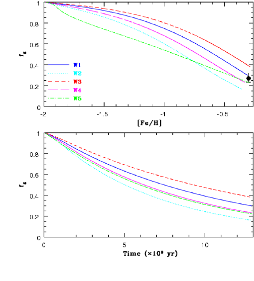
Figure 18: The same as Figure 6 but for the five wind models, W1 with $\alpha=2.35$ and $f_{\rm ej}=0.4$ (blue solid), W2 with $\alpha=2.55$ and $f_{\rm ej}=0.4$ (cyan dotted), W3 with $\alpha=2.35$ and $f_{\rm ej}=0.2$(red short-dashed), W4 with $\alpha=2.55$ and $f_{\rm ej}=0.2$ (magenta long-dashed), and W5 with $\alpha=2.35$ and $C_{\rm ej}=300$ (green dot-dashed).

Figure 18 shows that the selective wind model W1 with the Salpeter IMF appears to better fit the observed $f_{\rm g,0}$ and [Fe/H]₀ than the models with steeper IMF ($\alpha=2.55$) for $f_{\rm ej}=0.4$ (W2). However, the model with steeper IMF and $f_{\rm ej}=0.2$ (W4) can also better explain the observed two quantities than that with the Salpeter IMF and $f_{\rm ej}=0.2$ (W3): it should be noted that the model W5 can also explain $f_{\rm g,0}$ but does not show the observed high [Ba/Fe] at [Fe/H]$\sim-0.6$. These results mean that if we carefully choose the two parameters ($\alpha$ and $f_{\rm ej}$), the observation can be well reproduced. The non-selective wind model with the Salpeter IMF can also reproduce both $f_{\rm g,0}$ and [Fe/H]₀ reasonably well. We do not intend to discuss the wind models with starburst(s), because the effects of starbursts on the LMC chemical evolution are essentially the same as those already described in the burst and double-burst models.

3.5 Comparison between the four different types of models

We here briefly summarize the advantages and disadvantages of the four different types of models in reproducing recent observational results (see Table 2 for a brief summary). The observed AMR can be consistent with most models with a reasonable set of model parameters. The models with steeper IMFs ($\alpha\geq 2.55$) can better explain the observed $f_{\rm g,0}$–[Fe/H] relation and [Ba/Fe]$>-0.2$ at [Fe/H]$>-1.5$ in a self-consistent manner. The apparent bump in the observed [Mg/Fe]–[Fe/H] relation at [Fe/H]$\sim-0.6$ can be better reproduced in models with starbursts. The higher [Ba/Fe] $\sim 0.5$ at [Fe/H]$\sim-0.3$ can be better explained by non-starburst models (i.e., standard ones) with steeper IMFs and starburst ones. Very high [Ba/Fe] ($>0.9$) at [Fe/H]$\sim-0.6$ can not be explained by any of the models in the present study. The significantly higher ($>0.2$) [Ba/Fe] observed in some old, metal-poor GCs ([Fe/H]$<-1.5$) can not be explained by any of these models, either.

The selective wind models with the Salpeter IMF can better explain observations than the non-wind models with the Salpeter IMF, though the selective wind models need to assume an apparently large $f_{\rm ej}=0.4$ and can not accurately reproduce the [Ba/Fe] of the stars in the metal-poor GCs with [Fe/H]$<-1.5$. This leads us to suggest that a steeper IMF is required for explaining the different observed chemical properties of the LMC in a self-consistent manner. The removal of metals from SNe can also significantly increase the [Ba/Fe] (up to $\sim 0.8$) after a starburst if a large $f_{\rm ej}>0.5$ is chosen in the selective wind models. This implies that the selective removal of SNe ejecta could be partly responsible for the observed rather high [Ba/Fe] ($\sim 0.8$) in the LMC field stars. Thus, there are two possible ways to explain the high [Ba/Fe]: One is star formation directly from Ba-rich AGB ejecta and the other is significantly efficient selective removal of SN ejecta.

Thus, as summarized in Table 2, the four different types of models can explain most of the observed chemical properties of the LMC reasonably well (except the unusually high [Ba/Fe]), as long as the model parameters are carefully chosen. The observed AMR and overall trends of the [Mg/Fe]–[Fe/H] (and equally the [$\alpha$/Fe]–[Fe/H]) and the [Ba/Fe]–[Fe/H] relations can give less strong constraints on the IMF and the star formation history of the LMC. Table 3 describes how the four key chemical properties of the LMC constrain the IMF and the presence or absence of past starbursts.

4 Discussion

4.1 A steeper IMF?

The present study has shown that the standard, burst, and double-burst models with steeper IMFs ($\alpha\sim 2.55$) can explain well the observed $f_{\rm g}$ and [Fe/H]₀ in a self-consistent manner. Furthermore such non-wind models can not only better explain the observed higher [Ba/Fe] at [Fe/H]$<-1.5$ in the LMC (due to the steeper IMFs which raise the $r$-process/Fe ratio), but also can reproduce well the overall dependence of [Ba/Fe] on [Fe/H]. Although the selective wind models with the Salpeter IMFs ($\alpha=2.35$) can explain both $f_{\rm g}$ and [Fe/H]₀ in a self-consistent manner for a larger $f_{\rm ej}$ ($\sim 0.4$), they can not explain so well the observed [Ba/Fe] at [Fe/H]$\sim-1.5$. Therefore, the non-wind models with steeper IMFs seems to be slightly better models for the adopted stellar yields.

Although it seems to be premature to observationally determine whether the IMF of the LMC is clearly steeper than the Salpeter one, a number of previous observations have suggested a steeper IMF in the LMC. For example, Mateo (1988) investigated the IMFs of stars with masses ranging from $0.9M_{\odot}$ to $10.5M_{\odot}$ in the six clusters of the LMC and found that the slopes are typically $\alpha\sim 3.5$. Hill et al. (1994) also found a steeper IMF ($\alpha\sim 3$) for young stars with masses larger than $9M_{\odot}$ in the LMC and also suggested that the IMF can be different below and above $9M_{\odot}$. Holtzman et al. (1997) investigated the IMF for stars on the main sequence which are fainter than the oldest turnoff and discussed the possibility of a steep IMF with $\alpha=2.75$ for the LMC dominated by young populations. As shown in Figures 4 and 6 of this paper, rather steep IMFs (e.g., $\alpha\geq 2.95$) cannot be consistent with the observed chemical properties and AMR of the LMC.

The only difference in the non-wind models with steeper IMFs and the selective wind ones with the Salpeter ones is the [Fe/H]-dependence of [Ba/Fe] at lower [Fe/H] ($<-1.5$). Most of the observed field stars and GCs with [Fe/H]$<-1.5$ in the LMC show [Ba/Fe]$>-0.2$, which is more consistent with the non-wind models with steeper IMFs. However the total number of data points in the observed [Ba/Fe]–[Fe/H] diagram is sufficiently small that we can not make a robust conclusion as to whether the non-wind models or the selective wind ones are better in explaining the observed [Ba/Fe] trend with [Fe/H]. Thus it is undoubtedly worthwhile for future spectroscopic observations to investigate [Ba/Fe] and other $s$-process elements of the metal-poor stellar populations of the LMC with [Fe/H]$<-1.5$ to obtain better constraints on the IMF and the ejection processes of SN ejecta in the LMC.

4.2 Evidence for prompt SNe Ia and jet-induced SNe II?

The present study first investigated how a prompt SNe Ia influences the chemical evolution of the LMC and thereby predicted that [$\alpha$/Fe] decreases monotonically (until a secondary starburst occurs) with no remarkable plateau in the [$\alpha$/Fe]–[Fe/H] relation for low [Fe/H]. We should first investigate [Mg/Fe]–[Fe/H] relations, firstly because this element is most reliably determined by the observations among $\alpha$-elements, and secondly because its yield is most reliably predicted by nucleosynthesis calculations. The second best $\alpha$-element for this investigation is Ca. On the other hand, Ti and Si are not so good since Ti is not well predicted by SN II nucleosynthesis, and the observed determination of the Si abundance involves a large uncertainty.

The observed [Mg/Fe]–[Fe/H] relation does not show the predicted trends so clearly partly because of the large dispersion in [Mg/Fe] at each [Fe/H]. Although the physical reasons for the large [Mg/Fe] dispersion are not so clear, one of the posssible explanations is described as follows. If different local regions have different star formation histories (e.g., due to different local gas densities and gas infall rates) in the LMC, as observed in recent observations (e.g., HZ09 and R12), then they can have different [Mg/Fe] owing to different chemical enrichment histories. Therefore, the observed large scatter can be due to different evolutions of [Mg/Fe] in different local regions of the LMC.

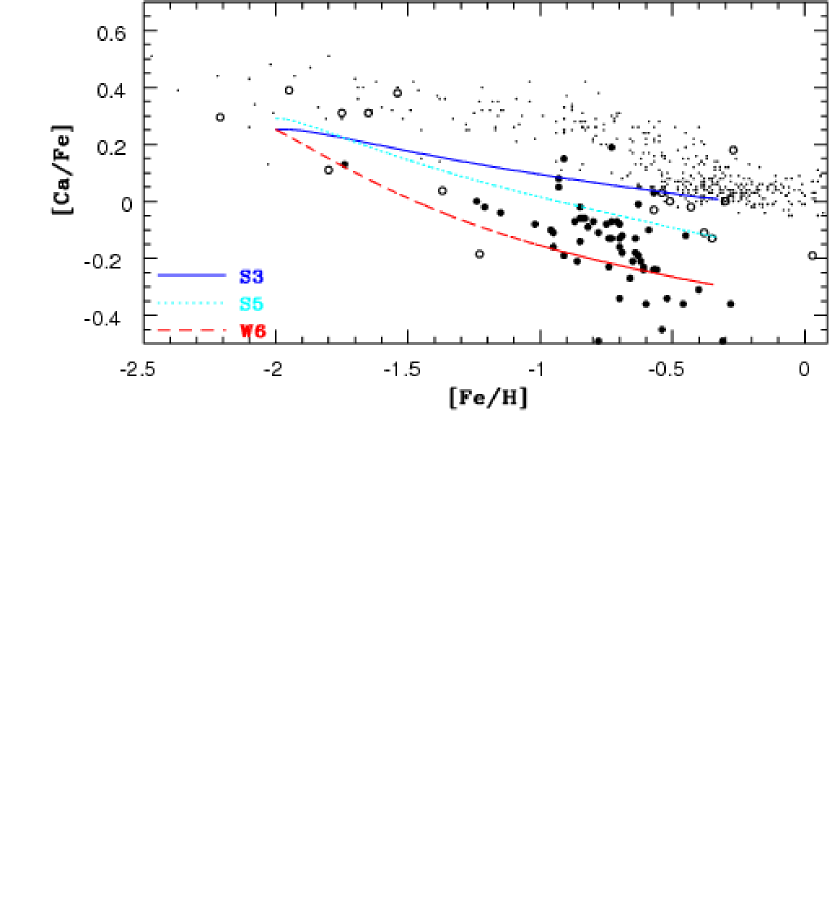
Figure 19: Chemical evolution on the [Ca/Fe]-[Fe/H] plane for the three models S3 (blue solid), S5 (cyan dotted), and W6 (red dashed). The observational plots are from observational studies shown in Figure 4. The wind model W6 is different from other wind models in that Ca can be by a factor of 1.7 more efficiently removed from the LMC disk in comparison with other elements from SNe. This selective removal of Ca is based on previous theoretical studies on nucleosynthesis of jet-induced SNe (Shigeyama et al. 2010). Note that the wind model W6 can be better fit to the observed low [Ca/Fe] ($<-0.2$) for the LMC field stars with [Fe/H]$>-1.0$.

The observed [Ca/Fe]–[Fe/H] relation can be also used for discussing whether there is evidence for the prompt SNe Ia playing a significant role in the chemical evolution of the LMC. Figure 19 shows the locations of the LMC stars on the [Ca/Fe]-[Fe/H] plane as well as the predicted [Ca/Fe]–[Fe/H] relations for three different models. These three models are chosen because they, in combination, show widely different [Ca/Fe]–[Fe/H] relations of the LMC stars. It is clear that [Ca/Fe] decreases as [Fe/H] increases without showing a clear plateau for [Fe/H]$<-1$ in the LMC stars, which is consistent with the predictions of the present models with prompt SNe Ia. In addition, the observed locations of the LMC stars on the [Ti/Fe]-[Fe/H] plane clearly show a trend for a wide range of metallicity similar to [Ca/Fe] (e.g., C12). However the [Si/Fe]–[Fe/H] relation does not show such a clear trend owing to a larger [Si/Fe] dispersion for stars with [Fe/H]$<-1.5$ (e.g., Figure 4 in C12). These results on the [Ca/Fe]–[Fe/H] and [Ti/Fe]–[Fe/H] relations are supporting evidence that prompt SNe Ia have influenced the chemical enrichment history of the LMC.

Figure 19 also shows that there are significant differences in the distribution of field stars on the [Ca/Fe]-[Fe/H] plane between the LMC and the Galaxy. The LMC stars with [Fe/H]$>-1$ have systematically lower [Ca/Fe] in comparison with their Galactic counterparts with similar metallicities. The significantly lower [Ca/Fe] in the LMC stars can not be easily explained by the models even with very steep IMFs with $\alpha=2.95$, though the models with steeper IMFs can show lower [Ca/Fe]. On the other hand, the observations do not show significant differences in the locations of field stars on the [Mg/Fe]-[Fe/H] plane between the LMC and the Galaxy. Given that the models with rather steep IMFs ($\alpha>2.75$) show significantly low [Mg/Fe] ($<-0.2$), the models with unusually steep IMFs ($\alpha>2.95$) are unable to explain both the observed distributions of the LMC field stars on the [Ca/Fe]-[Fe/H] and [Mg/Fe]-[Fe/H] planes. So how can we explain these observations?

If Ca can be expelled more effectively from the LMC ISM during explosions of SNe II in comparison with other $\alpha$-elements, then [Ca/Fe] becomes significantly lower than [Mg/Fe] as chemical evolution proceeds. We here suggest that nucleosynthesis of jet-induced SNe II can be responsible for the origin of the rather low [Ca/Fe] as follows. Shigeyama et al. (2010) have recently investigated hydrodynamical processes and nucleosynthesis in jet-induced SNe and derived aspherical distributions of chemical yields of the SNe. They have found that both the [Ca/Fe] and the [Mg/Fe] in the ejecta of a jet-induced SN II can depend strongly on azimuthal angles $\theta$ (where $\theta=0$ corresponds to the direction of the jet). They have also found that [Mg/Ca] can be lower in lower $\theta$ in their A3 model in which the total explosion energy of an aspherical supernova is $10^{52}$ erg and the chemical abundances of O, Mg, Fe, Ca, Cr, Mn, and Zn for each $\theta$ are investigated (see their Figure 1 for the $\theta$ dependences). If the jet-induced SNe II eject with lower $\theta$ (where a larger amount of Ca-rich gas exists) can be more efficiently expelled from the LMC, then [Ca/Fe] in the LMC becomes more rapidly lower (in comparison with [Mg/Fe]) as the chemical enrichment proceeds. Although it is not clear at this stage whether or not this more efficient removal of Ca from the LMC is really possible, we here discuss how much more efficiently Ca should be removed in order to explain the observed [Ca/Fe]–[Fe/H] relation.

We have investigated the selective wind model (W6) in which Ca is removed more efficiently by a factor of 1.75 from the LMC in comparison with other elements of SNe II ejecta. Therefore, $M_{\rm w}$ in the equation (5) is rewritten in the model W6 as follows:

$$M_{\rm w}=\left\{\begin{array}[]{ll}1.75f_{\rm ej}M_{\rm ej,sn}&\mbox{for Ca}\\ f_{\rm ej}M_{\rm ej,sn}&\mbox{for other elements}\\ \end{array}\right.$$ (11)

The parameter values of $\alpha$, $C_{\rm sq}$, $f_{\rm ej}$ in model W6 are the same as those adopted in model W2 (i.e., $\alpha=2.55$, $C_{\rm q}=0.015$, and $f_{\rm ej}=0.4$). Figure 19 demonstrates that model W6 shows a steeper [Ca/Fe] decrease with [Fe/H] and a rather low final [Ca/Fe] ($\sim-0.3$) at [Fe/H]$\sim-0.3$. Furthermore, it is confirmed that the [Mg/Fe]–[Fe/H] in the model is also consistent with observations. Although the results of the model are broadly consistent with observations, it is not clear why some of the intermediate-age LMC GCs with [Fe/H]$\sim-0.5$ have higher [Ca/Fe] ($\sim 0$) than the field stars with similar metallicities. The possible difference in [Ca/Fe] between the GCs and the field stars in the LMC could be related to the differences in the formation processes between field stars and GCs and thus is beyond the scope of this paper. We will discuss the origin of this intriguing difference in our forthcoming papers based on chemodynamical numerical simulations of the LMC.

4.3 Chemical signatures for the past bursts of star formation

Recent observational studies have investigated the AMR for different local regions in the LMC and thereby discussed the spatially resolved star formation and chemical evolution histories of the LMC (e.g., HZ09 and R12). HZ09 have found that there are peaks of star formation at roughly 2 Gyr, 500 Myr, 100 Myr, and 12 Myr ago in the LMC. R12 also have revealed the presence of peaks in the star formation rates at 2.0 Gyr and 250 Myr ago. Recent numerical simulations on the formation of the Magellanic Stream have shown that the LMC and the SMC could have experienced strong tidal interactions at about 2 Gyr and 250 Myr ago, and suggested that the two interactions could have significantly enhanced star formation in the LMC (DB12). These recent observational and theoretical studies imply that the LMC might have experienced a burst of star formation at least twice, though the epoch and the strength of each burst have not been precisely determined yet. In the following discussion, we focus on the possible starbursts at $\sim 2$ Gyr and $\sim 200$ Myr ago.

As shown in previous theoretical models, past starburst events can be imprinted on the chemical abundances of the stellar and gaseous components of the LMC (e.g., Russell & Dopita 1992; T95). In particular, [$\alpha$/Fe] as a function of [Fe/H] can significantly change during starburst events (e.g., T95) and thus can be used to give strong constraints on the epochs of the events. PT98 clearly showed that (i) the non-selective wind model with a secondary starburst about 2 Gyr ago can better explain the observed AMR and (ii) [$\alpha$/Fe] can significantly and rapidly increase during the starburst and then slowly decrease to the solar value (e.g., [Mg/Fe]$\sim 0$). The present study has predicted that the chemical signatures of the starburst about 2 Gyr ago include (i) a rapid increase of [$\alpha$/Fe] followed by a rapid decrease, (ii) a rapid decrease of [Ba/Fe] followed by a rapid increase, and (iii) a time delay between the [$\alpha$/Fe] and [Ba/Fe] peaks.

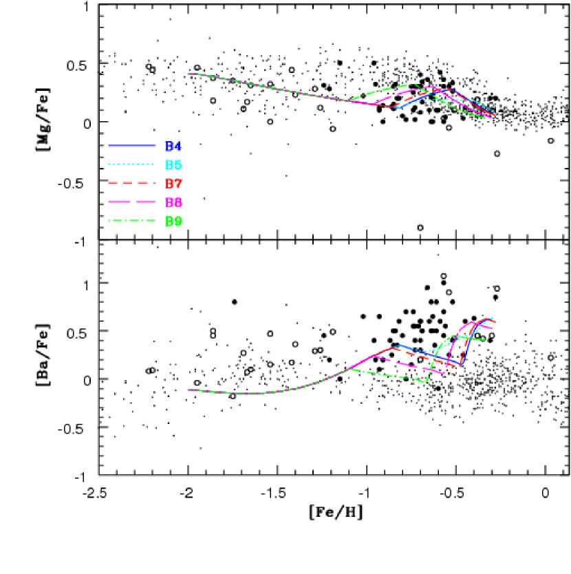
Figure 20: Chemical evolution on the [Mg/Fe]-[Fe/H] plane (upper) and the [Ba/Fe]-[Fe/H] one (lower) for the five starburst models with different epoch and duration of starburst; B4 (blue solid), B5 (cyan dotted), B7 (red short-dashed), B8 (magenta long-dashed), and B9 (green dot-dashed).

However, as pointed out in previous sections, these three chemical signatures of the past starburst event around 2 Gyr ago can not be clearly seen in the observational results. Figure 20 shows [Mg/Fe]–[Fe/H] and [Ba/Fe]–[Fe/H] relations for the five burst models (B4$-$B9) with different epochs and strengths of starburst. The results shown in this figure (and Figure 8) suggest that although the observed higher [Mg/Fe] ($>0.2$) at [Fe/H]$\sim-0.6$ can be consistent with the rapid increase of [Mg/Fe] due to the starburst event, the large scatter in [Mg/Fe] around [Fe/H]$\sim-0.6$ does not allow us to make a robust conclusion on the origin of the higher [Mg/Fe]. Similarly, the observed larger [Ba/Fe] ($>0.5$) for [Fe/H]$>-0.4$, which is consistent with the present starburst models, can not be regarded as strong evidence for the presence of a starburst about 2 Gyr ago owing to the small number of stars with known [Ba/Fe] for [Fe/H] $>-0.4$. More observational data sets are necessary to investigate how the secondary starburst about 2 Gyr ago might have changed the chemical evolution history of the LMC. The AMRs derived by different observational studies are significantly different so that the comparison between the observed AMRs and the simulated ones in the present study can not provide strong constraints on the nature of the past starburst events either.

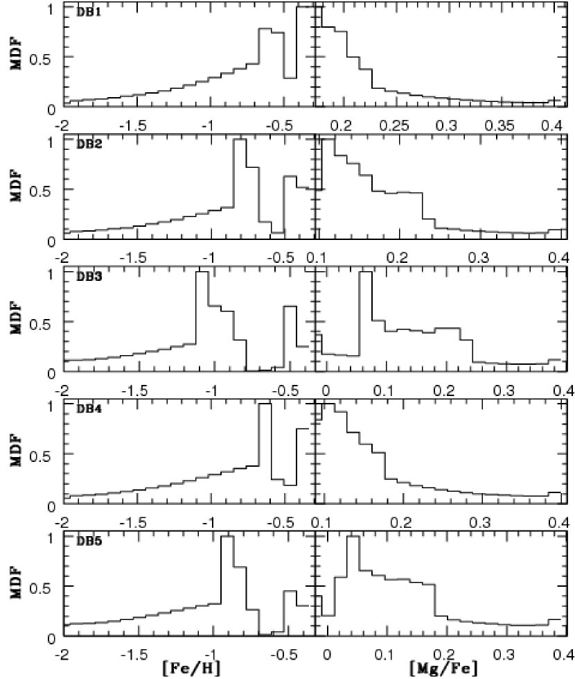
Figure 21: The MDFs for [Fe/H] (left) and [Mg/Fe] (right) in the five double-burst models, DB1 (top), DB2 (second from the top), DB3 (middle), DB4 (second from the bottom), and DB5 (bottom). The MDFs are normalized to the maximum numbers of stars in the bins.

Concerning a possible starburst about 0.2 Gyr ago, a chemical signature of the starburst about 0.2 Gyr ago is the sudden increase of [Mg/Fe] around [Fe/H]$\sim-0.4$, as shown in the present double-burst models. There is a hint of such a [Mg/Fe] increase in the observational data for the LMC field stars by P08, though the number of the stars is very small (only three). If the starburst is strong enough, then it can be imprinted on the MDF of the LMC. Figure 21 describes the MDFs for [Fe/H] and [Mg/Fe] in the five double-burst models. The MDFs here are relative frequency histograms that are binned with 0.1 dex bin width and normalized to the most populated bin. Clearly the MDF of [Fe/H] show the double peaks for the five models and such double peaks are not observed in the previous observation by C08. The observed apparent lack of a bimodal MDF in C08 could be due to the small number of young and metal-rich samples in C08. If the observational result is real, then it means that the starburst about 0.2 Gyr ago is much weaker than modeled in the present study (so that it can not be detected in the observed MDF).

4.4 The origin of the dip in the AMR

The AMR derived for the LMC by HZ09 (in their Figure 20) appears to show a sudden and significant decrease of [Fe/H] around 1.5 Gyr ago followed by a rapid increase of [Fe/H], though HZ09 did not discuss the origin of the possible “dip” in the AMR. The AMRs for some local regions of the LMC derived by R12 also appear to show the dips whereas the AMR by C08 does not clearly show the dip. If the observed dip around 1.5 Gyr ago (HZ09) is real, it has profound implications on the gas accretion history of the LMC. One of likely explanations for the possible dip is that a large amount of external metal-poor gas ([Fe/H] $<-1.0$, significantly smaller than the gaseous metallicity of the LMC about 2 Gyr ago) was accreted onto the LMC from outside the LMC disk and consequently [Fe/H] rapidly and significantly decreased. The observed apparently rapid decrease of [Fe/H] by almost 0.2 dex at [Fe/H]$\sim-0.7$ (HZ09) can give some constraints on the amount of gas accreted onto the LMC for a given metallicity of the metal-poor gas.

In order to discuss how the AMR of the LMC can change owing to the infall of metal-poor gas from outside the LMC disk, we have investigated the AMRs of models with gas infall yet without any starburst before infall. The purpose of this investigation is to show clearly how the dip of the AMR can be formed during the infall of metal-poor gas (thus not to reproduce the observed AMR fully self-consistently). Therefore, we think that the adopted somewhat idealized models would be enough to show clearly the formation of the dip in the AMR due to the infall of metal-poor gas. We have mainly investigated how much gas needs to be accreted onto the LMC by using the results of the “infall models” in which metal-poor gas with [Fe/H]=$-1.6$ can be accreted onto the LMC at 1.5 Gyr ago. Here the metallicity of [Fe/H]$=-1.6$ is chosen just for a representative case to clearly show the formation of the dip in the AMR (we also investigated the infall models with [Fe/H]$=-1.0$ for comparison).

In the infall models, the following infall rate of external gas ($\dot{M}_{\rm ext}$) is added to the right side of the equation (1):

$$\dot{M}_{\rm ext}=\frac{M_{\rm ext}}{t_{\rm in,e}-t_{\rm in,s}},$$ (12)

where $M_{\rm ext}$ is the total mass of the external gas that can infall onto the LMC for $t_{\rm in,s}\leq t\leq t_{\rm in,e}$, where $t_{\rm in,s}$ and $t_{\rm in,e}$ are the epochs when the gas infall starts and ends, respectively. Therefore, the gas infall rate is assumed to be steady and constant in the present infall models. We investigate the models with $t_{\rm in,s}=11.5$ Gyr and $t_{\rm in,e}=12.0$ Gyr. The chemical abundance patterns of the gas is assumed to be the same as that of the LMC halo. Therefore, the term of $Z_{I,i}\dot{M}_{\rm ext}$ (where $Z_{I,i}$ is the chemical abundance of each element in the infalling gas) is added to the right hand side of equation (2) to calculate the evolution of $Z_{i}$. Owing to the infall of metal-poor gas, the mean metallicity of the youngest population becomes significantly lower. Therefore, a starburst needs to occur after the gas infall so that the final [Fe/H] can be $-0.3$, as observed. We thus assume that starbursts can occur before and after accretion of the metal-poor gas onto the LMC disk in the infall models, because the models with this assumption can be consistent also with the observational results by HZ09 (i.e., a possible starburst about 2 Gyr ago). We have particularly investigated the four infall models (I1$-$I4) with $\alpha=2.55$ and $C_{\rm q}=0.004$, $C_{\rm sb1}=0.8$, $t_{\rm sb1,s}=11.0$ Gyr, $t_{\rm sb1,e}=11.1$ Gyr, $t_{\rm sb2,s}=12.0$, $t_{\rm sb2,e}=13.0$ Gyr, [Fe/H]$=-1.6$ in external infalling gas, and different $C_{\rm sb2}$ and $M_{\rm ext}$. These models were chosen because they can together show different degrees of sudden [Fe/H] drop (or different depths of the dip) in the AMRs. For comparison, we have investigated a model (I5) with [Fe/H]$=-1.0$ in external gas for comparison. The model parameters for these models are shown in Table 4.

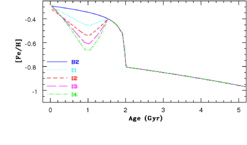
Figure 22: The AMRs for the last $\sim 5$ Gyr for the burst model B2 (blue solid) and the four infall models, I1 with $M_{\rm ext}=0.1$ (cyan dotted), I2 with $M_{\rm ext}=0.2$ (red short-dashed), I3 with $M_{\rm ext}=0.3$ (magenta long-dashed), and I4 with $M_{\rm ext}=0.4$ (green dot-dashed). Here $M_{\rm ext}$ represents the total mass of external metal-poor gas accreted onto the LMC. $M_{\rm ext}=1$ thus means that the total amount of external gas accretion is the same as the total amount of gas accreted onto the LMC from its own halo for the last 13 Gyr. Infall of external metal-poor gas onto the LMC disk is assumed to commence 1.5 Gyr ago and end 1 Gyr ago in these four infall models. Starbursts are assumed to occur twice at 2 Gyr ago and 1 Gyr (just after the end of the external gas infall event) in these infall models so that the final stellar metallicity in each model can be the same as the observed one ([Fe/H]$\sim-0.3$).

Figure 22 shows the AMRs for the last $\sim 5$ Gyr (i.e., $t=8-13$ Gyr) in the four infall models in which $M_{\rm ext}$ ranges from 0.1 to 0.4 in simulation units. $M_{\rm ext}=1$ thus means that the total amount of external gas accretion is the same as the total amount of gas accreted onto the LMC from its own halo for the last 13 Gyr. The value of $C_{\rm sb2}$ in each model is chosen such that the final [Fe/H] can be consistent with the observed one. For comparison, the AMR of the burst model B2 without gas infall is shown in this figure. Clearly stellar [Fe/H] can rapidly decrease soon after the metal-poor gas is accreted onto the LMC with the magnitude of the decrease depending on the amount of the accreted gas ($M_{\rm ext}$). The model I3 with $M_{\rm ext}=0.3$ can show the dip of $\sim 0.2$ dex, which means that $\sim 10^{9}M_{\odot}$ needs to be accreted onto the LMC for explaining the observed dip. Other models with lower $M_{\rm ext}$ (i.e., I1 and I2) show less remarkable dips in the AMRs and thus are less consistent with the observations. If the metallicity of the accreted gas is higher than the adopted one ([Fe/H]=$-1.6$), then even a larger amount of gas needs to be accreted onto the LMC to form the remarkable dip in the AMR. For example, if the infalling gas has [Fe/H]$=-1$, then $M_{\rm ext}\approx 0.4$ is required for explaining the dip of $\sim 0.2$ dex observed in the AMR. We thus conclude that if the observed dip is real, then a massive accretion event of metal-poor gas with $M_{\rm ext}$ of at least $\sim 10^{9}M_{\odot}$ is required to explain the observed magnitude of the dip.

Previous numerical simulations by BC07 and DB12 demonstrated that the gas of the SMC can be accreted onto the LMC after tidal stripping of the SMC gas caused by the strong LMC–SMC–Galaxy interaction. These simulations showed that there could be two accretion events around 1.5 Gyr and 0.2 Gyr ago, which means that the first accretion event about 1.5 Gyr ago is a promising candidate which can provide a large enough amount of gas to form the dip in the LMC AMR. However, the total amount of the SMC gas transferred to the LMC about 1.5 Gyr ago in these simulations is less than $10^{8}{\rm M}_{\odot}$ for the total SMC mass of $3\times 10^{9}M_{\odot}$. The predicted gas mass is much smaller than the required mass ($M_{\rm ext}\sim 10^{9}M_{\odot}$) for explaining the observed dip. This means that the SMC gas accreted onto the LMC is unlikely to explain the observed dip of 0.2 dex, if the total mass of the SMC about 2 Gyr ago is similar to that of the present SMC ($\sim 3\times 10^{9}M_{\odot}$). However, if the SMC was originally much more massive, the required amount of gas mass could be transferred from the SMC to the LMC.

Then where does such a large amount of metal-poor gas come from? One possible scenario is that a gas-rich dwarf galaxy with a total gas mass of $10^{9}M_{\odot}$ merged with the LMC about 1.5 Gyr ago and the mixing of the gas with the LMC ISM caused a significant decrease of [Fe/H]. Since the gas-mass of the dwarf should be similar to that of the LMC in order to explain the observed dip, the dwarf would have to have had a total mass similar to the LMC. This means that the LMC stellar disk could have been severely damaged by the violent dynamical process of such a major merger event. The thick disk and counter-rotating stellar components (e.g., Subramaniam & Prabhu 2005) might have been formed from this major merger event occurring in the LMC about 1.5 Gyr ago. A merged dwarf as massive as the LMC should have a much lower star formation rate than the LMC so that it can have a low metallicity. This discussion depends on the assumption that the observed dip of 0.2 dex is real and the dip was caused by a massive gas accretion event. Given that the amplitude of the dip provides information about the total mass of a gas-rich dwarf merging with the LMC (or the total mass of gas accretion onto the LMC), it would be quite important for future extensive observational studies to confirm the presence or the absence of the dip(s) in the AMR.

4.5 Formation of very high [Ba/Fe] stars in the LMC

Although the present models can reproduce reasonably well the overall trend of [Ba/Fe] with [Fe/H] and the higher [Ba/Fe] ($\sim 0.5$) for [Fe/H]$<-0.6$ in the LMC, they can not explain the stars with [Ba/Fe]$>0.9$. We have confirmed that even the selective wind models with steep IMFs and efficient metal ejection ($f_{\rm ej}\sim 0.6$) can show at most [Ba/Fe]$\sim 0.8$. This failure of the present one-zone chemical evolution models is related to the adopted assumption that AGB ejecta can be mixed with ISM soon after AGB stars eject their $s$-process elements. If the AGB ejecta does not mix well with the surrounding ISM and consequently can be converted into new stars, then the stars can show rather high [Ba/Fe]: Figure 1 in TB12 shows the observed rather high ($>1$) [Ba/Fe] in the envelope of AGB stars with different metallicities. We thus propose that the stars with unusually high [Ba/Fe] ($>0.9$) in the LMC were formed as a result of incomplete mixing of ISM and AGB ejecta. A key question here is how energetic stellar winds from AGB stars can cool down to become cold gas for star formation without mixing so well with the surrounding ISM.

Recent hydrodynamical simulations have shown that secondary star formation directly from AGB ejecta is possible in massive star clusters owing to the deeper gravitational potentials (e.g., Bekki 2011). Although this secondary star formation appears to be a convincing mechanism for the formation of stars with unusually high [Ba/Fe] in the LMC GCs, it can not explain why some of the LMC field stars show such high [Ba/Fe]. One possibility for the field star formation from AGB ejecta is that AGB ejecta can assemble in the HI holes (e.g., Kim et al. 1999), where ISM can be almost completely blown away by SNe, and then can be converted into cold gas there without mixing efficiently with chemically enriched ISM. The new stars formed from AGB ejecta in the HI holes can naturally have very high [Ba/Fe]. Thus it would be important for observational studies to confirm whether the locations of young stars with very high [Ba/Fe] are more likely to be in the present HI holes. Our future chemodynamical simulations will investigate whether this star formation from AGB ejecta in HI holes is really possible in the LMC.

5 Conclusions

We have investigated the chemical evolution of the LMC by using new one-zone chemical evolution models in which both chemical pollution by prompt SNe Ia and metallicity dependent chemical yields of AGB stars are incorporated and the IMF is a free parameter. We have particularly investigated three different types of models with or without starburst (i.e., standard, burst, and double-burst models) so that we can discuss the importance of previous starbursts in the history of the chemical evolution of the LMC. We furthermore have investigated the wind models in which gaseous ejecta from AGB stars, SNe Ia, and SNe II can be removed partly from the LMC owing to stellar feedback effects of SNe and AGB stars. The principle results of the models are summarized as follows.

(1) The observed gas mass fraction ($f_{\rm g,0}\sim 0.3$) and the metallicity of youngest stellar populations ([Fe/H]${}_{0}\sim-0.3$) in the LMC together give some constraints on the IMF and the efficiency of gas removal by stellar feedback effects. Both $f_{\rm g}$ and [Fe/H]₀ can be best reproduced by a steeper IMF with $\alpha=2.55$ for the standard (i.e., no burst) models in a self-consistent manner, if the gaseous ejecta from AGB stars and SNe are not removed from the LMC (i.e., non-wind models). This tendency of steeper IMFs to better explain $f_{\rm g}$ and [Fe/H]₀ simultaneously can be seen also in the burst and double-burst models. Furthermore, the observed higher [Ba/Fe] ($>-0.2$) of stars in GCs at [Fe/H]$<-1.5$ in the LMC is also more consistent with steeper IMFs ($\alpha>2.55$).

(2) However, the models with the Salpeter IMF ($\alpha=2.35$) can also explain the observed $f_{\rm g,0}$ and [Fe/H]₀, if significant fractions ($f_{\rm ej}\sim 0.4$) of gaseous ejecta from SNe are selectively removed from the LMC (i.e., no removal of AGB ejecta). These selective wind models are significantly more reasonable than the uniform wind ones proposed by PT98 in which ISM, AGB ejecta, and supernova ones are equally removed. This is because an unreasonably large amount of gas ($\sim 10^{10}M_{\odot}$, or three times the present stellar mass of the LMC) need to be removed from the LMC for the best uniform wind models with the Salpeter IMF. The wind models with the Salpeter IMF, however, can not reproduce well the observed higher [Ba/Fe] ($>-0.2$) at lower [Fe/H] ($<-1.5$). Thus, although removal of SNe ejecta could be important in the chemical evolution of the LMC, an IMF steeper than the Salpeter one is required for explaining $f_{\rm g,0}$, [Fe/H]₀, and [Ba/Fe] at low [Fe/H] in a self-consistent manner.

(3) The present models predict that [$\alpha$/Fe] starts to decrease monotonically only $\sim 10^{8}$ yr after the commencement of active star formation in the LMC owing to rapid chemical enrichment by ejecta from prompt SNe Ia. The observed [Ca/Fe]–[Fe/H] relation with the apparent lack of the plateau can be consistent with models with chemical pollution by prompt SNe Ia rather than by classical ones. This suggests that the observed [Ca/Fe]–[Fe/H] relation is supporting evidence for prompt SNe Ia playing a key role in the chemical evolution of the LMC. However, it should be noted that [Mg/Fe] does not so show such a clear trend as decreasing [Mg/Fe] with increasing [Fe/H] (like [Ca/Fe]–[Fe/H] relation) for the entire sample of stars and GCs.

(4) The present models predict that if the LMC experienced a starburst about 2 Gyr ago, [$\alpha$/Fe] can start to rapidly increase (up to 0.3) at [Fe/H]$\sim-0.5$ owing to gaseous ejecta of SNe II and then soon decrease owing to the Fe-rich ejecta from prompt SNe Ia. Therefore, the best model predicts a “bump” in the [$\alpha$/Fe]–[Fe/H] relation around [Fe/H]$\sim-0.5$, though such a bump can not be so clearly seen in the observed [$\alpha$/Fe]–[Fe/H] relation owing to the apparently large scatter of [$\alpha$/Fe] at [Fe/H]$\sim-0.5$. The observed presence of stars with [Mg/Fe]$>0.3$ at $-0.6<$[Fe/H]$<-0.5$ and the observed apparent lack of stars with [Mg/Fe]$<0.2$ at $-0.5<$[Fe/H]$<-0.3$ can be consistent with the presence of the bump, though the smaller number of observational data points for [Fe/H]$>-0.5$ could be responsible for the apparent dip.

(5) If the LMC experiences a secondary starburst, [Ba/Fe] temporarily decreases owing to Fe-rich ejecta from SNe II and prompt SNe Ia then increases sharply owing to AGB ejecta that is rich in $s$-process elements. For example, if the LMC experienced a starburst about 2 Gyr ago when the LMC had [Fe/H]$\sim-0.7$, then the LMC shows the [Ba/Fe] peak at [Fe/H]$\sim-0.3$ in the [Ba/Fe]–[Fe/H] relation. Furthermore, [Ba/Fe] can show its peak (up to $\sim 0.7$) always after [$\alpha$/Fe] takes its peak value. As a natural result of this, [Fe/H] at the [Ba/Fe] peak is higher than that at the [$\alpha$/Fe] peak in the [Ba/Fe]–[Fe/H] and [$\alpha$/Fe]–[Fe/H] relations. These predicted trends of [Ba/Fe] are not so clearly seen in the observed [Ba/Fe]–[Fe/H] relation owing to the large scatter of [Ba/Fe]. However, the observed larger [Ba/Fe] at [Fe/H] $\sim-0.3$ is more consistent with the present burst models (in particular with those of steeper IMFs). However, the observed very large [Ba/Fe] $\sim 1$ at [Fe/H]$\sim-0.5$ in some field stars and GCs of the LMC can not be simply explained by any model in the present study. Thus we have proposed that such very high [Ba/Fe] stars could be formed from AGB ejecta that did not mix well with ISM.

(6) The observed AMR has a large scatter, so the standard (non-burst), burst, and double-burst models can be all consistent with the AMR, which implies that the AMR does not give strong constraints on the LMC star formation history. The present double-burst models have bimodal distributions of [Fe/H] (i.e., two peaks in the MDF), which have not been observed yet. Therefore, the double-burst models are the least consistent with observations among the three different types of models investigated in the present study in terms of the MDF. Accordingly, we suggest that the observationally inferred recent starburst around 0.1–0.5 Gyr ago by HZ09 should be weak so as to reproduce the observed MDF.

(7) If the observed apparent dip (i.e., a sudden [Fe/H] decrease by $\sim 0.2$ dex) in the AMR around 1.5 Gyr ago is real, then it has a profound implication for the gas accretion history of the LMC. The present models predict that the dip could be due to the accretion of a large amount ($\sim 10^{9}M_{\odot}$) of metal-poor gas ([Fe/H]$<-1$) from other gas-rich galaxies about 1.5 Gyr ago. Given that previous numerical simulations (e.g., BC07 and DB12) demonstrated a gas transfer from the SMC to the LMC caused by tidal stripping of the SMC about 1.5 Gyr ago, the SMC gas could be responsible for the gas accretion event in the LMC. However, the required large amount of gas ($\sim 10^{9}M_{\odot}$) is much larger than the predicted amount ($\sim 10^{8}M_{\odot}$) in previous simulations. There can be two possible scenarios for the gas transfer. One is that the SMC was originally much more massive than the present SMC, as suggested by the recent modeling of the SMC’s rotation curve (Bekki & Stanivirovic 2009), so that a large amount of gas can be transferred from the SMC to the LMC. The other is that the LMC experienced a major merger with a massive gas-rich dwarf galaxy. Such a gas-rich major merger event may be responsible for the formation of the thicker and extended stellar disk observed in the LMC.

(8) The observed rather low [Ca/Fe] ($<-0.2$) at [Fe/H]$>-0.6$ in the LMC field stars can not be simply explained by the present models, in which all elements of SNe are equally efficiently removed from the LMC. We have thus proposed that if Ca can be (by a factor of $\sim 2$) more efficiently removed from the LMC through supernova feedback effects in comparison with other elements, then the observed unusually low [Ca/Fe] and normal [Mg/Fe] for [Fe/H]$>-0.6$ can be simultaneously explained. Although it remain unclear why such more efficient removal of Ca should occur in the chemical enrichment history of the LMC, we have proposed that a characteristic nucleosynthesis of jet-induced SNe can be associated with the origin of the field stars with unusually low [Ca/Fe]. The origin of the higher [Ca/Fe] in the intermediate-age GCs of the LMC remains unclear.

(9) The differences in IMFs and removal efficiencies of AGB and SN ejecta between the LMC and the Galaxy might be responsible for the observed clear differences in the locations of the stars in the [$\alpha$/Fe]–[Fe/H] and [Ba/Fe]–[Fe/H] relations between the two galaxies. Our future chemodynamical simulations of the star formation and chemical enrichment histories in the LMC will investigate how and why the IMF and the removal processes of stellar ejecta of the two galaxies might be different. We plan to discuss the spatially different chemical properties in the LMC based on the results of the simulations.

Table 1: Model parameters for one-zone chemical evolution

Model	$\alpha$	$C_{\rm q}$	$C_{\rm sb1}$	$t_{\rm sb1,s}$	$t_{\rm sb1,e}$	$C_{\rm sb2}$	$t_{\rm sb2,s}$	$t_{\rm sb2,e}$	$f_{\rm ej}$	$C_{\rm ej}$
S1	2.35	0.006	-	-	-	-	-	-	-	-
S2	2.15	0.004	-	-	-	-	-	-	-	-
S3	2.55	0.01	-	-	-	-	-	-	-	-
S4	2.75	0.017	-	-	-	-	-	-	-	-
S5	2.95	0.02	-	-	-	-	-	-	-	-
B1	2.35	0.004	0.3	11.0	11.1	-	-	-	-	-
B2	2.55	0.004	0.8	11.0	11.1	-	-	-	-	-
B3	2.75	0.004	1.2	11.0	11.1	-	-	-	-	-
B4	2.55	0.006	0.5	11.0	11.1	-	-	-	-	-
B5	2.75	0.006	1.4	11.0	11.1	-	-	-	-	-
B6	2.35	0.004	0.03	11.0	12.0	-	-	-	-	-
B7	2.55	0.004	0.8	10.0	10.1	-	-	-	-	-
B8	2.55	0.004	0.8	8.0	8.1	-	-	-	-	-
B9	2.35	0.004	0.6	6.0	6.1	-	-	-	-	-
DB1	2.35	0.004	0.2	11.0	11.1	0.2	12.8	12.9	-	-
DB2	2.55	0.004	0.55	11.0	11.1	0.55	12.8	12.9	-	-
DB3	2.75	0.004	1.0	11.0	11.1	1.0	12.8	12.9	-	-
DB4	2.55	0.006	0.4	11.0	11.1	0.4	12.8	12.9	-	-
DB5	2.75	0.006	0.9	11.0	11.1	0.9	12.8	12.9	-	-
DB6	2.35	0.004	0.15	11.0	11.1	0.15	12.5	12.6	-	-
W1	2.35	0.01	-	-	-	-	-	-	0.4	-
W2	2.55	0.015	-	-	-	-	-	-	0.4	-
W3	2.35	0.008	-	-	-	-	-	-	0.2	-
W4	2.55	0.012	-	-	-	-	-	-	0.2	-
W5	2.35	0.012	-	-	-	-	-	-	0.2	300.0
W6	2.55	0.015	-	-	-	-	-	-	0.4	-

ⁱ The time at which the second starburst ends in units of Gyr.
^j The mass fraction of SN ejecta that can be completely removed from the LMC in the selective wind models.
^k The coefficient for the metal ejection rate in the non-selective wind models.

Table 2: Comparison of different models

Properties/models	Standard	Burst	Double-burst	Wind
AMR	$\bigcirc$	$\bigcirc$	$\bigcirc$	$\bigcirc$
${\rm[Mg/Fe]-[Fe/H]}$	$\bigcirc$	$\bigcirc$	$\bigcirc$	$\bigcirc$
a bump in the ${\rm[Mg/Fe]-[Fe/H]}$ relation	$\times$	$\bigcirc$	$\bigcirc$	$\bigcirc$
${\rm[Mg/Fe]}$ at ${\rm[Fe/H]_{0}}$	$\bigcirc$	$\bigcirc$	$\bigcirc$	$\bigcirc$
${\rm[Ba/Fe]-[Fe/H]}$	$\bigcirc$	$\bigcirc$	$\bigcirc$	$\bigcirc$
high ($\sim 0.5$) ${\rm[Ba/Fe]}$ at ${\rm[Fe/H]}\sim-0.3$	$\bigcirc$	$\bigcirc$	$\bigcirc$	$\bigcirc$
very high ($>0.9$) ${\rm[Ba/Fe]}$ at ${\rm[Fe/H]}\sim-0.6$	$\times$	$\times$	$\times$	$\times$
${\rm[Ba/Fe]}$($>-0.2$) of GCs at ${\rm[Fe/H]}<-1.5$	$\bigcirc$	$\bigcirc$	$\bigcirc$	$\bigcirc$
$f_{\rm g,0}-{\rm[Fe/H]}_{0}$	$\bigcirc$	$\bigcirc$	$\bigcirc$	$\bigcirc$

Table 3: Constraints on the IMF and the star formation history in the LMC

Properties	Requirement
a bump in the ${\rm[Mg/Fe]-[Fe/H]}$ relation	starburst about 2 Gyr ago
high ($\sim 0.5$) ${\rm[Ba/Fe]}$ at ${\rm[Fe/H]}\sim-0.3$	$\alpha\geq 2.55$ in non-wind models
${\rm[Ba/Fe]}$($>-0.2$) of GCs at ${\rm[Fe/H]}<-1.5$	$\alpha\geq 2.55$
$f_{\rm g,0}-{\rm[Fe/H]}_{0}$	$\alpha\sim 2.55$ in non-wind models

Table 4: Parameters for the infall models

Model	$M_{\rm ext}$	[Fe/H] in external gas	$C_{\rm sb2}$
I1	0.1	-1.6	0.05
I2	0.2	-1.6	0.07
I3	0.3	-1.6	0.1
I4	0.4	-1.6	0.12
I5	0.4	-1.0	0.12

References

- (1) Ardeberg, A., Gustafsson, B., Linde, P., & Nissen, P.-E. 1997, A&A, 322, L13
- (2) Bekki, K. 2011, MNRAS, 412, 2241
- (3) Bekki, K., & Chiba, M. 2005, MNRAS, 356, 680
- Bekki & Chiba (2007) Bekki, K., & Chiba, M. 2007, MNRAS, 381, L16 (BC07)
- (5) Bekki, K. Campbell, S. W. Lattanzio, J. C., & Norris, J. E. 2007, MNRAS, 377, 335
- (6) Bekki, K., & Sanimirovic, S. 2009, MNRAS, 395, 342
- (7) Bekki, K., & Tsujimoto, T., 2010, ApJ, 721, 1515
- (8) Bell, E. F., & de Jong, R. S. 2001, ApJ, 550, 212
- Bensby et al. (2005) Bensby, T., Feltzing, S., Lundström, I., & Ilyin, I. 2005, A&A, 433, 185
- (10) Bernard, J.-P., et al. 2008, AJ, 136 919
- (11) Bertelli, G., Mateo, M. Chiosi, C., & Bressan, A. 1992, ApJ, 388, 400
- (12) Bica, E., Dottori, H., & Pastoriza, M. 1986, A&A, 156, 261
- Busso et al. (2001) Busso, M., Gallino, R., Lambert, D. L., Travaglio, C., & Smith, V. V. 2001, ApJ, 557, 802
- (14) Butcher, H. 1977, ApJ, 216, 372
- (15) Carrera, R., Gallart, C., Hardy, E., Aparicio, A., & Zinn, R. 2008, AJ, 135, 836 (C08)
- (16) Cioni, M.-R. L., Girardi, L., Marigo, P., & Habing, H. J. 2006, A&A, 448, 77
- Colucci et al. (2012) Colucci, J. E., Bernstein, R. A., Cameron, S. A., & McWilliam, A. 2012, ApJ, 746, 29 (C12)
- (18) Cole, A. A., Tolstoy, E., Gallagher, J. S. III., & Smecker-Hane, T. A. 2005, AJ, 129, 1465 (C05)
- (19) Da Costa G. S. 1991, in Haynes R., Milne D., eds, Proc. IAU Symp. 148, The Magellanic Clouds, Kluwer, Dordrecht, p183
- Diaz & Bekki (2012) Diaz, J. D., & Bekki, K. 2012, ApJ, in press, arXiv1112.6191, (DB12)
- (21) Dopita, M. A., et al. 1997, ApJ, 474, 188
- (22) Elson R. A. W., Gilmore, G. F., & Santiago, B. X. 1997, MNRAS, 289, 157
- (23) Gallagher et al. 1996, ApJ, 466, 732
- Gallino et al. (1998) Gallino, R., et al. 1998, ApJ, 497, 388
- (25) Geha, M. C., et al. 1998, AJ, 115, 1045
- (26) Geisler, D., Bica, E., Dottori, H., Claria, J. J., Piatti, A. E., & Santos, J. F. C., Jr. 1997, AJ, 114, 1920
- (27) Geisler, D., Piatti, A. E., Bica, E., Clariá, J. J. 2005, MNRAS, 341, 771
- (28) Glatt, K., Grebel, E. K., & Koch, A. 2010, A&A, 517, 50
- Gratton et al. (2003) Gratton, R. G., Carretta, E., Claudi, R., Lucatello, S., & Barbieri, M. 2003, A&A, 404, 187
- (30) Harris J., & Zaritsky D., 2009, AJ, 138, 1243 (HZ09)
- (31) Hascheke, R., et al. 2012 in preprint (arXiv:1207.5791)
- (32) Hill, V., Andrievsky, S., & Spite, M. 1995, A&, 293, 347
- (33) Hill, V., Frano̧is, P., Spite, M., Primas, F., & Spite, F. 2000, A&A, 364, L19
- (34) Holtzman, J. A., et al. 1997, AJ, 113, 656
- (35) Holtzman et al. 1998, AJ, 115, 1946
- (36) Indu, G., & Subramaniam, A. 2011, A&A, 535, 115
- (37) Hill, R. J., Madore, B. F., & Freedman, W. L. 1994, ApJ, 429, 204
- Ishimaru & Wanajo (1999) Ishimaru, Y., & Wanajo, S. 1999, ApJ, 511, L33
- Johnson et al. (2006) Johnson, J. A., Ivans, I. I., & Stetson, P. B. 2006, ApJ, 640, 801
- Kim et al. (1999) Kim, S., Dopita, M. A., Staveley-Smith, L., & Bessel, M. 1999, AJ, 118, 2823
- (41) Luck, R. E., Moffett, T. J., Barnes, T. G. III., & Gieren, W. P. 1998, AJ, 115, 605
- Mannucci et al. (2006) Mannucci, F., Della Valle, M., & Panagia, N. 2006, MNRAS, 370, 773
- Maoz et al. (2010) Maoz, D., Sharon, K., & Gal-Yam, A. 2010, ApJ, 722, 1879
- (44) Maoz, D., Mannucci, F., Li, W., Filippenko, A. V., Della Valle, M., & Panagia, N. 2011, MNRAS, 412, 1508
- (45) Maoz, D., & Badenes, C. 2010, MNRAS, 407, 1314
- (46) Mateo, M. 1988, ApJ, 331, 261
- Mathews et al. (1992) Mathews, G. J., Bazan, G., & Cowan, J. J. 1992, ApJ, 391, 719
- Mucciarelli et al. (2008) Mucciarelli, A., Carretta, E., Origlia, L., & Ferraro, F. R. 2008, AJ, 136, 375
- Mucciarelli et al. (2010) Mucciarelli, A., Origlia, L., & Ferraro, F. R. 2010, ApJ, 717, 277 (M10)
- Mucciarelli et al. (2011) Mucciarelli, A., et al. 2011, MNRAS, 413, 837 (M11)
- (51) Olszewski, E. W., Schommer, R. A., Suntzeff, N. B., & Harris, H. C. 1991, AJ, 101, 515
- (52) Olsen, K. A. G. 1999, AJ, 117, 2244
- (53) Olsen, K. A. G., Zaritsky, D., Blum, R. D., Boyer, M. L., & Gordon, K. D. 2011, ApJ, 737, 29
- (54) Olszewski, E. W., Suntzeff, N. B. & Mateo, M. 1996, ARA&A, 34, 511
- (55) Piatti, A. E. 2011, MNRAS, 418, L40
- Pagel & Tautvaišiené (1998) Pagel, B. E. J., & Tautvaišiené, G. 1998, MNRAS, 299, 535 (PT98)
- (57) Pilyugin, L. S. 1996, A&A, 313, 803
- Pompéia et al. (2008) Pompéia, L., et al. 2008, A&A, 480, 379 (P08)
- Reddy et al. (2003) Reddy, B. E., Tomkin, J., Lambert, D. L., & Allende Prieto, C. 2003, MNRAS, 340, 304
- (60) Renzini, A., & Buzzoni, A., 1986, in Spectral Evolution of Galaxies, Reidel, Dordrecht, p.195
- (61) Rubele, S., et al., 2012, A&A, 537, 106
- (62) Russell, S. C., & Dopita, M. A. 1992, ApJ, 384, 508
- (63) Salpeter, E. E. 1955, ApJ, 121, 161
- (64) Shigeyama, T., et al. 2010, AIPC, 1279, 415
- (65) Smecker-Hane, T. A., Cole, A. A., Gallagher, J. S. III, & Stetson, P. B. 2002, ApJ, 566, 239.
- (66) Stryker, L. 1983, ApJ, 266, 82
- (67) Subramaniam, A., & Prabhu, T. P. 2005, ApJ, L47
- Totani et al. (2008) Totani, T., Morokuma, T., Oda, T., Doi, M., & Yasuda, N. 2008, PASJ, 60, 1327
- Tsujimoto (2012) Tsujimoto, T. 2012, ApJ, 736, 113
- (70) Tsujimoto, T., Nomoto, K., Yoshii, Y., Hashimoto, M., Yanagida, S., & Thielemann, F.-K. 1995, MNRAS, 277, 945 (T95)
- (71) Tsujimoto, T., Bland-Hawthorn, J., & Freeman, K. C. 2010, PASJ, 62, 447
- (72) Tsujimoto, T., & Bekki, K. 2012, ApJ, 747, 125 (TB12)
- (73) Vallenari, A., Chiosi, C., Bertelli, G., Aparicio, A., & Ortolani, S. 1996, A&A, 309, 367
- (74) Weidemann, V. 2000, A&A, 363, 647
- Wheeler et al. (1998) Wheeler, J. C., Cowan, J. J., & Hillebrandt, W. 1998, ApJ, 493, 101
- Yoshii et al. (1996) Yoshii, Y., Tsujimoto, T., & Nomoto, K. 1996, ApJ, 462, 266