Abstract

It has been established that the entangled polymer dynamics can be reasonably described by single chain models such as tube and slip-link models. Although the entanglement effect is a result of the hard-core interaction between chains, linkage between the single chain models and the real multi-chain system has not been established yet. In this study, we propose a multi-chain slip-spring model where bead-spring chains are dispersed in space and connected by slip-springs inspired by the single chain slip-spring model [A. E. Likhtman, Macromolecules 38, 6128 (2005)]. In this model the entanglement effect is replaced by the slip-springs, not by the hard-core interaction between beads so that this model is located in the niche between conventional multi-chain simulations and single chain models. The set of state variables are the position of beads and the connectivity (indices) of the slip-springs between beads. The dynamics of the system is described by the time evolution equation and stochastic transition dynamics for these variables. We propose a simple model which is based on the well-defined total free-energy and the detailed balance condition. The free energy in our model contains a repulsive interaction between beads, which compensate the attractive interaction artificially generated by the slip-springs. The explicit expression of linear relaxation modulus is also derived by the linear response theory. We also propose a possible numerical scheme to perform simulations. Simulations reproduced expected bead number dependence in transitional regime between Rouse and entangled dynamics for the chain structure, the central bead diffusion, and the linear relaxation modulus.
KEY WORDS:
Entangled polymers; Brownian simulations; 3D multi-chain network; Free energy;

1 Introduction

It has been rather established that the entangled polymer dynamics can be reasonably described by single chain models where the effect of entanglement is replaced by dynamical constraints such as tubes or slip-links[1, 2, 3, 4]. For instance, several single chain models[5, 6, 7, 8, 9, 10, 11] have been proposed to reproduce viscoelasticity, diffusion, dielectric relaxation, etc, by taking account the relevant relaxation mechanisms such as the reptation[1, 2], contour length fluctuation[12, 13] and thermal[14, 15, 16] and convective constraint releases[17, 18].

Despite the successes of these single chain models, the linkage between the single chain models and the real situation with multi-chains has not been clarified yet. There have been lots of attempts to extract the parameters for single chain model from multi-chain molecular simulations where the entanglement effect is naturally taken into account by the hard-core (excluded volume) interaction[19, 20, 21, 22]. Specifically, the primitive path analysis[23, 24, 25, 26, 27] is a realization of the original idea of entanglement, and thus, it is promising not only to extract the parameters, also to clarify the microscopic picture (or definition) of the entanglement. Even if some parameters in single chain models are extracted by the primitive path analysis, there are still some fundamental difficulties. In most cases, the mean-field type single chain description is assumed rather a priori, and the assumptions employed in the single chain models have not been fully justified yet. For instance, mapping of the cross-correlation between different chains[28, 29, 30, 31, 32]) to the single chain models has not been clarified yet. Thus a model which needs fewer assumptions and based on realistic molecular picture is demanding.

A possible approach in the niche between multi-chain and single chain pictures is the multi-chain model where the entanglement is not described by the hard-core interaction but by a coarse-grained manner similar to the single-chain models[33, 34, 35, 36]. Actually we have developed such a model called the primitive chain network (PCN) model (also referred as NAPLES code) where phantom chains are bundled by slip-links to form a network in 3D space[34]. The PCN simulations have been performed for several systems such as linear polymers[34, 37, 38, 39], symmetric and asymmetric stars[38, 40], comb branch polymer[41], polymer blends[38], and copolymers[42], and it has been showed that the PCN simulations can reproduce various rheological properties reasonably. Moreover, even under large and fast deformations[43, 44, 45, 46, 47, 48, 49] the PCN simulations show reasonable consistency with experiments. To locate the PCN model between multi-chain and single chain models, we have reported a comparison with single chain models on bidisperse blends[50] and a comparison with molecular simulations on the network statistics[51]. However, the total free energy of the system in the PCN model is not well-defined [52], because the equations describing dynamics are not based on the free energy nor the detail balance. (This is because the PCN dynamics was modeled rather empirically.) As a result, comparison of some static properties of the PCN model with the other models is essentially difficult.

In this study, we newly propose another multi-chain model based on the entanglement picture, which is the multi-chain slip-spring model inspired by the single chain slip-spring model proposed by Likhtman several years ago[10]. Differently from the PCN model, we define the total free energy for the new model, and we employ dynamics model (a time evolution equation and stochastic processes) which satisfies the detailed balance condition. Thus our model reproduces the thermal equilibrium which is characterized by the free energy. In the present paper, we report all the equations to construct the model, and also a numerical scheme to implement a simulation code. Then some preliminary results for such as the chain dimension, the linear viscoelasticity and the center-of-mass diffusion, obtained by the simulations, are reported.

2 Model

2.1 Overview

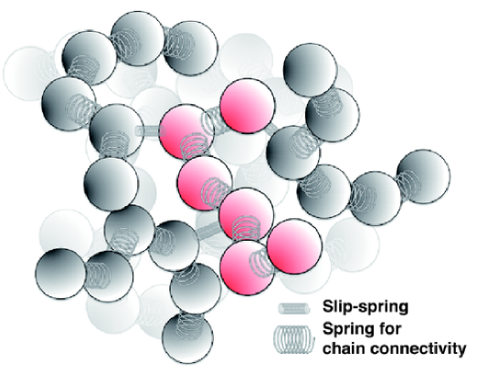
Figure 1: T. Uneyama and Y. Masubuchi to J. Chem. Phys

Figure 1 shows schematic view of the model employed in this study. We consider a network composed of bead-spring chains connected by slip-springs in a volume $V$. We describe the number of chains in the system as $M$, and the number of beads in a chain as $N$. The beads are connected along the chain backbone by linear entropic springs characterized by the average bond size $b$, and chains essentially behave as ideal, Rouse type chains. Apart from the chain connectivity, some of the beads are connected to the other beads by the slip-springs to mimic the entanglement between chains. Following the previous works[10, 11], we treat the degrees of freedom of slip-spring as state variables, which obey the Maxwell-Boltzmann type statistics in equilibrium. That is, we assume that the equilibrium probability distribution of the state variables is described by the Boltzmann weight with the (effective) free energy. The ends of slip-springs move (slip) along the chain to reproduce the chain slippage via entanglements. Instead of the continuous sliding dynamics proposed in the original single-chain model[10], we introduce the discrete hopping dynamics for the end of slip-spring between neighboring beads[11]. The slip-springs are stochastically destroyed when one of the ends is at the chain ends, and they are also stochastically constructed at the chain ends with a certain probability. For the spring force for slip-springs, we employ the linear entropic spring force (The strength of this entropic spring is characterized by the slip-spring parameter $N_{s}$.) It has been already pointed that slip-links or slip-springs effectively give attractive interaction between polymers and thus the statistical properties of polymer chains are affected by slip-springs[53]. We introduce a repulsive interaction between beads to compensate this attractive interaction induced by the slip-springs and to recover the ideal chain statistics. The number density of the slip-spring, $\phi$, is another parameter to control the strength of the entanglement effect, which is related to the entanglement density.

The state variables of the system are the position of beads, $\{\bm{R}_{i,k}\}$ (where $i$ and $k$ are the indices for chain and bead position on the chain, respectively), the total number of slip-springs in the system $Z$, and the connection matrix of slip-springs $\{\bm{S}_{\alpha}\}$ (where $\alpha$ is the index for slip-spring and the definition of $\bm{S}_{\alpha}$ is given later).

2.2 Equilibrium probability distribution

First we consider the equilibrium statistical properties. We assume that the chains in our multi-chain slip-spring system obey the ideal chain statistics. (There is no interaction between beads except the entropic linear springs.) Namely, the probability distribution for the polymer chain conformations $\{\bm{R}_{i,k}\}$ is given by

$$P_{\text{eq}}(\{\bm{R}_{i,k}\})=\frac{1}{V^{M}}\left(\frac{3}{2\pi b^{2}}\right)^{3M(N-1)/2}\exp\left[-\sum_{i=1}^{M}\sum_{k=1}^{N-1}\frac{3(\bm{R}_{i,k+1}-\bm{R}_{i,k})^{2}}{2b^{2}}\right]$$ (1)

Here the subscript “eq” represents the equilibrium quantity. $V$ is the volume of the system, $b$ is the bead size, $k_{B}$ is the Boltzmann constant, and $T$ is the temperature.

We consider to put slip-springs in the system, preserving the ideal chain statistics mentioned above. (As we mentioned, we assume that the system state, including the slip-springs, is characterized by the free energy.) For simplicity, we do not introduce restriction for the slip-spring configurations (connectivity). For example, we allow multiple slip-springs to share the same bead, or allow slip-springs to connect two beads on the same chain. Because both ends of a slip-spring are attached to beads, we need four indices to specify the state of a slip-spring. Hereafter, we describe the $k$-th bead on the $i$-th chain as $(i,k)$, and the state of the $\alpha$-th slip-spring as $\bm{S}_{\alpha}\equiv(S_{\alpha,1},S_{\alpha,2},S_{\alpha,3},S_{\alpha,4})$ where the ends of the slip-spring are located at the bead $(S_{\alpha,1},S_{\alpha,2})$ and the bead $(S_{\alpha,3},S_{\alpha,4})$.

We assume that there is no specific interaction between slip-springs. (This assumption is the same as one employed in single chain models, where slip-springs behave as one dimensional ideal gas[10, 11].) The number of slip-springs is not constant and it is controlled by the effective chemical potential for slip-springs[54]. Because slip-springs are statistically independent each other, for a given polymer conformation, the probability distribution of the slip-spring state is given by

$$P_{\text{eq}}(\{\bm{S}_{\alpha}\},Z|\{\bm{R}_{i,k}\})=\frac{1}{\Xi(\{\bm{R}_{i,k}\})}\frac{1}{Z!}\exp\bigg{[}-\sum_{\alpha=1}^{Z}\frac{3(\bm{R}_{S_{\alpha,1},S_{\alpha,2}}-\bm{R}_{S_{\alpha,3},S_{\alpha,4}})^{2}}{2N_{s}b^{2}}+\frac{\nu Z}{k_{B}T}\bigg{]}$$ (2)

where $P(X|Y)$ represents the conditional probability of $X$ under a given $Y$, $Z$ is the total number of slip-springs in the system, and $N_{s}$ is the parameter related to the spring constant of slip-spring, and $\nu$ is the effective chemical potential for slip-springs. $\Xi(\{\bm{R}_{i,k}\})$ is the grand partition function of the slip-spring defined as

$$\Xi(\{\bm{R}_{i,k}\})\equiv\sum_{Z=0}^{\infty}\sum_{\{\bm{S}_{\alpha}\}}\frac{1}{Z!}\exp\bigg{[}-\sum_{\alpha=1}^{Z}\frac{3(\bm{R}_{S_{\alpha,1},S_{\alpha,2}}-\bm{R}_{S_{\alpha,3},S_{\alpha,4}})^{2}}{2N_{s}b^{2}}+\frac{\nu Z}{k_{B}T}\bigg{]}$$ (3)

Here $\sum_{\{\bm{S}_{\alpha}\}}$ is taken for all possible slip-spring indices. Eq (3) can be calculated as follows.

$$\begin{split}\Xi(\{\bm{R}_{i,k}\})&=\sum_{Z=0}^{\infty}\frac{1}{Z!}\bigg{[}e^{\nu/k_{B}T}\sum_{\bm{S}}\exp\bigg{[}-\frac{3(\bm{R}_{S_{1},S_{2}}-\bm{R}_{S_{3},S_{4}})^{2}}{2N_{s}b^{2}}\bigg{]}\bigg{]}^{Z}\\ &=\exp\bigg{[}e^{\nu/k_{B}T}\sum_{\bm{S}}\exp\bigg{[}-\frac{3(\bm{R}_{S_{1},S_{2}}-\bm{R}_{S_{3},S_{4}})^{2}}{2N_{s}b^{2}}\bigg{]}\bigg{]}\\ &=\exp\bigg{[}e^{\nu/k_{B}T}\sum_{i,k,j,l}\exp\bigg{[}-\frac{3(\bm{R}_{i,k}-\bm{R}_{j,l})^{2}}{2N_{s}b^{2}}\bigg{]}\bigg{]}\end{split}$$ (4)

Substituting eq (4) into eq (2), we obtain

$$\begin{split}P_{\text{eq}}(\{\bm{S}_{\alpha}\},Z|\{\bm{R}_{i,k}\})&=\frac{1}{Z!}\exp\bigg{[}-e^{\nu/k_{B}T}\sum_{i,k,j,l}\exp\bigg{[}-\frac{3(\bm{R}_{i,k}-\bm{R}_{j,l})^{2}}{2N_{s}b^{2}}\bigg{]}\\ &\qquad-\sum_{\alpha=1}^{Z}\frac{3(\bm{R}_{S_{\alpha,1},S_{\alpha,2}}-\bm{R}_{S_{\alpha,3},S_{\alpha,4}})^{2}}{2N_{s}b^{2}}+\frac{\nu Z}{k_{B}T}\bigg{]}\end{split}$$ (5)

Eqs (1) and (5) give the equilibrium distribution function of the full set of state variables as

$$\begin{split}P_{\text{eq}}(\{\bm{R}_{i,k}\},\{\bm{S}_{\alpha}\},Z)&=\frac{1}{Z!}\frac{1}{V^{M}}\left(\frac{3}{2\pi b^{2}}\right)^{3M(N-1)/2}\exp\bigg{[}\frac{\nu Z}{k_{B}T}-\sum_{i,k}\frac{3(\bm{R}_{i,k+1}-\bm{R}_{i,k})^{2}}{2b^{2}}\\ &\qquad-\sum_{\alpha=1}^{Z}\frac{3(\bm{R}_{S_{\alpha,1},S_{\alpha,2}}-\bm{R}_{S_{\alpha,3},S_{\alpha,4}})^{2}}{2N_{s}b^{2}}\\ &\qquad-e^{\nu/k_{B}T}\sum_{i,k,j,l}\exp\left[-\frac{3(\bm{R}_{i,k}-\bm{R}_{j,l})^{2}}{2N_{s}b^{2}}\right]\bigg{]}\end{split}$$ (6)

The effective free energy corresponds to eq (6) is given by

$$\begin{split}\frac{\mathcal{F}(\{\bm{R}_{i,k}\},\{\bm{S}_{\alpha}\},Z)}{k_{B}T}&=\sum_{i,k}\frac{3(\bm{R}_{i,k+1}-\bm{R}_{i,k})^{2}}{2b^{2}}+\sum_{\alpha=1}^{Z}\frac{3(\bm{R}_{S_{\alpha,1},S_{\alpha,2}}-\bm{R}_{S_{\alpha,3},S_{\alpha,4}})^{2}}{2N_{s}b^{2}}\\ &\qquad+e^{\nu/k_{B}T}\sum_{i,k,j,l}\exp\left[-\frac{3(\bm{R}_{i,k}-\bm{R}_{j,l})^{2}}{2N_{s}b^{2}}\right]\end{split}$$ (7)

The free energy (7) consists of several contributions. The first and second terms in the right hand side of eq (7) are the elastic energies of polymer chains and slip-springs, respectively. The third term in the right hand side of eq (7) represents the repulsive interaction which compensates the attractive interaction caused by slip-springs[53]. The repulsive potential is a soft-core Gaussian type and similar to the Flory-Krigbaum potential[55]. However, it should be emphasized that this repulsive interaction is not introduced to reproduce the excluded volume effect and the overlapping among the chains, but to compensate the artificial attraction by slip-springs. Indeed, the Gaussian form comes from the harmonic potential of slip-springs. This repulsive interaction acts not only for the beads connected to slip-springs but also for the free beads. Using the effective free energy given by (7), eq (6) can be rewritten as

$$\begin{split}P_{\text{eq}}(\{\bm{R}_{i,k}\},\{\bm{S}_{\alpha}\},Z)&=\frac{1}{Z!}\frac{1}{V^{M}}\left(\frac{3}{2\pi b^{2}}\right)^{3M(N-1)/2}\exp\bigg{[}\frac{\nu Z}{k_{B}T}-\frac{\mathcal{F}(\{\bm{R}_{i,k}\},\{\bm{S}_{\alpha}\},Z)}{k_{B}T}\bigg{]}\end{split}$$ (8)

The equilibrium statistical average, which we describe as $\langle\dots\rangle_{\text{eq}}$, can be defined as

$$\langle\dotsb\rangle_{\text{eq}}\equiv\int d\{\bm{R}_{i,k}\}\,\sum_{Z=0}^{\infty}\sum_{\{\bm{S}_{\alpha}\}}\dotsb P_{\text{eq}}(\{\bm{R}_{i,k}\},\{\bm{S}_{\alpha}\},Z)$$ (9)

In our model, the number of slip-springs is controlled by the effective chemical potential $\nu$. However, in practice, the effective chemical potential is not convenient nor intuitive. Thus, instead of $\nu$, we utilize the average number density of slip-springs, $\phi$ as an input parameter. (In the thermodynamic limit where $M,V\to\infty$ with fixed $\rho_{0}$, the average slip-spring number $\langle Z\rangle_{\text{eq}}=\phi V$ becomes an extensive variable while $\phi$ is an intensive variable.) The equilibrium average number density of slip-springs can be calculated from the equilibrium probability distribution given by (6).

$$\begin{split}\phi&\equiv\langle Z/V\rangle_{\text{eq}}\\ &=\frac{1}{V}\int d\{\bm{R}_{i,k}\}\,\sum_{Z=0}^{\infty}\sum_{\{\bm{S}_{\alpha}\}}ZP_{\text{eq}}(\{\bm{R}_{i,k}\},\{\bm{S}_{\alpha}\},Z)\\ &=\frac{e^{\nu/k_{B}T}}{V}\int d\{\bm{R}_{i,k}\}\,\sum_{i,k,j,l}\exp\bigg{[}-\frac{3(\bm{R}_{i,k}-\bm{R}_{j,l})^{2}}{2N_{s}b^{2}}\bigg{]}P_{\text{eq}}(\{\bm{R}_{i,k}\})\\ &=\frac{e^{\nu/k_{B}T}}{V}\int d\bm{r}\,e^{-3\bm{r}^{2}/2N_{s}b^{2}}\bigg{\langle}\sum_{i,k,j,l}\delta(\bm{R}_{i,k}-\bm{R}_{j,k}-\bm{r})\bigg{\rangle}_{\text{eq}}\end{split}$$ (10)

To evaluate $\phi$, the pair-correlation function of beads is required. This pair correlation function can be calculated straightforwardly, since there is no correlation between different chains. Thus we have

$$\begin{split}\bigg{\langle}\sum_{i,k,j,l}\delta(\bm{R}_{i,k}-\bm{R}_{j,k}-\bm{r})\bigg{\rangle}_{\text{eq}}&=M\bigg{\langle}\sum_{k,l}\delta(\bm{R}_{i,k}-\bm{R}_{i,l}-\bm{r})\bigg{\rangle}_{\text{eq}}+\frac{M(M-1)N^{2}}{V^{2}}\\ &=\frac{M}{V}\sum_{k,l}\left(\frac{3}{2\pi|k-l|b^{2}}\right)^{3/2}\exp\bigg{(}-\frac{3\bm{r}^{2}}{2|k-l|b^{2}}\bigg{)}+\frac{M(M-1)N^{2}}{V^{2}}\end{split}$$ (11)

Substituting eq (11) into eq (10), we have

$$\phi=\rho_{0}e^{\nu/k_{B}T}\bigg{[}1+\frac{2}{N}\sum_{k=1}^{N}\sum_{l=1}^{k-1}\bigg{(}\frac{N_{s}}{k-l+N_{s}}\bigg{)}^{3/2}+\bigg{(}\rho_{0}-\frac{N}{V}\bigg{)}\bigg{(}\frac{2\pi N_{s}b^{2}}{3}\bigg{)}^{3/2}\bigg{]}$$ (12)

Here, $\rho_{0}\equiv MN/V$ is the average number density of beads. Eq (12) indicates that the average slip-spring number depends not only on the effective chemical potential but also on the bead density $\rho_{0}$ and the slip-spring intensity $N_{s}$. This is different from the single chain slip-spring model where the slip-spring density is depends only on the chemical potential $\nu$ [11]. From eq (12), the effective chemical potential $\nu$ corresponding to a given $\phi$ is obtained as

$$\nu=-k_{B}T\ln\bigg{[}\frac{\rho_{0}}{\phi}\bigg{[}1+\frac{2}{N}\sum_{k=1}^{N}\sum_{l=1}^{k-1}\bigg{(}\frac{N_{s}}{k-l+N_{s}}\bigg{)}^{3/2}+\bigg{(}\rho_{0}-\frac{N}{V}\bigg{)}\bigg{(}\frac{2\pi N_{s}b^{2}}{3}\bigg{)}^{3/2}\bigg{]}\bigg{]}$$ (13)

To calculate rheological properties, we need expression of the stress tensor of the system. In this work, we employ the following definition for the stress tensor according to the stress-optical law.

$$\hat{\bm{\sigma}}\equiv\frac{1}{V}\bigg{[}\sum_{i,k}\frac{3k_{B}T}{b^{2}}(\bm{R}_{i,k+1}-\bm{R}_{i,k})(\bm{R}_{i,k+1}-\bm{R}_{i,k})-MNk_{B}T\bm{1}\bigg{]}$$ (14)

Here $\bm{1}$ is unit tensor. In equilibrium, eq (14) reduces to the following form.

$$\begin{split}\langle\hat{\bm{\sigma}}\rangle_{\text{eq}}&=-\frac{M}{V}k_{B}T\bm{1}\end{split}$$ (15)

This is the stress tensor of ideal gas, of which number density is $M/V$. The definition of the stress tensor in a slip-spring type model is not trivial. It is possible to include the contributions from the slip-springs (contributions from the elastic force and the repulsive force). Fortunately, most of rheological properties seem to be not sensitive to the definition of the stress tensor, at least qualitatively[11, 53]. We will discuss another possible definition of the stress tensor, later.

2.3 Dynamics

While we have specified the equilibrium probability distribution in the previous section, the dynamical properties such as the viscoelasticity cannot be determined unless the time evolution equations (rules) for the state variables are specified. In this section, we design time evolution equations which satisfy the detailed balance condition. (The detailed balance condition is required to be satisfied to reproduce the equilibrium thermodynamical properties correctly.) There are many possible time evolution equations (rules) which satisfy the detailed balance condition, and thus we cannot uniquely determine the dynamical model solely by the equilibrium probability distribution and the detailed balance condition. In this work, we propose a simple dynamics model which is similar to the single chain slip-spring models[10, 11] and suitable for numerical simulations.

First, for the time evolution of the bead position $\bm{R}_{i,k}$, we employ an overdamped Langevin type equation of motion. In absence of the external deformation field, the dynamic equation is given as follows.

$$\frac{d\bm{R}_{i,k}(t)}{dt}=-\frac{1}{\zeta}\frac{\partial\mathcal{F}(\{\bm{R}_{i,k}\},\{\bm{S}_{\alpha}\},Z)}{\partial\bm{R}_{i,k}}+\bm{\xi}_{i,k}(t)$$ (16)

Here $\zeta$ is the friction coefficient of a bead and $\bm{\xi}_{i,k}(t)$ is the Gaussian noise obeying the fluctuation dissipation relation of the second kind;

$$\langle\bm{\xi}_{i,k}(t)\rangle=0$$ (17)

$$\langle\bm{\xi}_{i,k}(t)\bm{\xi}_{j,l}(t^{\prime})\rangle=\frac{2k_{B}T}{\zeta}\delta_{ij}\delta_{kl}\delta(t-t^{\prime})\bm{1}$$ (18)

where $\langle\dotsb\rangle$ represents the statistical average. For some analyses, it would be convenient to introduce the Fokker-Planck equation. The Fokker-Plank equation which corresponds to eq (16) is

$$\begin{split}\frac{\partial P(\{\bm{R}_{i,k}\},\{\bm{S}_{\alpha}\},Z;t)}{\partial t}&=\sum_{i,k}\frac{1}{\zeta}\frac{\partial}{\partial\bm{R}_{i,k}}\cdot\left[\frac{\partial\mathcal{F}(\{\bm{R}_{i,k}\},\{\bm{S}_{\alpha}\},Z)}{\partial\bm{R}_{i,k}}P+k_{B}T\frac{\partial P}{\partial\bm{R}_{i,k}}\right]\\ &\equiv\mathcal{L}_{\text{FP}}P\end{split}$$ (19)

Here $P(\{\bm{R}_{i,k}\},\{\bm{S}_{\alpha}\},Z;t)$ is the time dependent probability distribution and $\mathcal{L}_{\text{FP}}$ is the Fokker-Planck operator. It is clear that eq (19) satisfies the detailed balance condition and the steady state distribution coincides to the equilibrium distribution given by eq (6).

Second, we consider the reconstruction process of slip-springs. We assume that the reconstructions of slip-springs are independent of each other, and the positions of polymers and other slip-springs do not change during the reconstruction process. We write the construction rate of a new slip-spring as $W_{+}(\bm{S}_{Z},Z|Z-1)$ and the destruction rate of the $\beta$-th slip-spring as $W_{-}(Z-1|\bm{S}_{\beta},Z)$. We assume that a slip-spring is destroyed with a certain fixed probability when one of its ends is at the chain ends. The destruction rate can be written as

$$W_{-}(Z-1|\bm{S}_{\beta},Z)=\frac{k_{B}T}{\zeta_{s}}\left[\delta_{S_{Z,2},1}+\delta_{S_{Z,2},N}+\delta_{S_{Z,4},1}+\delta_{S_{Z,4},N}\right]\mathcal{E}(\beta,Z)$$ (20)

Here, $\zeta_{s}$ is the friction coefficient of a slip-spring and $\mathcal{E}(\beta,Z)$ is the exchange operator which exchange the $\beta$-th and $Z$-th slip-springs. (By operating $\mathcal{E}(\beta,Z)$, $\bm{S}_{\beta}$ and $\bm{S}_{Z}$ are exchanged while the other slip-spring indices are unchanged. This operator is employed to ensure that the $Z$-th slip-spring is always destroyed.)

The slip-spring construction and destruction processes should be detailed-balanced. The detailed balance condition can be explicitly written as follows.

$$W_{+}(\bm{S}_{Z},Z|Z-1)P_{\text{eq}}(\{\bm{R}_{i,k}\},\{\bm{S}_{\alpha}\},Z-1)=\sum_{\beta=1}^{Z}W_{-}(Z-1|\bm{S}_{\beta},Z)P_{\text{eq}}(\{\bm{R}_{i,k}\},\{\bm{S}_{\alpha}\},Z)$$ (21)

From eqs (20) and (21), the construction rate is uniquely determined. By substituting eq (20) into eq (21), we obtain the following explicit form for the construction rate.

$$\begin{split}W_{+}(\bm{S}_{Z},Z|Z-1)&=\frac{1}{P_{\text{eq}}(\{\bm{R}_{i,k}\},\{\bm{S}_{\alpha}\},Z-1)}\sum_{\beta=1}^{Z}W_{-}(Z-1|\bm{S}_{\beta},Z)P_{\text{eq}}(\{\bm{R}_{i,k}\},\{\bm{S}_{\alpha}\},Z)\\ &=\frac{k_{B}T}{\zeta_{s}}\left[\delta_{S_{Z,2},1}+\delta_{S_{Z,2},N}+\delta_{S_{Z,4},1}+\delta_{S_{Z,4},N}\right]e^{\nu/k_{B}T}\\ &\qquad\times\exp\bigg{[}-\frac{3(\bm{R}_{S_{Z,1},S_{Z,2}}-\bm{R}_{S_{Z,3},S_{Z,4}})^{2}}{2N_{s}b^{2}}\bigg{]}\end{split}$$ (22)

As before, it would be convenient to introduce the dynamic equation for the time dependent probability distribution. The master equation for this reconstruction is written as

$$\begin{split}\frac{\partial P(\{\bm{R}_{i,k}\},\{\bm{S}_{\alpha}\},Z;t)}{\partial t}&=\sum_{\beta=1}^{Z+1}W_{-}(Z|\bm{S}_{\beta},Z+1)P(Z+1)+W_{+}(\bm{S}_{Z},Z|Z-1)P(Z-1)\\ &\qquad-\sum_{\beta=1}^{Z}W_{-}(Z-1|\bm{S}_{\beta},Z)P(Z)\\ &\qquad-\int d\bm{S}_{Z+1}\,W_{+}(\bm{S}_{Z+1},Z+1|Z)P(Z)\\ &\equiv\mathcal{L}_{\text{rc}}P\end{split}$$ (23)

where we have introduced the time evolution operator for the reconstruction process $\mathcal{L}_{\text{rc}}$.

Finally, we consider the hopping of slip-springs along the chain. We assume that there is no interaction between slip-springs and each hopping event is statistically independent. The hopping process can be described by the change of connectivity index. For simplicity, we also assume that the change of connectivity index is restricted as $\pm 1$. (Namely, in our model, the hopping distance of slip-spring on a chain corresponds to the bead size). We consider the event where the $\beta$-th slip-spring changes its connectivity from $\bm{S}_{\beta}$ to $\bm{S}^{\prime}_{\beta}$. We describe the set of slip-spring indices after the hopping as $\{\bm{S}^{\prime}_{\alpha}\}$, for convenience. $\bm{S}^{\prime}_{\alpha}$ is defined as

$$\bm{S}_{\alpha}^{\prime}=\begin{cases}\bm{S}_{\beta}^{\prime}&(\alpha=\beta)\\ \bm{S}_{\alpha}&(\text{otherwise})\end{cases}$$ (24)

Let us indicate the transition rate of $\beta$-th slip-spring from $\bm{S}_{\beta}$ to $\bm{S}_{\beta}^{\prime}$ as $W(\bm{S}^{\prime}_{\beta}|\bm{S}_{\beta})$ and its transition rate of the inverse process as $W(\bm{S}_{\beta}|\bm{S}^{\prime}_{\beta})$. The detailed balance condition can be written as

$$\begin{split}\frac{W(\bm{S}^{\prime}_{\beta}|\bm{S}_{\beta})}{W(\bm{S}_{\beta}|\bm{S}^{\prime}_{\beta})}&=\frac{P_{\text{eq}}(\{\bm{R}_{i,k}\},\{\bm{S}_{\alpha}^{\prime}\},Z)}{P_{\text{eq}}(\{\bm{R}_{i,k}\},\{\bm{S}_{\alpha}\},Z)}\\ &=\exp\bigg{[}-\frac{3(\bm{R}_{S_{\beta,1}^{\prime},S_{\beta,2}^{\prime}}-\bm{R}_{S_{\beta,3}^{\prime},S_{\beta,4}^{\prime}})^{2}}{2N_{s}b^{2}}+\frac{3(\bm{R}_{S_{\beta,1},S_{\beta,2}}-\bm{R}_{S_{\beta,3},S_{\beta,4}})^{2}}{2N_{s}b^{2}}\bigg{]}\end{split}$$ (25)

If we employ the Glauber type dynamics for the hopping process[56], the transition rate which satisfies eq (25) can be expressed as follows.

$$\begin{split}W(\bm{S}_{\beta}^{\prime}|\bm{S}_{\beta})&=\frac{k_{B}T}{\zeta_{s}}\delta_{S_{\beta,1},S_{\beta,1}^{\prime}}\delta_{S_{\beta,3},S_{\beta,3}^{\prime}}\bigg{[}\left(\delta_{S_{\beta,2},S_{\beta,2}^{\prime}-1}+\delta_{S_{\beta,2},S_{\beta,2}^{\prime}+1}\right)\delta_{S_{\beta,4},S_{\beta,4}^{\prime}}\\ &\qquad+\left(\delta_{S_{\beta,4},S_{\beta,4}^{\prime}-1}+\delta_{S_{\beta,4},S_{\beta,4}^{\prime}+1}\right)\delta_{S_{\beta,2},S_{\beta,2}^{\prime}}\bigg{]}\left[1-\tanh\frac{\Delta\mathcal{F}_{\text{hop}}(\bm{S}_{\beta}^{\prime};\bm{S}_{\beta})}{2k_{B}T}\right]\end{split}$$ (26)

$$\frac{\Delta\mathcal{F}_{\text{hop}}(\bm{S}_{\beta}^{\prime};\bm{S}_{\beta})}{k_{B}T}\equiv\frac{3}{2N_{s}b^{2}}\left[(\bm{R}_{S_{\beta,1}^{\prime},S_{\beta,2}^{\prime}}-\bm{R}_{S_{\beta,3}^{\prime},S_{\beta,4}^{\prime}})^{2}-(\bm{R}_{S_{\beta,1},S_{\beta,2}}-\bm{R}_{S_{\beta,3},S_{\beta,4}})^{2}\right]$$ (27)

The master equation for the hopping can be written as

$$\begin{split}\frac{\partial P(\{\bm{R}_{i,k}\},\{\bm{S}_{\alpha}\},Z;t)}{\partial t}&=\sum_{\beta=1}^{Z}\sum_{\bm{S}_{\beta}^{\prime}}\big{[}W(\bm{S}_{\beta}|\bm{S}_{\beta}^{\prime})P(\{\bm{S}_{\alpha}^{\prime}\})-W(\bm{S}_{\beta}^{\prime}|\bm{S}_{\beta})P(\{\bm{S}_{\alpha}\})\big{]}\\ &\equiv\mathcal{L}_{\text{hop}}P\end{split}$$ (28)

Here we have introduced the time evolution operator for the hopping process $\mathcal{L}_{\text{hop}}$.

Full dynamics of the system is then described by the Langevin equation given by eq (16), the reconstruction process (with the reconstruction rates (20) and (22)), and the hopping process (with the hopping rate (26)). All of these processes satisfy the detailed balance condition, and thus it is clear that the equilibrium state is realized as characterized by the probability distribution (8). The master equation of the system is expressed by combining the Fokker-Planck and master equations, (19), (23), and (28).

$$\frac{\partial P(\{\bm{R}_{i,k}\},\{\bm{S}_{\alpha}\},Z;t)}{\partial t}=\left[\mathcal{L}_{\text{FP}}+\mathcal{L}_{\text{rc}}+\mathcal{L}_{\text{hop}}\right]P(\{\bm{R}_{i,k}\},\{\bm{S}_{\alpha}\},Z;t)$$ (29)

2.4 Relaxation modulus

In this section, we will derive an explicit expression of the relaxation modulus tensor from the equilibrium distribution (eq (8)) and the master equation (eq (29)) via the linear response theory[57].

We consider the system is subjected to the weak external deformation field, which is characterized by the time-dependent velocity gradient tensor $\bm{\kappa}(t)$. Such a deformation gives an additional term to the master equation (29), which will be treated as a perturbation in the followings. By adding the perturbation term, the master equation (29) is modified as

$$\frac{\partial P(\{\bm{R}_{i,k}\},\{\bm{S}_{\alpha}\},Z;t)}{\partial t}=\left[\mathcal{L}_{0}+\mathcal{L}_{1}(t)\right]P(\{\bm{R}_{i,k}\},\{\bm{S}_{\alpha}\},Z;t)$$ (30)

where $\mathcal{L}_{0}$ and $\mathcal{L}_{1}(t)$ are the equilibrium and perturbation time evolution operators.

$$\mathcal{L}_{0}\equiv\mathcal{L}_{\text{FP}}+\mathcal{L}_{\text{rc}}+\mathcal{L}_{\text{hop}}$$ (31)

$$\mathcal{L}_{1}(t)P\equiv-\sum_{i,k}\frac{\partial}{\partial\bm{R}_{i,k}}\cdot\left[\bm{\kappa}(t)\cdot\bm{R}_{i,k}P\right]$$ (32)

As we mentioned, our dynamics model satisfies the detailed balance condition and thus the following relation holds for $\mathcal{L}_{0}$ and the equilibrium distribution (8).

$$\mathcal{L}_{0}P_{\text{eq}}(\{\bm{R}_{i,k}\},\{\bm{S}_{\alpha}\},Z)=0$$ (33)

Up to the first order in the perturbation, eq (30) can be formally integrated as

$$P(\{\bm{R}_{i,k}\},\{\bm{S}_{\alpha}\},Z;t)=P_{\text{eq}}(\{\bm{R}_{i,k}\},\{\bm{S}_{\alpha}\},Z)+\int_{-\infty}^{t}dt^{\prime}\,e^{(t-t^{\prime})\mathcal{L}_{0}}\left[\mathcal{L}_{1}(t^{\prime})P_{\text{eq}}(\{\bm{R}_{i,k}\},\{\bm{S}_{\alpha}\},Z)\right]$$ (34)

Then the ensemble average of the stress tensor at time $t$, $\bm{\sigma}(t)$, can be written as

$$\begin{split}\bm{\sigma}(t)&=\int d\{\bm{R}_{i,k}\}\sum_{Z=0}^{\infty}\sum_{\{\bm{S}_{\alpha}\}}\hat{\bm{\sigma}}P(\{\bm{R}_{i,k}\},\{\bm{S}_{\alpha}\},Z;t)\\ &=\langle\hat{\bm{\sigma}}\rangle_{\text{eq}}+\frac{1}{k_{B}T}\int_{-\infty}^{t}dt^{\prime}\,\bigg{\langle}\hat{\bm{\sigma}}(t-t^{\prime})\sum_{i,k}\bigg{[}\frac{\partial\mathcal{F}(\{\bm{R}_{i,k}\},\{\bm{S}_{\alpha}\},Z)}{\partial\bm{R}_{i,k}}\bm{R}_{i,k}-k_{B}T\bm{1}\bigg{]}\bigg{\rangle}_{\text{eq}}:\bm{\kappa}(t^{\prime})\\ &=\langle\hat{\bm{\sigma}}\rangle_{\text{eq}}+\frac{V}{k_{B}T}\int_{-\infty}^{t}dt^{\prime}\,\big{\langle}\hat{\bm{\sigma}}(t-t^{\prime})[\hat{\bm{\sigma}}+\hat{\bm{\sigma}}^{(v)}]\big{\rangle}_{\text{eq}}:\bm{\kappa}(t^{\prime})\end{split}$$ (35)

Here we have defined the time shifted operator as $\hat{\bm{\sigma}}(t)\equiv e^{t\mathcal{L}_{0}^{\dagger}}\hat{\bm{\sigma}}$ ($\mathcal{L}_{0}^{\dagger}$ is the adjoint operator for $\mathcal{L}_{0}$). This represents the stress tensor at time $t$ after the reference time. Also, we have defined the virtual stress operator $\hat{\bm{\sigma}}^{(v)}$ as

$$\begin{split}\hat{\bm{\sigma}}^{(v)}&\equiv\frac{1}{V}\bigg{[}\sum_{\alpha=1}^{Z}\frac{3k_{B}T}{N_{s}b^{2}}(\bm{R}_{S_{\alpha,1},S_{\alpha,2}}-\bm{R}_{S_{\alpha,3},S_{\alpha,4}})(\bm{R}_{S_{\alpha,1},S_{\alpha,2}}-\bm{R}_{S_{\alpha,3},S_{\alpha,4}})\\ &\qquad-e^{\nu/k_{B}T}\sum_{i,k,j,l}\frac{3k_{B}T}{N_{s}b^{2}}(\bm{R}_{i,k}-\bm{R}_{j,l})(\bm{R}_{i,k}-\bm{R}_{j,l})\exp\left[-\frac{3(\bm{R}_{i,k}-\bm{R}_{j,l})^{2}}{2N_{s}b^{2}}\right]\bigg{]}\end{split}$$ (36)

The virtual stress represents the stress generated by slip-springs and the repulsive interaction between beads. The relaxation modulus tensor $\bm{G}(t)$ (which is a fourth order tensor) can be defined for a small deformation as follows.

$$\bm{\sigma}(t)-\langle\hat{\bm{\sigma}}\rangle_{\text{eq}}\equiv\int_{-\infty}^{t}dt^{\prime}\,\bm{G}(t-t^{\prime}):\bm{\kappa}(t^{\prime})$$ (37)

By comparing eqs (35) and (37), we obtain

$$\bm{G}(t)=\frac{V}{k_{B}T}\big{\langle}\hat{\bm{\sigma}}(t)\big{[}\hat{\bm{\sigma}}+\hat{\bm{\sigma}}^{(v)}\big{]}\big{\rangle}_{\text{eq}}$$ (38)

Eq (38) is similar to the linear response formula obtained for single chain models[31, 11] where the necessity of the virtual stress tensor is already known. However, the explicit form of the virtual stress tensor (36) differs from one for single chain models. In our model, the virtual stress tensor has the contribution from the repulsive interaction between beads. Physically this is natural because the repulsive interaction originates as the compensation of the attractive interaction by the slip-springs.

In eq (38), we assume that only the stress tensor $\hat{\bm{\sigma}}$ represents the stress tensor of the system (eq (14)). As we mentioned, this assumption is based on the stress-optical law, which is empirically known to hold for various polymeric materials. However, from the view point of the virtual work method, it is also possible to employ $\hat{\bm{\sigma}}+\hat{\bm{\sigma}}^{(v)}$ (which is conjugate to the deformation) as the stress tensor of the system. If we employ the latter expression, the ensemble average in eq (38) is replaced by $\langle[\hat{\bm{\sigma}}(t)+\hat{\bm{\sigma}}^{(v)}(t)][\hat{\bm{\sigma}}+\hat{\bm{\sigma}}^{(v)}]\rangle_{\text{eq}}$. Then we have the following formula.

$$\bm{G}(t)=\frac{V}{k_{B}T}\big{\langle}\big{[}\hat{\bm{\sigma}}(t)+\hat{\bm{\sigma}}^{(v)}(t)\big{]}\big{[}\hat{\bm{\sigma}}+\hat{\bm{\sigma}}^{(v)}\big{]}\big{\rangle}_{\text{eq}}$$ (39)

(In the single chain slip-spring model, both of these two different expressions give qualitatively similar relaxation moduli.[11] We expect that the situation is similar in our multi chain model.) We will compare simulation results for eqs (39) and (39), later.

2.5 Numerical scheme

In this section, we show a numerical scheme for simulations based on our multi-chain slip-spring model. We choose the bead size $b$, $k_{B}T$, and $\zeta$ as the unit of length, energy, and friction (so that the unit of time is $\tau_{0}=\zeta b^{2}/k_{B}T$). In the followings we set $b=1$, $k_{B}T=1$, and $\zeta=1$. By using the operator-splitting method, the formal solution of eq (29) can be approximated as

$$P(\{\bm{R}_{i,k}\},\{\bm{S}_{\alpha}\},Z;t+\Delta t)\approx e^{\Delta t\mathcal{L}_{\text{rc}}}e^{\Delta t\mathcal{L}_{\text{hop}}}e^{\Delta t\mathcal{L}_{\text{FP}}}P(\{\bm{R}_{i,k}\},\{\bm{S}_{\alpha}\},Z;t)$$ (40)

Eq (40) corresponds to a numerical scheme with three substeps and the integration time step $\Delta t$. That is, the time evolution from time $t$ to time $t+\Delta t$ is simulated by performing the Langevin dynamics of the beads, the hopping dynamics of the slip-springs, and the reconstruction of the slip-springs. (These steps are iterated sequentially.)

For the integration of the Langevin equation, we employ the explicit Euler scheme. The Langevin equation for the chain dynamics can be discretized as

$$\bm{R}_{i,k}(t+\Delta t)\approx-\Delta t\frac{\partial\mathcal{F}(\{\bm{R}_{i,k}\},\{\bm{S}_{\alpha}\},Z)}{\partial\bm{R}_{i,k}}+\sqrt{2\Delta t}\bm{w}_{i,k}$$ (41)

Here $\bm{w}_{i,k}$ is the Gaussian random number vector.

The hopping dynamics of slip-spring is described by the change of slip-spring indices as mentioned above. When $\Delta t$ is sufficiently small, the index of the $\alpha$-th slip-spring, $S_{\alpha,\lambda}$ ($\lambda=2,4$) is changed as $S_{\alpha,\lambda}\to S_{\alpha,\lambda}\pm 1$ by the following cumulative probability.

$$\Psi_{\lambda\pm}=\frac{\Delta t}{\zeta_{s}}\left[1-\tanh\frac{\Delta\mathcal{F}_{\lambda\pm}}{2}\right]\qquad(\lambda=2,4)$$ (42)

Here $\Delta\mathcal{F}_{\lambda\pm}$ is the free energy difference given by

$$\Delta\mathcal{F}_{2\pm}\equiv\frac{3}{2N_{s}}\left[(\bm{R}_{S_{\alpha,1},S_{\alpha,2}\pm 1}-\bm{R}_{S_{\alpha,3},S_{\alpha,4}})^{2}-(\bm{R}_{S_{\alpha,1},S_{\alpha,2}}-\bm{R}_{S_{\alpha,3},S_{\alpha,4}})^{2}\right]$$ (43)

$$\Delta\mathcal{F}_{4\pm}\equiv\frac{3}{2N_{s}}\left[(\bm{R}_{S_{\alpha,1},S_{\alpha,2}}-\bm{R}_{S_{\alpha,3},S_{\alpha,4}\pm 1})^{2}-(\bm{R}_{S_{\alpha,1},S_{\alpha,2}}-\bm{R}_{S_{\alpha,3},S_{\alpha,4}})^{2}\right]$$ (44)

The reconstruction of the slip-springs is performed as follows. When an end of the $\alpha$-th slip-spring is at a chain end, the slip-spring is destroyed with the following cumulative probability.

$$\Psi_{-}=\frac{\Delta t}{\zeta_{s}}$$ (45)

When the slip-spring is destroyed, the index $\alpha$ for the other slip-springs is rearranged to realize $\alpha=1,2,3,\dots,Z$ without vacant number. (This rearrangement is expressed by the exchange operator in eq (20).) After the attempts of destruction for all slip-springs, construction of a new slip-spring is attempted. This construction step is made by a Monte Carlo sampling scheme. A new slip-spring is virtually generated and its end is attached to a chain end. Another end is attached to one of the surrounding beads which is chosen randomly. Thus a new slip-spring index $\bm{S}$ is generated. This virtual slip-spring is accepted as a newly generated slip-spring with the following probability.

$$\Psi_{+}=\exp\left[-\frac{3(\bm{R}_{S_{1},S_{2}}-\bm{R}_{S_{3},S_{4}})^{2}}{2N_{s}}\right]$$ (46)

If accepted, we set $\bm{S}_{Z+1}=\bm{S}$ and increase $Z\to Z+1$. This Monte Carlo sampling is made for

$$\bar{K}\equiv 4M^{2}N\frac{\Delta t}{\zeta_{s}}e^{\nu}$$ (47)

times on average, where the factor $4M^{2}N$ is the total number of possible connections factorized by the number of ends for a slip-spring, 2, the total number of chain ends, $2M$, and the total number of beads, $MN$. As a simple scheme, we assume that $K$ only takes the floor or ceiling of $\bar{K}$, ($\lfloor\bar{K}\rfloor$ or $\lceil\bar{K}\rceil$). The probability that we have $K$ trials at a certain construction step is given by

$$P(K=\lfloor\bar{K}\rfloor)=\lceil\bar{K}\rceil-\bar{K}$$ (48)

$$P(K=\lceil\bar{K}\rceil)=\bar{K}-\lfloor\bar{K}\rfloor=1-P(K=\lfloor\bar{K}\rfloor)$$ (49)

This guarantees that the average sampling number becomes $\langle K\rangle=\bar{K}$, and the numbers of the slip-spring construction and destruction balance in equilibrium.

The number of Monte Carlo sampling for construction can be significantly reduced if we exclude the constructions for very low acceptance probabilities. The acceptance probability decreases considerably if the stretch of a slip-spring becomes large. Thus, we limit the newly constructed slip-springs to be sampled only inside a certain cut-off size. We introduce a cut-off $r_{c}\equiv\sqrt{C_{0}^{2}N_{s}/3}$ to restrict the sampling for construction of slip-spring with its length shorter than $r_{c}$. The cut-off parameter $C_{0}$ is determined to obey $e^{-C_{0}^{2}/2}\ll 1$ and practically this condition is satisfied if $C_{0}\gtrsim 3$. The average number of trials for every $\Delta t$ is written as

$$\bar{K}=4M\tilde{N}_{0}(C_{0})\frac{\Delta t}{\zeta_{s}}e^{\nu}$$ (50)

Here $\tilde{N}_{0}(C_{0})$ is the average number of beads located inside the distance $\sqrt{C_{0}^{2}N_{s}/3}$ from the subjected chain end. $\tilde{N}_{0}(C_{0})$ is written as

$$\begin{split}\tilde{N}_{0}(C_{0})&\approx\int_{|\bm{r}|<r_{c}}d\bm{r}\,\bigg{\langle}\sum_{k=1}^{N}\delta(\bm{R}_{i,1}-\bm{R}_{i,k}-\bm{r})\bigg{\rangle}_{\text{eq}}+\frac{4\pi r_{c}^{3}}{3}\frac{(M-1)N}{V}\\ &=1+\sum_{k=1}^{N-1}\bigg{[}\operatorname{erf}\sqrt{\frac{C_{0}^{2}N_{s}}{2k}}-\sqrt{\frac{2C_{0}^{2}N_{s}}{\pi k}}\exp\bigg{(}-\frac{C_{0}^{2}N_{s}}{2k}\bigg{)}\bigg{]}\\ &\qquad+\frac{4\pi}{3}\left(\frac{C_{0}^{2}N_{s}}{3}\right)^{3/2}\bigg{(}\rho_{0}-\frac{N}{V}\bigg{)}\end{split}$$ (51)

Eq (51) can be numerically evaluated if the parameters (such as $C_{0}$ and $N_{s}$) are given, and as long as the parameters are unchanged during the simulation, $\bar{K}$ can be treated as constant. With this cut-off, the number of trials (for constant $\rho_{0}$) is $O(\bar{K})=O(M)$ which is much smaller than that without cut-off, $O(\bar{K})=O(M^{2})$.

2.6 Comparison with earlier models

In this section, to clarify the position of the proposed model, we compare our model with couples of similar models for entangled polymers.

It has been rather established that Kremer-Grest type coarse-grained molecular dynamics simulation[19] is the standard way to reproduce polymer dynamics including entangled systems. In this approach, the multi-chain dynamics is solved with the excluded volume interaction that guarantees uncrossability between chains. On the other hand, in our model the interaction between chains is very soft and the entanglement effect is introduced a priori by the slip-springs. Since the relation between the contacts among chains in Kremer-Grest simulations and the entanglement used in the entanglement-based models (such as our model) has not been clarified, our slip-spring reconstruction rules can not be related to the dynamics in Kremer-Grest simulations at this time being. For instance, it has been reported that in Kremer-Grest simulations the long-lived contacts between two chains are constructed not only around the chain ends but also interior of the chain[58, 59]. But in the presented model (and the other entanglement-based models) assumes that the entanglement reconstruction occurs only at the chain ends. It should be remarked, however, the resultant chain dynamics is similar to each other as shown later.

Padding and Briels[33] have proposed a smart approach (referred as the TWENTANGLEMENT model) to deal with the uncrossability among chains without the excluded volume interaction. In the TWENTANGLEMENT model, a crossing event between bonds (which polymer chains consists of) is mathematically detected, and if the crossing occurs the force between segments is generated, to avoid chains cross freely. Due to the absence of the excluded volume interaction, their model is much coarse-grained than Kremer-Grest model and rather close to our model. On the other hand, the basic idea on the entanglement is the common for the Kremer-Grest and TWENTANGLEMENT models. Namely, both models do not require any artificial objects which represent the uncrossability (such as slip-springs in our model). We should also mention that there are no artificial attraction between chains in the TWENTANGLEMENT model, and thus the repulsive interaction is not required unlike our model. In these aspects, the TWENTANGLEMENT model is located in between the Kremer-Grest model and our model.

Masubuchi et al[34] have developed another multi-chain model called the primitive chain network (PCN) model as mentioned in the introduction. The model presented in this work and the PCN model are similar to each other; in both models, phantom chains are connected to form a network, and the entanglement is mimicked by bundling of segments rather artificially. The reconstruction of entanglement is assumed to occur only at the chain ends as considered in the tube theory. One fundamental difference is the level of description. In the PCN model, only the number of Kuhn segments between entanglements is used and the position of each segment is not monitored. Thus, the PCN model cannot deal with the dynamics and structure in the time and length scales below those of entanglement. On the contrary, in the present model the dynamics of segments between entanglements is considered explicitly. This difference gives a difference in computational costs. The computational cost of the PCN is much smaller than one of the present model, as shown later. Another difference is the thermodynamic consistency, which is fully considered in the present model while not in the PCN model. The reconstruction of entanglements in the PCN model does not fulfill the detailed balance condition, for example[51]. Finally, we point that the strength of dynamical constraint is different; the slip-link employed in PCN corresponds to the limit of $N_{s}=0$ for the slip-spring of the present model. This difference may affect some properties such as the orientation tensor under deformations[43].

As mentioned in the introduction, the presented model is the many chain version of the Likhtman’s single chain model[10] where several slip-springs are connected to a single Rouse chain. In the Likhtman’s model, one end of a slip-spring can slide along the chain contour while another end is fixed in space. It the present model, on the other hand, both ends of a slip-spring can slide along chains. As we shall discuss later, this difference affects the effective strength of the dynamical constraint to the chain dynamics. Another difference between the two models is that the number of springs (standing for entanglements) is assumed to be constant in Likhtman’s model while it fluctuates in the present model since it is controlled via the chemical potential. It is also pointed that there are a couple of differences in the sliding rule for slip-springs along the chain. As we mentioned, our slip-spring hops between segments while Likhtman’s slip-spring actually slides on the bond between segments. (However, the difference between the hopping on beads and sliding along the bond between segments seems to have minor effects to dynamical properties, as judged from single chain simulation results[11].) Furthermore, in Likhtman’s model the slip-springs are allowed neither to change their order along the chain nor to overlap with each other, while in our model the motion of slip-spring is completely independent.

It should be noted that there have been proposed several single chain slip-link models with the thermodynamic consistency. Schieber et al[9, 60, 61] have proposed such models where the state variables are chosen as the number of entanglement, the position of entanglement and the number of monomers between entanglements. This choice of state variables is similar to one of the PCN model, but fundamental difference is that these models have well-defined free energy free energy of the system. The dynamic equations or transition rates are derived from the free energy and the detailed balance condition. The chemical potential controls the fluctuation of number of entanglements and this strategy is employed in our model. Due to the nature of the single chain model, it is intrinsically difficult to deal with the effect of surrounding chains. (Although several attempts have been made to overcome this difficulty[62, 63], some additional and non-trivial assumptions are required to mimic multi chain effects.)

2.7 Simulations

Monodisperse linear polymers were examined where bead number per chain $N$ was varied from 4 to 64. The total number of beads in the system, $MN$, is fixed to be constant so that the bead number density was constant at $\rho_{0}=4$. Periodic boundary condition was utilized with the box dimension at $8^{3}$. The spring strength parameter $N_{s}$ for slip-springs was set as $N_{s}=0.5$. The number density of slip-springs was chosen as $\phi=0.5$. Conceptually, this slip-spring density give a certain plateau modulus but we have not yet obtained the relation between the plateau modulus and these parameters. The cut-off parameter and the corresponding cut-off distance were $C_{0}^{2}=10$ and $r_{c}^{2}=1.29$, respectively. The friction coefficient for the slip-spring was set as $\zeta_{s}=\zeta$. For the numerical calculation $\Delta t$ was chosen as $0.01$, after we checked reasonable numerical convergence for $\Delta t<0.02$.

3 Results and Discussion

3.1 Statics

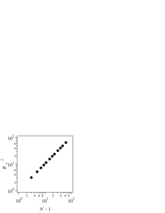
Figure 2: T. Uneyama and Y. Masubuchi to J. Chem. Phys

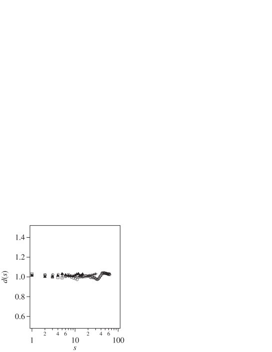
Figure 3: T. Uneyama and Y. Masubuchi to J. Chem. Phys

In this subsection static properties of the system is examined to show the consistency between simulation data and the equilibrium distribution function given by eq (8). Figure 2 shows the bond number $(N-1)$ dependence of squared end-to-end distance $R_{e}^{2}$ to report that the scaling obeys the Gaussian chain statistics. The internal chain structure is examined via the internal distance factor $d(s)$ defined as $d(s)=\langle(\bm{R}_{i,k+s}-\bm{R}_{i,k})^{2}\rangle/s$, and shown in Figure 3. $d(s)$ is reasonably close to unity independently of $s$ and $N$ as expected for the Gaussian chain statistics. These results demonstrate that the attractive force induced by the slip-springs is correctly compensated by the repulsive interaction. A similar attempt has been made for PCN model where the soft core repulsive interaction was introduced between slip-links[64], but a precise control of the chain dimension was difficult due to the lack of free energy expression for PCN model. (Indeed, it seems practically impossible to introduce the repulsive potential which exactly cancels the artificial attractive interaction in slip-link models such as the PCN model[53].)

Figure 4 shows the distribution of slip-spring number per chain $Z_{c}$, $P(Z_{c})$. The grand canonical type treatment of the slip-springs for single chain models predict the Poisson distribution for the number of slip-springs on a chain[54, 11]. Indeed, the results shown by symbols reasonably close to the Poisson distribution drawn by solid curves where the average value of $Z_{c}$ is given as $2,4,8$ and $16$ for the examined chains with $N=8,16,32$ and $64$, for the simulation parameter $N_{e}=4$ (calculated from the slip-spring density and the bead density as $N_{e}=2\phi\rho_{0}$).

3.2 Dynamics

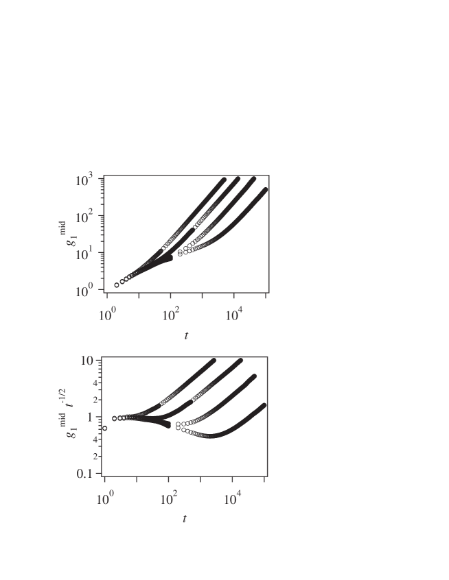
Figure 5: T. Uneyama and Y. Masubuchi to J. Chem. Phys

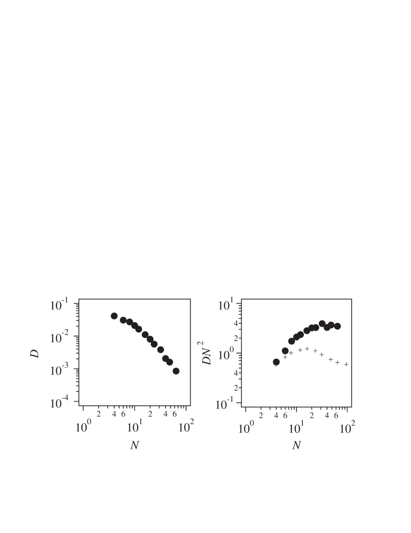
Figure 6: T. Uneyama and Y. Masubuchi to J. Chem. Phys

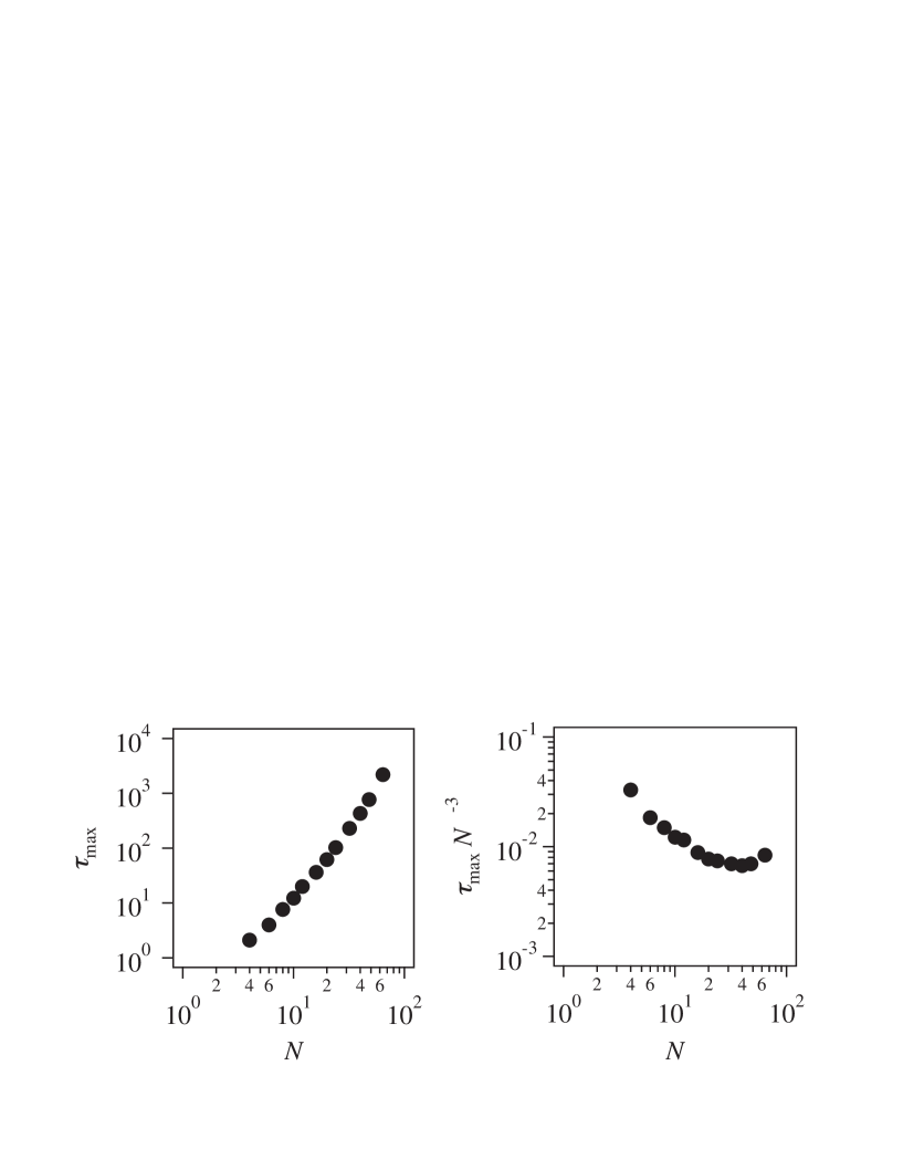
Figure 7: T. Uneyama and Y. Masubuchi to J. Chem. Phys

Figure 5 shows the mean square displacement of the central bead in the chain, $g_{1}^{\text{mid}}(t)$. To see the effect of the entanglement clearly, the data divided by the Rouse behavior in internal time range $g_{1}^{\text{mid}}(t)t^{-1/2}$ is also shown. From these plots, it is apparent that the entanglement effect appears after $t\sim 10$ where the negative slope starts in $g_{1}^{\text{mid}}(t)t^{-1/2}$. In this respect, the short chain with $N=8$ does not show the entangled behavior, in spite of the fact that there exist two slip-springs per chain on average as shown in Fig 4. Figure 6 shows the diffusion coefficient $D$ against the bead number $N$. To see the scaling behavior clearly, $DN^{2}$ is also shown. The Rouse behavior $D\propto N^{-1}$ is observed below $N=8$, which is consistent with what observed for $g_{1}^{\text{mid}}(t)$. For longer chains, the $N$ dependence is not that strong and actually the power law exponent does not largely deviate from $-2$ even for $N=64$, which is somewhat weaker than experimental results for well entangled systems[65]. In comparison with the literature data (shown by cross in the right panel) for single chain slip-spring model[10] with similar parameter setting (except the difference in $\zeta_{s}$ that is $1$ for our simulation while it is $0.1$ for the single chain data), it is suggested that the dynamical constraint in the present model is weaker than that in the single chain model. We expect that this is due to the difference in the hopping (sliding) kinetics of slip-springs. In our model the both ends of slip-springs are mobile while in the single chain models one end is anchored, as we mentioned in Section 2.6. This difference will result in a weaker constraint to the chain in our model. Indeed, similar behavior is observed in the $N$ dependence of the longest relaxation time for the end-to-end vector, $\tau_{\text{max}}$, shown in Fig 7. Especially, $\tau_{\text{max}}N^{-3}$ indicates that the large $N$ chains examined here are still in the transitional region between unentangled and entangled regimes.

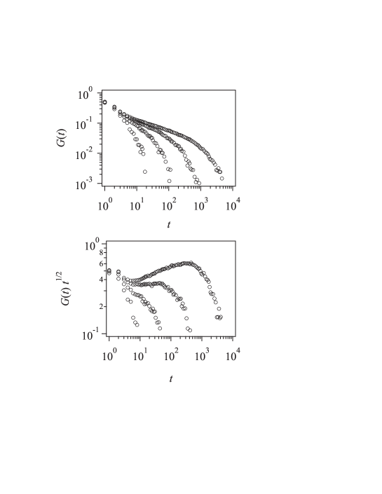
Figure 8: T. Uneyama and Y. Masubuchi to J. Chem. Phys

Figure 8 shows the relaxation modulus $G(t)$ calculated by the linear response theory shown in Sec. 2.4. Here, $G(t)$ is normalized by the unit modulus defined as $G_{0}\equiv\rho RT/M_{0}$[66]. As in the case of the mean square displacement, we also show the data divided by the Rouse behavior, $G(t)t^{1/2}$. As we have observed for $g_{1}^{\text{mid}}(t)$, the entanglement effect (the increase of $G(t)t^{1/2}$ in time) is not observed in short chains. On the other hand, for longer chains $G(t)$ apparently deviates from the Rouse relaxation to show the plateau, as expected. We note that the unit modulus $G_{0}$ is not equal to the plateau modulus $G_{N}$ and actually $G_{N}$ is much smaller than $G_{0}$. (This is because $G_{0}$ is a characteristic modulus for the bead scale, and it reflects the short time relaxation modes.) For the single chain model it is reported that $G_{N}\approx 0.1G_{0}$[10]. Our results for long chains are similar to this relation. Of course, the relation between $G_{N}$ and $G_{0}$ depends on the model and various parameters. The direct comparison of our result with the single chain simulation results seems to be difficult.

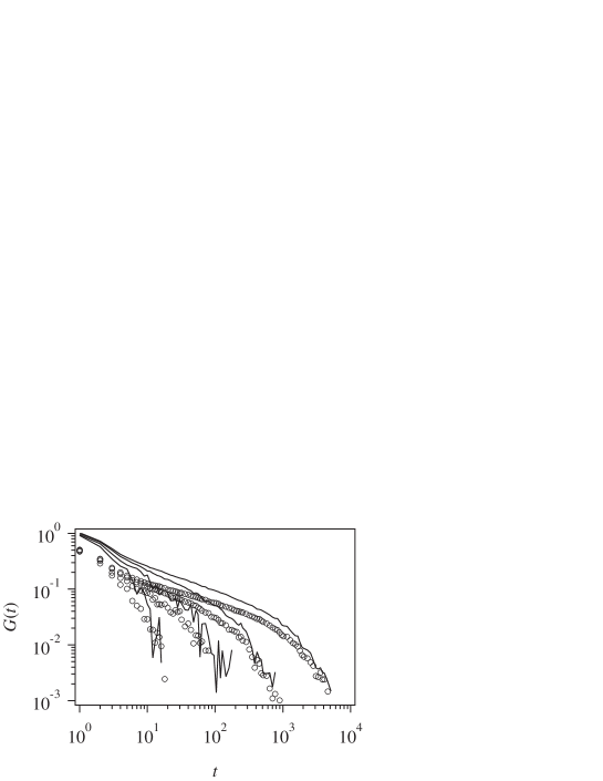
Figure 9: T. Uneyama and Y. Masubuchi to J. Chem. Phys

As we mentioned, there are two possible expressions for the stress tensor of the system. To investigate how the expression of the stress tensor affects the rheological properties, here we compare the shear relaxation moduli calculated with two different expressions. Figure 9 shows the shear relaxation moduli for $N=8,16,32$ and 64 calculated by eqs (38) (symbol) and (39) (solid curve). Although the shear relaxation moduli data by eqs (38) and (39) are quantitatively different, they are qualitatively similar, as reported in the single chain model.[11]

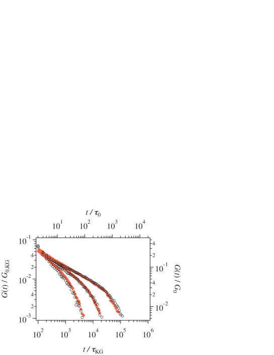
Figure 10: T. Uneyama and Y. Masubuchi to J. Chem. Phys

Figure 10 shows a comparison with the Kremer-Grest simulations[66] on $G(t)$. Here, $G(t)$ of our simulation is calculated by eq (38), but similar fitting can be realized for $G(t)$ obtained by eq (39) as well, if the parameters are adequately tuned (not shown here). There are small discrepancies in the short time region due to the difference in the level of coarse-graining, i.e., the number of Rouse modes. This discrepancy may be eliminated if $N_{e}$ value is increased as reported in the single chain model. For this fitting, we choose the parameters as follows.

$$M_{0}=3.1,\quad\tau_{0}=50\tau_{\text{KG}},\quad G_{0}=0.2G_{0,\text{KG}}$$ (52)

Here, $M_{0}$ is the number of beads (molecular weight) of the Kremer-Grest model which corresponds to one bead in our model, $\tau_{\text{KG}}$ is the unit time in the Kremer-Grest simulation (the standard time scale for particles with the Lennard-Jones potential), and $G_{0,\text{KG}}$ is the unit modulus for the Kremer-Grest model[66]. This fitting demonstrates that the dynamical constraint given by the slip-spring is relatively weak, and this result is consistent with results obtained by $D$ and $\tau_{\text{max}}$. For instance, it has been reported that the entanglement number for the Kremer-Grest chain with 200 beads is around 5[66]. On the other hand, the corresponding chain in our model is $N=64$ that has $16$ slip-springs per chain on average, as shown in Fig 4. Since the $G(t)$ data compared here are in the transitional regime and the contribution from the Rouse relaxation is relatively large, the fitting results (eq (52)) may be different for well-entangled systems. Nevertheless, the fact that $N_{e}$ is smaller than the effective entanglement bead number is informative. For this specific case, the effective entanglement bead number in our model is roughly estimated as $3N_{e}$. A similar result have been reported for the PCN model[37], and such a discrepancy is expected to be the nature of randomly connected multi chain network. From the similarity between our model and the PCN model, where the entanglements are not fixed in space, we consider the obtained results are reasonable.

In order to compare the computation cost (efficiency) of our model, we report CPU times for several different simulation models on a PC (Intel Xeon X5570 2.93GHz, Cent OS 4). We chose a melt of Kremer-Grest chains with bead number $N=200$ as a reference, and made calculations by the present model and by the PCN model for similar systems. Each simulation was performed for time steps comparable to the longest relaxation time. All the simulations were performed by serial simulation codes. The Kremer-Grest simulation was made by COGNAC ver 7.1.1[67]. The other simulations were performed by our home-made simulation codes. For a Kremer-Grest simulation with the chain number $M=6$, the required time steps is about $100,000$ and the CPU time was $60$ hours. For our model, a simulation with $N=64$, $M=32$, $N_{e}=4$ and $\zeta_{s}=1.0$, required the $3000$ time steps and the CPU time was $30$ minutes. For a PCN simulation with the average segment number of segments per chain $Z=15$ and the number of chains $M=341$ required $200$ time steps for the relaxation and the CPU time was $2$ minutes. From these results, we can conclude that the computational cost (efficiency) of our model is in between the Kremer-Grest model and the PCN model. Judging from the coarse-graining level of these models, this result is reasonable.

4 Conclusion

In this study, we proposed the multi-chain slip-spring model where the bead-spring chains are dispersed in space and connected by slip-springs. The entanglement effect is mimicked by the slip-springs and not by the hard-core (excluded volume) interaction between beads. Our model is located in the niche of the modeling of entangled polymer dynamics between conventional multi-chain simulations and single chain models. In our model, the set of state variables are the position of beads and the connectivity (bead indices) of the slip-springs. Differently from the primitive chain network model (that is the other class of multi-chain model), the total free energy of the system is well-defined, and kinetic equations are designed based on the free energy and the detailed balance condition. The free energy includes the repulsive interaction between beads, which compensate the attractive interaction artificially generated by the slip-springs. The explicit expression of linear relaxation modulus was also derived by the linear response theory. A possible numerical scheme was proposed and simulations reproduced expected bead number dependence in transitional regime between Rouse and entangled dynamics for the chain structure, the central bead diffusion and the linear relaxation modulus.

In this model there are a couple of parameters ($N_{s}$, $\zeta_{s}$, $\rho_{0}$ and $\phi$) of which effect on chain dynamics is not well understood. It would be an interesting work to explore the effects of these parameters by theoretical methods as well as simulations. We are performing simulations to scan these parameters and compare the resulting chain dynamics with the other models and experiments. Another interesting topic is on the extension of this model by using its multi-chain nature, as reported for PCN model, to branch polymers, blends and copolymers, etc. The results for these attempts will be reported elsewhere.

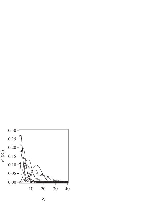
Figure 4: T. Uneyama and Y. Masubuchi to J. Chem. Phys

References

- [1] P. G. de Gennes, J. Chem. Phys. 55, 572 (1971).
- [2] M. Doi and S. F. Edwards, The Theory of Polymer Dynamics (Clarendon, Oxford, 1986).
- [3] H. Watanabe, Prog. Polym. Sci. 24, 1253 (1999).
- [4] T. C. B. McLeish, Adv. Phys. 51, 1379 (2002).
- [5] D.W. Mead, R.G. Larson and M. Doi, Macromolecules, 31, 7895 (1998).
- [6] C. C. Hua and J. D. Schieber, J. Chem. Phys. 109, 10018 (1998).
- [7] M. Doi and J.-I. Takimoto, Phil. Trans. R. Soc. Lond. A 361, 641 (2003).
- [8] A. E. Likhtman and T. C. B. McLeish, Macromolecules 35, 6332 (2002).
- [9] J. D. Schieber, J. Neergaard and S. Gupta, J. Rheol. 47, 213 (2003).
- [10] A. E. Likhtman, Macromolecules 38, 6128 (2005).
- [11] T. Uneyama, Nihon Reoroji Gakkaishi (J. Soc. Rheol. Jpn.) 39, 135 (2011).
- [12] M. Doi, J. Polym. Sci.: Polym. Lett. Ed. 19, 265 (1981).
- [13] S. T. Milner and T. C. B. McLeish, Phys. Rev. Lett. 81 725 (1998).
- [14] W. W. Graessley, Adv. Polym. Sci. 47, 67 (1982).
- [15] C. Tsenoglou, ACS Polym. Preprints 28, 185 (1987).
- [16] J. des Cloizeaux, Europhys. Lett. 5, 437 (1988).
- [17] G. Marrucci, J. Non-Newtonian Fluid Mech. 62, 279 (1996).
- [18] G. Ianniruberto and G. Marrucci, J. Non-Newtonian Fluid Mech. 65, 241 (1996).
- [19] K. Kremer and G. S. Grest, J. Chem. Phys. 92, 5057 (1990).
- [20] J. Ramos, J. F. Vega, D. N. Theodorou and J. Martinez-Salazar, Macromolecules 41, 2959 (2008).
- [21] C. Tzoumanekas and D. N. Theodorou, Curr. Opinion Solid State Mat. Sci. 10, 61 (2006).
- [22] A. Harmandaris and K. Kremer, Macromolecules 42, 791 (2009).
- [23] R. Everaers, S. K. Sukumaran, G. S. Grest, C. Svaneborg, A. Sivasubramanian, and K. Kremer, Science 303, 823 (2004).
- [24] M. Kröger, Comput. Phys. Commun. 168, 209 (2005).
- [25] K. Foteinopoulou, N. C. Karayiannis, V. G. Mavrantzas, and M. Kröger, Macromolecules 39, 4207 (2006).
- [26] C. Tzoumanekas and D. N. Theodorou, Macromolecules 39, 4592 (2006).
- [27] S. Shanbhag and R. G. Larson, Macromolecules 39, 2413 (2006).
- [28] J. Gao and J. H. Weiner, J. Chem. Phys. 98, 8256 (1993).
- [29] J. Cao and A. E. Likhtman, Phys. Rev. Lett. 104, 207801 (2010).
- [30] M. Kröger, C. Luap and R. Muller, Macromolecules 30, 526 (1997).
- [31] J. Ramírez, S. K. Sukumaran and A. E. Likhtman,J. Chem. Phys. 126, 244904 (2007).
- [32] Y. Masubuchi and S. K. Sukumaran, Nihon Reoroji Gakkaishi (J. Soc. Rheol. Jpn.), in print.
- [33] J. T. Padding and W. J. Briels, J. Chem. Phys. 115, 2846 (2001).
- [34] Y. Masubuchi, J.-I. Takimoto, K. Koyama, G. Ianniruberto, G. Marrucci and F. Greco, J. Chem. Phys. 115, 4387 (2001).
- [35] P. Kindt and W. J. Briels, J. Chem. Phys. 127, 134901 (2007).
- [36] J. T. Padding and W.J. Briels, J. Phys.: Condens. Matter 23, 233101 (2011).
- [37] Y. Masubuchi, G. Ianniruberto, F. Greco and G. Marrucci, J. Chem. Phys. 119, 6925 (2003).
- [38] Y. Masubuchi, G. Ianniruberto, F. Greco and G. Marrucci, Modelling Simulation Mat. Sci. Eng. 12, S91 (2004).
- [39] Y. Masubuchi, G. Ianniruberto, F. Greco, G. Marrucci, J. Non-Newtonian Fluid Mech. 149, 87 (2008).
- [40] Y. Masubuchi, Y. Matsumiya and H. Watanabe, J. Chem. Phys. 134, 194905 (2011).
- [41] Y. Masubuchi, Y. Matsumiya, H. Watanabe, S. Shiromoto, M. Tsutsubuchi and Y. Togawa, Rheol. Acta 51, 193 (2012).
- [42] Y. Masubuchi, G. Ianniruberto, F. Greco and G. Marrucci, J. Non-Crystal. Solids, 352, 5001 (2006).
- [43] K. Furuichi, C. Nonomura, Y. Masubuchi, H. Watanabe, G. Ianniruberto, F. Greco and G. Marrucci, Rheol. Acta 47, 591 (2008).
- [44] Y. Masubuchi, K. Furuichi, K. Horio, T. Uneyama, H. Watanabe, G. Ianniruberto, F. Greco and G. Marrucci, J. Chem. Phys. 131, 114906 (2009).
- [45] A. Dambal, A. Kushwaha and E. Shaqfeh, Macromolecules 42, 7168 (2009).
- [46] K. Furuichi, C. Nonomura, Y. Masubuchi and H. Watanabe, J. Chem. Phys. 133, 174902 (2010).
- [47] A. Kushwaha and E. Shaqfeh, J. Rheol. 55, 463 (2011).
- [48] T. Yaoita, T. Isaki, Y. Masubuchi, H. Watanabe, G. Ianniruberto and G. Marrucci, Macromolecules 44, 9675 (2011).
- [49] T. Yaoita, T. Isaki, Y. Masubuchi, H. Watanabe, G. Ianniruberto and G. Marrucci, Macromolecules 45, 2773 (2012).
- [50] Y. Masubuchi, H. Watanabe, G. Ianniruberto, F. Greco and G. Marrucci, Macromolecules 41, 8275 (2008).
- [51] Y. Masubuchi, T. Uneyama, H. Watanabe, G. Ianniruberto, F. Greco, and G. Marrucci, J. Chem. Phys. 132, 134902 (2010).
- [52] T. Uneyama and Y. Masubuchi, J. Chem. Phys. 135, 184904 (2011).
- [53] T. Uneyama and K. Horio, J. Polym. Sci. B: Polym. Phys. 49, 966 (2011).
- [54] J. D. Schieber, J. Chem. Phys. 118, 5162 (2003).
- [55] P. J. Flory and W. R. Krigbaum, J. Chem. Phys. 18, 1086 (1950).
- [56] R. J. Glauber, J. Math. Phys. 4, 294 (1963).
- [57] H. Risken, The Fokker-Planck Equation, 2nd ed. (Springer, Berlin, 1989).
- [58] J. Gao and J. H. Weiner, J. Chem. Phys. 103, 1621 (1995).
- [59] R. Yamamoto and A. Onuki, Phys. Rev. E 70, 041801 (2004).
- [60] D. M. Nair and J. D. Schieber, Macromolecules 39, 3386 (2006).
- [61] R. Khaliullin and J. D. Schieber, Macromolecules 42, 7504 (2009).
- [62] E. Pilyugina, M. Andreev and J. D. Schieber, Macromolecules 45, 5728 (2012).
- [63] R. Khaliullin and J. D. Schieber, Macromolecules 43, 6202 (2010).
- [64] S. Okuda, T. Uneyama, Y. Inoue, Y. Masubuchi and M. Hojo, Nihon Reoroji Gakkaishi (J. Soc. Rheol. Jpn.) 40, 21 (2011).
- [65] T. P. Lodge, Phys. Rev. Lett. 83, 3218 (1999).
- [66] A. Likhtman, S. K. Sukumaran and J. Ramirez, Macromolecules 40, 6748 (2007).
- [67] http://octa.jp