A backward $\lambda$-Lemma for the forward heat flow

Abstract

The inclination or $\lambda$-Lemma is a fundamental tool in finite dimensional hyperbolic dynamics. In contrast to finite dimension, we consider the forward semi-flow on the loop space of a closed Riemannian manifold $M$ provided by the heat flow. The main result is a backward $\lambda$-Lemma for the heat flow near a hyperbolic fixed point $x$. There are the following novelties. Firstly, infinite versus finite dimension. Secondly, semi-flow versus flow. Thirdly, suitable adaption provides a new proof in the finite dimensional case. Fourthly and a priori most surprisingly, our $\lambda$-Lemma moves the given disk transversal to the unstable manifold backward in time, although there is no backward flow. As a first application we propose a new method to calculate the Conley homotopy index of $x$.

1 Introduction and main results

Assume $M$ is a closed smooth manifold of dimension $n\geq 1$ equipped with a Riemannian metric $g$ and the Levi-Civita connection $\nabla$. Throughout smooth means $C^{\infty}$ smooth. The loop space is the Hilbert manifold $\Lambda M:=W^{1,2}(S^{1},M)$ of absolutely continuous loops in $M$ with square integrable derivative. We identify $S^{1}={\mathbb{R}}/{\mathbb{Z}}$ and think of $\gamma\in\Lambda M$ as a map $\gamma:{\mathbb{R}}\to M$ that satisfies $\gamma(t+1)=\gamma(t)$. Pick a smooth function $V:S^{1}\times M\to{\mathbb{R}}$ and set $V_{t}(q):=V(t,q)$.

Consider the heat equation

$${\partial}_{s}u-\nabla\kern-2.15277pt{}_{t}{\partial}_{t}u-{\rm grad}V_{t}(u)=0$$ (1)

for smooth maps ${\mathbb{R}}\times S^{1}\to M:(s,t)\mapsto u(s,t)$. It is well known that the corresponding Cauchy problem for the map $[0,\infty)\to\Lambda M:s\mapsto u_{s}:=u(s,\cdot)$ admits a unique solution. The associated forward semi-flow $\varphi$ on $\Lambda M$ is called the heat flow. It is a continuous map

$$\varphi:[0,\infty)\times\Lambda M\to\Lambda M$$

which is of class $C^{1}$ on $(0,\infty)$; see (5) for its representative $\phi$ in local coordinates. For $\gamma\in\Lambda M$ abbreviate $\dot{\gamma}=\frac{d}{dt}\gamma$. Because (1) is the downward $L^{2}$ gradient equation of the action functional ${\mathcal{S}}_{V}:\Lambda M\to{\mathbb{R}}$ given by

$${\mathcal{S}}_{V}(\gamma)=\int_{0}^{1}\left(\frac{1}{2}\mathopen{|}\dot{\gamma}(t)\mathclose{|}^{2}-V_{t}(\gamma(t))\right)dt,$$

the fixed points of the heat flow are the critical points of the action. The latter are (perturbed) closed geodesics, that is solutions $x:S^{1}\to M$ to the second order ODE

$$-\nabla\kern-2.15277pt{}_{t}\dot{x}-\nabla V_{t}(x)=0.$$

By ${\rm ind}(x)$ we denote the Morse index of $x$. Nondegeneracy of the critical point $x$, that is nondegeneracy of the Hessian of ${\mathcal{S}}_{V}$ at $x$, corresponds to hyperbolicity of the fixed point $x$.

Fix a nondegenerate critical point $x$ of the action ${\mathcal{S}}_{V}$. While the stable manifold $W^{s}(x)$ is defined in the usual way as the set of all points which flow in forward time asymptotically into $x$, it is of infinite dimension. The fact that $W^{s}(x)$ is globally embedded is, firstly, remarkable since the standard method of pulling back coordinates near $x$ using the backward flow is obviously not available. Secondly, except for (Henry-81-GeomTheory, , Thm. 6.1.9) this fact is usually not mentioned at all in the literature—unlike the widely known local submanifold property near $x$; see Section 2.5. In contrast, without a backward flow the definition of the unstable manifold $W^{u}(x)$ becomes somewhat awkward: It is the set of endpoints of all heat flow trajectories parametrized by $(-\infty,0]$ and emanating at time $-\infty$ from $x$. On the other hand, this definition lends itself to define a backward flow on $W^{u}(x)$ which immediately implies that the unstable manifold is globally embedded. Most importantly, its dimension given by ${\rm ind}(x)$ is finite; see e.g. Joa-HEATMORSE-II . It is this finite dimensionality which is one of two pillars on which this paper is based. A key consequence is smoothness of every $\gamma\in W^{u}(x)$; see Remark 3.

1.1 Some history

In finite dimensional hyperbolic dynamics there are two fundamental tools: The Grobman-Hartman Theorem Grobman-59 ; Hartman-60 and the $\lambda$-Lemma Palis-MS . While the first is powerful concerning topological questions the latter reigns in the differentiable world. It even implies the former. The $\lambda$-Lemma asserts that the backward flow applied to any disk ${\mathcal{D}}$ transversal to the unstable manifold and of complementary dimension converges in $C^{1}$ to the local stable manifold, see Figure 1, and similarly for the forward flow. For a beautiful presentation see Palis-deMelo . Since convergence is in $C^{1}$, the $\lambda$-Lemma is also called inclination lemma.

The second pillar on which this paper is based is the replacement of the absent backward flow on the loop space by the family of preimages $s\mapsto{\varphi_{s}}^{-1}{\mathcal{D}}$. This idea was born when we attempted to construct a Morse filtration of the loop space using the method of Abbondandolo and Majer AM-LecsMCInfDimMfs . Their construction builds on open sets being mapped to open sets under a forward flow. But this is not true for $\varphi_{s}$—from a topological point of view the heat semi-flow is useless! The way out was the simple observation that preimages of open sets are open by continuity of $\varphi_{s}$. Unfortunately, still the Abbondandolo-Majer method would not apply, because things were moving in the wrong direction now. However, the definition given in (Dietmar-BLMS, , proof of Lemma 3.2) in finite dimensions carries over providing a Conley pair $(N,L)$ for the semi-flow invariant set given by the critical point $x$. Now the backward $\lambda$-Lemma enters. In Joa-JOAOPESSOA ; Joa-CONLEY we use it to define an invariant stable foliation of $(N,L)$ which is a fundamental ingredient in our construction of a Morse filtration of $\Lambda M$ by open semi-flow invariant sets. In Section 1.4 we discuss the key calculation.
In other words, we were led to discover the backward $\lambda$-Lemma through the attempt to solve a very different problem—thereby reconfirming a major principle advocated by V.I. Arnol’d throughout his mathematical life.

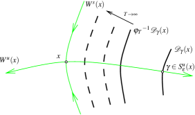
Figure 1: Preimage of disk ${\mathcal{D}}_{\gamma}(x)$ converges in $C^{1}$ and locally near $x$ to the stable manifold $W^{s}(x)$

1.2 Main results

Assume ${\mathcal{D}}_{\gamma}(x)$ is a disk in the Hilbert manifold $\Lambda M=W^{1,2}(S^{1},M)$ which intersects the unstable manifold $W^{u}(x)$ transversally in a point $\gamma$ near $x$. Our main goal is to prove that the preimage ${\varphi_{T}}^{-1}{\mathcal{D}}_{\gamma}(x)$ converges, as $T\to\infty$, uniformly in $C^{1}$ and locally near $x$ to the stable manifold $W^{s}(x)$; see Figure 1. In fact, we prove right away a family version where ${\mathcal{D}}$ is fibered over a descending sphere $S^{u}_{\varepsilon}(x)=W^{u}(x)\cap\{{\mathcal{S}}_{V}={\mathcal{S}}_{V}(x)-{\varepsilon}\}$.

Since the $\lambda$-Lemma is a local result we choose a local parametrization

$$\Phi:=\exp_{x}:X\to\Lambda M,\qquad X=T_{x}\Lambda M=W^{1,2}(S^{1},x^{*}TM),$$

of an open neighborhood of $x$ in $\Lambda M$ in terms of the exponential map; here compactness of $M$ enters. The orthogonal splitting

$$X\simeq T_{x}W^{u}(x)\oplus T_{x}W^{s}(x)=X^{-}\oplus X^{+}$$

with associated orthogonal projections $\pi_{\pm}$ is a key ingredient to make the analysis work; at this stage take the final identity as a definition. By a standard graph argument we may assume without loss of generality that ${\mathcal{U}}$ is of the form $W^{u}\times{\mathcal{O}}^{+}$. Here $W^{u}\subset X^{-}$ represents a descending disk $W^{u}(x)\cap\{{\mathcal{S}}_{\mathcal{V}}>{\mathcal{S}}_{\mathcal{V}}(x)-\delta\}$ for some $\delta>0$ sufficiently small and ${\mathcal{O}}^{+}\subset X^{+}$ is an open ball about $0$. By $\phi$ we denote the local semi-flow on ${\mathcal{U}}$ which represents the heat flow $\varphi$ on $\Lambda M$ with respect to the local parametrization $\Phi$; see (5).

Hypothesis 1 (Local setup—Figure 4)

Fix a perturbation $V\in C^{\infty}(S^{1}\times M)$ and a nondegenerate critical point $x$ of ${\mathcal{S}}_{V}$ of Morse index $k$.
(a) Consider the coordinates on $\Lambda M$ provided by $\Phi$ and modelled on the open subset ${\mathcal{U}}=W^{u}\times{\mathcal{O}}^{+}$ of $X$. In these coordinates the origin $0\in X$ represents $x$ and ${\mathcal{S}}:={\mathcal{S}}_{V}\circ\Phi^{-1}$ represents the action. We denote closed radius $R$ balls about $0$ by

$${\mathcal{B}}_{R}:=\{\left\|\cdot\right\|_{X}\leq R\},\qquad{\mathcal{B}}^{+}_{R}:=\{\left\|\cdot\right\|_{X^{+}}\leq R\}.$$

Choose the constant $\rho_{0}>0$ in the Lipschitz Lemma 1 smaller, if necessary, such that ${\mathcal{B}}_{\rho_{0}}\subset{\mathcal{U}}$. Pick a sufficiently small constant ${\varepsilon}_{0}>0$ such that for each ${\varepsilon}\in(0,{\varepsilon}_{0}]$ the descending and ascending disks

$$W^{u}_{\varepsilon}(x):=W^{u}(x)\cap\{{\mathcal{S}}_{V}>{\mathcal{S}}_{V}(x)-{\varepsilon}\},\quad W^{s}_{\varepsilon}(x):=W^{s}(x)\cap\{{\mathcal{S}}_{V}<{\mathcal{S}}_{V}(x)+{\varepsilon}\},$$

are contained in the coordinate patch $\Phi({\mathcal{B}}_{\rho_{0}})$ and such that their closures are diffeomorphic to the closed unit disks in ${\mathbb{R}}^{k}$ and $X^{+}$, respectively. Existence of ${\varepsilon}_{0}$ follows by the Morse- and the Palais-Morse lemma.
(b) Fix $\mu\in(0,d)$ in the spectral gap (4) of the Jacobi operator. Pick $\varkappa\in(0,\rho_{0})$ so small that ${\mathcal{D}}:=S^{u}_{\varepsilon}\times{\mathcal{B}}^{+}_{\varkappa}$ is contained in ${\mathcal{B}}_{\rho_{0}}$ and set ${\mathcal{D}}_{\gamma}:=\{\gamma\}\times{\mathcal{B}}^{+}_{\varkappa}$.
(c) Our notation for objects expressed in coordinates will be the global notation with $x$ omitted, for example $W^{s}_{\varepsilon}$ and ${\mathcal{D}}_{\gamma}$.

Theorem 1.1 (Backward $\lambda$-Lemma)

Assume the local setup of Hypothesis 1. In particular, consider the hyperbolic fixed point $0$ of the local semi-flow $\phi$ defined by (5) on ${\mathcal{U}}\subset X$ and the hypersurface ${\mathcal{D}}=S^{u}_{\varepsilon}\times{\mathcal{B}}^{+}_{\varkappa}\subset{\mathcal{B}}_{\rho_{0}}\subset{\mathcal{U}}$; see Figure 2. Then the following is true. There is a closed ball ${\mathcal{B}}^{+}\subset X^{+}$ of radius $r>0$ about zero, a constant $T_{0}>0$, and a Lipschitz continuous map

$$\begin{split}{\mathcal{G}}:(T_{0},\infty)\times S^{u}_{\varepsilon}\times{\mathcal{B}}^{+}&\to W^{u}\times{\mathcal{B}}^{+}\subset{\mathcal{U}}\\ (T,\gamma,z_{+})&\mapsto\left(G^{T}_{\gamma}(z_{+}),z_{+}\right)=:{\mathcal{G}}^{T}_{\gamma}(z_{+})\end{split}$$

of class $C^{1}$ and defined by (25). Each map ${\mathcal{G}}^{T}_{\gamma}:{\mathcal{B}}^{+}\to X$ is bi-Lipschitz, a diffeomorphism onto its image, and ${\mathcal{G}}^{T}_{\gamma}(0)=\phi_{-T}\gamma=:\gamma_{T}$. The graph of $G^{T}_{\gamma}$ consists of those $z\in{\mathcal{U}}$ which satisfy $\pi_{+}z\in{\mathcal{B}}^{+}$ and reach the fiber ${\mathcal{D}}_{\gamma}=\{\gamma\}\times{\mathcal{B}}^{+}_{\varkappa}$ at time $T$, that is

$${\mathcal{G}}^{T}_{\gamma}({\mathcal{B}}^{+})={\phi_{T}}^{-1}{\mathcal{D}}_{\gamma}\cap\left(X^{-}\times{\mathcal{B}}^{+}\right).$$

Furthermore, the graph map ${\mathcal{G}}^{T}_{\gamma}$ converges uniformly, as $T\to\infty$, to the stable manifold graph map ${\mathcal{G}}^{\infty}$ of Theorem 2.1. More precisely, it holds that 

$$\begin{split}\left\|{\mathcal{G}}^{T}_{\gamma}(z_{+})-{\mathcal{G}}^{\infty}(z_{+})\right\|_{C^{1}(S^{1})}\leq\rho_{0}e^{-T\frac{\mu}{16}}\end{split}$$

for all $T>T_{0}$, $\gamma\in S^{u}_{\varepsilon}$, and $z_{+}\in{\mathcal{B}}^{+}$.

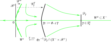
Figure 2: Backward $\lambda$-Lemma

Theorem 1.2 (Uniform $C^{1}$ convergence on $X$)

Under the assumptions of Theorem 1.1 the linearized graph maps $d{\mathcal{G}}^{T}_{\gamma}(z_{+}):X^{+}\to X$ extend to bounded linear operators on the $L^{2}$ completions and their limit, as $T\to\infty$, is $d{\mathcal{G}}^{\infty}(z_{+})$, uniformly in $z_{+}\in{\mathcal{B}}^{+}$. More precisely,

$$\left\|d{\mathcal{G}}^{T}_{\gamma}(z_{+})v\right\|_{2}\leq 2\left\|v\right\|_{2}$$

and

$$\left\|d{\mathcal{G}}^{T}_{\gamma}(z_{+})v-d{\mathcal{G}}^{\infty}(z_{+})v\right\|_{2}\leq e^{-T\frac{\mu}{16}}\left\|v\right\|_{2}$$

for all $T>T_{0}$, $\gamma\in S^{u}_{\varepsilon}$, $z_{+}\in{\mathcal{B}}^{+}$, and $v$ in the $L^{2}$ closure of $X^{+}$.

Remark 1

(i) The reason why the $W^{1,2}$ norm has been replaced by $C^{1}$ ($\hookleftarrow W^{1,4}$) in Theorem 1.1 and by $L^{2}$ in Theorem 1.2 is the application in Section 1.4. Here the $L^{2}$ nature of (1) requires to estimate the nonlinearity $f$ in (5) in the $L^{2}$ norm. But $f$ maps $W^{1,4}$ to $L^{2}$.

(ii) All results in this paper extend to the more general class of perturbations satisfying axioms (V0-V3) in SaJoa-LOOP ; see Joa-LOOPSPACE .

Remark 2

(a) Theorem 1.1 recovers the common case of a single disk intersecting the unstable manifold transversely in one point $\gamma$ near $0$. Apply the implicit function theorem to bring the disk into the normal form $\{\gamma\}\times{\mathcal{B}}^{+}_{\varkappa}$. Observe that ${\mathcal{G}}^{T}_{\gamma}$ is defined without reference to any neighbors of $\gamma$. To formally get a bundle ${\mathcal{D}}=S^{u}_{\varepsilon}\times{\mathcal{B}}^{+}_{\varkappa}$ as in the hypothesis just add disks artificially.
(b) Theorem 1.1 for endpoint time $T=\infty$ and radius $\varkappa=0$ recovers two known results. These appear as extreme cases concerning the radius $0$ disk bundle ${\mathcal{D}}=S^{u}_{\varepsilon}\times\{0\}$.

1. Disk of radius $0$ sitting at the origin: In this case $S^{u}_{\varepsilon}=\{0\}$, that is the disk bundle degenerates to just one radius $0$ disk sitting at the origin. This recovers the local stable manifold Theorem 2.1 and inspires the notation ${\mathcal{G}}^{\infty}$ for the stable manifold graph map. The preimage ${\phi_{T}}^{-1}(0)$ for $T=\infty$ corresponds to the local stable manifold.

2. Radius $0$ disk bundle sitting at $\infty$: This recovers the stable foliation in CHOW-LIN-LU . Two points belong to the same leaf if under the semi-flow $\phi_{s}$ their difference converges exponentially to zero, as $s\to\infty$. The leaf over $0$ is the local stable manifold.

Remark 3 (Mixed Cauchy problem)

We motivate why the map ${\mathcal{G}}$ in the backward $\lambda$-Lemma should exist. Assume the hypotheses of the backward $\lambda$-Lemma and fix $T>0$. Each point $z$ in the preimage ${\phi_{T}}^{-1}{\mathcal{D}}_{\gamma}$ corresponds to a unique semi-flow line $\xi$ such that $\xi(0)=z$ and $\xi$ hits the fiber ${\mathcal{D}}_{\gamma}$ precisely at time $T$, say in the point $q:=\xi(T)$. Of course, we cannot change the order, i.e. first choosing an end point $q\in{\mathcal{D}}_{\gamma}$ and then determining a semi-flow line $\xi$ with $\xi(T)=q$. This would amount to solve the Cauchy problem for the heat equation in backward time, a problem well known to be ill defined in general: Indeed any non-smooth element $q\in{\mathcal{D}}_{\gamma}\subset W^{1,2}$ cannot be reached, since the point $\xi(T)$ on any heat flow trajectory $\xi$ is necessarily a smooth loop in $M$—due to the strongly regularizing effect of the heat flow for $T>0$; see e.g. Joa-LOOPSPACE . However, consider the splitting $X=X^{-}\oplus X^{+}$ in unstable and stable tangent spaces. In Section 2.3 we will see that each element of $X^{-}$ is smooth. So specifying only the $X^{-}$ part of the endpoint does not contradict regularity to start with. The key idea is to introduce the notion of a mixed Cauchy problem: Apart from time $T$ only the stable part $z_{+}$ of the initial point is prescribed—in exchange of prescribing in addition the unstable part $q_{u}$ of the end point; see Figure 3. Indeed the representation formula in Proposition 2 shows that the mixed Cauchy problem is equivalent to the usual Cauchy problem with initial value $z$. Since the latter admits a unique solution, so does the mixed Cauchy problem.

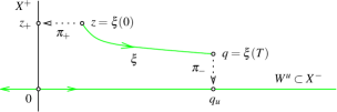
Figure 3: Data $(T,q_{u},z_{+})$ for mixed Cauchy problem

1.3 Outlook

To put the backward $\lambda$-Lemma and the associated stable foliations Joa-CONLEY in perspective recall the celebrated proof by Palis in his 1967 PhD thesis Palis-PhD of Andronov-Pontryagin structural stability of hyperbolic dynamical systems in small dimensions. Key innovations and tools in his proof were the notions of stable and unstable foliations which led to numerous applications ever since.

Another interesting perspective of the backward $\lambda$-Lemma is that, to the best of our knowledge, it provides the first backward time information concerning the heat flow—apart from the obvious backward flow on the (finite dimensional) unstable manifolds. In fact the backward $\lambda$-Lemma provides backward time information on open subsets.

Going from (1) and $W^{1,2}$ to general semilinear parabolic PDEs and $W^{k,p}$ will be investigated elsewhere.

1.4 Application

The method in Joa-JOAOPESSOA ; Joa-CONLEY to construct a Morse filtration of the loop space is inspired by Conley theory CONLEY-CBMS . For reals ${\varepsilon},\tau>0$ denote by $N$ the path connected component of $x$ of the open set $\{\gamma\in\Lambda M\mid\text{${\mathcal{S}}_{V}(\gamma)<{\mathcal{S}}_{V}(x)+{\varepsilon}$, ${\mathcal{S}}_{V}(\varphi_{\tau}\gamma)>{\mathcal{S}}_{V}(x)-{\varepsilon}$}\}$. For ${\varepsilon}>0$ small and $\tau>0$ large the closed subset $L:=\{\gamma\in N\mid\text{${\mathcal{S}}_{V}(\varphi_{2\tau}\gamma)\leq{\mathcal{S}}_{V}(x)-{\varepsilon}$}\}$ of $N$ is an exit set of $N$ and $(N,L)$ is a Conley pair for the semi-flow invariant set $\{x\}$; see Joa-CONLEY ; Joa-LOOPSPACE . Concerning the Morse filtration a fundamental step is to prove that relative singular homology is given by

$${\rm H}_{\ell}(N,L)\simeq\begin{cases}{\mathbb{Z}}&,\ell=k:={\rm ind}(x),\\ 0&\text{, otherwise.}\end{cases}$$

Because the part of $N$ in the unstable manifold is an open $k$ disk bounded by the (relatively) closed annulus $L\cap W^{u}(x)$, the relative homology of these parts has the required property and it suffices to show that $(N\cap W^{u}(x),L\cap W^{u}(x))$ is a deformation retract of $(N,L)$. Observe that $N$ contains the ascending disk $W^{s}_{\varepsilon}(x)$—from now on abbreviated $W^{s}_{\varepsilon}$—whose part in the unstable manifold is precisely the critical point $x$ itself. Thus on $W^{s}_{\varepsilon}$ the semi-flow $\varphi_{s}$ itself provides the desired deformation. Obviously this fails on the complement of the ascending disk. Now the backward $\lambda$-Lemma comes in. It naturally endows $(N,L)$, as we show in Joa-CONLEY , with the structure of a codimension $k$ foliation whose leaves $N(\gamma_{u})$ are parametrized by $\gamma_{u}\in N\cap W^{u}(x)$. Furthermore, each leaf is diffeomorphic to a neighborhood $U_{\gamma_{u}}$ of $W^{s}_{\varepsilon}$ in $W^{s}(x)$. The leaf through $x$ is given by $N(x)=W^{s}_{\varepsilon}=U_{x}(W^{s}_{\varepsilon})$. These diffeomorphisms, denoted by

$$\Psi_{\gamma_{u}}:U_{\gamma_{u}}(W^{s}_{\varepsilon})\stackrel{{\scriptstyle\simeq\,\,}}{{\longrightarrow}}N(\gamma_{u}),\qquad\Psi_{\gamma_{u}}(x)=\gamma_{u},\qquad\Psi_{0}=id_{W^{s}_{\varepsilon}},$$

allow to extend to all of $N$ the desirable deformation property provided by $\varphi_{s}$ on $W^{s}_{\varepsilon}$. Indeed pick $\gamma\in N$. By the foliation property $\gamma$ lies on some leaf, say on $N(\gamma_{u})$. Now the map $\theta_{s}(\gamma):=\Psi_{\gamma_{u}}\circ\varphi_{s}\circ{\Psi_{\gamma_{u}}}^{-1}(\gamma)$ for $s\in[0,\infty]$ deforms $N$ onto its part in the unstable manifold. So we are done. Well, note the subtlety arising due to the deformation having to take place entirely in $N$ which is equivalent to invariance of $U_{\gamma_{u}}(W^{s}_{\varepsilon})$ under $\varphi_{s}$. For $U_{x}(W^{s}_{\varepsilon})=W^{s}_{\varepsilon}$ this follows immediately from the fact that the action decreases along the heat flow. Since $\dim U_{\gamma_{u}}(W^{s}_{\varepsilon})=\infty$, the general case is non-trivial. Apart from the Palais-Smale condition, the analytic properties of the graph maps ${\mathcal{G}}^{T}_{\gamma}$ provided by Theorems 1.1 and 1.2 enter heavily. We refer to Joa-CONLEY for details and to Joa-JOAOPESSOA for a survey.

2 Toolbox

Throughout we fix a nondegenerate critical point $x$ of ${\mathcal{S}}_{V}:\Lambda M\to{\mathbb{R}}$. Representing the Hessian of ${\mathcal{S}}_{V}$ at $x$ with respect to the $L^{2}$ inner product on the loop space gives rise to the Jacobi operator $A_{x}$ defined by

$$A_{x}\xi=-\nabla\kern-2.15277pt{}_{t}\nabla\kern-2.15277pt{}_{t}\xi-R(\xi,\dot{x})\dot{x}-\nabla\kern-2.15277pt{}_{\xi}\nabla V_{t}(x)$$ (2)

for every smooth vector field $\xi$ along the loop $x$. Here $R$ denotes the Riemannian curvature tensor. Viewed as unbounded operator on a general Sobolev space $W^{k,q}:=W^{k,q}(S^{1},x^{*}TM)$ with dense domain $W^{k+2,q}$, where $k\in{\mathbb{N}}_{0}$ and $q\geq 1$, the spectrum of $A_{x}$ does not depend on $(k,q)$ and takes the form of a sequence of real eigenvalues (counting multiplicities)

$$\lambda_{1}\leq\lambda_{2}\leq\ldots\leq\lambda_{k}<0<\lambda_{k+1}\leq\lambda_{k+2}\leq\ldots$$ (3)

which converges to $\infty$. Calculation of the spectrum is standard: One picks the Hilbert space case $(k,q)=(0,2)$ and proves first that $A_{x}$ admits a compact self-adjoint resolvent. In the second step it remains to prove $C^{\infty}$ regularity of eigenfunctions. The spectral gap $(0,d)$ of $A_{x}$ is determined by

$$d:=dist\left(0,\sigma(A)\right)=\min\{-\lambda_{k},\lambda_{k+1}\}>0.$$ (4)

By $\sigma_{\pm}$ we denote the positive and negative part of the spectrum of $A_{x}$. Note that nondegeneracy of the critical point $x$ means that zero is not in the spectrum of $A_{x}$. Equivalently $x$ is a hyperbolic fixed point of $\varphi_{s}$ whenever $s>0$, that is the spectrum of the linearized flow $d\varphi_{s}(x)$ does not contain $1$. The Morse index of $x$ is the number $k$ of negative eigenvalues of $A_{x}$ counted with multiplicities.

It is worthwhile to mention some of the useful properties enjoyed by the action functional: It strictly decreases along non-constant heat flow trajectories. It is bounded below and satisfies the Palais-Smale condition.

In the following subsections we provide the analytical tools required in the proof of the backward $\lambda$-Lemma. Apart from Lemma 1 they are all well known, surely by the experts, and so we simply list them without proofs. On the other hand, some are difficult to find in the literature, e.g. sectoriality of $A_{x}$ in the relevant periodic case. So here is some good news for non-experts:

Convention. The proof of any assertion attributed well known in Section 2 is given in Joa-LOOPSPACE . The same holds for facts stated without reference.

2.1 Local semi-flow

Recall that ${\mathcal{U}}=W^{u}\times{\mathcal{O}}^{+}$ by Hypothesis 1. Any path $[0,T]\ni s\mapsto u_{s}$ in the neighborhood ${\mathcal{U}}(x):=\Phi({\mathcal{U}})$ of $x$ in the Hilbert manifold $\Lambda M$ corresponds to a path $\zeta:[0,T]\to{\mathcal{U}}$, $s\mapsto\zeta(s)$, determined uniquely by the identity $u_{s}=\exp_{x}\zeta(s)=:\Phi(\zeta(s))$ pointwise for $t\in S^{1}$. Applying the operators ${\partial}_{s}$ and $\nabla\kern-2.15277pt{}_{t}\nabla\kern-2.15277pt{}_{t}$ to this identity transforms the Cauchy problem on $\Lambda M$ associated to (1) into the equivalent Cauchy problem

$$\frac{d}{ds}\zeta(s)+A_{x}\zeta(s)=f(\zeta(s)),\qquad\zeta(0)=z:=\Phi^{-1}(\gamma)\in{\mathcal{U}},$$ (5)

for maps $\zeta:[0,T]\to{\mathcal{U}}\subset X=W^{1,2}(S^{1},x^{*}TM)$ where $T$ depends on $z\in{\mathcal{U}}$ and $A_{x}$ denotes the Jacobi operator (2) on $W^{1,2}$ with dense domain $W^{3,2}$. The solution to (5) defines the local semi-flow $\phi_{s}z:=\zeta(s)$ on ${\mathcal{U}}$ that represents the heat flow. The nonlinearity

$$f:X\supset{\mathcal{U}}\to Y,\qquad X=W^{1,2},\qquad Y=L^{1},$$

actually maps $W^{1,2p}$ to $L^{p}$ for $p\geq 1$ and is given by the identity

$$\begin{split}f(\zeta)&=E_{2}(x,\zeta)^{-1}\Bigl{(}E_{11}(x,\zeta)\bigl{(}\dot{x},\dot{x}\bigr{)}+2E_{12}(x,\zeta)\bigl{(}\dot{x},\nabla\kern-2.15277pt{}_{t}\zeta\bigr{)}\\ &\quad+E_{22}(x,\zeta)\bigl{(}\nabla\kern-2.15277pt{}_{t}\zeta,\nabla\kern-2.15277pt{}_{t}\zeta\bigr{)}+\nabla V_{t}(\exp_{x}\zeta)-E_{1}(x,\zeta)\,\nabla V_{t}(x)\Bigr{)}\\ &\quad-R(\zeta,\dot{x})\dot{x}-\nabla\kern-2.15277pt{}_{\zeta}\nabla V_{t}(x)\end{split}$$ (6)

pointwise at $(s,t)$. To arrive at this form of $f$ we used the well known covariant partial derivatives of the exponential map $E(q,v):=\exp_{q}v$. These are multilinear maps

$$E_{i_{1}\dots i_{j}}(q,v):\left(T_{q}M\right)^{\times j}\to T_{\exp_{q}v}M$$

which depend smoothly on $(q,v)\in TM$ for each $j\in{\mathbb{N}}$. Those up to order two are characterized by the identities

$$\begin{split}\tfrac{d}{dt}\exp_{\gamma}(\xi)&=E_{1}(\gamma,\xi){\partial}_{t}\gamma+E_{2}(\gamma,\xi)\nabla\kern-2.15277pt{}_{t}\xi\\ \nabla\kern-2.15277pt{}_{t}\left(E_{1}(\gamma,\xi)\eta\right)&=E_{11}(\gamma,\xi)\left(\eta,{\partial}_{t}\gamma\right)+E_{12}(\gamma,\xi)\left(\eta,\nabla\kern-2.15277pt{}_{t}\xi\right)+E_{1}(\gamma,\xi)\nabla\kern-2.15277pt{}_{t}\eta\\ \nabla\kern-2.15277pt{}_{t}\left(E_{2}(\gamma,\xi)\eta\right)&=E_{21}(\gamma,\xi)\left(\eta,{\partial}_{t}\gamma\right)+E_{22}(\gamma,\xi)\left(\eta,\nabla\kern-2.15277pt{}_{t}\xi\right)+E_{2}(\gamma,\xi)\nabla\kern-2.15277pt{}_{t}\eta\end{split}$$

whenever $\gamma:{\mathbb{R}}\to M$, $t\mapsto\gamma(t)$, is a smooth curve in $M$ and $\xi,\eta$ are smooth vector fields along $\gamma$. These covariant derivatives satisfy

$$E_{1}(q,0)=E_{2}(q,0)={{\mathchoice{\rm 1\mskip-4.0mul}{\rm 1\mskip-4.0mul}{\rm 1\mskip-4.5mul}{\rm 1\mskip-5.0mul}}},\quad E_{11}(q,0)=E_{21}(q,0)=E_{22}(q,0)=0,$$ (7)

and admit symmetries

$$E_{12}(q,z)\left(v,w\right)=E_{21}(q,z)\left(w,v\right),\quad E_{22}(q,z)\left(v,w\right)=E_{22}(q,z)\left(w,v\right),$$

and

$$E_{11}(q,z)\left(v,w\right)-E_{11}(q,z)\left(w,v\right)=E_{2}(q,z)R(v,w)z$$

for all $q\in M$ and $z,v,w\in T_{q}M$. Furthermore, it holds that

$$E_{112}(\gamma,0)\left(\dot{\gamma},\dot{\gamma},\xi\right):={\textstyle\left.\frac{D}{d\tau}\right|}_{\tau=0}E_{11}(\gamma,\tau\xi)\left(\dot{\gamma},\dot{\gamma}\right)=R(\xi,\dot{\gamma})\dot{\gamma}$$ (8)

pointwise for every $t\in{\mathbb{R}}$. For more details see e.g. (Joa-LOOPSPACE, , Appendix).

After all what is the advantage of reformulating the Cauchy problem? Obviously the linear structure of $X$ to start with. However, the really great features are a)  the spectral splitting $X\simeq X^{-}\oplus X^{+}$ induced by $A_{x}$ is preserved by the semigroups of Section 2.3 and b) the part $X^{-}$ is of finite dimension $k$ and consists of smooth elements.

2.2 Lipschitz estimate for the nonlinearity

Lemma 1 (Locally Lipschitz)

There are constants $\rho_{0},\kappa_{*}>0$ and a continuous nondecreasing function $\kappa$ on the interval $[0,\rho_{0}]$ with $\kappa(0)=0$ such that the following is true for any constant $p\geq 1$. In the Sobolev space $W^{1,2p}(S^{1},x^{*}TM)$ consider the closed ball ${\mathcal{B}}^{1,2p}_{\rho_{0}}$ of radius $\rho_{0}$. Then ${\mathcal{B}}^{1,2p}_{\rho_{0}}\subset{\mathcal{U}}$ and the nonlinearity $f:{\mathcal{B}}^{1,2p}_{\rho_{0}}\to L^{p}$ given by (6) is of class $C^{1}$ and satisfies $f(0)=0$, $df(0)=0$, and

$$\begin{split}\left\|f(\xi)-f(\eta)\right\|_{p}&\leq\kappa(\rho)\left\|\xi-\eta\right\|_{1,2p},\\ \left\|df(\xi)v-df(\eta)v\right\|_{p}&\leq\kappa_{*}\left\|\xi-\eta\right\|_{1,2p}\left\|v\right\|_{1,2p},\end{split}$$

whenever $\mathopen{\|}\xi\mathclose{\|}_{1,2p},\mathopen{\|}\eta\mathclose{\|}_{1,2p}\leq\rho<\rho_{0}$ and $v\in W^{1,2p}$.

Corollary 1

Assume Lemma 1. Then $\mathopen{\|}df(\xi)v\mathclose{\|}_{p}\leq\kappa(\rho)\mathopen{\|}v\mathclose{\|}_{1,2p}$ whenever $v\in W^{1,2p}$ and $\mathopen{\|}\xi\mathclose{\|}_{1,2p}\leq\rho<\rho_{0}$.

Proof

Use that $df(\xi)v=\lim_{\tau\to 0}\frac{f(\xi+\tau v)-f(\xi)}{\tau}$ and apply Lemma 1. ∎

Remark 4

(a) That $\kappa(\rho)$ is nondecreasing in $\rho$ is used to prove the assertion of Theorem 2.1 that at the fixed point $0$ the stable manifold is tangent to $X^{+}$.
(b) The Lipschitz estimate for $df$ with constant $\kappa_{*}$ is required, firstly, to prove that the graph map ${\mathcal{G}}^{T}_{\gamma}$ is of class $C^{1}$ in $T$ and, secondly, to prove uniform convergence of its derivative to the derivative of the stable manifold graph map, as $T\to\infty$; see proofs of Theorem 1.1 step 4 and Theorem 1.2 step II.
(c) While Lemma 1 is used mainly in case $p=1$ the fundamental step in Section 1.4, carried out in Joa-CONLEY , requires Lemma 1 for $p=2$.

Proof (Lipschitz Lemma 1)

Fix $p\geq 1$ and observe that $\mathopen{\|}\cdot\mathclose{\|}_{\infty}\leq c_{\infty}\mathopen{\|}\cdot\mathclose{\|}_{1,2}\leq c_{\infty}\mathopen{\|}\cdot\mathclose{\|}_{1,2p}$ for some constant $c_{\infty}>0$. The last step uses Hölder’s inequality and $\mathrm{vol}(S^{1})=1$. By $\iota>0$ we denote the injectivity radius of the closed Riemannian manifold $M$. Fix $\rho_{0}\in(0,\iota/8c_{\infty})$ sufficiently small such that the ball ${\mathcal{B}}_{\rho_{0}}:={\mathcal{B}}_{\rho_{0}}^{1,2}$ in $W^{1,2}$ of radius $\rho_{0}$ is contained in ${\mathcal{U}}$. From now on assume that $\rho\in[0,\rho_{0})$ and $\xi,\eta\in W^{1,2p}$ satisfy $\mathopen{\|}\xi\mathclose{\|}_{1,2p},\mathopen{\|}\eta\mathclose{\|}_{1,2p}\leq\rho$. Note that $\xi\in{\mathcal{U}}$ and $\mathopen{\|}\xi\mathclose{\|}_{\infty}\leq c_{\infty}\rho<\frac{\iota}{8}$ and similarly for $\eta$. So both $\xi$ and $\eta$ take values in the compact subset $D_{\rho}\subset TM$ consisting of all pairs $(q,v)$ such that $q\in M$ and $v\in T_{q}M$ satisfies $\mathopen{|}v\mathclose{|}\leq 4c_{\infty}\rho$. Note that ${D}_{0}$ is the zero section.

To see that $f(0)=0$ use (6) and (7). Use in addition (8) to prove that $df(0)\zeta:=\frac{d}{d\tau}f(\tau\zeta)=0$. Abbreviate $X:=\eta-\xi$ to obtain that

$$\begin{split}f(\xi)-f(\eta)&=\left(E_{2}(x,\xi)^{-1}E_{11}(x,\xi)-E_{2}(x,\eta)^{-1}E_{11}(x,\eta)\right)\bigl{(}\dot{x},\dot{x}\bigr{)}+R(X,\dot{x})\dot{x}\\ &+2\left(E_{2}(x,\xi)^{-1}E_{21}(x,\xi)\nabla\kern-2.15277pt{}_{t}\xi-E_{2}(x,\eta)^{-1}E_{21}(x,\eta)\nabla\kern-2.15277pt{}_{t}\eta\right)\dot{x}\\ &+E_{2}(x,\xi)^{-1}E_{22}(x,\xi)\bigl{(}\nabla\kern-2.15277pt{}_{t}\xi,\nabla\kern-2.15277pt{}_{t}\xi\bigr{)}-E_{2}(x,\eta)^{-1}E_{22}(x,\eta)\bigl{(}\nabla\kern-2.15277pt{}_{t}\eta,\nabla\kern-2.15277pt{}_{t}\eta\bigr{)}\\ &+E_{2}(x,\xi)^{-1}\nabla V_{t}(\exp_{x}\xi)-E_{2}(x,\eta)^{-1}\nabla V_{t}(\exp_{x}\eta)+\nabla\kern-2.15277pt{}_{X}\nabla V_{t}(x)\\ &-\left(E_{2}(x,\xi)^{-1}E_{1}(x,\xi)-E_{2}(x,\eta)^{-1}E_{1}(x,\eta)\right)\nabla V_{t}(x)\end{split}$$

pointwise at every $t\in S^{1}$. We denote the last five lines of the formula above by $I$ through $V$, respectively, and deal with each one separately. For now think of $\xi$ as a fixed parameter and view $\eta(X)=\xi+X$ as a function of $X$. Then each line becomes a (smooth) function of $X(t)$ depending on additional quantities such as certain derivatives of $\xi$, $X$, and $x$ all evaluated at $t$. For instance, term $I$ becomes the identity

$$I(X)=\left(E_{2}(x,\xi)^{-1}E_{11}(x,\xi)-E_{2}(x,\eta(X))^{-1}E_{11}(x,\eta(X))\right)\bigl{(}\dot{x},\dot{x}\bigr{)}+R(X,\dot{x})\dot{x}$$

pointwise at every $t\in S^{1}$. Straighforward calculation shows that

$$\begin{split}&dI(X)Y=\left.\tfrac{D}{d\tau}\right|_{\tau=0}I(X+\tau Y)\\ &=\bigl{(}E_{2}(x,\eta(X))\,\bigr{)}^{-1}E_{22}(x,\eta(X))\Bigl{(}E_{2}(x,\eta(X))^{-1}E_{11}(x,\eta(X))\left(\dot{x},\dot{x}\right),Y\Bigr{)}\\ &\quad-E_{2}(x,\eta(X))^{-1}E_{112}(x,\eta(X))\left(\dot{x},\dot{x},Y\right)+R(Y,\dot{x})\dot{x}\end{split}$$

pointwise at every $t\in S^{1}$. Note that $\eta(\sigma X)=\sigma\eta+(1-\sigma)\xi$, for $\sigma\in[0,1]$ and pointwise in $t$, takes values in ${D}_{\rho/2}\subset{D}_{\rho}\subset{D}_{\rho_{0}}$. Note further that $I(0)=0$. Hence by Taylor’s theorem there is a constant $\sigma=\sigma(t)\in[0,1]$ such that

$$\begin{split}\left|I(X)\right|=\left|dI(\sigma X)X\right|&\leq\left\|{E_{2}}^{-1}\right\|_{L^{\infty}({D}_{\rho_{0}})}^{2}\left\|E_{22}\right\|_{L^{\infty}({D}_{\rho})}\left\|E_{11}\right\|_{L^{\infty}({D}_{\rho})}\left|\dot{x}\right|^{2}\left|X\right|\\ &\quad+\left\|{E_{2}}^{-1}E_{112}\left(*,*,\cdot\right)-R(\cdot,*)*\right\|_{L^{\infty}({D}_{\rho})}\left|\dot{x}\right|^{2}\left|X\right|\\ &=:\kappa_{1}(\rho)\left|\dot{x}\right|^{2}\left|X\right|\end{split}$$

pointwise at every $t\in S^{1}$. The function $\kappa_{1}$ depends continuously on $\rho\in[0,\rho_{0}]$ and that $\kappa_{1}(0)=0$ by the curvature identity (8) and since $E_{ij}(\cdot,0)=0$ for $i,j\in\{1,2\}$ by (7). By the a priori estimate (Joa-HEATMORSE-II, , Theorem 12) applied to the constant heat flow trajectory $u(s)\equiv x$ there is a constant $C=C(V,{\mathcal{S}}_{\mathcal{V}}(x))$ such that $\mathopen{|}\dot{x}(t)\mathclose{|}\leq\mathopen{\|}\dot{x}\mathclose{\|}_{\infty}\leq C$. By Hölder’s inequality $\mathopen{\|}gh\mathclose{\|}_{p}\leq\mathopen{\|}g\mathclose{\|}_{2p}\mathopen{\|}h\mathclose{\|}_{2p}$ we obtain the desired Lipschitz estimate for term one, namely $\mathopen{\|}I(X)\mathclose{\|}_{p}\leq\kappa_{1}(\rho)\mathopen{\|}\dot{x}\mathclose{\|}_{2p}^{2}\mathopen{\|}X\mathclose{\|}_{\infty}\leq c_{\infty}\kappa_{1}(\rho)\mathopen{\|}\dot{x}\mathclose{\|}_{\infty}^{2}\mathopen{\|}\xi-\eta\mathclose{\|}_{1,2p}$. Indeed the constant depends on $\rho$, but not on $p$. We did not pull out $\mathopen{\|}\dot{x}\mathclose{\|}_{\infty}$ right in the first step in order to illustrate how Hölder’s inequality serves to deal with first order squares. The argument for terms two through five is analogous; see Joa-LOOPSPACE for details. Here first order squares of the form $\mathopen{|}\nabla\kern-2.15277pt{}_{t}X\mathclose{|}^{2}$ appear.

To see that $f$ is of class $C^{1}$ observe that $df(\xi)X=-dI(0)X-\ldots-dV(0)X$. Careful inspection term by term then shows that each of the five terms in this sum depends continuously on $\xi$ with respect to the $W^{1,2p}$ topology.

It remains to prove the second Lipschitz estimate, that is the one for the difference of derivatives $df(\xi)-df(\eta)$. Unfortunately, the number of terms appearing during the calculation is rather large. Fortunately, we are only claiming existence of a constant $\kappa_{*}$. Straightforward calculation shows that

$$\begin{split}df(\xi)v&=-R(v,\dot{x})\dot{x}-E_{2}(x,\xi)^{-1}\Bigl{[}E_{22}(x,\xi)\left(E_{2}(x,\xi)^{-1}E_{11}(x,\xi)\left(\dot{x},\dot{x}\right),v\right)\\ &\quad-E_{22}(x,\xi)\bigl{(}E_{2}(x,\xi)^{-1}\bigl{[}2E_{12}(x,\xi)\left(\dot{x},\nabla\kern-2.15277pt{}_{t}\xi\right)+E_{22}(x,\xi)\left(\nabla\kern-2.15277pt{}_{t}\xi,\nabla\kern-2.15277pt{}_{t}\xi\right)\bigr{]},v\bigr{)}\\ &\quad-E_{22}(x,\xi)\left(E_{2}(x,\xi)^{-1}\nabla V_{t}(\exp_{x}\xi),v\right)+E_{22}(x,\xi)\left(\nabla V_{t}(x),v\right)\\ &\quad+E_{112}(x,\xi)\left(\dot{x},\dot{x},v\right)+2E_{122}(x,\xi)\left(\dot{x},\nabla\kern-2.15277pt{}_{t}\xi,v\right)+2E_{12}(x,\xi)\left(\dot{x},\nabla\kern-2.15277pt{}_{t}v\right)\\ &\quad+E_{222}(x,\xi)\left(\nabla\kern-2.15277pt{}_{t}\xi,\nabla\kern-2.15277pt{}_{t}\xi,v\right)+2E_{22}(x,\xi)\left(\nabla\kern-2.15277pt{}_{t}\xi,\nabla\kern-2.15277pt{}_{t}v\right)\\ &\quad+{\textstyle\left.\frac{D}{d\tau}\right|_{\tau=0}}\nabla V_{t}(\exp_{x}(\xi+\tau v))-E_{12}(x,\xi)\left(\nabla V_{t}(x),v\right)\Bigr{]}-\nabla\kern-2.15277pt{}_{v}\nabla V_{t}(x).\end{split}$$

Denote the fourteen terms in this sum by $\sum_{j=1}^{14}H_{j}(\xi)v$. For $X:=\eta-\xi$ set $2F_{j}(X)v:=H_{j}(\xi)v-H_{j}(\xi+X)v$. For instance, consider $F_{8}$. We get that

$$\begin{split}&dF_{8}(X)\left(v,Y\right)\\ &=\left.\tfrac{D}{d\tau}\right|_{\tau=0}\bigl{[}E_{2}(x,\xi+X+\tau Y)^{-1}E_{122}(x,\xi+X+\tau Y)\left(\dot{x},\nabla\kern-2.15277pt{}_{t}\left(\xi+X+\tau Y\right),v\right)\bigr{]}\\ &=-{E_{2}}^{-1}E_{22}\bigl{(}{E_{2}}^{-1}E_{122}\left(\dot{x},\nabla\kern-2.15277pt{}_{t}\xi+\nabla\kern-2.15277pt{}_{t}X,v\right),Y\bigr{)}\\ &\quad+{E_{2}}^{-1}E_{1222}\left(\dot{x},\nabla\kern-2.15277pt{}_{t}\xi+\nabla\kern-2.15277pt{}_{t}X,v,Y\right)+{E_{2}}^{-1}E_{122}\left(\dot{x},\nabla\kern-2.15277pt{}_{t}Y,v\right)\end{split}$$

where the maps are evaluated at $(x,\xi+X)$. Since $F_{8}(0)=0$ there is by Taylor’s theorem, pointwise at every $t\in S^{1}$, a constant $\sigma=\sigma(t)\in[0,1]$ such that

$$\begin{split}\left\|2F_{8}(X)v\right\|_{p}&=\left\|2dF_{8}(\sigma X)\left(v,X\right)\right\|_{p}\\ &\leq\left\|{E_{2}}^{-1}\right\|_{L^{\infty}_{\rho_{0}}}\Bigl{(}\left\|{E_{2}}^{-1}\right\|_{L^{\infty}_{\rho_{0}}}\left\|E_{22}\right\|_{L^{\infty}_{\rho}}\left\|E_{122}\right\|_{L^{\infty}_{\rho_{0}}}+\left\|E_{1222}\right\|_{L^{\infty}_{\rho_{0}}}\Bigr{)}\\ &\quad\cdot\left\|\dot{x}\right\|_{2p}\Bigl{(}\sigma\left\|\eta\right\|_{1,2p}+(1-\sigma)\left\|\xi\right\|_{1,2p}\Bigr{)}\left\|v\right\|_{\infty}\left\|\xi-\eta\right\|_{\infty}\\ &\quad+\left\|{E_{2}}^{-1}\right\|_{L^{\infty}_{\rho_{0}}}\left\|E_{122}\right\|_{L^{\infty}_{\rho_{0}}}\left\|\dot{x}\right\|_{2p}\left\|\xi-\eta\right\|_{1,2p}\left\|v\right\|_{\infty}\end{split}$$

where we abbreviated $L^{\infty}_{\rho}:=L^{\infty}({D}_{\rho})$. Since $\left\|\dot{x}\right\|_{2p}\leq\left\|\dot{x}\right\|_{\infty}\leq C$ this proves the Lipschitz estimate for term eight. Note that $F_{1}\equiv 0\equiv F_{14}$. The estimates for the other eleven $F$-terms follow similarly. This proves the Lipschitz Lemma 1. ∎

2.3 Semigroups and splittings

For any $q\in[1,\infty)$ and $k\in{\mathbb{N}}_{0}$ the negative Jacobi operator $-A:=-A_{x}$ on $Z:=W^{k,q}$ with dense domain $W^{k+2,q}$ and given by (2) is sectorial and therefore generates the strongly continuous semigroup $e^{-sA}\in{\mathcal{L}}(Z)$ given by

$$e^{-sA}:=\frac{1}{2\pi i}\int_{\gamma}e^{s\lambda}R(\lambda,-A)\>d\lambda,\qquad\forall s>0,$$ (9)

and by $e^{0A}:={{\mathchoice{\rm 1\mskip-4.0mul}{\rm 1\mskip-4.0mul}{\rm 1\mskip-4.5mul}{\rm 1\mskip-5.0mul}}}_{Z}$ for $s=0$. Here $R$ denotes the resolvent and $\gamma:{\mathbb{R}}\to{\mathbb{C}}\cup\{\infty\}$ is a suitable loop inside the resolvent set $\rho(-A)$. Sectoriality of $-A$ is well known, but a proof for the periodic domain $S^{1}$ is hard to find, unlike for the domain ${\mathbb{R}}$. So we provide the details in Joa-LOOPSPACE . By nondegeneracy of $x$ the operator $-A$ is hyperbolic, that is its spectrum and the imaginary axis $i{\mathbb{R}}$ are disjoint. Pick a counter-clockwise oriented circle $\gamma^{+}:S^{1}\to(0,\infty)\times i{\mathbb{R}}$ which encloses the positive part $\{-\lambda_{k},\ldots,-\lambda_{1}\}$ of the spectrum of $-A$. The linear operators

$${\pi_{-}}:=\frac{1}{2\pi i}\int_{\gamma^{+}}R(\lambda,-A)\>d\lambda,\qquad{\pi_{+}}:={{\mathchoice{\rm 1\mskip-4.0mul}{\rm 1\mskip-4.0mul}{\rm 1\mskip-4.5mul}{\rm 1\mskip-5.0mul}}}-{\pi_{-}},$$ (10)

are elements of ${\mathcal{L}}(Z)$ called spectral projections, because $(\pi_{\pm})^{2}=\pi_{\pm}$.

We collect key facts of semigroup theory. By boundedness of $\pi_{\pm}$ the images

$$Z^{\pm}:={\rm range\,}{\pi_{\pm}},$$ (11)

are closed (Banach) subspaces. As a vector space $Z^{-}$ is spanned by $k$ eigenfunctions corresponding to the $k={\rm ind}(x)$ negative eigenvalues of $A$, in particular $Z^{-}\subset C^{\infty}(S^{1},x^{*}TM)$. In contrast $Z^{+}$ is the $W^{k,q}$ closure of the sum of eigenspaces coresponding to positive eigenvectors of $A$. Thus $Z^{+}=Z^{+}(k,q)$. The obvious identity $\pi_{-}\pi_{+}=\pi_{+}\pi_{-}=0$ shows that

$$Z\simeq Z^{-}\oplus Z^{+}.$$

Moreover, this splitting is preserved by $A$ and the restrictions of $A$ to the Banach subspaces $Z^{\pm}$ are denoted by $A^{\pm}$. Since the semigroup $e^{-sA}$ preserves both subspaces $Z^{\pm}$, the restrictions $e^{-sA}|_{Z^{\pm}}$ are semigroups as well. They are called subspace semigroups. On the other hand, the restrictions $-A^{\pm}$ themselves are sectorial operators on the Banach spaces $Z^{\pm}$ with dense domains $Z^{\pm}\cap D(A)$. Therefore they generate strongly continuous semigroups $e^{-sA^{\pm}}$ on $Z^{\pm}$. But these coincide with the subspace semigroups due to the resolvent identity $R(\lambda,-A)|_{Z^{\pm}}=R(\lambda,-A^{\pm})$ which holds for every $\lambda$ in the resolvent set $\rho(-A)\subset\rho(-A^{\pm})$. The upshot is the formula

$$e^{-sA}=e^{-sA^{-}}\oplus e^{-sA^{+}},\qquad s\geq 0.$$

Note that $D(A)\cap Z^{-}=Z^{-}$ by smoothness. Thus $A^{-}\in{\mathcal{L}}(Z^{-})$ and the series

$$e^{-sA^{-}}:=\sum_{k=0}^{\infty}\frac{(-sA^{-})^{k}}{k!},\qquad\forall s\in{\mathbb{R}},$$ (12)

is well defined providing a norm continuous group which for $s\geq 0$ coincides with the subspace semigroup $e^{-sA}|_{Z^{-}}$. For negative times $s\leq 0$ it decays exponentially $\mathopen{\|}e^{-sA^{-}}\mathclose{\|}_{{\mathcal{L}}(Z^{-})}\leq ce^{-s\lambda_{k}}\leq ce^{s\mu}$. The constructions above “commute” with Sobolev embeddings $W^{\ell,r}\hookrightarrow W^{k,q}$. For $\pi_{\pm}$ this is again a consequence of a resolvent identity.

Proposition 1

Fix integers $\ell\geq k\geq 0$ and constants $r\geq q\geq 1$. Consider the Jacobi operator $A:=A_{x}$ on $Z:=W^{k,q}$ with dense domain $W^{k+2,q}$ and its restrictions $A^{\pm}$ to the closed subspaces $Z^{\pm}:=\pi_{\pm}(Z)$. Fix $\mu>0$ in the spectral gap (4) of $A$. Then there is a constant $c=c(\ell,k,r,q,\mu)$ such that

1. The operator $-A$ on $L^{1}$ generates the strongly continuous semigroup $e^{-sA}$ on $L^{1}$ given by (9). Both commute with the spectral projections $\pi_{\pm}$ in (10).

2. The subspace semigroup $e^{-sA}|$ on $Z\subset L^{1}$ coincides with the strongly continuous semigroup $e^{-sA|}$ generated by the restriction $-A|$ of $-A$ to $Z\subset L^{1}$. Restricting the semigroup and restricting $A$ both commute with the spectral projections which themselves satisfy $\pi_{\pm}(-A|)=\pi_{\pm}(-A)|$. To simplify notation we omit from now on the slash sign $\mid$.

3. The restriction of $-A$ to $Z^{-}$ generates the norm continuous group $e^{-sA^{-}}$ on $Z^{-}$ given by the exponential series (12). For positive times this group is equal to the restriction of the semigroup $e^{-sA}$ to $Z^{-}$. For negative times it holds that

   $$\big{\|}e^{-sA^{-}}\pi_{-}\big{\|}_{{\mathcal{L}}(W^{k,q},W^{\ell,r})}\leq ce^{s\mu},\quad s\leq 0.$$ (13)

4. Restricting $e^{-sA}$ to $Z^{+}$ gives a strongly continuous semigroup on $Z^{+}$ and

   $$\left\|e^{-sA}\pi_{+}\right\|_{{\mathcal{L}}(W^{k,q},W^{\ell,r})}\leq cs^{-\frac{1}{2}(\frac{1}{q}-\frac{1}{r}+\ell-k)}e^{-s\mu},\quad s>0.$$ (14)

2.4 The representation formula

Proposition 2

Consider the nonlinearity $f:X\supset{\mathcal{U}}\to Y$ given by (6) and the constant $\rho_{0}$ provided by the Lipschitz Lemma 1. Pick $T>0$ and assume $\xi:[0,T]\to X$ is a map bounded by $\rho_{0}$ thus taking values in ${\mathcal{U}}$. Then the following are equivalent.

1. The map $\xi:[0,T]\to Y$ is the (unique) solution of the Cauchy problem (5) with initial value $\xi(0)$.

2. The map $\xi:(0,T]\to X$ is continuous  and satisfies the integral equation, also called representation formula, given by

   $$\begin{split}\xi(s)&=e^{-sA}\pi_{+}\xi(0)+\int_{0}^{s}e^{-(s-\sigma)A}\pi_{+}f(\xi(\sigma))\,d\sigma\\ &\quad+e^{-(s-T)A^{-}}\pi_{-}\xi(T)-\int_{s}^{T}e^{-(s-\sigma)A^{-}}\pi_{-}f(\xi(\sigma))\,d\sigma\end{split}$$ (15)

   for every $s\in[0,T]$. In the limit $T\to\infty$ the first term in line two disappears.

2.5 Local stable manifold theorem

Theorem 2.1 ($C^{1}$ graph)

Assume the local setup of Hypothesis 1; see Figure 4. In particular, consider the hyperbolic fixed point $0$ of the local semi-flow $\phi$ defined by (5) on ${\mathcal{U}}\subset X$. Then the following is true. There is a closed ball ${\mathcal{B}}^{+}\subset X^{+}$ of radius $r>0$ about $0$ such that a neighborhood of $0$ in the local stable manifold

$$W^{s}(0,{\mathcal{U}}):=\left\{z\in{\mathcal{U}}\,\big{|}\,\text{$\phi(s,z)\in{\mathcal{U}}$ $\forall s>0$ and $\lim_{s\to\infty}\phi(s,z)=0$}\right\}$$ (16)

is a graph over ${\mathcal{B}}^{+}$, tangent to $X^{+}$ at $0$. In fact, there is a Lipschitz continuous map

$${\mathcal{G}}^{\infty}=\left(G,id\right):{\mathcal{B}}^{+}\to X^{-}\times{\mathcal{B}}^{+},\qquad G(0)=0,\qquad dG(0)=0,$$

of class $C^{1}$ such that ${\mathcal{G}}^{\infty}({\mathcal{B}}^{+})$ is a neighborhood of $0$ in $W^{s}(0,{\mathcal{U}})$; cf. Figure 2.

Proposition 3 ($L^{2}$ extension)

Assume Theorem 2.1. Then the linearization $d{\mathcal{G}}^{\infty}(z_{+}):X^{+}\to X$ extends to a bounded linear operator on the $L^{2}$ completions, uniformly in $z_{+}\in{\mathcal{B}}^{+}$. More precisely, it holds that

$$\left\|d{\mathcal{G}}^{\infty}(z_{+})v\right\|_{2}\leq 2\left\|v\right\|_{2},\qquad\left\|d{\mathcal{G}}^{\infty}(z_{+})v-v\right\|_{2}\leq\frac{1}{4}\left\|v\right\|_{2},$$

for all $v\in\pi_{+}(L^{2})$ and $z_{+}\in{\mathcal{B}}^{+}$.

The local stable manifold Theorem 2.1 is well known; see e.g. (Henry-81-GeomTheory, , Thm. 5.2.1) for a proof by the contraction method. In finite dimensions the theorem is also called Hadamard-Perron Theorem Hadamard-01 ; Perron-28 . Observe that proofs of Theorem 2.1 and Proposition 3 arise as special cases of the proofs in Section 3, formally set $T=\infty$. Now we recall the contraction method for the stable manifold theorem. Pick a value for each parameter of interest, in our case $z_{+}\in X^{+}$. Our object of interest is a heat flow line $\eta:[0,\infty)\to{\mathcal{U}}$ whose initial value projects to $z_{+}$ under $\pi_{+}$ and which converges to $0$, as $s\to\infty$. Find a complete metric space, namely

$$\begin{split}Z=Z^{\rho}_{\mu}:=\Bigl{\{}\eta\in C^{0}([0,\infty),X)\,\,\Big{|}\,\,\left\|\eta\right\|_{\exp}:=\sup_{s\geq 0}e^{s\frac{\mu}{2}}\left\|\eta(s)\right\|_{X}\leq\rho\Bigr{\}}\end{split}$$ (17)

for suitable constants $\rho$ and $\mu$, and a strict contraction on $Z$, namely

$$(\Psi_{z_{+}}\eta)(s)=e^{-sA}z_{+}+\int_{0}^{s}e^{-(s-\sigma)A}\pi_{+}f(\eta(\sigma))d\sigma-\int_{s}^{\infty}e^{-(s-\sigma)A^{-}}\pi_{-}f(\eta(\sigma))d\sigma$$

such that the (unique) fixed point $\eta_{z_{+}}$ is the initial object of interest. Use the representation formula (15) for $T=\infty$ to see that this is indeed true. In fact this setup works for any $\mu$ in the spectral gap (4) of the Jacobi operator $A:=A_{x}$, see Joa-LOOPSPACE , and for all $\rho>0$ sufficiently small, that is whenever (20) holds. The map

$$\begin{split}G:{\mathcal{B}}^{+}&\to X^{-},\qquad\qquad\quad{\mathcal{B}}^{+}:=\left\{z_{+}\in X^{+}:\left\|z_{+}\right\|_{X}\leq\rho/2c\right\},\\ z_{+}&\mapsto\pi_{-}\left(\eta_{z_{+}}(0)\right)\end{split}$$

has the properties asserted by Theorem 2.1; here $c=c(\mu)$ is given by Proposition 1.

Remark 5 (Unstable manifold)

The contraction method also serves to represent the elements of the local unstable manifold $W^{u}(0,{\mathcal{U}})$; see e.g. (Henry-81-GeomTheory, , Theorem 5.2.1, proof of Theorem 5.1.3). By definition this is the set of end points of all (backward) heat flow lines $\tilde{\eta}$ in ${\mathcal{U}}$ parametrized by $(-\infty,0]$ and emanating at time $-\infty$ from $0$. There is a ball ${\mathcal{B}}^{-}\subset W^{u}\subset X^{-}$ of sufficiently small radius $r>0$ such that the following is true.

Pick $\gamma\in{\mathcal{B}}^{-}$ and consider the backward heat flow trajectory $\tilde{\eta}$ which satisfies $\gamma=\tilde{\eta}(0)=\pi_{-}\tilde{\eta}(0)$. (Backward flow invariance of descending disks and $W^{u}\subset X^{-}$ imply that $\tilde{\eta}$ lies completely in $X^{-}$.) Note that $\tilde{\eta}$ is asymptotic to zero in infinite backward time since $\tilde{\eta}(0)$ lies in a descending disk. By (15) and the uniqueness Theorem 17 in Joa-HEATMORSE-II for action bounded backward heat flow solutions $\tilde{\eta}$ is equal to the unique fixed point of the map

$$\begin{split}\left(\Phi_{\gamma}\tilde{\eta}\right)(s):=e^{-sA^{-}}\gamma&-\int_{s}^{0}e^{-(s-\sigma)A^{-}}\pi_{-}f(\tilde{\eta}(\sigma))d\sigma+\int_{-\infty}^{s}e^{-(s-\sigma)A}\pi_{+}f(\tilde{\eta}(\sigma))d\sigma\end{split}$$

which acts as a strict contraction on the complete metric space

$$\begin{split}\tilde{Z}=\tilde{Z}_{\frac{\mu}{2},\rho}:=\Bigl{\{}\tilde{\eta}\in C^{0}((-\infty,0],X)\,\,\Big{|}\,\,\left\|\tilde{\eta}\right\|_{\exp}:=\sup_{s\leq 0}e^{-s\frac{\mu}{2}}\left\|\tilde{\eta}(s)\right\|_{X}\leq\rho\Bigr{\}}.\end{split}$$

3 Proofs

3.1 Proof of the backward $\lambda$-Lemma (Theorem 1.1)

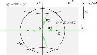
Figure 4: Local setup

Uniform exponential convergence in step 6 is the heart of the proof. It relies on a suitable time decomposition of trajectories. Throughout assume

Hypothesis 2

Assume the local setup of Hypothesis 1; see Figure 4. Consider the constants $\rho_{0}>0$ and $\kappa_{*}\geq 1$ and the continuous function $\kappa(\rho)$ with $\kappa(0)=0$ provided by the Lipschitz Lemma 1. Note that ${\mathcal{B}}_{\rho_{0}}\subset{\mathcal{U}}$. Fix $\mu$ in the spectral gap $(0,d)$ given by (4) and a constant $c=c(\mu)\geq 1$ satisfying Proposition 1 for the (finitely many) choices of $(\ell,k,r,q)$ that will be used in the present proof. We may assume that 

$$\rho_{0}c^{2}\kappa_{*}\left(\frac{1}{\mu}+\frac{8}{\mu^{\frac{1}{4}}}+\frac{6}{\mu^{\frac{5}{4}}}\right)\leq\frac{1}{8}.$$ (18)

In Hypothesis 1 (b) we picked $\varkappa\in(0,\rho_{0})$ and so the constant 

$$T_{1}=T_{1}(\varkappa,\mu,\rho_{0}):=-\frac{2}{\mu}\ln\frac{\varkappa}{\rho_{0}}>0$$ (19)

is well defined. Assume $\rho\in(0,\frac{1}{2}\rho_{0}]$ is sufficiently small such that

$$c^{2}\kappa(\rho)\left(\frac{9}{\mu^{\frac{1}{4}}}+\frac{4}{3\mu}+\frac{3}{\mu^{\frac{5}{4}}}\right)\leq\frac{1}{8}$$ (20)

and such that all points of ${\mathcal{U}}$ of distance $\leq\rho$ to the descending sphere $S^{u}_{\varepsilon}$ are contained in ${\mathcal{B}}_{\rho_{0}}$. Fix a constant $T_{2}=T_{2}(c,\mu,\rho,{\varepsilon})\geq 0$ such that $8ce^{-\mu T_{2}/4}\leq 1$ and $\phi_{-T_{2}/8}W^{u}_{\varepsilon}\subset{\mathcal{B}}^{-}:={\mathcal{B}}_{\rho/2c}\cap X^{-}$; see Remark 5.  Set $T_{0}:=\max\{T_{1},T_{2}\}>0$.

Pick $T\geq T_{0}$ and $\gamma\in S^{u}_{\varepsilon}$ and consider the infinite dimensional disk ${\mathcal{D}}_{\gamma}=\{\gamma\}\times{\mathcal{B}}^{+}_{\varkappa}$. The key observation to represent the preimage ${\phi_{T}}^{-1}{\mathcal{D}}_{\gamma}$ under the time-$T$-map $\phi_{T}$ as a graph over the stable subspace $X^{+}$ is the fact that to any pair $(q_{u},z_{+})\in X^{-}\oplus X^{+}$ sufficiently close to zero there corresponds a unique heat flow trajectory $\xi$ whose initial value $\xi(0)$ projects under $\pi_{+}$ to $z_{+}$ and whose endpoint at time $T$ projects under $\pi_{-}$ to $q_{u}$; see Remark 3. In particular, for $q_{u}:=\gamma$ any $z_{+}\in X^{+}$ near the origin corresponds to a unique heat flow line $\xi=\xi^{T}_{\gamma,z_{+}}$ which ends at time $T$ in ${\mathcal{D}}_{\gamma}$. Because its initial value $\xi(0)$ is of the form $\left(\pi_{-}\xi(0),z_{+}\right)$, it is natural to define the map $G^{T}_{\gamma}(z_{+}):=\pi_{-}\xi(0)$ whose graph at $z_{+}$ reproduces $\xi(0)$. In fact, we prove that for any $z_{+}\in X^{+}$ with $\mathopen{\|}z_{+}\mathclose{\|}\leq\rho/2c$ there is precisely one semi-flow line $\xi=\xi_{\gamma,z_{+}}^{T}$ with initial condition $\pi_{+}\xi(0)=z_{+}$ and endpoint condition $\xi(T)\in{\mathcal{D}}_{\gamma}$. The latter is equivalent to

$$\pi_{-}\xi(T)=\gamma\quad\wedge\quad\left\|\xi(T)-\gamma\right\|_{X}\leq\varkappa.$$ (21)

We will see in step 2 that the definition of $T_{1}$ assures the second condition.

The key step to determine the unique semi-flow line $\xi$ associated to $(T,\gamma,z_{+})$ is to set up a strict contraction on a complete metric space $Z^{T}$ whose (unique) fixed point is $\xi$. Set

$$\left\|\xi\right\|_{\exp}=\left\|\xi\right\|_{\exp,T}:=\max_{s\in[0,T]}e^{s\frac{\mu}{2}}\left\|\xi(s)\right\|_{X}$$ (22)

and for $\gamma_{T}:=\phi_{-T}\gamma$ define

$$Z^{T}=Z^{T,\gamma}_{\mu/2,\rho}:=\left\{\xi\in C^{0}([0,T],X)\,\colon\left\|\xi-\phi_{\cdot}\gamma_{T}\right\|_{\exp}\leq\rho\right\}.$$ (23)

Consider the map $\Psi^{T}=\Psi^{T}_{\gamma,z_{+}}$ defined on $Z^{T}$ by

$$\begin{split}\left(\Psi_{\gamma,z_{+}}^{T}\xi\right)(s)&:=e^{-sA}z_{+}+\int_{0}^{s}e^{-(s-\sigma)A}\pi_{+}f(\xi(\sigma))\,d\sigma\\ &\quad+e^{-(s-T)A^{-}}\gamma-\int_{s}^{T}e^{-(s-\sigma)A^{-}}\pi_{-}f(\xi(\sigma))\,d\sigma\end{split}$$ (24)

for every $s\in[0,T]$. The fixed points of $\Psi^{T}$ correspond to the desired heat flow trajectories by Proposition 2. By step 1 and step 2 below $\Psi^{T}$ is a strict contraction on $Z^{T}$. Hence by the Banach fixed point theorem it admits a unique fixed point $\xi_{\gamma,z_{+}}^{T}$ and for ${\mathcal{B}}^{+}:={\mathcal{B}}^{+}_{\rho/2c}\subset X^{+}$ we define the map

$$G^{T}:S^{u}_{\varepsilon}\times{\mathcal{B}}^{+}\to W^{u}\subset X^{-},\qquad\left(\gamma,z_{+}\right)\mapsto\pi_{-}\xi_{\gamma,z_{+}}^{T}(0)=:G^{T}_{\gamma}(z_{+}).$$ (25)

Actually ${\mathcal{B}}^{+}$ is the same ball for which the stable manifold Theorem 2.1 holds true Joa-LOOPSPACE .

The proof takes six steps. Fix $\gamma\in S^{u}_{\varepsilon}$ and $z_{+}\in{\mathcal{B}}^{+}$ and abbreviate $\Psi^{T}=\Psi_{\gamma,z_{+}}^{T}$.

Step 1. Fix $T\geq 0$. Then the set $Z^{T}$ equipped with the metric induced by the exp norm is a complete metric space, any $\xi\in Z^{T}$ takes values in ${\mathcal{B}}_{\rho_{0}}$, and $\Psi^{T}$ acts on $Z^{T}$.

Proof

In case of the compact domain $[0,T]$ the space $C^{0}([0,T],X)$ is complete with respect to the supremum norm, hence with respect to the exp norm as both norms are equivalent by compactness of $[0,T]$. The subset $Z^{T}\subset C^{0}([0,T],X)$ is closed with respect to the exp norm. By the assumption which immediately follows (20) the elements of $Z^{T}$ take values in ${\mathcal{B}}_{\rho_{0}}$, hence in ${\mathcal{U}}$.

To see that $\Psi^{T}$ acts on $Z^{T}$ we need to verify that $\Psi^{T}\xi$ is continuous and satisfies the exponential decay condition in (23) whenever $\xi\in Z^{T}$. By definition $\Psi^{T}\xi$ is a sum of four terms. That each one is continuous as a map $[0,T]\to X$ is standard. For terms one, two, and four see step 1 (iii) in the proof of Theorem 2.1 given in Joa-LOOPSPACE . For term three continuity follows from the definition of the exponential by the power series (12). For latter reference we sketch the argument for term two which we denote by $F(s)$: Continuity of $F:[0,T]\to X$ and the fact that $F(0)=0$ (used in steps 2 and 3 below) both follow by an analogue of (Joa-HABILITATION, , Le. 9.7 a)) for $-A$ instead of $\Delta$ and with $p=2$; see also (Henry-81-GeomTheory, , Le. 3.2.1). The condition to be checked is that the map $\tilde{f}:=\pi_{+}\circ f\circ\xi:[0,T]\to Y^{+}\hookrightarrow Y$ is continuous and bounded: This is true since $\xi:[0,T]\to X$ is continuous and bounded by definition of $Z^{T}$ and so is $f$ by Lemma 1.

We prove exponential decay. For $s\in[0,T]$ consider the heat flow trajectory given by $\phi_{s}\gamma_{T}$. By the representation formula of Proposition 2 it satisfies

$$\begin{split}\phi_{s}\gamma_{T}&=\int_{0}^{s}e^{-(s-\sigma)A}\pi_{+}f(\phi_{\sigma}\gamma_{T})\,d\sigma+e^{-(s-T)A^{-}}\gamma-\int_{s}^{T}e^{-(s-\sigma)A^{-}}\pi_{-}f(\phi_{\sigma}\gamma_{T})\,d\sigma.\end{split}$$ (26)

Here we used that $\pi_{+}\gamma_{T}=0$, because $\gamma$ and therefore $\gamma_{T}=\phi_{-T}\gamma$ lies in $W^{u}(0,{\mathcal{U}})\subset X^{-}$ by backward flow invariance. By the same argument $\pi_{-}\phi_{T}\gamma_{T}=\pi_{-}\gamma=\gamma$. By definition (24) of $\Psi^{T}$ and (26) we get for $s\in[0,T]$ the estimate

$$\begin{split}&\left\|\left(\Psi^{T}\xi\right)(s)-\phi_{s}\gamma_{T}\right\|_{X}\\ &\leq\left\|e^{-sA}z_{+}\right\|_{X}+\int_{0}^{s}\left\|e^{-(s-\sigma)A}\pi_{+}\right\|_{{\mathcal{L}}(Y,X)}\left\|f(\xi(\sigma))-f(\phi_{\sigma}\gamma_{T})\right\|_{Y}d\sigma\\ &\quad+\int_{s}^{T}\left\|e^{-(s-\sigma)A^{-}}\pi_{-}\right\|_{{\mathcal{L}}(Y,X)}\left\|f(\xi(\sigma))-f(\phi_{\sigma}\gamma_{T})\right\|_{Y}d\sigma\\ &\leq ce^{-s\mu}\left\|z_{+}\right\|_{X}+c\kappa(\rho)e^{-s\frac{\mu}{2}}\left\|\xi-\phi_{\cdot}\gamma_{T}\right\|_{\exp}\int_{0}^{s}\frac{e^{-(s-\sigma)\frac{\mu}{2}}}{(s-\sigma)^{\frac{3}{4}}}\,d\sigma\\ &\quad+c\kappa(\rho)e^{-s\frac{\mu}{2}}\left\|\xi-\phi_{\cdot}\gamma_{T}\right\|_{\exp}\int_{s}^{T}e^{(s-\sigma)\frac{3}{2}\mu}\,d\sigma\\ &\leq\frac{\rho}{2}e^{-s\mu}+c\kappa(\rho)\left(\frac{8}{\mu^{1/4}}+\frac{2}{3\mu}\right)\rho e^{-s\frac{\mu}{2}}\leq\rho e^{-s\frac{\mu}{2}}\end{split}$$ (27)

where the last inequality is by smallness (20) of $\rho$. Inequality two follows by the exponential decay Proposition 1 with constant $c$ and the Lipschitz Lemma 1 for $f$ with Lipschitz constant $\kappa(\rho)$. We multiplied the integrands by $e^{-\sigma\frac{\mu}{2}}e^{\sigma\frac{\mu}{2}}$ to create the exp norms. Inequality three uses $\mathopen{\|}z_{+}\mathclose{\|}_{X}\leq\frac{\rho}{2c}$ and boundedness of the exp norms by $\rho$ since $\xi\in Z^{T}$. We also used that

$$\int_{s}^{\infty}e^{(s-\sigma)\frac{3}{2}\mu}\,d\sigma=\frac{2}{3\mu}.$$ (28)

To estimate the other integral define $\Gamma(\alpha):=\int_{0}^{\infty}e^{-\tau}\tau^{\alpha-1}\,d\tau$ for $\alpha>0$. The $\Gamma$ function satisfies $\Gamma(\frac{1}{4})=4\Gamma(\frac{5}{4})\leq 4$ since $\Gamma\leq 1$ on the interval $[1,2]$. Hence

$$\int_{0}^{s}\frac{e^{-(s-\sigma)\frac{\mu}{2}}}{(s-\sigma)^{\frac{3}{4}}}\,d\sigma=\left(\frac{2}{\mu}\right)^{\frac{1}{4}}\int_{0}^{s\frac{\mu}{2}}e^{-\tau}\tau^{\frac{1}{4}-1}\,d\tau\leq\frac{2^{\frac{1}{4}}}{\mu^{\frac{1}{4}}}\,\Gamma(\tfrac{1}{4})\leq\frac{8}{\mu^{\frac{1}{4}}}.$$ (29)

∎

Step 2. For $T\geq 0$ the map $\Psi^{T}$ acts as a strict contraction on $Z^{T}$. Each image point $\Psi^{T}\xi$ satisfies the initial condition $\pi_{+}\left(\Psi^{T}\xi\right)(0)=z_{+}$ and, if $T\geq T_{1}$, also the endpoint condition (21), that is $\left(\Psi^{T}\xi\right)(T)\in{\mathcal{D}}_{\gamma}=\{\gamma\}\times{\mathcal{B}}^{+}_{\varkappa}$.

Proof

Assume $T\geq 0$ and fix $\xi_{1},\xi_{2}\in Z^{T}$. Similarly to (27) we obtain that

$$\begin{split}&\left\|\left(\Psi^{T}\xi_{1}\right)(s)-\left(\Psi^{T}\xi_{2}\right)(s)\right\|_{X}\\ &\leq\int_{0}^{s}\left\|e^{-(s-\sigma)A}\pi_{+}\right\|_{{\mathcal{L}}(Y,X)}\left\|f(\xi_{1}(\sigma))-f(\xi_{2}(\sigma))\right\|_{Y}d\sigma\\ &\quad+\int_{s}^{T}\left\|e^{-(s-\sigma)A^{-}}\pi_{-}\right\|_{{\mathcal{L}}(Y,X)}\left\|f(\xi_{1}(\sigma))-f(\xi_{2}(\sigma))\right\|_{Y}d\sigma\\ &\leq c\kappa(\rho)\left(\frac{8}{\mu^{1/4}}+\frac{2}{3\mu}\right)e^{-s\frac{\mu}{2}}\left\|\xi_{1}-\xi_{2}\right\|_{\exp}\end{split}$$ (30)

for every $s\in[0,T]$. Now use the smallness assumption (20) on $\rho$ to conclude that $\mathopen{\|}\Psi^{T}\xi_{1}-\Psi^{T}\xi_{2}\mathclose{\|}_{\exp}\leq\frac{1}{2}\mathopen{\|}\xi_{1}-\xi_{2}\mathclose{\|}_{\exp}$.

The identities $\pi_{+}\left(\Psi^{T}\xi\right)(0)=z_{+}$ and $\pi_{-}\left(\Psi^{T}\xi\right)(T)=\gamma$ follow from definition (24) of $\Psi^{T}$, the identities $\pi_{+}\pi_{-}=\pi_{-}\pi_{+}=0$, strong continuity of the semigroups on $X^{-}$ and $X^{+}$ asserted by Proposition 1, continuity and boundedness of both integrands, and $F(0)=0$ by the proof of step 1. Concerning the second endpoint condition in (21) assume $T\geq T_{1}$ and evaluate (27) at $s=T$ to get

$$\left\|\left(\Psi\xi\right)(T)-\gamma\right\|_{X}\leq\rho e^{-T\frac{\mu}{2}}\leq e^{-T_{1}\frac{\mu}{2}}\rho_{0}=\varkappa$$

where the last step is by definition of $T_{1}$ in (19). ∎

Step 3. For $T\geq 0$ the map $G^{T}:S^{u}_{\varepsilon}\times{\mathcal{B}}^{+}\to X^{-}$ defined by (25) is of class $C^{1}$ and, for each $\gamma\in S^{u}_{\varepsilon}$, the map $G^{T}_{\gamma}:=G^{T}(\gamma,\cdot):{\mathcal{B}}^{+}\to X^{-}$ satisfies

$$G^{T}_{\gamma}(0)=\phi_{-T}\gamma=:\gamma_{T},\qquad\mathrm{graph}\,G^{T}_{\gamma}=\left\{\xi_{\gamma,z_{+}}^{T}(0)\,\big{|}\,z_{+}\in{\mathcal{B}}^{+}\right\}.$$

Proof

Assume $T\geq 0$. By step 2 and its proof the map

$$\Psi^{T}:S^{u}_{\varepsilon}\times{\mathcal{B}}^{+}\times Z^{T}\to Z^{T},\qquad(\gamma,z_{+},\xi)\mapsto\Psi^{T}_{\gamma,z_{+}}\xi$$

is a uniform contraction on $Z^{T}$ with contraction factor $\tfrac{1}{2}$. (Actually $Z^{T}$ depends on $\gamma$, but the complete metric spaces associated to different $\gamma$’s are quasi-isometric.) Observe that $\Psi^{T}$ is linear, hence smooth, in $\gamma$ and in $z_{+}$ and of class $C^{1}$ in $\xi$, because $f$ is of class $C^{1}$ by the Lipschitz Lemma 1. Hence by the uniform contraction principle, see e.g. Chow-Hale-Bifurcation-Theory , the map $\lambda:S^{u}_{\varepsilon}\times{\mathcal{B}}^{+}\to Z^{T}$ assigning to $(\gamma,z_{+})$ the unique fixed point $\xi^{T}_{\gamma,z_{+}}$ of $\Psi^{T}_{\gamma,z_{+}}$ is of class $C^{1}$. So is its composition with (linear) evaluation $ev_{0}:Z^{T}\to X$, $\xi\mapsto\xi(0)$, and (linear) projection $\pi_{-}:X\to X^{-}$. But overall this composition is $G^{T}$ by definition (25). This proves that $G^{T}$, thus ${\mathcal{G}}$, is of class $C^{1}$ in $\gamma$ and $z_{+}$.

Consider the heat flow trajectory $\tilde{\eta}:[0,T]\to X$, $s\mapsto\phi_{s}\gamma_{T}=\phi_{s-T}\gamma$. By Remark 5 it takes values in $X^{-}$, because $\tilde{\eta}(T)=\gamma\in S^{u}_{\varepsilon}={\partial}W^{u}_{\varepsilon}\subset W^{u}$ lies in a descending disk. Hence $\pi_{+}\tilde{\eta}(0)=0$ and $\pi_{-}$ leaves $\tilde{\eta}$ pointwise invariant. An argument as in Remark 5 (using likewise forward uniqueness) shows that $\tilde{\eta}=\xi^{T}_{\gamma,0}$. Thus $G^{T}_{\gamma}(0):=\pi_{-}\xi^{T}_{\gamma,0}(0)=\pi_{-}\tilde{\eta}(0)=\tilde{\eta}(0)=\gamma_{T}$. To get the desired representation of $\mathrm{graph}\,G^{T}_{\gamma}$ observe that

$${\mathcal{G}}^{T}_{\gamma}(z_{+}):=\left(G^{T}_{\gamma}(z_{+}),z_{+}\right)=\left(\pi_{-}\xi^{T}_{\gamma,z_{+}}(0),\pi_{+}\xi^{T}_{\gamma,z_{+}}(0)\right)=\xi^{T}_{\gamma,z_{+}}(0)$$ (31)

by definition (25). The first identity also uses the fixed point property and the initial condition proved in step 2. The final identity is by $\pi_{-}\oplus\pi_{+}={{\mathchoice{\rm 1\mskip-4.0mul}{\rm 1\mskip-4.0mul}{\rm 1\mskip-4.5mul}{\rm 1\mskip-5.0mul}}}_{Y}$. ∎

Step 4. The map ${\mathcal{G}}$ is of class $C^{1}$. The map $T\mapsto{\mathcal{G}}(T,\gamma,z_{+})$ is Lipschitz continuous and its derivative is locally Hölder continuous with exponent $\alpha=\frac{1}{8}$. The map $\gamma\mapsto{\mathcal{G}}(T,\gamma,z_{+})$ is Lipschitz continuous.

Proof

By step 3 the map ${\mathcal{G}}$ is of class $C^{1}$ in the $\gamma$ and $z_{+}$ variables. By compactness of the $(k-1)$-dimensional sphere $S^{u}_{\varepsilon}$, the derivative of ${\mathcal{G}}$ with respect to $\gamma$ is bounded. Thus ${\mathcal{G}}$ is Lipschitz continuous in $\gamma$.

We prove that ${\mathcal{G}}$ is Lipschitz continuous in $T$. Fix $T\geq T_{0}>0$, $\gamma\in S^{u}_{\varepsilon}$, and $z_{+}\in{\mathcal{B}}^{+}$. The fixed point $\xi^{T}:=\xi^{T}_{\gamma,z_{+}}$ of $\Psi^{T}$ is given by (24) and the one of $\Psi^{T+\tau}$ by

$$\begin{split}\xi^{T+\tau}(s):=\xi^{T+\tau}_{\gamma,z_{+}}(s)&=e^{-sA}z_{+}+\int_{0}^{s}e^{-(s-\sigma)A}\pi_{+}f(\xi^{T+\tau}(\sigma))\,d\sigma\\ &\quad+e^{-(s-T-\tau)A^{-}}\gamma-\int_{s}^{T+\tau}e^{-(s-\sigma)A^{-}}\pi_{-}f(\xi^{T+\tau}(\sigma))\,d\sigma.\end{split}$$

For $s\in[0,T]$ and $\tau\geq 0$ we obtain, analogously to (27), the estimate

$$\begin{split}&\left\|\xi^{T+\tau}(s)-\xi^{T}(s)\right\|_{X}\\ &\leq\int_{0}^{s}\bigl{\|}e^{-(s-\sigma)A}\pi_{+}\bigr{\|}_{{\mathcal{L}}(Y,X)}\left\|f(\xi^{T+\tau}(\sigma))-f(\xi^{T}(\sigma))\right\|_{Y}\,d\sigma+\bigl{\|}\bigl{(}e^{\tau A^{-}}-{{\mathchoice{\rm 1\mskip-4.0mul}{\rm 1\mskip-4.0mul}{\rm 1\mskip-4.5mul}{\rm 1\mskip-5.0mul}}}\bigr{)}e^{-(s-T)A^{-}}\gamma\bigr{\|}_{X}\\ &\quad+\int_{s}^{T}\bigl{\|}e^{-(s-\sigma)A^{-}}\pi_{-}\bigr{\|}_{{\mathcal{L}}(Y,X)}\left\|f(\xi^{T+\tau}(\sigma))-f(\xi^{T}(\sigma))\right\|_{Y}\,d\sigma\\ &\quad+\int_{T}^{T+\tau}\bigl{\|}e^{-(s-\sigma)A^{-}}\pi_{-}\bigr{\|}_{{\mathcal{L}}(Y,X)}\left\|f(\xi^{T+\tau}(\sigma))\right\|_{Y}\,d\sigma\\ &\leq c\kappa(\rho)\left\|\xi^{T+\tau}-\xi^{T}\right\|_{C^{0}([0,T],X)}\left(\int_{0}^{s}\frac{e^{-(s-\sigma)\mu}}{(s-\sigma)^{\frac{3}{4}}}\,d\sigma+\int_{s}^{T}e^{(s-\sigma)\mu}\,d\sigma\right)\\ &\quad+\tau c\mathopen{|}\lambda_{1}\mathclose{|}\cdot ce^{(s-T)\mu}\left\|\gamma\right\|_{X}+c\kappa(\rho)\rho_{0}\int_{T}^{T+\tau}e^{(s-\sigma)\mu}\,d\sigma\\ &\leq c\kappa(\rho)\left(\frac{8}{\mu^{1/4}}+\frac{1}{\mu}\right)\left\|\xi^{T+\tau}-\xi^{T}\right\|_{C^{0}([0,T],X)}+\tau\rho_{0}c^{2}\mathopen{|}\lambda_{1}\mathclose{|}e^{(s-T)\mu}\\ &\quad+c\kappa(\rho)\rho_{0}\frac{e^{(s-T)\mu}}{\mu}\left(1-e^{-\tau\mu}\right)\\ &\leq\frac{1}{8}\left\|\xi^{T+\tau}-\xi^{T}\right\|_{C^{0}([0,T],X)}+\tau\rho_{0}\left(c^{2}\mathopen{|}\lambda_{1}\mathclose{|}+1\right)e^{(s-T)\mu}.\end{split}$$

Inequality two uses the Lipschitz Lemma 1 for $f$ and the exponential estimates of Proposition 1. To estimate the second of the four terms recall that $X^{-}$ is spanned by an orthonormal basis of eigenvectors of $A^{-}\in{\mathcal{L}}(X^{-})$ corresponding to the eigenvalues $\lambda_{1}\leq\ldots\leq\lambda_{k}<0$. Hence $\mathopen{\|}A^{-}\mathclose{\|}=-\lambda_{1}=\mathopen{|}\lambda_{1}\mathclose{|}$. Since $e^{-s\mu}\leq 1$ we get that

$$\frac{1-e^{-\mu\tau}}{\mu}=\int_{0}^{\tau}e^{-s\mu}\;ds\leq\tau.$$ (32)

Thus (LUNARDI-InetSem, , Prop. 1.3.6. (ii)) implies the estimate

$$\mathopen{\|}e^{\tau A^{-}}-{{\mathchoice{\rm 1\mskip-4.0mul}{\rm 1\mskip-4.0mul}{\rm 1\mskip-4.5mul}{\rm 1\mskip-5.0mul}}}\mathclose{\|}_{{\mathcal{L}}(X^{-})}=\left\|A^{-}\int_{0}^{\tau}e^{\sigma A^{-}}\,d\sigma\right\|_{{\mathcal{L}}(X^{-})}\leq\mathopen{|}\lambda_{1}\mathclose{|}\int_{0}^{\tau}ce^{-\sigma\mu}\,d\sigma\leq\tau c\mathopen{|}\lambda_{1}\mathclose{|}.$$ (33)

Coming back to inequality two above, we used that $\xi^{T+\tau}\in Z^{T+\tau}$ in term four takes values in ${\mathcal{B}}_{\rho_{0}}$ by step 1. Inequality three uses (29) and (28) for the first two integrals and that $\gamma\in S^{u}_{\varepsilon}\subset{\mathcal{B}}_{\rho_{0}}$. Inequality four uses (32) and smallness (20) of $\rho$ which also implies that $c\kappa(\rho)\leq 1$. Now set $c_{1}=2(c^{2}\mathopen{|}\lambda_{1}\mathclose{|}+1)$ and take the supremum over $s\in[0,T]$ to get that

$$\left\|\xi^{T+\tau}-\xi^{T}\right\|_{C^{0}([0,T],X)}\leq\rho_{0}c_{1}\tau.$$ (34)

Therefore by (31) we get $\mathopen{\|}{\mathcal{G}}^{T+\tau}_{\gamma}(z_{+})-{\mathcal{G}}^{T}_{\gamma}(z_{+})\mathclose{\|}_{X}=\mathopen{\|}\xi^{T+\tau}(0)-\xi^{T}(0)\mathclose{\|}_{X}\leq\rho_{0}c_{1}\tau$ and this proves that ${\mathcal{G}}(T,\gamma,z_{+})={\mathcal{G}}^{T}_{\gamma}(z_{+})$ is Lipschitz continuous in $T$. The difference $\xi^{T+\tau}-\xi^{T}$ is illustrated by Figure 5.

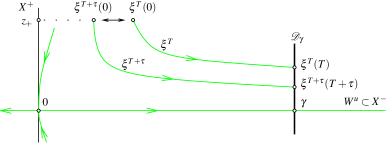
Figure 5: The difference ${\mathcal{G}}^{T+\tau}_{\gamma}(z_{+})-{\mathcal{G}}^{T}_{\gamma}(z_{+})$

We prove that $T\mapsto\frac{d}{dT}{\mathcal{G}}(T,\gamma,z_{+})$ is locally Hölder. Consider the derivative

$$\begin{split}\Theta^{T}(s)&:=\left.\tfrac{d}{d\tau}\right|_{\tau=0}\xi^{T+\tau}_{\gamma,z_{+}}(s)\\ &=\int_{0}^{s}e^{-(s-\sigma)A}\pi_{+}\bigl{(}df|_{\xi^{T}(\sigma)}\circ\Theta^{T}(\sigma)\bigr{)}d\sigma\;+\;A^{-}e^{-(s-T)A^{-}}\gamma\\ &\quad-e^{-(s-T)A^{-}}\pi_{-}f(\xi^{T}(T))-\int_{s}^{T}e^{-(s-\sigma)A^{-}}\pi_{-}\Bigl{(}df|_{\xi^{T}(\sigma)}\circ\Theta^{T}(\sigma)\Bigr{)}d\sigma.\end{split}$$

Since $\frac{d}{dT}{\mathcal{G}}(T,\gamma,z_{+})=\Theta^{T}(0)$ by (31), it remains to show that the map $T\mapsto\Theta^{T}(0)\in X$ is locally Hölder continuous. By definition of $\Theta^{T}$ we get the identity

$$\begin{split}\Theta^{T+\tau}(s)-\Theta^{T}(s)&=\int_{0}^{s}e^{-(s-\sigma)A}\pi_{+}df|_{\xi^{T+\tau}(\sigma)}\left(\Theta^{T+\tau}(\sigma)-\Theta^{T}(\sigma)\right)\,d\sigma\\ &\quad+\int_{0}^{s}e^{-(s-\sigma)A}\pi_{+}\left(df|_{\xi^{T+\tau}(\sigma)}-df|_{\xi^{T}}(\sigma)\right)\circ\Theta^{T}(\sigma)\,d\sigma\\ &\quad+\bigl{(}e^{\tau A^{-}}-{{\mathchoice{\rm 1\mskip-4.0mul}{\rm 1\mskip-4.0mul}{\rm 1\mskip-4.5mul}{\rm 1\mskip-5.0mul}}}\bigr{)}A^{-}e^{-(s-T)A^{-}}\gamma-\bigl{(}e^{\tau A^{-}}-{{\mathchoice{\rm 1\mskip-4.0mul}{\rm 1\mskip-4.0mul}{\rm 1\mskip-4.5mul}{\rm 1\mskip-5.0mul}}}\bigr{)}e^{-(s-T)A^{-}}\pi_{-}f(\xi^{T+\tau}(T+\tau))\\ &\quad-e^{-(s-T)A^{-}}\pi_{-}\left(f(\xi^{T+\tau}(T+\tau))-f(\xi^{T}(T))\right)\\ &\quad-\int_{s}^{T}e^{-(s-\sigma)A^{-}}\pi_{-}df|_{\xi^{T+\tau}(\sigma)}\left(\Theta^{T+\tau}(\sigma)-\Theta^{T}(\sigma)\right)\,d\sigma\\ &\quad-\int_{s}^{T}e^{-(s-\sigma)A^{-}}\pi_{-}\left(df|_{\xi^{T+\tau}(\sigma)}-df|_{\xi^{T}}(\sigma)\right)\circ\Theta^{T}(\sigma)\,d\sigma\\ &\quad-\int_{T}^{T+\tau}e^{-(s-\sigma)A^{-}}\pi_{-}df|_{\xi^{T+\tau}(\sigma)}\circ\Theta^{T+\tau}(\sigma)\,d\sigma\end{split}$$

for all $s\in[0,T]$ and $\tau\geq 0$. To obtain terms one and two we added zero, similarly for terms four and five and terms six and seven. Abbreviate the norm of the Banach space $C^{0}([0,T],X)$ by $\mathopen{\|}\cdot\mathclose{\|}_{C^{0}_{T}}$ and combine terms one and six and terms two and seven to get that

$$\begin{split}&\left\|\Theta^{T+\tau}(s)-\Theta^{T}(s)\right\|_{X}\\ &\leq c\kappa(\rho)\left\|\Theta^{T+\tau}-\Theta^{T}\right\|_{C^{0}_{T}}\left(\int_{0}^{s}\frac{e^{-(s-\sigma)\mu}}{(s-\sigma)^{\frac{3}{4}}}\,d\sigma+\int_{s}^{T}e^{(s-\sigma)\mu}\,d\sigma\right)\\ &\quad+c\kappa_{*}\left\|\xi^{T+\tau}-\xi^{T}\right\|_{C^{0}_{T}}\left\|\Theta^{T}\right\|_{C^{0}_{T}}\left(\int_{0}^{s}\frac{e^{-(s-\sigma)\mu}}{(s-\sigma)^{\frac{3}{4}}}\,d\sigma+\int_{s}^{T}e^{(s-\sigma)\mu}\,d\sigma\right)\\ &\quad+\tau c^{2}\mathopen{|}\lambda_{1}\mathclose{|}\left(\mathopen{|}\lambda_{1}\mathclose{|}\cdot\left\|\gamma\right\|_{X}+\kappa(\rho)\left\|\xi^{T+\tau}(T+\tau)\right\|_{X}\right)e^{(s-T)\mu}\\ &\quad+c\kappa(\rho)\left\|\xi^{T+\tau}(T+\tau)-\xi^{T}(T)\right\|_{X}e^{(s-T)\mu}+c\kappa(\rho)\left\|\Theta^{T+\tau}\right\|_{C^{0}_{T+\tau}}\int_{T}^{T+\tau}e^{(s-\sigma)\mu}\,d\sigma\\ &\leq c\kappa(\rho)\left(\frac{8}{\mu^{1/4}}+\frac{1}{\mu}\right)\left\|\Theta^{T+\tau}-\Theta^{T}\right\|_{C^{0}_{T}}+\tau c\kappa_{*}\rho_{0}^{2}c_{1}^{2}\left(\frac{8}{\mu^{1/4}}+\frac{1}{\mu}\right)\\ &\quad+\tau c\rho_{0}\mathopen{|}\lambda_{1}\mathclose{|}\left(c\mathopen{|}\lambda_{1}\mathclose{|}+1\right)+\tau^{\frac{1}{8}}\rho_{0}\left(c_{3}T^{\frac{3}{8}}+c_{4}\tau^{\frac{1}{8}}\right)+\frac{\rho_{0}c_{1}}{\mu}\left(1-e^{-\tau\mu}\right)\\ &\leq\frac{1}{8}\left\|\Theta^{T+\tau}-\Theta^{T}\right\|_{C^{0}_{T}}+\rho_{0}\left(\tau c_{1}^{2}+\tau c\mathopen{|}\lambda_{1}\mathclose{|}c_{1}+\tau^{\frac{1}{8}}\left(c_{3}T^{\frac{3}{8}}+c_{4}\tau^{\frac{1}{8}}\right)+\tau c_{1}\right)\end{split}$$

for $s\in[0,T]$ and $\tau\geq 0$. Inequality one uses the exponential decay Proposition 1, the Lipschitz Lemma 1 for $f$, and its Corollary 1. To obtain line three we used (33). In line five we used backward time exponential decay (13).
To see inequality two observe the following. Estimate the first integral in lines one and two by (29), the second one by (28). Recall that $\gamma\in{\mathcal{B}}_{\rho_{0}}$ by our local setup. Apply estimate (34). In addition, use (34) to conclude that $\mathopen{\|}\Theta^{T}(s)\mathclose{\|}_{X}\leq\rho_{0}c_{1}$ whenever $s\in[0,T]$. (Note that the same is true when $T$ is replaced by $T+\tau$.) The elements of $Z^{T}$ (and $Z^{T+\tau}$) take values in ${\mathcal{B}}_{\rho_{0}}$ by step 1. Use that $c\kappa(\rho)\leq 1$ by (20) and that $e^{(s-T)\mu}\leq 1$. To estimate the difference $\xi^{T+\tau}(T+\tau)-\xi^{T}(T)\in X$ in line four is surprisingly subtle. This estimate will be carried out separately below; see (36) for the result used in inequality two and for the definition of $c_{3}$ and $c_{4}$.
To obtain inequality three we used smallness (18) and (20) of $\rho$ and estimate (32). Now take the supremum over $s\in[0,T]$ to get

$$\left\|\Theta^{T+\tau}-\Theta^{T}\right\|_{C^{0}([0,T],X)}\leq c_{T}\rho_{0}\tau^{\frac{1}{8}}$$ (35)

where $\frac{1}{2}c_{T}=c_{3}T^{\frac{3}{8}}+\tau^{\frac{7}{8}}\left(c_{1}^{2}+c^{2}\lambda_{1}^{2}+c\mathopen{|}\lambda_{1}\mathclose{|}+c_{1}\right)+c_{4}\tau^{\frac{1}{8}}$. Thus

$$\left\|\tfrac{d}{dT}{\mathcal{G}}(T+\tau,\gamma,z_{+})-\tfrac{d}{dT}{\mathcal{G}}(T,\gamma,z_{+})\right\|_{X}=\left\|\Theta^{T+\tau}(0)-\Theta^{T}(0)\right\|_{X}\leq c_{T}\rho_{0}\tau^{\frac{1}{8}},$$

that is $T\mapsto\frac{d}{dT}{\mathcal{G}}(T,\gamma,z_{+})$ is locally Hölder continuous with exponent $\alpha=\frac{1}{8}$.

As mentioned above it remains to estimate the $W^{1,2}$ norm of the difference:

$$\begin{split}\xi^{T+\tau}(T+\tau)-\xi^{T}(T)&=\left(e^{-\tau A}-{{\mathchoice{\rm 1\mskip-4.0mul}{\rm 1\mskip-4.0mul}{\rm 1\mskip-4.5mul}{\rm 1\mskip-5.0mul}}}\right)e^{-TA}z_{+}\\ &\quad+\int_{0}^{T}e^{-(T+\tau-\sigma)A}\pi_{+}\left(f(\xi^{T+\tau}(\sigma))-f(\xi^{T}(\sigma))\right)\,d\sigma\\ &\quad+\int_{0}^{T}\left(e^{-\tau A}-{{\mathchoice{\rm 1\mskip-4.0mul}{\rm 1\mskip-4.0mul}{\rm 1\mskip-4.5mul}{\rm 1\mskip-5.0mul}}}\right)e^{-(T-\sigma)A}\pi_{+}f(\xi^{T}(\sigma))\,d\sigma\\ &\quad+\int_{T}^{T+\tau}e^{-(T+\tau-\sigma)A}\pi_{+}f(\xi^{T+\tau}(\sigma))\,d\sigma.\end{split}$$

We added zero to obtain terms II and III in this sum I+II+III+IV of four.

I) Concerning term one we get

$$\begin{split}\left\|\left(e^{-\tau A}-{{\mathchoice{\rm 1\mskip-4.0mul}{\rm 1\mskip-4.0mul}{\rm 1\mskip-4.5mul}{\rm 1\mskip-5.0mul}}}\right)e^{-TA}z_{+}\right\|_{X}&=\left\|\int_{0}^{\tau}-Ae^{-sA}e^{-TA}z_{+}\,ds\right\|_{X}\\ &\leq\int_{0}^{\tau}\left\|e^{-sA}\pi_{+}\right\|_{{\mathcal{L}}(X)}\left\|Ae^{-TA}\pi_{+}\right\|_{{\mathcal{L}}(X)}\left\|z_{+}\right\|_{X}\,ds\\ &\leq\int_{0}^{\tau}ce^{-s\mu}\left(\frac{c^{\prime}C}{T}e^{-T\mu}\right)\rho_{0}\,ds\\ &\leq\frac{cc^{\prime}C\rho_{0}e^{-T_{0}\mu}}{T_{0}}\;\tau.\end{split}$$

The first identity even without norms is standard; see e.g. (LUNARDI-InetSem, , Prop. 1.3.6. (ii)). To obtain inequality one we permuted $A$ and $e^{-sA}$; see e.g. (LUNARDI-InetSem, , Thm. 1.3.3. (i)). Here we used that $e^{-TA}z_{+}\in W^{2,1}=D(A)$ since $T>0$. Compare the above estimate on $X^{+}$ with the corresponding estimate (33) on the finite dimensional vector space $X^{-}$ and note how boundedness of $A^{-}$ simplifies (33). Inequality two uses that the norms $\mathopen{\|}A\cdot\mathclose{\|}_{1,2}$ and $\mathopen{\|}\cdot\mathclose{\|}_{3,2}$ are equivalent with constant $c^{\prime}$ by compactness of $S^{1}$ and $A$ being of second order. The regularity-for-singularity estimate (14) with constant $C=C(\mu)$ allows to get from $W^{3,2}$ back to $W^{1,2}$ catching a factor $CT^{-1}$. The final step uses (32).

II) For term two use estimate (34) and the fact that $c\kappa(\rho)\leq 1$ by (20) to get that

$$\begin{split}\int_{0}^{T}\left\|e^{-(T+\tau-\sigma)A}\pi_{+}\left(f(\xi^{T+\tau}(\sigma))-f(\xi^{T}(\sigma))\right)\right\|_{X}d\sigma&\leq\frac{\rho_{0}c_{1}\tau}{\mu^{\frac{1}{4}}}\int_{\tau\mu}^{\tau\mu+T\mu}\frac{e^{-s}}{s^{\frac{3}{4}}}ds\\ &\leq\frac{\rho_{0}c_{1}\tau}{\mu^{\frac{1}{4}}}\Gamma(\tfrac{1}{4})\\ &\leq\frac{4\rho_{0}c_{1}}{\mu^{\frac{1}{4}}}\;\tau.\end{split}$$

We also used the definition of the $\Gamma$ function after (28) and its functional equation.

III) Term three requires similar techniques as term one, but their application requires more care. Namely, it is crucial not to deal with the ${\mathcal{L}}(L^{1},W^{3,2})$ norm in one go, but to decompose it into a product involving ${\mathcal{L}}(L^{1},W^{1,q})$ and ${\mathcal{L}}(W^{1,q},W^{3,2})$ norms where $q$ is any real strictly larger than the order (two) of the differential operator $A$. This way we avoid catching either a factor $s^{-\alpha}$ or $T^{-\alpha}$ with $\alpha\geq 1$ when trading regularity for singularity via (14). Each of these factors would void our estimate, since they are not integrable locally near zero. Pick $q>2$. Similarly as in case of term one we obtain that

$$\begin{split}&\int_{0}^{T}\left\|\left(e^{-\tau A}-{{\mathchoice{\rm 1\mskip-4.0mul}{\rm 1\mskip-4.0mul}{\rm 1\mskip-4.5mul}{\rm 1\mskip-5.0mul}}}\right)e^{-(T-\sigma)A}\pi_{+}f(\xi^{T}(\sigma))\right\|_{X}\,d\sigma\\ &\leq\int_{0}^{T}\int_{0}^{\tau}\left\|Ae^{-sA}e^{-(T-\sigma)A}\pi_{+}f(\xi^{T}(\sigma))\right\|_{W^{1,2}}\,ds\,d\sigma\\ &\leq\int_{0}^{T}\int_{0}^{\tau}c^{\prime}\left\|e^{-sA}e^{-(T-\sigma)A}\pi_{+}f(\xi^{T}(\sigma))\right\|_{W^{3,2}}\,ds\,d\sigma\\ &\leq c^{\prime}\kappa(\rho)\rho_{0}\int_{0}^{T}\int_{0}^{\tau}\left\|e^{-sA}\pi_{+}\right\|_{{\mathcal{L}}(W^{1,q},W^{3,2})}\left\|e^{-(T-\sigma)A}\pi_{+}\right\|_{{\mathcal{L}}(L^{1},W^{1,q})}\,ds\,d\sigma\\ &\leq c^{\prime}C^{\prime}C^{\prime\prime}\rho_{0}\int_{0}^{\tau}e^{-s\mu}s^{-\frac{3}{4}-\frac{1}{2q}}\,ds\,\int_{0}^{T}e^{-(T-\sigma)\mu}(T-\sigma)^{-\frac{1}{2}-\frac{1}{2q}}\,d\sigma\\ &=c^{\prime}C^{\prime}C^{\prime\prime}\rho_{0}\int_{0}^{\tau}e^{-s\mu}s^{-\frac{7}{8}}\,ds\,\int_{0}^{T}e^{-s\mu}s^{-\frac{5}{8}}\,ds\\ &\leq 22c^{\prime}C^{\prime}C^{\prime\prime}\rho_{0}T^{\frac{3}{8}}\tau^{\frac{1}{8}}.\end{split}$$

Inequality three uses once more that $\mathopen{\|}\xi^{T}(\sigma))\mathclose{\|}_{X}\leq\rho_{0}$ by step 1. Note that $\kappa(\rho)\leq 1$. Inequality four uses twice the regularity-for-singularity estimate (14) with constants $C^{\prime}$ and $C^{\prime\prime}$, respectively. The exponent of $s$ shows that concerning integrability we could have picked any $q>2$. In the final inequality we dropped the factors $e^{-s\mu}\leq 1$ and carried out the integrals.

IV) Concerning term four we get the estimate

$$\int_{T}^{T+\tau}\left\|e^{-(T+\tau-\sigma)A}\pi_{+}f(\xi^{T+\tau}(\sigma))\right\|_{X}d\sigma\leq\rho_{0}\int_{0}^{\tau}e^{-s\mu}s^{-\frac{3}{4}}\,ds\leq 4\rho_{0}\tau^{\frac{1}{4}}$$

by dropping the term $e^{-s\mu}\leq 1$ under the integral.

Side remark concerning the estimate for term III: Unfortunately, we do not see any way to trade $\tau^{1/8}$ for $\tau$ or, equivalently, to trade $T^{3/8}$ for $T$. This has the following consequences. The positive power of $T$ obstructs the conclusion that $\frac{d}{dT}{\mathcal{G}}$ is uniformly continuous in $T$. The conclusion of local Lipschitz continuity is obstructed by the factor $\tau^{\alpha}$ with $\alpha=1/8<1$. All we can say is that $\frac{d}{dT}{\mathcal{G}}$ is locally Hölder continuous in $T$ with exponent $\alpha=1/8$.

To summarize, the above estimates show that

$$\left\|\xi^{T+\tau}(T+\tau)-\xi^{T}(T)\right\|_{X}\leq\tau^{\frac{1}{8}}\rho_{0}\left(c_{3}T^{\frac{3}{8}}+c_{4}\tau^{\frac{1}{8}}\right)$$ (36)

for $\tau\geq 0$ and where

$$c_{3}:=22c^{\prime}C^{\prime}C^{\prime\prime},\qquad c_{4}:=4+\tau^{\frac{7}{8}}\left(cc^{\prime}CT_{0}^{-1}+4c_{1}\mu^{-\frac{1}{4}}\right).$$

This concludes the proof of (35) and therefore of step 4. ∎

Step 5. For $T\geq 0$ the graph map ${\mathcal{G}}^{T}_{\gamma}:{\mathcal{B}}^{+}\to X^{-}\oplus X^{+}$, $z_{+}\mapsto\left(G^{T}_{\gamma}(z_{+}),z_{+}\right)$, and its inverse $\pi_{+}|_{{\mathcal{G}}^{T}_{\gamma}({\mathcal{B}}^{+})}$ are both Lipschitz continuous with respect to the $W^{1,2}$ norm. In fact, the graph map is a diffeomorphism onto its image.

Proof

For $j=1,2$ pick $z_{j}\in{\mathcal{B}}^{+}$ and denote the fixed point $\xi^{T}_{\gamma,z_{j}}$ of $\Psi^{T}=\Psi^{T}_{\gamma,z_{j}}$ by $\xi_{j}$. Similarly to the estimate in the proof of step 2 we obtain for each $s\in[0,T]$ that

$$\left\|\xi_{1}(s)-\xi_{2}(s)\right\|_{X}\leq ce^{-s\mu}\left\|z_{1}-z_{2}\right\|_{X}+\frac{1}{2}\left\|\xi_{1}-\xi_{2}\right\|_{\exp}.$$

Multiply by $e^{s\frac{\mu}{2}}$ and take the supremum over $s\in[0,T]$ to get

$$\left\|\xi_{1}-\xi_{2}\right\|_{\exp}\leq 2c\left\|z_{1}-z_{2}\right\|_{X}.$$ (37)

By (31) this proves Lipschitz continuity of ${\mathcal{G}}^{T}_{\gamma}$, namely

$$\left\|{\mathcal{G}}^{T}_{\gamma}(z_{1})-{\mathcal{G}}^{T}_{\gamma}(z_{2})\right\|_{X}=\left\|\xi_{1}(0)-\xi_{2}(0)\right\|_{X}\leq\left\|\xi_{1}-\xi_{2}\right\|_{\exp}\leq 2c\left\|z_{1}-z_{2}\right\|_{X}.$$

Next use that $\pi_{+}$ vanishes on $X^{-}$ and acts as the identity on $X^{+}$ to see that $\pi_{+}$ is a left inverse of ${\mathcal{G}}^{T}_{\gamma}$. Thus $\pi_{+}$ restricted to ${\mathcal{G}}^{T}_{\gamma}({\mathcal{B}}^{+})$ is its inverse. But this restriction is of class $C^{1}$, because it is of the form $\pi_{+}\circ{\mathcal{G}}^{T}_{\gamma}(z_{+})$ where $\pi_{+}$ is linear and the map $z_{+}\mapsto{\mathcal{G}}^{T}_{\gamma}(z_{+}):=\left(G^{T}_{\gamma}z_{+},z_{+}\right)$ is of class $C^{1}$ by step 3.

To see that the restriction of $\pi_{+}$ to ${\mathcal{G}}^{T}_{\gamma}({\mathcal{B}}^{+})$ is Lipschitz continuous consider the difference $\xi_{1}(0)-\xi_{2}(0)=\Psi^{T}\xi_{1}(0)-\Psi^{T}\xi_{2}(0)$ whose right hand side is given by (24). Apply $\mathopen{\|}a-b\mathclose{\|}\geq\mathopen{\|}a\mathclose{\|}-\mathopen{\|}b\mathclose{\|}$ with $a=z_{1}-z_{2}$ and (30) for $s=0$ to get

$$\left\|\xi_{1}(0)-\xi_{2}(0)\right\|_{X}\geq\left\|z_{1}-z_{2}\right\|_{X}-c\kappa(\rho)\frac{2}{3\mu}\left\|\xi_{1}-\xi_{2}\right\|_{\exp}.$$

By (37) and the smallness assumption (20) on $\rho$ this implies that

$$\left\|\xi_{1}(0)-\xi_{2}(0)\right\|_{X}\geq\left(1-c\kappa(\rho)\frac{2}{3\mu}2c\right)\left\|z_{1}-z_{2}\right\|_{X}\geq\frac{1}{2}\left\|z_{1}-z_{2}\right\|_{X}$$

which by (31) and the fact that $\pi_{+}$ left inverts ${\mathcal{G}}^{T}_{\gamma}$ is equivalent to

$$\left\|{\mathcal{G}}^{T}_{\gamma}(z_{1})-{\mathcal{G}}^{T}_{\gamma}(z_{2})\right\|_{X}\geq\frac{1}{2}\left\|\pi_{+}{\mathcal{G}}^{T}_{\gamma}(z_{1})-\pi_{+}{\mathcal{G}}^{T}_{\gamma}(z_{2})\right\|_{X}.$$ (38)

This proves that $\pi_{+}$ is Lipschitz continuous on the image of ${\mathcal{G}}^{T}_{\gamma}$.

By estimate (38) and the estimate after (37) the map ${\mathcal{G}}^{T}_{\gamma}$ is bi-Lipschitz and therefore a homeomorphism onto its image. Since the map and its inverse are both of class $C^{1}$, it is in fact a diffeomorphism onto its image. ∎

Step 6. (Uniform convergence) $\mathopen{\|}{\mathcal{G}}^{\infty}(z_{+})-{\mathcal{G}}_{\gamma}^{T}(z_{+})\mathclose{\|}_{W^{2,2}}\leq\rho_{0}e^{-T\frac{\mu}{16}}$ $\forall T\geq T_{2}$.

Proof

Assume $T\geq T_{2}$; see (39) below. Consider the fixed point $\xi^{T}=\xi^{T}_{\gamma,z_{+}}$ of $\Psi_{\gamma,z_{+}}^{T}$ on $Z^{T}$ and the fixed point $\eta=\eta_{z_{+}}$ of $\Psi_{z_{+}}$ on $Z$ defined by (17). Because ${\mathcal{G}}^{T}_{\gamma}(z_{+})=\xi^{T}(0)$ by (31), similarly ${\mathcal{G}}^{\infty}(z_{+})=\eta(0)$, it remains to estimate the difference $\eta(0)-\xi^{T}(0)$. Observe that, firstly, since the difference lies in $X^{-}\subset C^{\infty}$ application of the $W^{2,2}$ norm makes sense. Secondly, by the respective representation formulae, this difference depends on the whole trajectories $\eta$ and $\xi^{T}$. But while $\eta$ runs into the origin, the trajectory $\xi^{T}$ ends on the fiber ${\mathcal{D}}_{\gamma}$ far away! So the difference $\eta-\xi^{T}$ cannot converge to zero, as $T\to\infty$, uniformly on $[0,T]$. However, Figure 5 suggests that this could be true on some initial part of the domain $[0,T]$, say on $[0,\frac{1}{2}T]$. So step A is to reduce the problem to the smaller interval $[0,\frac{1}{2}T]$. Step B is to solve the reduced problem. Here the key idea is to suitably partition both trajectories $\eta$ and $\xi^{T}$ and compare due parts; see Figure 6. The fact that $\eta$ is asymptotically well behaved, i.e. exponentially close to zero on $[T,\infty)$, enters frequently.

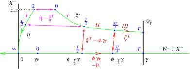
Figure 6: Time partitions and exponentially decaying differences

We proceed as follows: In step A we estimate the (stronger) $W^{2,2}$ norm of the difference $\eta(0)-\xi^{T}(0)$ by an exponentially decaying function of $T$ plus the supremum over $s\in[0,\frac{1}{2}T]$ of the (weaker) norm $\mathopen{\|}\eta(s)-\xi^{T}(s)\mathclose{\|}_{X}$. This reduction of a stronger to a weaker norm is based on the key fact that the difference $\eta(0)-\xi^{T}(0)$ only involves $\pi_{-}$ terms. Namely, these take values in $X^{-}$, hence in $C^{\infty}$. In step B we prove exponential decay of this sup norm. Here we encounter again the difference $\eta-\xi^{T}$, unfortunately on the whole interval $[0,T]$. Now the key idea is to decompose this interval into three pieces, namely

$$I:=[0,\tfrac{1}{2}T],\qquad II:=[\tfrac{1}{2}T,\tfrac{3}{4}T],\qquad III:=[\tfrac{3}{4}T,T],$$

as shown in Figure 6. In fact an extra piece $[T,\infty)$ is brought in by $\eta$. On interval $I$ we pull out the supremum norm and use smallness of the Lipschitz constant $\kappa(\rho)$ to get a coefficient less than one to throw the whole $(\eta-\xi^{T})$ term on the left hand side. Off $I$ we apply the triangle inequality to deal with each term $\eta$ and $\xi^{T}$ separately. Exponential decay built into the definition (17) of $Z$ allows to handle $\eta$ on its whole remaining time interval $[\frac{1}{2}T,\infty)$ in one go. It remains to deal with $\xi^{T}$ on intervals $II$ and $III$. For $\sigma\in II$ we exploit (after adding zero) that both terms $\xi^{T}(\sigma)-\phi_{\sigma}(\gamma_{T})$ and $\phi_{\sigma}(\gamma_{T})$ individually decay exponentially in $T$, uniformly in $\sigma\in II$. For the first term this is simply true by definition (23) of $Z^{T}$. Concerning the second term we use that $\gamma$ lies in the unstable manifold. Hence $\phi_{\sigma}(\gamma_{T})=\phi_{t}(\gamma)$ collapses exponentially fast into the origin, since $t:=\sigma-T\in[-\frac{1}{2}T,-\frac{1}{4}T]$ and the whole interval sets off to $-\infty$ ; cf. Remark 5. For interval $III$ the argument is analytic and cannot be guessed by Figure 6. The figure even suggests trouble. Fortunately, we are not concerned with the image of the trajectory, but with the integral over its time parametrization. In fact due to an abundance of negative powers already the coarse estimate $\mathopen{\|}\xi^{T}(\sigma)\mathclose{\|}_{X}\leq\rho_{0}$ is fine: It leaves us with integrating $e^{(s-\sigma)\mu}$ over $III$. But $s\leq\frac{1}{2}T$ by assumption and $\sigma\geq\frac{3}{4}T$ on $III$. 

Our choice of time partitions and combinations of trajectory pieces which leads to exponential decay in $T$ is shown in Figure 6 where the upper labels of points are time. It is instructive to figure out how the drawing changes as $T$ tends to infinity. How do $\eta$ and $\xi^{T}$ change and how their time labels? What happens to the lengths of the four double arrows? Consider the pair of double arrows with common point $\xi^{T}(T/2)$. What is the asymptotic behavior of this point?

(A) Abbreviate ${\tilde{X}}:=W^{2,2}$. Note that by parabolic regularity the heat flow trajectories $\eta$ and $\xi^{T}$ take values in $C^{\infty}$ at strictly positive times. Recall that $\gamma\in S^{u}_{\varepsilon}\subset(X^{-}\cap{\mathcal{B}}_{\rho_{0}})$ by our local setup. Use formula (24) for $\xi^{T}$ and the one for $\eta$, see formula after (17), together with the fact that the nonlinearity $f$ maps $X$ to $Y$ to obtain 

$$\begin{split}&\left\|\eta(0)-\xi^{T}(0)\right\|_{\tilde{X}}\\ &\leq\left(\int_{0}^{T/2}+\int_{T/2}^{T}\right)\left\|e^{\sigma A^{-}}\pi_{-}\right\|_{{\mathcal{L}}(Y,\tilde{X})}\left\|f\circ\eta(\sigma)-f\circ\xi^{T}(\sigma)\right\|_{Y}\,d\sigma\\ &\quad+\left\|e^{TA^{-}}\pi_{-}\right\|_{{\mathcal{L}}(X,\tilde{X})}\left\|\gamma\right\|_{X}+\int_{T}^{\infty}\left\|e^{\sigma A^{-}}\pi_{-}\right\|_{{\mathcal{L}}(Y,\tilde{X})}\left\|f\circ\eta(\sigma)\right\|_{Y}\,d\sigma\\ &\leq c\kappa(\rho)\left\|\eta-\xi^{T}\right\|_{C^{0}([0,\frac{T}{2}],X)}\int_{0}^{T/2}e^{-\sigma\mu}\,d\sigma+c\kappa(\rho)\cdot 2\rho_{0}\int_{T/2}^{T}e^{-\sigma\mu}\,d\sigma\\ &\quad+c\rho_{0}e^{-T\mu}+c\kappa(\rho)\rho_{0}\int_{T}^{\infty}e^{-\sigma\mu}\,d\sigma.\\ &\leq\frac{c\kappa(\rho)}{\mu}\left\|\eta-\xi^{T}\right\|_{C^{0}([0,\frac{T}{2}],X)}+\frac{2c\kappa(\rho)}{\mu}\rho_{0}e^{-T\frac{\mu}{2}}+\frac{\rho_{0}}{8}e^{-T\frac{\mu}{2}}+\frac{c\kappa(\rho)}{\mu}\rho e^{-T\mu}\\ &\leq\frac{1}{8}\left\|\eta-\xi^{T}\right\|_{C^{0}([0,\frac{T}{2}],X)}+\frac{1}{2}\rho_{0}e^{-T\frac{\mu}{2}}.\end{split}$$

Inequality two uses the exponential decay Proposition 1 (c) and the Lipschitz Lemma 1 for $f$ and $p=1$. We also used definition (22) of the exp-$T$ norm and the fact that the elements of $Z^{T}$ take values in ${\mathcal{B}}_{\rho_{0}}$ by step 1 and those of $Z$ in ${\mathcal{B}}_{\rho}\subset{\mathcal{B}}_{\rho_{0}}$ by definition (17). Inequalities three is by calculation and definition of $T_{2}$. Now use (20).

(B) Pick $s\in[0,\frac{T}{2}]$. Similarly as in (A) we get the estimate

$$\begin{split}&\left\|\eta(s)-\xi^{T}(s)\right\|_{X}\\ &\leq\int_{0}^{s}\left\|e^{-(s-\sigma)A}\pi_{+}\right\|_{{\mathcal{L}}(Y,X)}\left\|f\circ\eta(\sigma)-f\circ\xi^{T}(\sigma)\right\|_{Y}\,d\sigma\\ &\quad+\left(\int_{s}^{\frac{T}{2}}+\int_{\frac{T}{2}}^{\frac{3T}{4}}+\int_{\frac{3T}{4}}^{T}\right)\left\|e^{-(s-\sigma)A^{-}}\pi_{-}\right\|_{{\mathcal{L}}(Y,X)}\left\|f\circ\eta(\sigma)-f\circ\xi^{T}(\sigma)\right\|_{Y}d\sigma\\ &\quad+ce^{(s-T)\mu}\left\|\gamma\right\|_{X}+\int_{T}^{\infty}\left\|e^{-(s-\sigma)A^{-}}\pi_{-}\right\|_{{\mathcal{L}}(Y,X)}\left\|f\circ\eta(\sigma)\right\|_{Y}d\sigma\\ \end{split}$$

$$\begin{split}&\leq c\rho_{0}e^{-T\frac{\mu}{2}}+c\kappa(\rho)\left\|\eta-\xi^{T}\right\|_{C^{0}([0,\frac{T}{2}],X)}\left(\int_{0}^{s}\frac{e^{-(s-\sigma)\mu}}{(s-\sigma)^{\frac{3}{4}}}\,d\sigma+\int_{s}^{\frac{T}{2}}e^{(s-\sigma)\mu}d\sigma\right)\\ &\quad+c\kappa(\rho)\int_{\frac{T}{2}}^{\frac{3T}{4}}e^{(s-\sigma)\mu}\left(\left\|\xi^{T}(\sigma)-\phi_{\sigma}(\gamma_{T})\right\|_{X}+\left\|\phi_{\sigma}(\gamma_{T})\right\|_{X}\right)d\sigma\\ &\quad+c\kappa(\rho)\int_{\frac{3T}{4}}^{T}e^{(s-\sigma)\mu}\left\|\xi^{T}(\sigma)\right\|_{X}d\sigma+c\kappa(\rho)\left\|\eta\right\|_{\exp}\int_{\frac{T}{2}}^{\infty}e^{(s-\frac{3}{2}\sigma)\mu}d\sigma.\end{split}$$

To get overall exponential decay in $T$ we have split the domain of integration in three parts. The domain of integration $\int_{T/2}^{\infty}$ in the last line is not a misprint.

To continue the estimate consider the last three lines. Now we explain how to get to the corresponding three lines in (40) below. Concerning line one use the definition of $T_{2}$ and recall that $s\in[0,T/2]$ and use (28) and (29). In line two we drop $e^{(s-\sigma)\mu}\leq 1$ and use that $\mathopen{\|}\xi^{T}(\sigma)-\phi_{\sigma}(\gamma_{T})\mathclose{\|}_{X}\leq\rho e^{-\sigma\frac{\mu}{2}}$ by definition of $Z^{T}$ and that

$$\int_{\frac{T}{2}}^{\frac{3T}{4}}\left\|\phi_{\sigma-T}\gamma\right\|_{X}d\sigma=\int_{\frac{T}{8}}^{\frac{3T}{8}}\left\|\phi_{-t-\frac{T}{8}}\gamma\right\|_{X}dt\leq\int_{\frac{T}{8}}^{\frac{3T}{8}}\rho e^{-t\frac{\mu}{2}}\,dt\leq\frac{2\rho}{\mu}e^{-T\frac{\mu}{16}}.$$ (39)

Here the identity is by change of variables $t=-\sigma+\frac{7}{8}T$ and the first inequality uses Remark 5 for the backward time trajectory $\tilde{\eta}(-t)=\phi_{-t-T/8}(\gamma)$ defined for $t\geq 0$. To see this note that $\tilde{\eta}(-t)\to 0$, as $t\to\infty$, because $\gamma$ lies in the descending sphere $S^{u}_{\varepsilon}$ by assumption. Observe that the image of $\tilde{\eta}$ is contained in the backward flow invariant set $\phi_{-T/8}\overline{W^{u}_{\varepsilon}}$ which by assumption on $T_{2}$ is itself contained in ${\mathcal{B}}^{-}:={\mathcal{B}}_{\rho/2c}\cap X^{-}\subset{\mathcal{B}}_{\rho}$. By the argument in Remark 5 the solution $\tilde{\eta}$ is equal to the unique fixed point of the map $\Phi_{\gamma}$. In particular, it holds that $\tilde{\eta}\in Z^{u}$ and therefore $\mathopen{\|}\tilde{\eta}(-t)\mathclose{\|}_{X}\leq\rho e^{-t\mu/2}$ for every $t\geq 0$. To summarize, line two is bounded from above by

$$c\kappa(\rho)\cdot\rho\left(\int_{\frac{T}{2}}^{\frac{3T}{4}}e^{-\sigma\frac{\mu}{2}}\,d\sigma+\frac{2e^{-T\frac{\mu}{16}}}{\mu}\right)\leq c\kappa(\rho)\cdot\frac{2\rho}{\mu}\left(e^{-T\frac{\mu}{4}}+e^{-T\frac{\mu}{16}}\right).$$

In line three use $\mathopen{\|}\xi^{T}(\sigma)\mathclose{\|}_{X}\leq\rho_{0}$ for any $\xi^{T}\in Z^{T}$ by step 1 and $\mathopen{\|}\eta\mathclose{\|}_{\exp}\leq\rho$ by definition of $Z$. Carry out the integrals, in the second one drop $e^{(s-\sigma)\mu}\leq 1$, to get

$$\begin{split}\left\|\eta(s)-\xi^{T}(s)\right\|_{X}&\leq\frac{\rho_{0}}{8}e^{-T\frac{\mu}{4}}+c\kappa(\rho)\left(\frac{8}{\mu^{1/4}}+\frac{1}{\mu}\right)\left\|\eta-\xi^{T}\right\|_{C^{0}([0,\frac{T}{2}],X)}\\ &\quad+\frac{4c\kappa(\rho)}{\mu}\rho e^{-T\frac{\mu}{16}}+\frac{c\kappa(\rho)}{\mu}\rho_{0}e^{-T\frac{\mu}{4}}+\frac{2c\kappa(\rho)}{\mu}\rho e^{-T\frac{\mu}{4}}\\ &\leq\frac{1}{8}\left\|\eta-\xi^{T}\right\|_{C^{0}([0,\frac{T}{2}],X)}+\frac{1}{2}\rho_{0}e^{-T\frac{\mu}{16}}.\end{split}$$ (40)

The last step uses smallness (20) of $\rho$. Take the sup over $s\in[0,\frac{T}{2}]$ to get

$$\left\|\eta-\xi^{T}\right\|_{C^{0}([0,\frac{T}{2}],X)}\leq\frac{4}{7}\rho_{0}e^{-T\frac{\mu}{16}}.$$ (41)

Hence $\mathopen{\|}{\mathcal{G}}^{\infty}(z_{+})-{\mathcal{G}}^{T}_{\gamma}(z_{+})\mathclose{\|}_{\tilde{X}}=\mathopen{\|}\eta(0)-\xi^{T}(0)\mathclose{\|}_{\tilde{X}}\leq\rho_{0}e^{-T\frac{\mu}{16}}$, for all $\gamma\in S^{u}_{\varepsilon}$, times $T\geq T_{2}$, and $z_{+}\in{\mathcal{B}}^{+}$ and this proves step 6. ∎

The Sobolev embedding $W^{2,2}(S^{1})\hookrightarrow C^{1}(S^{1})$ concludes the proof of Theorem 1.1.

3.2 Proof of uniform $C^{1}$ convergence (Theorem 1.2)

Theorem 1.2 builds on the backward $\lambda$-Lemma, Theorem 1.1. So we may use any of the six steps of its proof. The proof at hand takes two steps. Fix $\gamma\in S^{u}_{\varepsilon}$ and $z_{+}\in{\mathcal{B}}^{+}$.

Step I. ($L^{2}$ extension) $\mathopen{\|}d{\mathcal{G}}^{T}_{\gamma}(z_{+})v\mathclose{\|}_{2}\leq 2\mathopen{\|}v\mathclose{\|}_{2}$ for all $v\in\pi_{+}(L^{2})$ and $T\geq T_{1}$.

Proof

By the bounded linear transform theorem (ReSi-I, , Thm. I.7) it suffices to pick $v$ in the dense subspace $X^{+}=\pi_{+}(X)$ of $\pi_{+}(L^{2})$. Pick $\tau\geq 0$ small. Consider the fixed point $\xi_{z_{+}+\tau v}=\xi^{T}_{\gamma,z_{+}+\tau v}\in Z^{T}$ of $\Psi^{T}_{\gamma,z_{+}+\tau v}$. By (24) the fixed point property means that

$$\begin{split}\xi_{z_{+}+\tau v}(s)&=e^{-sA}\left(z_{+}+\tau v\right)+\int_{0}^{s}e^{-(s-\sigma)A}\pi_{+}f(\xi_{z_{+}+\tau v}(\sigma))\,d\sigma\\ &\quad+e^{-(s-T)A^{-}}\gamma-\int_{s}^{T}e^{-(s-\sigma)A^{-}}\pi_{-}f(\xi_{z_{+}+\tau v}(\sigma))\,d\sigma\end{split}$$ (42)

for every $s\in[0,T]$. By the proof of step 3 the composition of maps $\tau\mapsto\xi_{z_{+}+\tau v}\mapsto\xi_{z_{+}+\tau v}(s)$ is of class $C^{1}$. Hence the linearization is well defined and satisfies

$$\begin{split}X_{v}(s):&=\left.\tfrac{d}{d\tau}\right|_{\tau=0}\xi_{z_{+}+\tau v}(s)\\ &=e^{-sA}v+\int_{0}^{s}e^{-(s-\sigma)A}\pi_{+}\left(df|_{\xi_{z_{+}}(\sigma)}\circ X_{v}(\sigma)\right)\,d\sigma\\ &\qquad\quad\;\;-\int_{s}^{T}e^{-(s-\sigma)A^{-}}\pi_{-}\left(df|_{\xi_{z_{+}}(\sigma)}\circ X_{v}(\sigma)\right)\,d\sigma\end{split}$$ (43)

for each $s\in[0,T]$. Use (31) to see that $X_{v}(0)=\left.\frac{d}{d\tau}\right|_{\tau=0}\xi_{z_{+}+\tau v}(0)=d{\mathcal{G}}^{T}_{\gamma}(z_{+})v$. To conclude the proof it remains to show that $\mathopen{\|}X_{v}(0)\mathclose{\|}_{2}\leq 2\mathopen{\|}v\mathclose{\|}_{2}$. Recall the estimate

$$\left\|e^{-sA}\pi_{+}\right\|_{{\mathcal{L}}(L^{2},X)}\leq cs^{-\frac{1}{2}}e^{-s\mu},\qquad s>0,$$ (44)

provided by Proposition 1. This motivates, cf. Henry-81-GeomTheory , to define the weighted exp norm

$$\left\|X_{v}\right\|_{\frac{1}{2},\exp}=\left\|X_{v}\right\|_{\frac{1}{2},\exp,T}:=\sup_{s\in[0,T]}s^{\frac{1}{2}}e^{s\frac{\mu}{2}}\left\|X_{v}(s)\right\|_{X}.$$

This choice allows to estimate $\mathopen{\|}X_{v}(s)\mathclose{\|}_{X}$ (up to a singular factor) in terms of $\mathopen{\|}v\mathclose{\|}_{2}$ instead of $\mathopen{\|}v\mathclose{\|}_{X}$. Namely, by (43) and since $v\in X^{+}\subset X\hookrightarrow L^{2}$ we obtain that

$$\begin{split}s^{\frac{1}{2}}e^{s\frac{\mu}{2}}\left\|X_{v}(s)\right\|_{X}&\leq s^{\frac{1}{2}}e^{s\frac{\mu}{2}}\left\|e^{-sA}\pi_{+}\right\|_{{\mathcal{L}}(L^{2},X)}\left\|v\right\|_{2}\\ &\quad+s^{\frac{1}{2}}e^{s\frac{\mu}{2}}\int_{0}^{s}\left\|e^{-(s-\sigma)A}\pi_{+}\right\|_{{\mathcal{L}}(Y,X)}\kappa(\rho)\left\|X_{v}(\sigma)\right\|_{X}\,d\sigma\\ &\quad+s^{\frac{1}{2}}e^{s\frac{\mu}{2}}\int_{s}^{T}\left\|e^{-(s-\sigma)A^{-}}\pi_{-}\right\|_{{\mathcal{L}}(Y,X)}\kappa(\rho)\left\|X_{v}(\sigma)\right\|_{X}d\sigma\\ &\leq ce^{-s\frac{\mu}{2}}\left\|v\right\|_{2}+c\kappa(\rho)\left\|X_{v}\right\|_{\frac{1}{2},\exp}\int_{0}^{s}\frac{e^{-(s-\sigma)\frac{\mu}{2}}}{(s-\sigma)^{\frac{3}{4}}}\left(\frac{s}{\sigma}\right)^{\frac{1}{2}}d\sigma\\ &\quad+c\kappa(\rho)\left\|X_{v}\right\|_{\frac{1}{2},\exp}\int_{s}^{T}e^{\frac{3}{2}(s-\sigma)\mu}\left(\frac{s}{\sigma}\right)^{\frac{1}{2}}d\sigma\\ &\leq ce^{-s\frac{\mu}{2}}\left\|v\right\|_{2}+c\kappa(\rho)\left(\frac{18}{\mu^{1/4}}+\frac{2}{3\mu}\right)\left\|X_{v}\right\|_{\frac{1}{2},\exp}\end{split}$$

for every $s\in[0,T]$. Inequality one uses that $\xi_{z_{+}}\in Z^{T}$ takes values in $B_{\rho_{0}}\subset{\mathcal{U}}$ by step 1. Hence Corollary 1 applies and provides the estimate for $df$. In inequality two we used that $\mathopen{\|}X_{v}(\sigma)\mathclose{\|}_{X}\leq\sigma^{-\frac{1}{2}}e^{-\sigma\frac{\mu}{2}}\mathopen{\|}X_{v}\mathclose{\|}_{\frac{1}{2},\exp}$ by definition of the exp norm. We used (44) to obtain the first term and Proposition 1 to obtain the other two terms of the sum. Inequality three will be proved below. Now use smallness (20) of $\rho$ and take the supremum over $s\in[0,T]$ to obtain

$$\left\|X_{v}\right\|_{\frac{1}{2},\exp}\leq 2c\left\|v\right\|_{2}.$$ (45)

Concerning inequality three we need to estimate the two integrals. Observe first of all that $\int_{s}^{T}e^{\frac{3}{2}(s-\sigma)\mu}\left(\frac{s}{\sigma}\right)^{\frac{1}{2}}\,d\sigma\leq\int_{s}^{T}e^{\frac{3}{2}(s-\sigma)\mu}\,d\sigma\leq\frac{2}{3\mu}$ and

$$\begin{split}&\int_{0}^{s}\frac{e^{-(s-\sigma)\frac{\mu}{2}}}{(s-\sigma)^{\frac{3}{4}}}\left(\frac{s}{\sigma}\right)^{\frac{1}{2}}d\sigma\\ &=\int_{0}^{s/2}\underbrace{e^{-(s-\sigma)\frac{\mu}{2}}}_{\leq e^{-s\mu/4}}(\underbrace{s-\sigma}_{\geq s/2})^{-\frac{3}{4}}s^{\frac{1}{2}}\sigma^{-\frac{1}{2}}d\sigma+\int_{s/2}^{s}\frac{e^{-(s-\sigma)\frac{\mu}{2}}}{(s-\sigma)^{\frac{3}{4}}}\,(\,\underbrace{s/\sigma}_{\leq 2}\,)^{\frac{1}{2}}d\sigma\\ &\leq 2^{\frac{3}{4}}s^{-\frac{1}{4}}e^{-s\frac{\mu}{4}}\int_{0}^{s/2}\sigma^{-\frac{1}{2}}d\sigma+\frac{2^{\frac{3}{4}}}{\mu^{\frac{1}{4}}}\Gamma(\tfrac{1}{4})\\ &\leq\frac{2}{\mu^{\frac{1}{4}}}+\frac{8}{\mu^{\frac{1}{4}}}.\end{split}$$ (46)

Here we used that the last integral is equal to $\sqrt{2s}$ and $h(s):=2^{\frac{5}{4}}s^{\frac{1}{4}}e^{-s\frac{\mu}{4}}$ is bounded by $h(s_{max})=h(1/\mu)=2(2/\mu e)^{1/4}$. Furthermore, we used (29).

We start over estimating $X_{v}(s)$, but now at $s=0$ and in the $L^{2}$ norm. Similarly as above, using that $\mathopen{\|}X_{v}(\sigma)\mathclose{\|}_{X}\leq 2c\sigma^{-\frac{1}{2}}e^{-\sigma\frac{\mu}{2}}\mathopen{\|}v\mathclose{\|}_{2}$ by (45) we get

$$\begin{split}\left\|X_{v}(0)\right\|_{2}&\leq\left\|v\right\|_{2}+\int_{0}^{T}\left\|e^{\sigma A^{-}}\pi_{-}\right\|_{{\mathcal{L}}(L^{1},L^{2})}\kappa(\rho)\left\|X_{v}(\sigma)\right\|_{X}d\sigma\\ &\leq\left\|v\right\|_{2}+2c^{2}\kappa(\rho)\left\|v\right\|_{2}\int_{0}^{T}e^{-\frac{3}{2}\sigma\mu}\sigma^{-\frac{1}{2}}\,d\sigma\\ &\leq\left\|v\right\|_{2}+c^{2}\kappa(\rho)\left(\frac{6}{\mu^{1/4}}+\frac{3}{\mu^{5/4}}\right)\left\|v\right\|_{2}\leq 2\left\|v\right\|_{2}\end{split}$$

for $s\in[0,T]$. Inequality one also uses that $e^{-sA}$ restricts to a strongly continuous semigroup on $L^{2}$ by Proposition 1 and that $\mathopen{\|}\cdot\mathclose{\|}_{{\mathcal{L}}(L^{1},L^{2})}\leq\mathopen{\|}\cdot\mathclose{\|}_{{\mathcal{L}}(L^{1},X)}$ by the embedding $X\hookrightarrow L^{2}$. Inequality four is by smallness (20) of $\rho$. Concerning inequality three we applied (for $s=0$) the following consequence of Hölder’s inequality on the domain $[s,\infty)$, namely

$$\int_{s}^{\infty}e^{-\frac{3}{2}\sigma\mu}\sigma^{-\frac{1}{2}}d\sigma\leq\mathopen{\|}e^{-\sigma\mu}\mathclose{\|}_{L^{4}}\mathopen{\|}e^{-\sigma\frac{\mu}{2}}\sigma^{-\frac{1}{2}}\mathclose{\|}_{L^{4/3}}\leq\left(3+\frac{3}{2\mu}\right)\frac{e^{-s\mu}}{\mu^{\frac{1}{4}}}$$ (47)

for $s\geq 0$. Here step two uses that $\mathopen{\|}e^{-\sigma\mu}\mathclose{\|}_{L^{4}}=(1/4\mu)^{1/4}e^{-s\mu}$ by calculation and that

$$\mathopen{\|}e^{-\sigma\frac{\mu}{2}}\sigma^{-\frac{1}{2}}\mathclose{\|}_{L^{\frac{4}{3}}}^{\frac{4}{3}}=\int_{s}^{\infty}e^{-\sigma\frac{2}{3}\mu}\sigma^{-\frac{2}{3}}\,d\sigma\leq\int_{0}^{1}\sigma^{-\frac{2}{3}}\,d\sigma+\int_{1}^{\infty}e^{-\sigma\frac{2}{3}\mu}\,d\sigma=3+\frac{3}{2\mu}e^{-\frac{2}{3}\mu}.$$

This proves Step I. ∎

Step II. $\mathopen{\|}d{\mathcal{G}}^{T}_{\gamma}(z_{+})v-d{\mathcal{G}}^{\infty}(z_{+})v\mathclose{\|}_{2}\leq e^{-T\frac{\mu}{16}}\mathopen{\|}v\mathclose{\|}_{2}$ $\;\forall T\geq T_{0}$ $\;\forall v\in\pi_{+}(L^{2})$.

Proof

The proof of convergence of the linearized graph maps should use convergence of the graph maps themselves. Indeed (41) is a key ingredient. Another one is the Lipschitz estimate for $df$ provided by Lemma 1.

Pick $T\geq T_{0}$ and $v\in X^{+}$. Consider the fixed point $\xi_{z_{+}}=\xi^{T}_{\gamma,z_{+}}$ of the strict contraction $\Psi^{T}_{\gamma,z_{+}}$ on $Z^{T}$ and the fixed point $\eta_{z_{+}}$ of $\Psi_{z_{+}}$ on $Z$. It is a side remark that Theorem 2.1 is recovered by the present setup for $T=\infty$ and $\gamma:=0$. For $\tau\geq 0$ small $\xi_{z_{+}+\tau v}$ satisfies the integral equation (42) and $\eta_{z_{+}+\tau v}$ satisfies (42) with $T=\infty$; in particular, term three in that sum disappears. Consider the linearizations $X_{v}:=\left.\frac{d}{d\tau}\right|_{\tau=0}\xi^{T}_{\gamma,z_{+}+\tau v}$ and $Y_{v}:=\left.\frac{d}{d\tau}\right|_{\tau=0}\eta_{z_{+}+\tau v}$. Observe that $X_{v}$ satisfies the integral equation (43) and $Y_{v}$ satisfies (43) with $T=\infty$. We know that $d{\mathcal{G}}^{T}_{\gamma}(z_{+})v=X_{v}(0)$ by the identity following (43), similarly $d{\mathcal{G}}^{\infty}(z_{+})v=Y_{v}(0)$. It remains to estimate $\mathopen{\|}X_{v}(0)-Y_{v}(0)\mathclose{\|}_{2}$. Define

$$\left\|X_{v}\right\|_{*}:=\sup_{s\in[0,\frac{1}{2}T]}s^{\frac{1}{2}}\left\|X_{v}(s)\right\|_{X}$$

and abbreviate $\xi:=\xi^{T}_{\gamma,z_{+}}$ and $\eta:=\eta_{z_{+}}$. Then we obtain the $L^{2}$ estimate

$$\begin{split}&\left\|X_{v}(0)-Y_{v}(0)\right\|_{2}\\ &\leq\left(\int_{0}^{{\frac{T}{2}}}+\int_{{\frac{T}{2}}}^{T}\right)\left\|e^{\sigma A^{-}}\pi_{-}\right\|_{{\mathcal{L}}(L^{1},L^{2})}\left\|df|_{\xi(\sigma)}\circ X_{v}(\sigma)-df|_{\eta(\sigma)}\circ Y_{v}(\sigma)\right\|_{Y}\,d\sigma\\ &\quad+\int_{T}^{\infty}\left\|e^{\sigma A^{-}}\pi_{-}\right\|_{{\mathcal{L}}(L^{1},L^{2})}\left\|df|_{\eta(\sigma)}\circ Y_{v}(\sigma)\right\|_{Y}\,d\sigma\\ &\leq\int_{0}^{{\frac{T}{2}}}ce^{-\sigma\mu}\Bigl{(}\kappa_{*}\underbrace{\left\|\xi(\sigma)-\eta(\sigma)\right\|_{X}}_{\text{$\leq\frac{4}{7}\rho_{0}e^{-T\frac{\mu}{16}}$,~{}(\ref{eq:xi-eta})}}\left\|X_{v}(\sigma)\right\|_{X}+\kappa(\rho)\left\|X_{v}(\sigma)-Y_{v}(\sigma)\right\|_{X}\Bigr{)}d\sigma\\ &\quad+\int_{{\frac{T}{2}}}^{T}ce^{-\sigma\mu}\kappa(\rho)\underbrace{\left\|X_{v}(\sigma)\right\|_{X}}_{\leq 2c\sigma^{-\frac{1}{2}}e^{-\sigma\frac{\mu}{2}}\left\|v\right\|_{2}}\,d\sigma+\int_{{\frac{T}{2}}}^{\infty}ce^{-\sigma\mu}\kappa(\rho)\underbrace{\left\|Y_{v}(\sigma)\right\|_{X}}_{\leq 2c\sigma^{-\frac{1}{2}}e^{-\sigma\frac{\mu}{2}}\left\|v\right\|_{2}}\,d\sigma\\ &\leq\frac{8}{7}\rho_{0}c^{2}\kappa_{*}e^{-T\frac{\mu}{16}}\left\|v\right\|_{2}\int_{0}^{{\frac{T}{2}}}e^{-\sigma\frac{3}{2}\mu}\sigma^{-\frac{1}{2}}d\sigma+c\kappa(\rho)\left\|X_{v}-Y_{v}\right\|_{*}\int_{0}^{{\frac{T}{2}}}e^{-\sigma\mu}\sigma^{-\frac{1}{2}}d\sigma\\ &\quad+4c^{2}\kappa(\rho)\left\|v\right\|_{2}\int_{{\frac{T}{2}}}^{\infty}e^{-\sigma\frac{3}{2}\mu}\sigma^{-\frac{1}{2}}d\sigma\\ &\leq\frac{1}{8}\left\|X_{v}-Y_{v}\right\|_{*}+\left(\frac{1}{4}e^{-T\frac{\mu}{16}}+\frac{1}{4}e^{-T\frac{\mu}{2}}\right)\left\|v\right\|_{2}.\end{split}$$

Inequality two uses that by the Lipschitz Lemma 1 for $df$ and its Corollary 1

$$\begin{split}&\left\|df|_{\xi(\sigma)}\circ X_{v}(\sigma)-df|_{\eta(\sigma)}\circ Y_{v}(\sigma)\right\|_{Y}\\ &=\left\|\left(df|_{\xi(\sigma)}-df|_{\eta(\sigma)}\right)\circ X_{v}(\sigma)+df|_{\eta(\sigma)}\circ\left(X_{v}(\sigma)-Y_{v}(\sigma)\right)\right\|_{Y}\\ &\leq\kappa_{*}\left\|\xi(\sigma)-\eta(\sigma)\right\|_{X}\left\|X_{v}(\sigma)\right\|_{X}+\kappa(\rho)\left\|X_{v}(\sigma)-Y_{v}(\sigma)\right\|_{X}\end{split}$$

and $\mathopen{\|}df|_{\eta(\sigma)}\circ Y_{v}(\sigma)\mathclose{\|}_{Y}\leq\kappa(\rho)\mathopen{\|}Y_{v}(\sigma)\mathclose{\|}_{X}$, respectively. We treated the integral over $[T/2,T]$ with the triangle inequality and incorporated its $\eta$ part into the integral over $[T/2,\infty)$. Furthermore, use that $\mathopen{\|}\cdot\mathclose{\|}_{{\mathcal{L}}(L^{1},L^{2})}\leq\mathopen{\|}\cdot\mathclose{\|}_{{\mathcal{L}}(L^{1},X)}$ by the embedding $X\hookrightarrow L^{2}$, then apply Proposition 1. Consider inequality three. In the calculation above we indicated how to estimate certain terms. The estimates used are (41) and (45). We also used (45) for $Y_{v}$ with $T=\infty$. In inequality four we applied the estimate (47) to deal with all integrals and we used the smallness assumption (18) on $\rho_{0}$ and (20) on $\rho$.

It remains to prove exponential decay of the weighted sup norm $\mathopen{\|}\cdot\mathclose{\|}_{*}$ over the domain $[0,\frac{1}{2}T]$. Fix $s\in[0,\frac{1}{2}T]$ and conclude similarly as above that

$$\begin{split}&s^{\frac{1}{2}}\left\|X_{v}(s)-Y_{v}(s)\right\|_{X}\\ &\leq s^{\frac{1}{2}}c\int_{0}^{s}\frac{e^{-(s-\sigma)\mu}}{(s-\sigma)^{\frac{3}{4}}}\Bigl{(}\kappa_{*}\underbrace{\left\|\xi(\sigma)-\eta(\sigma)\right\|_{X}}_{\leq\frac{4}{7}\rho_{0}e^{-T\frac{\mu}{16}}}\left\|X_{v}(\sigma)\right\|_{X}+\kappa(\rho)\left\|X_{v}(\sigma)-Y_{v}(\sigma)\right\|_{X}\Bigr{)}d\sigma\\ &\quad+s^{\frac{1}{2}}c\int_{s}^{{\frac{T}{2}}}e^{(s-\sigma)\mu}\Bigl{(}\kappa_{*}\left\|\xi(\sigma)-\eta(\sigma)\right\|_{X}\left\|X_{v}(\sigma)\right\|_{X}+\kappa(\rho)\left\|X_{v}(\sigma)-Y_{v}(\sigma)\right\|_{X}\Bigr{)}d\sigma\\ &\quad+s^{\frac{1}{2}}c\kappa(\rho)\biggl{(}\int_{\frac{T}{2}}^{T}e^{(s-\sigma)\mu}\underbrace{\left\|X_{v}(\sigma)\right\|_{X}}_{\leq 2c\sigma^{-\frac{1}{2}}e^{-\sigma\frac{\mu}{2}}\mathopen{\|}v\mathclose{\|}_{2}}d\sigma+\int_{\frac{T}{2}}^{\infty}e^{(s-\sigma)\mu}\underbrace{\left\|Y_{v}(\sigma)\right\|_{X}}_{\leq 2c\sigma^{-\frac{1}{2}}e^{-\sigma\frac{\mu}{2}}\mathopen{\|}v\mathclose{\|}_{2}}d\sigma\biggr{)}\\ &\leq\frac{8}{7}\rho_{0}c^{2}\kappa_{*}e^{-T\frac{\mu}{16}}\left\|v\right\|_{2}\left(\int_{0}^{s}\frac{e^{-(s-\sigma)\mu}e^{-\sigma\frac{\mu}{2}}s^{\frac{1}{2}}}{(s-\sigma)^{\frac{3}{4}}\sigma^{\frac{1}{2}}}\,d\sigma+\int_{s}^{\frac{T}{2}}\frac{e^{(s-\sigma)\mu}e^{-\sigma\frac{\mu}{2}}s^{\frac{1}{2}}}{\sigma^{\frac{1}{2}}}\,d\sigma\right)\\ &\quad+c\kappa(\rho)\left\|X_{v}-Y_{v}\right\|_{*}\left(\int_{0}^{s}\frac{e^{-(s-\sigma)\mu}s^{\frac{1}{2}}}{(s-\sigma)^{\frac{3}{4}}\sigma^{\frac{1}{2}}}\,d\sigma+\int_{s}^{\frac{T}{2}}\frac{e^{(s-\sigma)\mu}s^{\frac{1}{2}}}{\sigma^{\frac{1}{2}}}\,d\sigma\right)\\ &\quad+4c^{2}\kappa(\rho)\left\|v\right\|_{2}\int_{{\frac{T}{2}}}^{\infty}e^{(s-\frac{3}{2}\sigma)\mu}\left(\frac{s}{\sigma}\right)^{\frac{1}{2}}d\sigma\\ &\leq\left(\frac{8}{7}\rho_{0}c^{2}\kappa_{*}\left(\frac{10}{\mu^{1/4}}+\frac{1}{\mu}\right)+\frac{8c^{2}\kappa(\rho)}{3\mu}\right)\frac{\left\|v\right\|_{2}}{e^{T\frac{\mu}{16}}}+c\kappa(\rho)\left(\frac{10}{\mu^{1/4}}+\frac{1}{\mu}\right)\left\|X_{v}-Y_{v}\right\|_{*}\\ &\leq\Bigl{(}\frac{1}{4}+\frac{1}{4}\Bigr{)}\left\|v\right\|_{2}e^{-T\frac{\mu}{16}}+\frac{1}{4}\left\|X_{v}-Y_{v}\right\|_{*}.\end{split}$$

It is a side remark that without the weight factor $s^{1/2}$ in the $\mathopen{\|}\cdot\mathclose{\|}_{*}$ norm the integrals involving $(s-\sigma)^{-3/4}$ cause trouble, concerning boundedness, for $s$ near zero. It is another side remark that due to the presence of the extra factor $\mathopen{\|}X_{v}(\sigma)\mathclose{\|}_{X}$ we do not have to cut the interval $[\frac{T}{2},T]$ into two pieces as we did in step 6 above. Inequality three uses the following estimates. By (46) and by calculation, respectively, we obtain

$$\int_{0}^{s}\frac{e^{-(s-\sigma)\mu}}{(s-\sigma)^{3/4}}\left(\frac{s}{\sigma}\right)^{1/2}d\sigma\leq 10/\mu^{\frac{1}{4}},\quad\int_{s}^{\frac{T}{2}}e^{(s-\sigma)\mu}\left(\frac{s}{\sigma}\right)^{1/2}d\sigma\leq\frac{1}{\mu}.$$

To get the second of these estimates we used $s/\sigma\leq 1$. Again by calculation we get

$$\int_{\frac{T}{2}}^{\infty}e^{(s-\frac{3}{2}\sigma)\mu}\left(\frac{s}{\sigma}\right)^{\frac{1}{2}}d\sigma\leq\int_{\frac{T}{2}}^{\infty}e^{(s-\frac{3}{2}\sigma)\mu}d\sigma\leq\frac{2}{3\mu}e^{(s-\frac{3}{4}T)\mu}\leq\frac{2}{3\mu}e^{-T\frac{\mu}{4}}$$

since $s\leq T/2\leq\sigma$. In the final inequality four use smallness (18) of $\rho_{0}$ and (20) of $\rho$. Now take the supremum over $s\in[0,\frac{1}{2}T]$ to obtain $\left\|X_{v}-Y_{v}\right\|_{*}\leq e^{-T\mu/16}\left\|v\right\|_{2}$. Together with the estimate for $\mathopen{\|}X_{v}(0)-Y_{v}(0)\mathclose{\|}_{2}$ derived earlier this concludes the proof of Step II. ∎

This concludes the proof of Theorem 1.2.

- (1) A. Abbondandolo and P. Majer, Lectures on the Morse complex for infinite dimensional manifolds, in Morse theoretic methods in nonlinear analysis and in symplectic topology, pp. 1-74, NATO Science Series II: Mathematics, Physics and Chemistry, P. Biran, O. Cornea, and F. Lalonde Eds, Springer (2006)
- (2) S.-N. Chow and J.K. Hale, Methods of Bifurcation Theory, Grundlehren der math. Wissensch. 251, Springer, 1982, corrected second printing (1996)
- (3) S.-N. Chow, X.-B. Lin, and K. Lu, Smooth invariant foliations in infinite dimensional spaces, J. Diff. Eq. 94, 266–91 (1991)
- (4) C.C. Conley, Isolated invariant sets and the Morse index, CBMS Regional Conf. Ser. Math. 38, American Mathematical Society, Providence (1978)
- (5) D. Grobman, Homeomorphisms of systems of differential equations, Dokl. Akad. Nauk. SSSR 128, 880–1 (1959)
- (6) J. Hadamard, Sur l’iteration et les solutions asymptotiques des équations differentielles. Bull. Soc. Math. France 29, 224–8 (1901)
- (7) P. Hartman, A lemma in the theory of structural stability of differential equations, Proc. Amer. Math. Soc. 11, 610–20 (1960)
- (8) D. Henry, Geometric theory of semilinear parabolic equations, Lecture Notes in Mathematics 840, Springer-Verlag, Berlin, 1981, third printing (1993)
- (9) L. Lorenzi, A. Lunardi, G. Metafune, D. Pallara, Analytic Semigroups and Reaction-Diffusion Problems, Internet Sem. 2004-2005. Eprint I-Sem2005.pdf
- (10) J. Palis, On Morse-Smale diffeomorphisms, Ph.D. thesis, UC Berkeley (1968)
- (11) J. Palis, On Morse-Smale dynamical systems, Topology 8, 385–404 (1969)
- (12) J. Palis Jr. and W. de Melo, Geometric theory of dynamical systems, Springer-Verlag, New York (1982)
- (13) O. Perron, Über die Stabilität und asymptotisches Verhalten der Integrale von Differentialgleichungssystemen, Math. Z. 29, 129–60 (1928)
- (14) M. Reed and B. Simon, Methods of modern mathematical physics I, Functional analysis, Academic Press (1980)
- (15) D.A. Salamon, Morse theory, the Conley index and Floer homology, Bull. L.M.S. 22, 113–40 (1990)
- (16) D.A. Salamon and J. Weber, Floer homology and the heat flow, GAFA 16, 1050–138 (2006)
- (17) J. Weber, The heat flow and the homology of the loop space, Habilitation thesis, HU Berlin (2010)
- (18) J. Weber, Morse homology for the heat flow, Math. Z. 275 no.1 (2013), 1–54.
- (19) J. Weber, The backward -Lemma and Morse filtrations. Proceedings Nonlinear differential equations, 17-21 Sep 2012, João Pessoa, Brazil, 1–9. arXiv:1211.2180. To appear in PNLDE
- (20) J. Weber, Stable foliations and the homology of the loop space. In preparation
- (21) J. Weber, The heat flow and the homology of the loop space. Book in preparation