Starting a Dialog between Model Checking and Fault-tolerant Distributed Algorithms

Abstract

Fault-tolerant distributed algorithms are central for building reliable spatially distributed systems. Unfortunately, the lack of a canonical precise framework for fault-tolerant algorithms is an obstacle for both verification and deployment. In this paper, we introduce a new domain-specific framework to capture the behavior of fault-tolerant distributed algorithms in an adequate and precise way. At the center of our framework is a parameterized system model where control flow automata are used for process specification. To account for the specific features and properties of fault-tolerant distributed algorithms for message-passing systems, our control flow automata are extended to model threshold guards as well as the inherent non-determinism stemming from asynchronous communication, interleavings of steps, and faulty processes.

We demonstrate the adequacy of our framework in a representative case study where we formalize a family of well-known fault-tolerant broadcasting algorithms under a variety of failure assumptions. Our case study is supported by model checking experiments with safety and liveness specifications for a fixed number of processes. In the experiments, we systematically varied the assumptions on both the resilience condition and the failure model. In all cases, our experiments coincided with the theoretical results predicted in the distributed algorithms literature. This is giving clear evidence for the adequacy of our model.

In a companion paper [18], we are addressing the new model checking techniques necessary for parametric verification of the distributed algorithms captured in our framework.

1 Introduction

Even formally verified computer systems are subject to power outages, bad electrical connections, arbitrary bit-flips in memory, etc. A classic approach to ensure that a computer system is reliable, and continues to perform its task, even if some components fail, is replication. The idea is to have multiple computers instead of a single one (that would constitute a single point of failure), and ensure that the replicated computers coordinate, and for instance in the case of replicated databases, store the same information. Ensuring that all computers agree on the same information is non-trivial due to several sources of non-determinism, namely, faults, uncertain message delays, and asynchronous computation steps.

To address this important problem, fault-tolerant distributed algorithms were introduced many years ago. As they are designed to increase the reliability of systems, it is crucial that they are in fact correct, i.e., that they satisfy their specifications. Due to the mentioned non-determinism it is however very easy to make mistakes in the correctness arguments for fault-tolerant distributed algorithms. The combination of criticality and difficulty make fault-tolerant distributed algorithms a natural candidate for model checking.

Unfortunately, there are three reasons why model checking fault-tolerant distributed algorithms is a complicated task. (i) First, they are mathematically complex, and inherently contain many sources of non-determinism. (ii) Second, there is no canonical model, such that each algorithm comes with different — and usually complex — assumptions about the environment, in particular assumptions on degrees of concurrency, message delays, and failure models. By failure models we mean both, the anticipated behavior of faulty components and a resilience condition stating the fraction of faulty components among all components of the system. (iii) Finally, distributed algorithms are traditionally described in pseudocode. This approach is problematic because every paper comes with a different (alas unspecified) pseudo code language. It is often not clear how a given pseudo code is related to the computational model that is provided only in natural language. Other authors from formal methods have also argued that the algorithms and proofs in these papers are hard to understand for outsiders [15].

All these problems result in three verification research problems for the use of fault-tolerant distributed algorithms. Together, they close the methodological gap between distributed algorithms, verification, and software engineering:

Formalization problem.

There is no modeling language for fault tolerant distributed algorithms, and the pseudocode and hidden assumptions make it difficult to understand the semantics. Success in this area crucially depends on collaboration of researchers from model checking and from distributed algorithms.

Verification problem.

Even in the presence of a precise model, there are many open problems in the area of verification. A central challenge is parameterized model checking, i.e., verification of a given fault-tolerant distributed algorithm for all system sizes. Note however that verification without adequate formalization is pointless, as one can never be sure what actually has been verified.

Deployment problem.

How can one transfer a formal model to a real-life implementation and ensure its conformance with the (verified) model?

This paper is devoted to the formalization problem. In a companion paper [18], we are developing new parameterized model checking methods for fault tolerant distributed algorithms. A central and important goal of our work is to initiate a systematic study of distributed algorithms from a verification and programming language point of view in a way that does not betray the fundamentals of distributed algorithms. The famous bakery algorithm [20] is the most striking example from the literature where wrong specifications have been verified or wrong semantics have been considered. Many papers in formal methods have claimed to prove correctness of the bakery algorithm as evidence for their practical applicability. From a distributed algorithms perspective, however, most of these papers miss that the algorithm is not using the strong assumption of atomic registers but requires only safe registers [21]. Although this example shows that many issues in distributed algorithms are quite subtle, the distributed algorithm literature is often not very explicit about them, making it hard for non-experts to extract the correct model.

Reviewing the distributed algorithms literature, the formalization problem can be reduced to two central questions. (i) First, the question how algorithms are described, and (ii) second, the question how to capture the vast diversity in computational models that describe the environment.

(i) Algorithm descriptions in the literature are based on pseudo code, whose semantics is described in a handwaving manner (if it is described at all): In particular, details which are considered not interesting for the current distributed algorithm are ignored or only hinted at, e.g., the bookkeeping over the messages that have been sent and received so far.

(ii) The example of the bakery algorithm shows that assumptions on computational models are very subtle. The distributed algorithms literature does, however, rarely state these assumptions precisely but rather present them in natural language. This is very unfortunate as there are quite involved assumptions that are usually not considered in model checking. For instance, [10] postulates that in each run there is a value $\Phi$ such that between two steps of a process, every other process takes at most $\Phi$ steps. Assumptions of this kind are crucial for fault-tolerant distributed algorithms because there are impossibility results for the classic asynchronous interleaving semantics [12]. In other words, without these assumptions, all algorithms violate the specification. Apart from interleaving of steps, non-trivial assumptions can also be found for message delays, behavior of faulty processes, behavior of faulty links, and resilience conditions on the fraction of faulty process.

To address both aspects of the formalization problem, we need a novel framework which is natural and adequate for the distributed algorithms community, but precise enough to facilitate automated verification. The current paper represents a first step towards this goal.

Contributions of the current paper.

We introduce a new framework for the specification of distributed algorithms. We focus on the important class of threshold-guarded fault-tolerant distributed algorithms, which we discuss in detail in Section 2. For this class, we introduce a parameterized modeling framework based on control flow automata, which is a notion from software model checking extended by non-determinism and threshold guards. Our framework facilitates flexible fine-grained and adequate description of distributed algorithms under different fault assumptions and resilience conditions. For automatic treatment, we have a front-end similar to Promela [17]. With this formalism we can express, e.g., several variants of classic asynchronous broadcasting algorithms [32] under different fault assumptions. Our framework is only the first step towards considering various environments that are different from the asynchronous one, e.g., partial synchrony or round models. This will allow us to express a wider range of fault-tolerant distributed algorithms, e.g., [10, 4, 5, 14, 33].

After introducing the framework, we provide a case study and experiments that show how to translate distributed algorithms into our framework. We discuss the formalization of an important family of fault-tolerant distributed algorithms, which is well-understood. In our experiments we consider different fault models, and systematically validate the adequacy of our modeling framework. The experiments are made for a bounded number of processes, i.e., the model checking is relatively straight-forward, but not scalable to large numbers of processes. As we do not need abstractions for this tasks, we avoid simplification artefacts. Our experiments show that our modeling framework is adequate. Thus we have a starting point for a serious investigation of parameterized model checking and of systematic deployment.

Organization of the paper.

We first discuss the standard pseudocode construct of fault-tolerant distributed algorithms — namely threshold guards — in Section 2. In Section 3, we introduce a general system model for fault-tolerant distributed algorithms that provides parameterized processes, parameterized system sizes, and resilience conditions. Section 4 introduces our novel variant of control flow automata, and discusses how they can be composed to derive instances of distributed systems based on the model of Section 3. In Section 5, we describe the translation of our case study algorithm to its corresponding control flow automaton. Section 6 presents the outcomes of our model checking experiments, and Section 7 relates our approach to other existing approaches for specifying concurrent algorithms.

2 Threshold guarded distributed algorithms

Processes that execute the instances of a distributed algorithm exchange messages, and the state transitions of these processes are predominantly determined by the messages received. In addition to the standard execution of actions, which are guarded by some predicate on the local state, most basic distributed algorithms (cf. [23, 1]) just add existentially and/or universally guarded commands involving received messages:

⬇

if received <m>

from some process

then action(m);

(a) existential guard

⬇

if received <m>

from all processes

then action(m);

(b) universal guard

Depending on the content of the message <m>, the function action performs a local state transition and possibly sends messages to one or more processes. Such constructs can be found, e.g., in (non-fault-tolerant) distributed algorithms for constructing spanning trees, flooding, or network synchronization [23].

Understanding and analyzing such distributed algorithms is far from being trivial, which is due to the uncertainty that local processes have about the state of other processes. After all, real processors execute at different and varying speeds, and the end-to-end message delays also vary considerably. Viewed from the global perspective, this results in considerable non-determinism of the executions of a distributed system.

Another very important additional source of non-determinism are faults. In fact, one of the major benefits of using distributed algorithms is their ability to cope with faults. In case of distributed agreement, for example, it is guaranteed that all non-faulty processes compute the same result even if some other processes fail. Fault-tolerant distributed algorithms hence typically increase the reliability of distributed systems [29].

In order to shed some light on the difficulties faced by a distributed algorithm in the presence of faults, consider Byzantine faults [27], which allow a faulty process to behave arbitrarily: Faulty processes may fail to send messages, send messages with erroneous values, or even send conflicting information to different processes. In addition, faulty processes may even collaborate in order to increase their adverse power. In practice, Byzantine faults can be caused by power outages, bad electrical connections, arbitrary bit-flips in memory, or even unexpected behavior due to intruders who have taken over control of some part of the system.

If one used the construct of Example (a) in the presence of Byzantine faults, the (local state of the) receiver process would be corrupted if the received message <m> originates in a faulty process. A faulty process could hence contaminate a correct process. On the other hand, if one tried to use the construct of Example (b), a correct process would wait forever (starve) when a faulty process omits to send the required message. To overcome those problems, fault-tolerant distributed algorithms typically require assumptions on the maximum number of faults, and employ suitable thresholds for the number of messages which can be expected to be received by correct processes. Assuming that the system consists of $n$ processes among which at most $t$ may be faulty, threshold guarded commands such as the following are typically used by fault-tolerant distributed algorithms:

⬇

if received <m> from n-t distinct processes

then action(m);

Assuming that thresholds are functions of the parameters $n$ and $t$, threshold guards are a just generalization of quantified guards as given in Examples (a) and (b): In the above command, a process waits to receive $n-t$ messages from distinct processes. As there are at least $n-t$ correct processes, the guard cannot be blocked by faulty processes, which avoids the problems of the construct of Example (b). In the distributed algorithms literature, one finds a variety of different threshold guarded commands. Another prominent example is $t+1$, which ensures that at least one message comes from a non-faulty process.

However, in the setting of Byzantine fault tolerance, it is important to note that the use of threshold guarded commands implicitly rests on the assumption that a receiver can distinguish messages from different senders. In practice, this can be achieved e.g. by using point-to-point links between processes or by message authentication. What is important here is that Byzantine faulty processes are only allowed to exercise control on their own messages and computations, but not on the messages sent by other processes and the computation of other processes.

3 Parameterized System Model

We model distributed algorithms via their parameters, the processes, and the communication medium, the latter via shared variables. In Section 4, we will introduce a new variant of control flow automata that allows to specify processes of fault-tolerant distributed algorithms. We will discuss how message passing distributed algorithms (as mentioned in Section 2) can be expressed in such a model in Section 5.

We shall define the parameters, local variables of the processes, and shared variables referring to a single domain $D$ that is totally ordered and has the operations addition and subtraction. In this paper we will assume that $D={\mathbb{N}}_{0}$. We use the standard notion of models denoted by $\models$.

We start with some notation. Let $Y$ be a finite set of variables ranging over $D$. We will denote by $D^{|Y|}$, the set of all $|Y|$-tuples of variable values. In order to simplify notation, given $s\in D^{|Y|}$, we use the expression $s.y$, to refer to the value of a variable $y\in Y$ in vector $s$. For two vectors of variable values $s$ and $s^{\prime}$, by $s=_{X}s^{\prime}$ we denote the case where for all $x\in X$, $s.x=s^{\prime}.x$ holds.

The finite set of variables $V=\Pi\cup\{\textit{sv\/}\rule{0.0pt}{4.30554pt}\}\cup\Lambda\cup\Gamma$, where the separate sets are described below. The finite set $\Pi$ is a set of parameter variables that range over $D$, and the resilience condition RC is a predicate over $D^{{|\Pi|}}$. In our example, $\Pi=\{n,t,f\}$, and the resilience condition ${\textit{RC\/}\rule{0.0pt}{4.30554pt}}(n,t,f)$ is $n>3t\,\wedge\,f\leq t\,\wedge\,t>0$. Then, we denote the set of admissible parameters by $\mathbf{P}_{RC}=\{\mathbf{p}\in D^{|\Pi|}\mid RC(\mathbf{p})\}$. The variable sv is the status variable that ranges over a finite set SV of status values. (For simplicity, we assume that only one status variable is used; however, multiple finite domain status variables can be encoded into sv.) The finite set $\Lambda$ contains variables that range over the domain $D$. The variable sv and the variables from $\Lambda$ are local variables. The finite set $\Gamma$ contains the shared variables that range over $D$.

A process operates on states from the set $S=\textit{SV\/}\rule{0.0pt}{4.30554pt}\times D^{|\Lambda|}\times D^{|\Gamma|}\times D^{{|\Pi|}}$. Each process starts its computation in an initial state from a set $S^{0}\subseteq S$. A relation $R\subseteq S\times S$ defines transitions from one state to another, with the restriction that the values of parameters remain unchanged, i.e., for all $(s,t)\in R$, $s=_{\Pi}t$. Then, a parameterized process skeleton is a tuple $\textsf{Sk}=(S,S^{0},R)$.

We get a process instance by fixing the parameter values $\mathbf{p}\in D^{{|\Pi|}}$: one can restrict the set of process states to $S|_{\mathbf{p}}=\{s\in S\mid s=_{\Pi}\mathbf{p}\}$ as well as the set of transitions to $R|_{\mathbf{p}}=R\cap(S|_{\mathbf{p}}\times S|_{\mathbf{p}})$. Then, a process instance is a process skeleton $\textsf{Sk}|_{\mathbf{p}}=(S|_{\mathbf{p}},S^{0}|_{\mathbf{p}},R|_{\mathbf{p}})$ where $\mathbf{p}$ is constant.

For fixed admissible parameters $\mathbf{p}$, a distributed system is modeled as an asynchronous parallel composition of identical processes $\textsf{Sk}|_{\mathbf{p}}$. The number of processes in this parallel composition depends on the parameters. To formalize this, we define the size of a system (the number of processes) using a function $N\colon\mathbf{P}_{RC}\rightarrow{\mathbb{N}}$. On our example, we will model only non-faulty processes explicitly in our case study, and we will thus use $n-f$ for $N(n,t,f)$ in our case study.

Finally, given $\mathbf{p}\in\mathbf{P}_{RC}$, and a parameterized process skeleton $\textsf{Sk}=(S,S^{0},R)$, we can define a system instance as a Kripke structure. Let AP be a set of atomic propositions. (The specific atomic propositions and labeling function that we will consider in this paper will be introduced in Section 4.1.) A system instance ${\textsf{Inst}(\mathbf{p},\textsf{Sk})}$ is a Kripke structure $(S_{\textsf{Inst}},S^{0}_{\textsf{Inst}},R_{\textsf{Inst}},\text{AP},\lambda_{\textsf{Inst}})$ where:

• The set of (global) states is $S_{\textsf{Inst}}=\{(\sigma[1],\dots,\sigma[N(\mathbf{p})])\in(S|_{\mathbf{p}})^{N(\mathbf{p})}\mid\forall i,j\in\{1,\dots,N(\mathbf{p})\},\sigma[i]=_{\Gamma\cup\Pi}\sigma[j]\}$. More informally, a global state $\sigma$ is a Cartesian product of the state $\sigma[i]$ of each process $i$, where the values of parameters and shared variables are the same at each process.

• $S^{0}_{\textsf{Inst}}=(S^{0})^{N(\mathbf{p})}\cap S_{\textsf{Inst}}$ is the set of initial (global) states, where $(S^{0})^{N(\mathbf{p})}$ is the Cartesian product of initial states of individual processes.

• A transition $(\sigma,\sigma^{\prime})$ from a global state $\sigma\in S_{\textsf{Inst}}$ to a global state $\sigma^{\prime}\in S_{\textsf{Inst}}$ belongs to $R_{\textsf{Inst}}$ iff there is an index $i$, $1\leq i\leq N(\mathbf{p})$, such that:

  (move).

  The $i$-th process moves: $(\sigma[i],\sigma^{\prime}[i])\in R|_{\mathbf{p}}$.

  (frame).

  The values of the local variables of the other processes are preserved: for every process index $j\neq i$, $1\leq j\leq N(\mathbf{p})$, it holds that $\sigma[j]=_{\{\textit{sv\/}\rule{0.0pt}{3.01389pt}\}\cup\Lambda}\sigma^{\prime}[j]$.

• $\lambda_{\textsf{Inst}}:S_{\textsf{Inst}}\rightarrow 2^{\text{AP}}$ is a state labeling function.

The set of global states $S_{\textsf{Inst}}$ and the transition relation $R_{\textsf{Inst}}$ are preserved under every transposition $i\leftrightarrow j$ of process indices $i$ and $j$ in $\{1,\dots,N(\mathbf{p})\}$. That is, every system ${\textsf{Inst}(\mathbf{p},\textsf{Sk})}$ is fully symmetric by construction.

Temporal Logic.

We specify properties of distributed algorithms in formulas of temporal logic $\mbox{{LTL}}\setminus\textsf{{X}}$. An formula of $\mbox{{LTL}}\setminus\textsf{{X}}$ is defined inductively as:

• a literal p or $\neg\textit{p\/}\rule{0.0pt}{4.30554pt}$, where $\textit{p\/}\rule{0.0pt}{4.30554pt}\in\text{AP}$, or

• $\textsf{{F}}\,\varphi$, $\textsf{{G}}\,\varphi$, $\varphi\,\textsf{{U}}\,\psi$, $\varphi\vee\psi$, and $\varphi\wedge\psi$, where $\varphi$ and $\psi$ are $\mbox{{LTL}}\setminus\textsf{{X}}$ formulas.

We use the standard definitions of paths and the semantics of the $\mbox{{LTL}}\setminus\textsf{{X}}$ formulas [6].

Model checking an instance of a parameterized system.

Now, we arrive at the formulation of a parameterized model checking problem. Given:

• a domain $D$,

• a parameterized process skeleton $\textsf{Sk}=(S,S_{0},R)$,

• a resilience condition RC on parameters $\Pi$ (generating a set of admissible parameters $\mathbf{P}_{RC}$),

• parameter values $\mathbf{p}\in\mathbf{P}_{RC}$,

• and an $\mbox{{LTL}}\setminus\textsf{{X}}$ formula $\varphi$,

check whether ${\textsf{Inst}(\mathbf{p},\textsf{Sk})}\models\varphi$.

4 A Modeling Framework for Distributed Algorithms

In this section, we adapt the general definitions of the previous section to fault-tolerant distributed algorithms. First we introduce atomic propositions that allow us to express typical specifications of distributed algorithms. Then, we define our control flow automata (CFA) that are suitable to express threshold guarded distributed algorithms as parameterized process skeleton.

4.1 Quantified Propositions for Distributed Algorithms

We write specifications for our parameterized systems in $\mbox{{LTL}}\setminus\textsf{{X}}$. This contrasts the vast majority of work on parameterized model checking where indexed temporal logics are used [3, 7, 8, 11]. The reason for the use of indexed temporal logics is that they allow to express individual process progress, e.g., in dining philosophers it is required that if a philosopher $i$ is hungry, then $i$ eventually eats. Intuitively, dining philosophers requires us to trace indexed processes along a computation, e.g., $\forall i.\;\textsf{{G}}\,(\mbox{hungry}_{i}\rightarrow(\textsf{{F}}\,\mbox{eating}_{i}))$.

In contrast, fault-tolerant distributed algorithms are typically used to achieve certain global properties, as consensus (agreeing on a common value), or broadcast (ensuring that all processes deliver the same set of messages). To capture these kinds of properties, we have to trace only existentially or universally quantified properties, e.g., part of the broadcast specification (relay) [32] states that if some correct process accepts a message, then all (correct) processes accept the message, that is, $(\textsf{{G}}\,(\exists i.\;\mbox{accept}_{i}))\rightarrow(\textsf{{F}}\,(\forall j.\;\mbox{accept}_{j}))$.

We are therefore considering a temporal logic where the quantification over processes is restricted to propositional formulas. We will need two kinds of quantified propositional formulas. First, we introduce the set $\text{AP}_{\textit{SV\/}\rule{0.0pt}{3.01389pt}}$ that contains propositions that capture comparison against some status value $Z\in\textit{SV\/}\rule{0.0pt}{4.30554pt}$, i.e.,

$$\left[\forall i.\;\textit{sv\/}\rule{0.0pt}{4.30554pt}_{i}=Z\right]\text{ and }\left[\exists i.\;\textit{sv\/}\rule{0.0pt}{4.30554pt}_{i}=Z\right].$$

This allows us to express specifications of distributed algorithms. To express the mentioned relay property, we identify the status values where a process has accepted the message. We may quantify over all processes as we will only model those processes explicitely that are restricted in their internal behavior, that is, correct or benign faulty processes. More severe faults (e.g., Byzantine faults) are modeled via non-determinism. For a detailed discussion see Section 5.

Second, in order to express comparison of variables ranging over $D$, we add a set of atomic propositions $\text{AP}_{\textit{D\/}}\rule{0.0pt}{4.30554pt}$ that capture comparison of variables $x$, $y$, and constant $c$ that all range over $D$; $\text{AP}_{\textit{D\/}}\rule{0.0pt}{4.30554pt}$ consists of propositions of the form

$$\left[\exists i.\;x_{i}+c<y_{i}\right].$$

We then define AP to be the disjoint union of $\text{AP}_{\textit{SV\/}\rule{0.0pt}{3.01389pt}}$ and $\text{AP}_{\textit{D\/}}\rule{0.0pt}{4.30554pt}$. The labeling function $\lambda_{\textsf{Inst}}$ of a system instance ${\textsf{Inst}(\mathbf{p},\textsf{Sk})}$ maps its state $\sigma$ to expressions p from AP as follows:

$$\left[\forall i.\;\textit{sv\/}\rule{0.0pt}{4.30554pt}_{i}=Z\right]\in\lambda_{\textsf{Inst}}({\sigma})\text{ iff }\bigwedge\limits_{1\leq i\leq N(\mathbf{p})}\left(\sigma[i].\textit{sv\/}\rule{0.0pt}{4.30554pt}=Z\right)$$

$$\left[\exists i.\;\textit{sv\/}\rule{0.0pt}{4.30554pt}_{i}=Z\right]\in\lambda_{\textsf{Inst}}({\sigma})\text{ iff }\bigvee\limits_{1\leq i\leq N(\mathbf{p})}\left(\sigma[i].\textit{sv\/}\rule{0.0pt}{4.30554pt}=Z\right)$$

$$\left[\exists i.\;x_{i}+c<y_{i}\right]\in\lambda_{\textsf{Inst}}({\sigma})\text{ iff }\bigvee\limits_{1\leq i\leq N(\mathbf{p})}\left(\sigma[i].x+c<\sigma[i].y\right)$$

4.2 CFA for Threshold Guarded Distributed Algorithms

Processes that run distributed algorithms execute the same acyclic piece of code repeatedly. In the parlance of distributed algorithms, a single execution of this code is called a step, and steps of correct processes are considered to be atomic. Depending on the actual code, one can classify distributed algorithms by what may happen during a step. For instance, in our case study, a step consists of a receive, a computation, and a sending phase. Therefore, we are led to describe steps using the concept of control flow automata (CFA), where paths from the initial to the final location of the CFA describe one step of the distributed algorithm.

A control flow automata CFA is a link-labeled directed acyclic graph $A=(Q,q_{I},q_{F},E)$ with a finite set $Q$ of nodes, called the locations, an initial location $q_{I}\in Q$, and a final location $q_{F}\in Q$. A path from $q_{I}$ to $q_{F}$ is used to describe one step of the distributed algorithm. The edges have the form $E\subseteq Q\times{\mathtt{Op}}\times Q$, where ${\mathtt{Op}}$ is the set of operations whose syntax is defined as:

$${\mathtt{var}}::=\; \left<\text{name of a variable from }\Lambda\cup\Gamma\right>$$ (1)

$${\mathtt{sval}}::=\; \left<\text{an element of }\textit{SV\/}\rule{0.0pt}{4.30554pt}\right>$$ (2)

$${\mathtt{param}}::=\; \left<\text{name of a parameter variable from }\Pi\right>$$ (3)

$${\mathtt{condvar}}::=\; {\mathtt{var}}\mid\varepsilon$$ (4)

$${\mathtt{lin\_form}}::=\; {\mathtt{param}}\mid int\mid{\mathtt{lin\_form}}+{\mathtt{lin\_form}}\mid{\mathtt{lin\_form}}-{\mathtt{lin\_form}}$$ (5)

$${\mathtt{threshold}}::=\; {\mathtt{lin\_form}}$$ (6)

$${\mathtt{guard}}::=\; {\textit{sv\/}\rule{0.0pt}{4.30554pt}}={\mathtt{sval}}\mid{\mathtt{threshold}}\leq{\mathtt{var}}\mid{\mathtt{guard}}\wedge{\mathtt{guard}}\mid\neg{\mathtt{guard}}$$ (7)

$${\mathtt{atomcond}}::=\; {\mathtt{condvar}}\leq{\mathtt{condvar}}+{\mathtt{lin\_form}}$$ (8)

$${\mathtt{cond}}::=\; {\mathtt{atomcond}}\mid{\mathtt{cond}}\wedge{\mathtt{cond}}$$ (9)

$${\mathtt{Op}}::=\; {\textit{sv\/}\rule{0.0pt}{4.30554pt}}:={\mathtt{sval}}\mid{\underline{\mathtt{inc}}}\;{\mathtt{var}}\mid{\mathtt{guard}}\mid{\mathtt{var}}:=\varepsilon\;{\underline{\mathtt{where}}}\;{\mathtt{cond}}$$ (10)

In addition to constructs of standard control flow automata, we use the statement “$\varepsilon\;{\underline{\mathtt{where}}}\;{\mathtt{cond}}$” that non-deterministically chooses a value $\varepsilon$ that satisfies condition “${\mathtt{cond}}$,” if such a value exists, otherwise the statement blocks. Moreover, there is a special variable sv ranging over SV. Most importantly, our threshold guarded commands can be expressed as combinations of threshold conditions via ${\mathtt{guard}}$.

Operational semantics.

To distinguish the notions of states in a process skeleton and states in a CFA, we call states in a CFA valuations while states in process skeletons are called states. The set of valuations are defined identically to the set of states defined in Section 3 as $\textit{SV\/}\rule{0.0pt}{4.30554pt}\times D^{|\Lambda|}\times D^{|\Gamma|}\times D^{{|\Pi|}}$. Then, the following shows the semantics where we denote by $v\models{\mathtt{cond}}[v^{\prime}.x/\varepsilon]$ that $v$ models ${\mathtt{cond}}$ if all occurrences of $\varepsilon$ in ${\mathtt{cond}}$ are replaced by $v^{\prime}.x$:

$$(v,v^{\prime})\in\llbracket{\mathtt{guard}}\rrbracket\;\text{ iff }\; v\models{\mathtt{guard}}\;\wedge\;v^{\prime}=v$$ (11)

$$(v,v^{\prime})\in\llbracket{\textit{sv\/}\rule{0.0pt}{4.30554pt}}:={\mathtt{sval}}\rrbracket\;\text{ iff }\; v^{\prime}.{\textit{sv\/}\rule{0.0pt}{4.30554pt}}={\mathtt{sval}}\;\wedge\;v=_{V\setminus\{\textit{sv\/}\rule{0.0pt}{3.01389pt}\}}v^{\prime}$$ (12)

$$(v,v^{\prime})\in\llbracket{\underline{\mathtt{inc}}}\;x\rrbracket\;\text{ iff }\; v^{\prime}.x=v.x+1\;\wedge\;v=_{V\setminus\{x\}}v^{\prime}$$ (13)

$$(v,v^{\prime})\in\llbracket x:=\varepsilon\;{\underline{\mathtt{where}}}\;{\mathtt{cond}}\rrbracket\;\text{ iff }\; v\models{\mathtt{cond}}[v^{\prime}.x/\varepsilon]\;\wedge\;v=_{V\setminus\{x\}}v^{\prime}$$ (14)

In Section 5 we discuss how one can obtain a CFA from a description of a distributed algorithm based on pseudo code used in the literature. Figure 1 (page 1) provides the CFA that corresponds to the Algorithm 1 we analyze in our case study.

Obtaining a process skeleton and a system instance from a CFA.

Let us assume that SV, $\textit{SV\/}\rule{0.0pt}{4.30554pt}_{0}$, $\Lambda$, $\Gamma$, $\Pi$, RC, and $N$ are given. Given a CFA $A$, we now define the process skeleton $\textsf{Sk}(A)=(S,S^{0},R)$ induced by $A$.

From the used variables and parameters we directly obtain the set $S$ of states. We assume that all variables that range over $D$ are initialized to $0$. From this and $\textit{SV\/}\rule{0.0pt}{4.30554pt}_{0}$, we obtain $S^{0}$.

It remains to define how the transition relation $R$ is obtained from the semantics. For two relations $R_{1}$ and $R_{2}$, we use the notation that $R_{1}\circ R_{2}=\{(x,z)\mid(x,y)\in R_{1}\wedge(y,z)\in R_{2}\}$. Each path in the CFA $A$ from $q_{I}$ to $q_{F}$ induces a sequence of operations $\omega=o_{1},\dots,o_{k}$ for some $k$; recall that the steps of a distributed algorithm are described by an acyclic CFA. Then $\llbracket\omega\rrbracket$ is defined as $\llbracket o_{1}\rrbracket\circ\cdots\circ\llbracket o_{k}\rrbracket$, and the transition relation is defined by $R=\bigcup_{\omega\text{ path in }A}\llbracket\omega\rrbracket$.

We have thus defined the process skeleton $\textsf{Sk}(A)$ induced by CFA $A$. For a given $\mathbf{p}\in\mathbf{P}_{RC}$, a system instance ${\textsf{Inst}(\mathbf{p},\textsf{Sk}(A))}$ is then the parallel composition of $N(\mathbf{p})$ process skeletons $\textsf{Sk}(A)$, as defined in Section 3.

5 Transferring Pseudo-code to our Framework

0:  

0:  

1:  $v_{i}\in\{\text{\sc false},\text{\sc true}\}$

2:  $\text{accept}_{i}\in\{\text{\sc false},\text{\sc true}\}\leftarrow\text{\sc false}$

2:  

2:  

3:  if $v_{i}$ and not sent $\langle\text{echo}\rangle$ before then

4:     send $\langle\text{echo}\rangle$ to all;

5:  if received $\langle\text{echo}\rangle$ from at least $t+1$ distinct processes  and not sent $\langle\text{echo}\rangle$ before then

6:     send $\langle\text{echo}\rangle$ to all;

7:  if received $\langle\text{echo}\rangle$ from at least $n-t$ distinct processes then

8:     $\text{accept}_{i}\leftarrow\text{\sc true}$;

Algorithm 1 Core logic of the broadcasting algorithm from [32].

We analyze Algorithm 1, which is the core of the broadcasting primitive by Srikanth and Toueg [31]. In this section we first describe the computational model and Algorithm 1 from a distributed algorithms point of view, and will then show how to capture the algorithm in our modeling framework.

Computational model for asynchronous distributed algorithms.

We recall the standard assumptions for asynchronous distributed algorithms. As mentioned in the introduction, a system consists of $n$ processes out of which at most $t$ may be faulty. When considering a fixed computation, we denote by $f$ the actual number of faulty processes. It is assumed that $n>3t\wedge f\leq t\wedge t>0$. Correct processes follow the algorithm, in that they take steps that correspond to the algorithm description. Between every pair of processes, there is a bidirectional link over which messages are exchanged. A link contains two message buffers, each being the receive buffer of one of the incident processes.

A step of a correct process is atomic and consists of the following three parts. First a process receives a possibly empty subset of the messages in its buffer, then it performs a state transition depending on its current state and the received messages. Finally, a process may send at most one message to each process, that is, it puts a message in the buffer of the other processes.

Computations are asynchronous in that the steps can be arbitrarily interleaved, provided that each correct process takes an infinite number of steps. Moreover, if a message $m$ is put into a process $p$’s buffer, and $p$ is correct, then $m$ is eventually included in the set of messages received. This property is called reliable communication. Faulty processes are not restricted, except that they have no influence of the buffers of links to which they are not incident. This property is often called non-masquerading, as a faulty process cannot “pretend” to be another process.

Figure 1: Control flow automaton for the steps of Algorithm 1 on the left. On the right a CFA for a distributed algorithm tolerating clean crash faults.

Specific details of Algorithm 1.

The code is typical pseudocode found in the distributed algorithms literature. The lines 3-8 describe one step of the algorithm. Receiving messages is implicit and performed before line 3, and the possible sending of messages is deferred to the end, and is performed after line 8.

We observe that a process always sends to all. Moreover, lines 3-8 only consider messages of type $\langle\text{echo}\rangle$, while all other messages are ignored. Hence, a Byzantine faulty process has an impact on correct processes only if they send an $\langle\text{echo}\rangle$ when they should not, or vice versa. Note that faulty processes may behave two-faced, that is, send messages only to a subset of the correct processes. Moreover, faulty processes may send multiple $\langle\text{echo}\rangle$ messages to a correct process. However, from the code we observe that multiple receptions of such messages do not influence the number of messages received by “distinct” processes due to non-masquerading. Finally, the condition “not sent $\langle\text{echo}\rangle$ before” guarantees that each correct process sends $\langle\text{echo}\rangle$ at most once.

Our modeling choices.

The most immediate choice is that we consider the set of parameters $\Pi$ to be $\{n,t,f\}$ and $RC(n,t,f)=n>3t\wedge f\leq t\wedge t>0$. In the pseudo code, the status of a process is only implicitly mentioned. The relevant information we have to represent in the status variable is (i) the initial state (ii) whether a process has already sent $\langle\text{echo}\rangle$ and (iii) whether a process has set accept to true. Observe that once a process has sent $\langle\text{echo}\rangle$, its value of $v_{i}$ does not interfere anymore with the further state transitions. Moreover, a process only sets accept to true if it has sent a message (or is about to do so in the current step). Hence, we define the set SV to be $\{\mathrm{V0},\mathrm{V1},\mathrm{SE},\mathrm{AC}\}$, where $\textit{SV\/}\rule{0.0pt}{4.30554pt}_{0}=\{\mathrm{V0},\mathrm{V1}\}$. $\mathrm{V0}$ corresponds to the case where initially $v_{i}=\text{\sc false}$, and $\mathrm{V1}$ to the case where initially $v_{i}=\text{\sc true}$. Further, $\mathrm{SE}$ means that a process has sent an $\langle\text{echo}\rangle$ message but has not set accept to true yet, and $\mathrm{AC}$ means that the process has set accept to true. Having fixed the status values, we can formalize the specifications we want to verify. They are obtained by the broadcasting specification parts called unforgeability, correctness, and relay introduced in [32]:

$$\textsf{{G}}\,\left(\left[\forall i.\;\textit{sv\/}\rule{0.0pt}{4.30554pt}_{i}\neq\mathrm{V1}\right]\rightarrow\textsf{{G}}\,\left[\forall j.\;\textit{sv\/}\rule{0.0pt}{4.30554pt}_{j}\neq\mathrm{AC}\right]\right)$$ (U)

$$\textsf{{G}}\,\left(\left[\forall i.\;\textit{sv\/}\rule{0.0pt}{4.30554pt}_{i}=\mathrm{V1}\right]\rightarrow\textsf{{F}}\,\left[\exists j.\;\textit{sv\/}\rule{0.0pt}{4.30554pt}_{j}=AC\right]\right)$$ (C)

$$\textsf{{G}}\,\left(\left[\exists i.\;\textit{sv\/}\rule{0.0pt}{4.30554pt}_{i}=\mathrm{AC}\right]\rightarrow\textsf{{F}}\,\left[\forall j.\;\textit{sv\/}\rule{0.0pt}{4.30554pt}_{j}=AC\right]\right)$$ (R)

Note carefully that (U) is a safety specification while (C) and (R) are liveness specifications.

As the asynchrony of steps is already handled by our parallel composition described in Section 3, it remains to describe the semantics of sending and receiving messages in our system model using control flow automata.

Let us first focus on messages from and to correct processes. As we have observed that each correct process sends at most one message, and multiple messages from faulty processes have no influence, it would be sufficient to represent each buffer by a single variable that represents whether a message of a certain kind has been put into the buffer. As we have only $\langle\text{echo}\rangle$ messages sent by correct processes, it is sufficient to model one variable per buffer. Moreover, if we only consider the buffers between correct processes, due to the “send to all” it is sufficient to capture all messages between correct processes in a single variable. To model this, we introduce the shared variable nsnt.

The reception of messages can then be modeled by a local variable rcvd whose update depends on the messages sent. In particular, upon a receive, the variable rcvd can be increased to any value less than or equal to nsnt.

It remains to model faults. As our system model is symmetric by construction, all processes must be identical processes. This allows at least the two possibilities to model faults:

• we capture whether a process is correct or faulty as a flag in the status, and require that in each run $f\leq t$ processes are faulty. Then we would have to derive a CFA sub-automaton for faulty processes, and would need additional variables to capture sent messages by faulty processes.

• we consider the system to consist of correct processes only, let $N(n,t,f)=n-f$, and model only the influence of faults, via the messages correct processes may receive. This can be done by allowing each correct process to receive at most $f$ messages more than sent by correct ones, that is that rcvd can be increased to any value less than or equal to $\textit{nsnt\/}\rule{0.0pt}{4.30554pt}+f$.

Implementing the first option would require more variables, namely, the additional flag to distinguish correct from faulty processes, and the additional variables to capture messages by faulty processes. These variables would increase the state space, and would make this option non-practical. Moreover, we would have to capture the number of faults $f$, and the corresponding resilience condition. Therefore, we have implemented the latter approach for our experiments in Section 6.

Based on this discussion we directly obtain the CFA given in Figure 1 that describes the steps of Algorithm 1. Note that its structure follows the pseudo code description of Algorithm 1 very closely.

Verification strategy for liveness.

Relevant liveness properties can typically only be guaranteed if the underlying system ensures some fairness guarantees. In asynchronous distributed systems one assumes for instance communication fairness, that is, every message sent is eventually received. The statement $\exists i.\;\textit{rcvd\/}\rule{0.0pt}{4.30554pt}_{i}<\textit{nsnt\/}\rule{0.0pt}{4.30554pt}_{i}$ describes a global state where messages are still in transit. It follows that a formula $\psi$ defined by

$$\textsf{{F}}\,\textsf{{G}}\,\left[\exists i.\;\textit{rcvd\/}\rule{0.0pt}{4.30554pt}_{i}<\textit{nsnt\/}\rule{0.0pt}{4.30554pt}_{i}\right]$$ (inequity)

states that the system violates communication fairness. We only require a liveness specification $\varphi$ to be satisfied if the system is communication fair. In other words, $\varphi$ is satisfied or the communication is unfair, that is, $\varphi\vee\psi$. Our approach is to automatically verify $\varphi\vee\psi$.

Along all paths where communication is fair, the value of $\textit{rcvd\/}\rule{0.0pt}{4.30554pt}_{i}$ has at least to reach the value of $\textit{nsnt\/}\rule{0.0pt}{4.30554pt}_{i}$. Since $\textit{rcvd\/}\rule{0.0pt}{4.30554pt}_{i}$ can only increase upon a step by $i$, $i$ is forced to take steps as long as it has not received messages yet. That is, by this modeling, communication fairness implies some form of computation fairness.

Modeling other fault scenarios.

Fault scenarios other than Byzantine faults can be modeled by changing the system size, using conditions similar to (inequity), and slightly changing the CFA. More precisely, by changing the non-deterministic assignment (the edge leaving $q_{I}$) that corresponds to receiving messages. For instance, replacing Byzantine by send omission process faults [26] could be modeled as follows: Faulty processes could be modeled explicitly by setting $N(n,t,f)=n$. That at most $f$ processes may fail to send messages, could be modeled by $\textsf{{F}}\,\textsf{{G}}\,\left[\exists i.\;\textit{rcvd\/}\rule{0.0pt}{4.30554pt}_{i}+f<\textit{nsnt\/}\rule{0.0pt}{4.30554pt}_{i}\right]$. Finally, in this fault model processes may receive all messages sent, that is, $\textit{rcvd\/}\rule{0.0pt}{4.30554pt}:=\varepsilon\;{\underline{\mathtt{where}}}\;\textit{rcvd\/}\rule{0.0pt}{4.30554pt}\leq\varepsilon\;\wedge\;\varepsilon\leq\textit{nsnt\/}\rule{0.0pt}{4.30554pt}$. By similar adaptations one models, e.g., corrupted communication (e.g., due to value faulty links) [30], or hybrid fault models [2] that contain different fault scenarios.

6 Experimental Evaluation

⬇

symbolic int N, T, F;

assume(N > 3 && F >= 0 && T >= 1);

assume(N > 3 * T && F <= T);

atomic ex_acc = some(Proc:pc == AC);

atomic all_acc = all(Proc:pc == AC);

atomic in_transit = some(Proc:nrcvd < nsnt);

active[N - F] proctype Proc() {

byte pc = 0, next_pc = 0;

int nrcvd = 0, next_nrcvd = 0;

[...]

do

:: atomic {

[...]

if

:: next_nrcvd >= N - T ->

next_pc = AC;

:: next_nrcvd < N - T &&

(pc == V1 || next_nrcvd >= T + 1) ->

next_pc = SE;

:: else ->

next_pc = pc;

fi;

/* send the echo message */

if

:: (pc == V0 || pc == V1) &&

(next_pc == SE || next_pc == AC) ->

nsnt++;

:: else;

fi;

[...]

}

od;

}

Figure 2: Example encoding of the CFA in our Promela extension.

We have extended Spin’s [17] input language Promela to be able to express our control flow automata that operate on unbounded variables and symbolic variables to express parameters. Figure 2 provides the central parts of the code of our case study. For the experiments we have implemented four distributed algorithms that use threshold guarded commands. They differ in the guarded commands, and work for different fault assumptions. The following list is ordered from the most general fault model to the most restricted one. The given resilience conditions on $n$ and $t$ are the ones we expected from the literature, and their tightness was confirmed by our experiments:

Byz.

tolerates $t$ Byzantine faults if $n>3t$,

symm.

tolerates $t$ symmetric (identical Byzantine [1]) faults if $n>2t$,

omit.

tolerates $t$ send omission faults if $n>2t$,

clean.

tolerates $t$ clean crash faults for $n>t$.

The CFAs of these algorithms follow the same principles, so we do not give all of them in this paper. Figure 1 provides the most complicated one, namely Byz (we discussed how it is obtained from the literature in detail in Section 5), next to the CFA of clean which actually is the simplest one. Our tool takes as input a CFA encoded in extended Promela, and concrete values for parameters, generates as output standard Promela code.

#	parameter values	spec	valid	Time	Mem.	Stored	Transitions	Depth
Byz
B1	N=7,T=2,F=2	(U)	✓	3.13 sec.	74 MB	$193\cdot 10^{3}$	$1\cdot 10^{6}$	229
B2	N=7,T=2,F=2	(C)	✓	3.43 sec.	75 MB	$207\cdot 10^{3}$	$2\cdot 10^{6}$	229
B3	N=7,T=2,F=2	(R)	✓	6.3 sec.	77 MB	$290\cdot 10^{3}$	$3\cdot 10^{6}$	229
B4	N=7,T=3,F=2	(U)	✓	4.38 sec.	77 MB	$265\cdot 10^{3}$	$2\cdot 10^{6}$	233
B5	N=7,T=3,F=2	(C)	✓	4.5 sec.	77 MB	$271\cdot 10^{3}$	$2\cdot 10^{6}$	233
B6	N=7,T=3,F=2	(R)	✗	0.02 sec.	68 MB	$1\cdot 10^{3}$	$13\cdot 10^{3}$	210
omit
O1	N=5,To=2,Fo=2	(U)	✓	1.43 sec.	69 MB	$51\cdot 10^{3}$	$878\cdot 10^{3}$	175
O2	N=5,To=2,Fo=2	(C)	✓	1.64 sec.	69 MB	$60\cdot 10^{3}$	$1\cdot 10^{6}$	183
O3	N=5,To=2,Fo=2	(R)	✓	3.69 sec.	71 MB	$92\cdot 10^{3}$	$2\cdot 10^{6}$	183
O4	N=5,To=2,Fo=3	(U)	✓	1.39 sec.	69 MB	$51\cdot 10^{3}$	$878\cdot 10^{3}$	175
O5	N=5,To=2,Fo=3	(C)	✗	1.63 sec.	69 MB	$53\cdot 10^{3}$	$1\cdot 10^{6}$	183
O6	N=5,To=2,Fo=3	(R)	✗	0.01 sec.	68 MB	17	135	53
symm
S1	N=5,T=1,Fp=1,Fs=0	(U)	✓	0.04 sec.	68 MB	$3\cdot 10^{3}$	$23\cdot 10^{3}$	121
S2	N=5,T=1,Fp=1,Fs=0	(C)	✓	0.03 sec.	68 MB	$3\cdot 10^{3}$	$24\cdot 10^{3}$	121
S3	N=5,T=1,Fp=1,Fs=0	(R)	✓	0.08 sec.	68 MB	$5\cdot 10^{3}$	$53\cdot 10^{3}$	121
S4	N=5,T=3,Fp=3,Fs=1	(U)	✓	0.01 sec.	68 MB	66	267	62
S5	N=5,T=3,Fp=3,Fs=1	(C)	✗	0.01 sec.	68 MB	62	221	66
S6	N=5,T=3,Fp=3,Fs=1	(R)	✓	0.01 sec.	68 MB	62	235	62
clean
C1	N=3,Tc=2,Fc=2,Fnc=0	(U)	✓	0.01 sec.	68 MB	668	$7\cdot 10^{3}$	77
C2	N=3,Tc=2,Fc=2,Fnc=0	(C)	✓	0.01 sec.	68 MB	892	$8\cdot 10^{3}$	81
C3	N=3,Tc=2,Fc=2,Fnc=0	(R)	✓	0.02 sec.	68 MB	$1\cdot 10^{3}$	$17\cdot 10^{3}$	81

Table 1: Summary of experiments

The major goal of the experiments was to check the adequacy of our formalization. To this end we considered the four mentioned well-understood distributed algorithms. For each of which we systematically changed the parameter values, in order to ascertain that under our modeling, the different combination of parameters lead to the expected result. Table 1 and Figures 4, 4 summarize the results of our experiments.

Lines B1 – B3, O1 – O3, S1 – S3, and C1 – C3 capture the cases that are within the resilience condition known for the respective algorithm, and the algorithms were verified by Spin. In Lines B4 – B6, the algorithm’s parameters are chosen to achieve a goal that is known to be impossible [27], i.e., to tolerate that 3 out of 7 processes may fail. This violates the $n>3t$ requirement. Our experiment shows that even if only 2 faults occur in this setting, the relay specification (R) is violated. In Lines O4 – O6, the algorithm is designed properly, i.e., 2 out of 5 processes may fail ($n>2t$ in the case of omission faults). Our experiments show that this algorithm fails in the presence of 3 faulty processes, i.e., (C) and (R) are violated.

For slightly bigger systems, that is, for $n=11$ our experiments run out of memory. This shows the need for parameterized verification of these algorithms.

Figure 3: Spin running time on byz.

Figure 4: Spin memory usage on byz.

7 Related Work

In the area of verification, the most closest work to ours is [13] which introduces a framework that targets at parameterized fault-tolerant distributed algorithms. However, [13] only considers fixed size (and finite) process descriptions which, consequently, cannot depend on the parameters $n$, $t$, and $f$. This makes it impossible for the algorithms to use thresholds for two reasons: (i) With fixed size variables it is impossible to count messages in a parameterized setting. (ii) When process descriptions do not refer to parameters, it is impossible to compare counters against e.g., the parameter $t$, a standard construction in distributed algorithms. While [13] contains ideas to model faults, the formalism does only allow to express very limited fault-tolerant distributed algorithms. For instance, their verification example considered a broadcasting algorithm in the case of crash faults, that has a trivial threshold guard, namely where one checks whether one message is received. As explained in the introduction, these kinds of rules are problematic in the presence of more severe fault types as Byzantine faults. Finally, the experimental data they provide is restricted to reporting that for $f=17$ their algorithm was verified. The algorithm they considered as a case study works in a very simple setting, namely it is correct for all combinations of $n$ and $t$, so they did not have to consider resilience conditions. However, failure models that are more involved than their crash assumptions typically call for special constraints on $n$ and $t$. Moreover, they use a specification of reliable broadcast which differs from the distributed algorithms literature (e.g., [16]). In fact, their specification can be satisfied with a trivial algorithm (consisting of a single assignment $\Sigma_{v}:=\bot$).

To conclude, [13] considered the very important area of formal verification of fault-tolerant distributed algorithms, and showed what kind of modeling is feasible with techniques from regular model checking. From the points discussed above, it is clear the their approach although making interesting progress falls short of several aspects of fault-tolerant distributed algorithms. An important goal of our work is to initiate a systematic study of distributed algorithms from a verification and programming language point of view in a way that does not betray the fundamentals of distributed algorithms. We believe that ours is indeed the first paper about model checking of an adequately modeled fault-tolerant distributed algorithm. In our companion paper [18], we even show how to verify the algorithms from the experiments above for all system sizes, and we thus actually verify the algorithms rather than just instances of the algorithms.

The I/O Automata framework [24, 19, 25] models a distributed system as a collection of automata representing processes and of automata representing the communication medium, e.g., message passing links. The framework concentrates on the interfaces — input and output actions — rather than on semantics, and in fact much of the IOA literature on distributed algorithms uses pseudo code to describe what happens, e.g., upon an input event. In contrast to I/O Automata, which focus on the interfaces between processes (input, output), our CFAs focus on the semantics for steps of distributed algorithms, and the construction of a system instance as a Kripke structure corresponds directly to standard distributed computing models like [12, 9, 10], that are build around steps rather than input or output actions.

The temporal logic of actions [22] is a variant of temporal logic by [28], and built upon it, TLA+ is a specification language for concurrent and reactive systems. This approach is very general, because one can express a wide variety of systems in TLA and TLA+. As our domain-specific framework is built specifically for distributed algorithms, we focused on their specifics such as resilience conditions, faults, and asynchrony.

8 Conclusions

We introduced a framework to capture threshold-based fault-tolerant distributed algorithms. The framework consists of a parametric system model and of control flow automata, which allows to express the non-determinism typical for distributed algorithms. We explained in detail how an algorithm from the literature can be formalized in this framework.

We verified the appropriateness of our modeling by model checking four well-understood fault-tolerant distributed algorithms for fixed system sizes. This shows that the framework is a starting point to address many exciting verification problems in the area of distributed algorithms. In fact, in a companion paper [18] is dealing with the parameterized verification problem. There, we are using the framework to apply several abstraction techniques which allowed us to verify the four algorithms for all combinations of parameters admitted by the resilience condition.

APPENDIX

Appendix 0.A Experimental data

This section provides a complete set of experiments. The highlighted lines are the ones we have chosen for the body of the manuscript.

Table 2: Symm

#	param	spec	valid	SpinTime	SpinMemory	Stored	Transitions	Depth
1	N=3,T=1,Fs=1,Fp=0	unforg	✓	0.01 sec.	68.019 MB	533	$3\cdot 10^{3}$	89
2	N=3,T=1,Fs=1,Fp=0	corr	✓	0.01 sec.	68.019 MB	578	$3\cdot 10^{3}$	89
3	N=3,T=1,Fs=1,Fp=0	relay	✓	0.01 sec.	68.019 MB	826	$6\cdot 10^{3}$	89
4	N=5,T=1,Fp=0,Fs=0	unforg	✓	0.6 sec.	69.191 MB	$39\cdot 10^{3}$	$375\cdot 10^{3}$	177
5	N=5,T=1,Fp=0,Fs=0	corr	✓	0.62 sec.	69.191 MB	$39\cdot 10^{3}$	$379\cdot 10^{3}$	177
6	N=5,T=1,Fp=0,Fs=0	relay	✓	1.56 sec.	70.363 MB	$70\cdot 10^{3}$	$976\cdot 10^{3}$	177
7	N=5,T=1,Fp=1,Fs=0	unforg	✓	0.04 sec.	68.019 MB	$3\cdot 10^{3}$	$23\cdot 10^{3}$	121
8	N=5,T=1,Fp=1,Fs=0	corr	✓	0.03 sec.	68.019 MB	$3\cdot 10^{3}$	$24\cdot 10^{3}$	121
9	N=5,T=1,Fp=1,Fs=0	relay	✓	0.08 sec.	68.019 MB	$5\cdot 10^{3}$	$53\cdot 10^{3}$	121
10	N=5,T=1,Fp=1,Fs=1	unforg	✓	0.06 sec.	68.215 MB	$5\cdot 10^{3}$	$45\cdot 10^{3}$	139
11	N=5,T=1,Fp=1,Fs=1	corr	✓	0.06 sec.	68.215 MB	$6\cdot 10^{3}$	$45\cdot 10^{3}$	139
12	N=5,T=1,Fp=1,Fs=1	relay	✓	0.16 sec.	68.215 MB	$10\cdot 10^{3}$	$111\cdot 10^{3}$	139
13	N=5,T=2,Fp=0,Fs=0	unforg	✓	1.04 sec.	69.777 MB	$53\cdot 10^{3}$	$515\cdot 10^{3}$	188
14	N=5,T=2,Fp=0,Fs=0	corr	✓	0.89 sec.	69.777 MB	$55\cdot 10^{3}$	$533\cdot 10^{3}$	188
15	N=5,T=2,Fp=0,Fs=0	relay	✓	1.81 sec.	70.754 MB	$83\cdot 10^{3}$	$1\cdot 10^{6}$	188
16	N=5,T=2,Fp=1,Fs=0	unforg	✓	0.04 sec.	68.019 MB	$3\cdot 10^{3}$	$29\cdot 10^{3}$	131
17	N=5,T=2,Fp=1,Fs=0	corr	✓	0.05 sec.	68.019 MB	$4\cdot 10^{3}$	$33\cdot 10^{3}$	131
18	N=5,T=2,Fp=1,Fs=0	relay	✓	0.08 sec.	68.019 MB	$5\cdot 10^{3}$	$49\cdot 10^{3}$	131
19	N=5,T=2,Fp=1,Fs=1	unforg	✓	0.09 sec.	68.215 MB	$7\cdot 10^{3}$	$61\cdot 10^{3}$	149
20	N=5,T=2,Fp=1,Fs=1	corr	✓	0.09 sec.	68.215 MB	$8\cdot 10^{3}$	$62\cdot 10^{3}$	149
21	N=5,T=2,Fp=1,Fs=1	relay	✓	0.18 sec.	68.41 MB	$12\cdot 10^{3}$	$125\cdot 10^{3}$	149
22	N=5,T=2,Fp=2,Fs=0	unforg	✓	0.01 sec.	68.019 MB	323	$1\cdot 10^{3}$	86
23	N=5,T=2,Fp=2,Fs=0	corr	✓	0.01 sec.	68.019 MB	412	$2\cdot 10^{3}$	86
24	N=5,T=2,Fp=2,Fs=0	relay	✓	0.01 sec.	68.019 MB	359	$2\cdot 10^{3}$	88
25	N=5,T=2,Fp=2,Fs=1	unforg	✓	0.01 sec.	68.019 MB	662	$3\cdot 10^{3}$	98
26	N=5,T=2,Fp=2,Fs=1	corr	✓	0.01 sec.	68.019 MB	762	$4\cdot 10^{3}$	98
27	N=5,T=2,Fp=2,Fs=1	relay	✓	0.01 sec.	68.019 MB	856	$6\cdot 10^{3}$	98
28	N=5,T=2,Fp=2,Fs=2	unforg	✓	0.01 sec.	68.019 MB	$1\cdot 10^{3}$	$6\cdot 10^{3}$	110
29	N=5,T=2,Fp=2,Fs=2	corr	✓	0.01 sec.	68.019 MB	$1\cdot 10^{3}$	$6\cdot 10^{3}$	110
30	N=5,T=2,Fp=2,Fs=2	relay	✓	0.02 sec.	68.019 MB	$1\cdot 10^{3}$	$11\cdot 10^{3}$	110
31	N=5,T=3,Fp=0,Fs=0	unforg	✓	1.01 sec.	70.168 MB	$63\cdot 10^{3}$	$615\cdot 10^{3}$	199
32	N=5,T=3,Fp=0,Fs=0	corr	✓	1.16 sec.	70.363 MB	$69\cdot 10^{3}$	$670\cdot 10^{3}$	199
33	N=5,T=3,Fp=0,Fs=0	relay	✓	1.61 sec.	70.754 MB	$81\cdot 10^{3}$	$967\cdot 10^{3}$	199
34	N=5,T=3,Fp=1,Fs=0	unforg	✓	0.05 sec.	68.019 MB	$4\cdot 10^{3}$	$31\cdot 10^{3}$	141
35	N=5,T=3,Fp=1,Fs=0	corr	✓	0.06 sec.	68.019 MB	$4\cdot 10^{3}$	$40\cdot 10^{3}$	141
36	N=5,T=3,Fp=1,Fs=0	relay	✓	0.06 sec.	68.019 MB	$4\cdot 10^{3}$	$37\cdot 10^{3}$	143
37	N=5,T=3,Fp=1,Fs=1	unforg	✓	0.11 sec.	68.215 MB	$9\cdot 10^{3}$	$73\cdot 10^{3}$	159
38	N=5,T=3,Fp=1,Fs=1	corr	✓	0.12 sec.	68.215 MB	$10\cdot 10^{3}$	$77\cdot 10^{3}$	159
39	N=5,T=3,Fp=1,Fs=1	relay	✓	0.17 sec.	68.41 MB	$12\cdot 10^{3}$	$112\cdot 10^{3}$	159
40	N=5,T=3,Fp=2,Fs=0	unforg	✓	0.01 sec.	68.019 MB	323	$1\cdot 10^{3}$	90
41	N=5,T=3,Fp=2,Fs=0	corr	✗	0.01 sec.	68.019 MB	296	$1\cdot 10^{3}$	94
42	N=5,T=3,Fp=2,Fs=0	relay	✓	0.01 sec.	68.019 MB	322	$1\cdot 10^{3}$	90
43	N=5,T=3,Fp=2,Fs=1	unforg	✓	0.01 sec.	68.019 MB	710	$4\cdot 10^{3}$	107
44	N=5,T=3,Fp=2,Fs=1	corr	✓	0.01 sec.	68.019 MB	871	$4\cdot 10^{3}$	107
45	N=5,T=3,Fp=2,Fs=1	relay	✓	0.01 sec.	68.019 MB	763	$4\cdot 10^{3}$	109
46	N=5,T=3,Fp=2,Fs=2	unforg	✓	0.01 sec.	68.019 MB	$1\cdot 10^{3}$	$7\cdot 10^{3}$	119
47	N=5,T=3,Fp=2,Fs=2	corr	✓	0.01 sec.	68.019 MB	$1\cdot 10^{3}$	$7\cdot 10^{3}$	119
48	N=5,T=3,Fp=2,Fs=2	relay	✓	0.02 sec.	68.019 MB	$1\cdot 10^{3}$	$10\cdot 10^{3}$	119
49	N=5,T=3,Fp=3,Fs=0	unforg	✓	0.01 sec.	68.019 MB	35	135	48
50	N=5,T=3,Fp=3,Fs=0	corr	✗	0.01 sec.	68.019 MB	35	120	52
51	N=5,T=3,Fp=3,Fs=0	relay	✓	0.01 sec.	68.019 MB	34	127	48
52	N=5,T=3,Fp=3,Fs=1	unforg	✓	0.01 sec.	68.019 MB	66	267	62
53	N=5,T=3,Fp=3,Fs=1	corr	✗	0.01 sec.	68.019 MB	62	221	66
54	N=5,T=3,Fp=3,Fs=1	relay	✓	0.01 sec.	68.019 MB	62	235	62
55	N=5,T=3,Fp=3,Fs=2	unforg	✓	0.01 sec.	68.019 MB	107	447	73
56	N=5,T=3,Fp=3,Fs=2	corr	✓	0.01 sec.	68.019 MB	130	465	73
57	N=5,T=3,Fp=3,Fs=2	relay	✓	0.01 sec.	68.019 MB	107	439	75
58	N=5,T=3,Fp=3,Fs=3	unforg	✓	0.01 sec.	68.019 MB	148	635	79
59	N=5,T=3,Fp=3,Fs=3	corr	✓	0.01 sec.	68.019 MB	166	597	79
60	N=5,T=3,Fp=3,Fs=3	relay	✓	0.01 sec.	68.019 MB	163	727	79
61	N=11,T=5,Fs=5,Fp=0	unforg	OOM	3.45e+03 sec.	3015.621 MB	$59\cdot 10^{6}$	1.3010617e+09	$1\cdot 10^{3}$
62	N=11,T=5,Fs=5,Fp=0	corr	OOM	3.46e+03 sec.	3015.816 MB	$59\cdot 10^{6}$	1.3011555e+09	$1\cdot 10^{3}$
63	N=11,T=5,Fs=5,Fp=0	relay	OOM	2.88e+03 sec.	3015.816 MB	$59\cdot 10^{6}$	1.1038422e+09	$1\cdot 10^{3}$

Table 3: Clean

#	param	spec	valid	SpinTime	SpinMemory	Stored	Transitions	Depth
1	N=2,Tc=1,Fc=1,Fnc=0	unforg	✓	0.01 sec.	68.019 MB	72	533	46
2	N=2,Tc=1,Fc=1,Fnc=0	corr	✓	0.01 sec.	68.019 MB	131	863	50
3	N=2,Tc=1,Fc=1,Fnc=0	relay	✓	0.01 sec.	68.019 MB	114	$1\cdot 10^{3}$	50
4	N=3,Tc=1,Fc=0,Fnc=0	unforg	✓	0.01 sec.	68.019 MB	578	$5\cdot 10^{3}$	83
5	N=3,Tc=1,Fc=0,Fnc=0	corr	✓	0.01 sec.	68.019 MB	759	$7\cdot 10^{3}$	83
6	N=3,Tc=1,Fc=0,Fnc=0	relay	✓	0.01 sec.	68.019 MB	829	$11\cdot 10^{3}$	83
7	N=3,Tc=1,Fc=1,Fnc=0	unforg	✓	0.01 sec.	68.019 MB	578	$5\cdot 10^{3}$	83
8	N=3,Tc=1,Fc=1,Fnc=0	corr	✓	0.01 sec.	68.019 MB	759	$7\cdot 10^{3}$	83
9	N=3,Tc=1,Fc=1,Fnc=0	relay	✓	0.01 sec.	68.019 MB	829	$11\cdot 10^{3}$	83
10	N=3,Tc=1,Fc=1,Fnc=1	unforg	✓	0.01 sec.	68.019 MB	249	$2\cdot 10^{3}$	84
11	N=3,Tc=1,Fc=1,Fnc=1	corr	✓	0.01 sec.	68.019 MB	424	$4\cdot 10^{3}$	76
12	N=3,Tc=1,Fc=1,Fnc=1	relay	✓	0.01 sec.	68.019 MB	332	$4\cdot 10^{3}$	77
13	N=3,Tc=2,Fc=0,Fnc=0	unforg	✓	0.01 sec.	68.019 MB	668	$7\cdot 10^{3}$	77
14	N=3,Tc=2,Fc=0,Fnc=0	corr	✓	0.02 sec.	68.019 MB	892	$8\cdot 10^{3}$	81
15	N=3,Tc=2,Fc=0,Fnc=0	relay	✓	0.02 sec.	68.019 MB	$1\cdot 10^{3}$	$17\cdot 10^{3}$	81
16	N=3,Tc=2,Fc=1,Fnc=0	unforg	✓	0.01 sec.	68.019 MB	668	$7\cdot 10^{3}$	77
17	N=3,Tc=2,Fc=1,Fnc=0	corr	✓	0.01 sec.	68.019 MB	892	$8\cdot 10^{3}$	81
18	N=3,Tc=2,Fc=1,Fnc=0	relay	✓	0.02 sec.	68.019 MB	$1\cdot 10^{3}$	$17\cdot 10^{3}$	81
19	N=3,Tc=2,Fc=1,Fnc=1	unforg	✓	0.01 sec.	68.019 MB	279	$2\cdot 10^{3}$	77
20	N=3,Tc=2,Fc=1,Fnc=1	corr	✓	0.01 sec.	68.019 MB	425	$4\cdot 10^{3}$	78
21	N=3,Tc=2,Fc=1,Fnc=1	relay	✓	0.01 sec.	68.019 MB	475	$6\cdot 10^{3}$	78
22	N=3,Tc=2,Fc=2,Fnc=0	unforg	✓	0.01 sec.	68.019 MB	668	$7\cdot 10^{3}$	77
23	N=3,Tc=2,Fc=2,Fnc=0	corr	✓	0.01 sec.	68.019 MB	892	$8\cdot 10^{3}$	81
24	N=3,Tc=2,Fc=2,Fnc=0	relay	✓	0.02 sec.	68.019 MB	$1\cdot 10^{3}$	$17\cdot 10^{3}$	81
25	N=3,Tc=2,Fc=2,Fnc=1	unforg	✓	0.01 sec.	68.019 MB	279	$2\cdot 10^{3}$	77
26	N=3,Tc=2,Fc=2,Fnc=1	corr	✓	0.01 sec.	68.019 MB	425	$4\cdot 10^{3}$	78
27	N=3,Tc=2,Fc=2,Fnc=1	relay	✓	0.01 sec.	68.019 MB	475	$6\cdot 10^{3}$	78
28	N=3,Tc=2,Fc=2,Fnc=2	unforg	✓	0.01 sec.	68.019 MB	133	$1\cdot 10^{3}$	72
29	N=3,Tc=2,Fc=2,Fnc=2	corr	✓	0.01 sec.	68.019 MB	216	$2\cdot 10^{3}$	71
30	N=3,Tc=2,Fc=2,Fnc=2	relay	✓	0.01 sec.	68.019 MB	198	$2\cdot 10^{3}$	72
31	N=3,Tc=3,Fc=0,Fnc=0	unforg	✗	0.03 sec.	68.019 MB	561	$6\cdot 10^{3}$	78
32	N=3,Tc=3,Fc=0,Fnc=0	corr	✓	0.01 sec.	68.019 MB	$1\cdot 10^{3}$	$12\cdot 10^{3}$	76
33	N=3,Tc=3,Fc=0,Fnc=0	relay	✓	0.04 sec.	68.019 MB	$1\cdot 10^{3}$	$29\cdot 10^{3}$	76
34	N=3,Tc=3,Fc=1,Fnc=0	unforg	✗	0.01 sec.	68.019 MB	561	$6\cdot 10^{3}$	78
35	N=3,Tc=3,Fc=1,Fnc=0	corr	✓	0.02 sec.	68.019 MB	$1\cdot 10^{3}$	$12\cdot 10^{3}$	76
36	N=3,Tc=3,Fc=1,Fnc=0	relay	✓	0.04 sec.	68.019 MB	$1\cdot 10^{3}$	$29\cdot 10^{3}$	76
37	N=3,Tc=3,Fc=1,Fnc=1	unforg	✓	0.01 sec.	68.019 MB	529	$5\cdot 10^{3}$	69
38	N=3,Tc=3,Fc=1,Fnc=1	corr	✓	0.01 sec.	68.019 MB	768	$7\cdot 10^{3}$	73
39	N=3,Tc=3,Fc=1,Fnc=1	relay	✗	0.01 sec.	68.019 MB	92	$1\cdot 10^{3}$	54
40	N=3,Tc=3,Fc=2,Fnc=0	unforg	✗	0.01 sec.	68.019 MB	561	$6\cdot 10^{3}$	78
41	N=3,Tc=3,Fc=2,Fnc=0	corr	✓	0.02 sec.	68.019 MB	$1\cdot 10^{3}$	$12\cdot 10^{3}$	76
42	N=3,Tc=3,Fc=2,Fnc=0	relay	✓	0.04 sec.	68.019 MB	$1\cdot 10^{3}$	$29\cdot 10^{3}$	76
43	N=3,Tc=3,Fc=2,Fnc=1	unforg	✓	0.01 sec.	68.019 MB	529	$5\cdot 10^{3}$	69
44	N=3,Tc=3,Fc=2,Fnc=1	corr	✓	0.02 sec.	68.019 MB	768	$7\cdot 10^{3}$	73
45	N=3,Tc=3,Fc=2,Fnc=1	relay	✗	0.01 sec.	68.019 MB	92	$1\cdot 10^{3}$	54
46	N=3,Tc=3,Fc=2,Fnc=2	unforg	✓	0.01 sec.	68.019 MB	275	$2\cdot 10^{3}$	66
47	N=3,Tc=3,Fc=2,Fnc=2	corr	✓	0.01 sec.	68.019 MB	446	$5\cdot 10^{3}$	70
48	N=3,Tc=3,Fc=2,Fnc=2	relay	✗	0.01 sec.	68.019 MB	12	86	31
49	N=3,Tc=3,Fc=3,Fnc=0	unforg	✗	0.01 sec.	68.019 MB	561	$6\cdot 10^{3}$	78
50	N=3,Tc=3,Fc=3,Fnc=0	corr	✓	0.02 sec.	68.019 MB	$1\cdot 10^{3}$	$12\cdot 10^{3}$	76
51	N=3,Tc=3,Fc=3,Fnc=0	relay	✓	0.03 sec.	68.019 MB	$1\cdot 10^{3}$	$29\cdot 10^{3}$	76
52	N=3,Tc=3,Fc=3,Fnc=1	unforg	✓	0.01 sec.	68.019 MB	529	$5\cdot 10^{3}$	69
53	N=3,Tc=3,Fc=3,Fnc=1	corr	✓	0.01 sec.	68.019 MB	768	$7\cdot 10^{3}$	73
54	N=3,Tc=3,Fc=3,Fnc=1	relay	✗	0.01 sec.	68.019 MB	92	$1\cdot 10^{3}$	54
55	N=3,Tc=3,Fc=3,Fnc=2	unforg	✓	0.01 sec.	68.019 MB	275	$2\cdot 10^{3}$	66
56	N=3,Tc=3,Fc=3,Fnc=2	corr	✓	0.01 sec.	68.019 MB	446	$5\cdot 10^{3}$	70
57	N=3,Tc=3,Fc=3,Fnc=2	relay	✗	0.01 sec.	68.019 MB	12	86	31
58	N=3,Tc=3,Fc=3,Fnc=3	unforg	✓	0.01 sec.	68.019 MB	238	$2\cdot 10^{3}$	49
59	N=3,Tc=3,Fc=3,Fnc=3	corr	✗	0.01 sec.	68.019 MB	249	$3\cdot 10^{3}$	53
60	N=3,Tc=3,Fc=3,Fnc=3	relay	✗	0.01 sec.	68.019 MB	12	86	31
61	N=11,Tc=10,Fc=10,Fnc=0	unforg	OOM	6.75e+03 sec.	3015.621 MB	$59\cdot 10^{6}$	2.6021236e+09	757
62	N=11,Tc=10,Fc=10,Fnc=0	corr	OOM	6.67e+03 sec.	3015.621 MB	$59\cdot 10^{6}$	2.6021237e+09	761
63	N=11,Tc=10,Fc=10,Fnc=0	relay	OOM	6.72e+03 sec.	3015.621 MB	$59\cdot 10^{6}$	2.6055872e+09	761

#	param	spec	valid	SpinTime	SpinMemory	Stored	Transitions	Depth
1	N=4,T=1,F=1	unforg	✓	0.01 sec.	68.019 MB	533	$3\cdot 10^{3}$	82
2	N=4,T=1,F=1	corr	✓	0.01 sec.	68.019 MB	639	$3\cdot 10^{3}$	82
3	N=4,T=1,F=1	relay	✓	0.01 sec.	68.019 MB	706	$5\cdot 10^{3}$	82
4	N=7,T=1,F=0	unforg	✓	278 sec.	458.254 MB	$10\cdot 10^{6}$	1.4322797e+08	319
5	N=7,T=1,F=0	corr	✓	325 sec.	513.332 MB	$11\cdot 10^{6}$	1.6546415e+08	319
6	N=7,T=1,F=0	relay	✓	485 sec.	603.371 MB	$14\cdot 10^{6}$	2.4976492e+08	319
7	N=7,T=1,F=1	unforg	✓	26 sec.	114.504 MB	$1\cdot 10^{6}$	$14\cdot 10^{6}$	268
8	N=7,T=1,F=1	corr	✓	31.2 sec.	122.121 MB	$1\cdot 10^{6}$	$17\cdot 10^{6}$	268
9	N=7,T=1,F=1	relay	✓	44.7 sec.	130.91 MB	$1\cdot 10^{6}$	$25\cdot 10^{6}$	268
10	N=7,T=1,F=2	unforg	✗	1.21 sec.	70.558 MB	$74\cdot 10^{3}$	$748\cdot 10^{3}$	241
11	N=7,T=1,F=2	corr	✗	2.08 sec.	72.316 MB	$127\cdot 10^{3}$	$1\cdot 10^{6}$	225
12	N=7,T=1,F=2	relay	✗	0.01 sec.	68.019 MB	42	196	222
13	N=7,T=1,F=3	unforg	✗	0.09 sec.	68.215 MB	$7\cdot 10^{3}$	$63\cdot 10^{3}$	201
14	N=7,T=1,F=3	corr	✗	0.16 sec.	68.41 MB	$13\cdot 10^{3}$	$107\cdot 10^{3}$	181
15	N=7,T=1,F=3	relay	✗	0.01 sec.	68.019 MB	35	127	182
16	N=7,T=2,F=0	unforg	✓	416 sec.	643.215 MB	$15\cdot 10^{6}$	2.111452e+08	325
17	N=7,T=2,F=0	corr	✓	435 sec.	665.48 MB	$15\cdot 10^{6}$	2.1891381e+08	325
18	N=7,T=2,F=0	relay	✓	859 sec.	949.66 MB	$23\cdot 10^{6}$	4.3596991e+08	325
19	N=7,T=2,F=1	unforg	✓	38.1 sec.	135.597 MB	$1\cdot 10^{6}$	$21\cdot 10^{6}$	273
20	N=7,T=2,F=1	corr	✓	40.3 sec.	139.113 MB	$1\cdot 10^{6}$	$22\cdot 10^{6}$	273
21	N=7,T=2,F=1	relay	✓	77.9 sec.	170.363 MB	$2\cdot 10^{6}$	$43\cdot 10^{6}$	273
22	N=7,T=2,F=2	unforg	✓	3.13 sec.	74.66 MB	$193\cdot 10^{3}$	$1\cdot 10^{6}$	229
23	N=7,T=2,F=2	corr	✓	3.43 sec.	75.051 MB	$207\cdot 10^{3}$	$2\cdot 10^{6}$	229
24	N=7,T=2,F=2	relay	✓	6.3 sec.	77.98 MB	$290\cdot 10^{3}$	$3\cdot 10^{6}$	229
25	N=7,T=2,F=3	unforg	✗	0.11 sec.	68.215 MB	$7\cdot 10^{3}$	$60\cdot 10^{3}$	205
26	N=7,T=2,F=3	corr	✗	0.21 sec.	68.605 MB	$18\cdot 10^{3}$	$143\cdot 10^{3}$	185
27	N=7,T=2,F=3	relay	✗	0.01 sec.	68.019 MB	33	119	176
28	N=7,T=3,F=0	unforg	✓	596 sec.	876.418 MB	$21\cdot 10^{6}$	2.967337e+08	331
29	N=7,T=3,F=0	corr	✓	604 sec.	883.449 MB	$21\cdot 10^{6}$	2.9891686e+08	331
30	N=7,T=3,F=0	relay	✓	1.43e+03 sec.	1678.902 MB	$35\cdot 10^{6}$	7.09111e+08	331
31	N=7,T=3,F=1	unforg	✓	55.5 sec.	162.551 MB	$2\cdot 10^{6}$	$29\cdot 10^{6}$	278
32	N=7,T=3,F=1	corr	✓	56 sec.	163.722 MB	$2\cdot 10^{6}$	$30\cdot 10^{6}$	278
33	N=7,T=3,F=1	relay	✗	0.83 sec.	68.996 MB	$29\cdot 10^{3}$	$461\cdot 10^{3}$	278
34	N=7,T=3,F=2	unforg	✓	4.38 sec.	77.004 MB	$265\cdot 10^{3}$	$2\cdot 10^{6}$	233
35	N=7,T=3,F=2	corr	✓	4.5 sec.	77.199 MB	$271\cdot 10^{3}$	$2\cdot 10^{6}$	233
36	N=7,T=3,F=2	relay	✗	0.02 sec.	68.019 MB	$1\cdot 10^{3}$	$13\cdot 10^{3}$	210
37	N=7,T=3,F=3	unforg	✓	0.32 sec.	68.801 MB	$25\cdot 10^{3}$	$209\cdot 10^{3}$	188
38	N=7,T=3,F=3	corr	✓	0.33 sec.	68.801 MB	$26\cdot 10^{3}$	$215\cdot 10^{3}$	188
39	N=7,T=3,F=3	relay	✗	0.01 sec.	68.019 MB	100	528	165
40	N=10,T=3,F=3	unforg	OOM	2.02e+03 sec.	3015.621 MB	$70\cdot 10^{6}$	9.9379608e+08	452
41	N=10,T=3,F=3	corr	OOM	2.12e+03 sec.	3015.816 MB	$70\cdot 10^{6}$	9.9381042e+08	452
42	N=10,T=3,F=3	relay	OOM	2.97e+03 sec.	3015.816 MB	$70\cdot 10^{6}$	1.4335274e+09	452

Table 4: Byz

#	param	spec	valid	SpinTime	SpinMemory	Stored	Transitions	Depth
1	N=3,To=1,Fo=1	unforg	✓	0.01 sec.	68.019 MB	440	$4\cdot 10^{3}$	77
2	N=3,To=1,Fo=1	corr	✓	0.01 sec.	68.019 MB	691	$7\cdot 10^{3}$	85
3	N=3,To=1,Fo=1	relay	✓	0.01 sec.	68.019 MB	731	$10\cdot 10^{3}$	85
4	N=5,To=1,Fo=0	unforg	✓	1.46 sec.	69.582 MB	$51\cdot 10^{3}$	$878\cdot 10^{3}$	175
5	N=5,To=1,Fo=0	corr	✓	1.41 sec.	69.777 MB	$52\cdot 10^{3}$	$891\cdot 10^{3}$	179
6	N=5,To=1,Fo=0	relay	✓	3.85 sec.	71.144 MB	$96\cdot 10^{3}$	$2\cdot 10^{6}$	179
7	N=5,To=1,Fo=1	unforg	✓	1.38 sec.	69.582 MB	$51\cdot 10^{3}$	$878\cdot 10^{3}$	175
8	N=5,To=1,Fo=1	corr	✓	1.42 sec.	69.777 MB	$53\cdot 10^{3}$	$909\cdot 10^{3}$	183
9	N=5,To=1,Fo=1	relay	✓	3.86 sec.	71.34 MB	$97\cdot 10^{3}$	$2\cdot 10^{6}$	183
10	N=5,To=1,Fo=2	unforg	✓	1.38 sec.	69.582 MB	$51\cdot 10^{3}$	$878\cdot 10^{3}$	175
11	N=5,To=1,Fo=2	corr	✓	1.54 sec.	69.777 MB	$56\cdot 10^{3}$	$979\cdot 10^{3}$	183
12	N=5,To=1,Fo=2	relay	✗	0.01 sec.	68.019 MB	15	131	42
13	N=5,To=1,Fo=3	unforg	✓	1.39 sec.	69.582 MB	$51\cdot 10^{3}$	$878\cdot 10^{3}$	175
14	N=5,To=1,Fo=3	corr	✓	1.88 sec.	70.168 MB	$62\cdot 10^{3}$	$1\cdot 10^{6}$	183
15	N=5,To=1,Fo=3	relay	✗	0.01 sec.	68.019 MB	15	131	42
16	N=5,To=2,Fo=0	unforg	✓	1.37 sec.	69.582 MB	$51\cdot 10^{3}$	$878\cdot 10^{3}$	175
17	N=5,To=2,Fo=0	corr	✓	1.49 sec.	69.972 MB	$57\cdot 10^{3}$	$945\cdot 10^{3}$	179
18	N=5,To=2,Fo=0	relay	✓	3.56 sec.	70.949 MB	$88\cdot 10^{3}$	$2\cdot 10^{6}$	179
19	N=5,To=2,Fo=1	unforg	✓	1.38 sec.	69.582 MB	$51\cdot 10^{3}$	$878\cdot 10^{3}$	175
20	N=5,To=2,Fo=1	corr	✓	1.51 sec.	69.972 MB	$58\cdot 10^{3}$	$963\cdot 10^{3}$	183
21	N=5,To=2,Fo=1	relay	✓	3.53 sec.	70.949 MB	$89\cdot 10^{3}$	$2\cdot 10^{6}$	183
22	N=5,To=2,Fo=2	unforg	✓	1.43 sec.	69.582 MB	$51\cdot 10^{3}$	$878\cdot 10^{3}$	175
23	N=5,To=2,Fo=2	corr	✓	1.64 sec.	69.972 MB	$60\cdot 10^{3}$	$1\cdot 10^{6}$	183
24	N=5,To=2,Fo=2	relay	✓	3.69 sec.	71.144 MB	$92\cdot 10^{3}$	$2\cdot 10^{6}$	183
25	N=5,To=2,Fo=3	unforg	✓	1.39 sec.	69.582 MB	$51\cdot 10^{3}$	$878\cdot 10^{3}$	175
26	N=5,To=2,Fo=3	corr	✗	1.63 sec.	69.777 MB	$53\cdot 10^{3}$	$1\cdot 10^{6}$	183
27	N=5,To=2,Fo=3	relay	✗	0.01 sec.	68.019 MB	17	135	53
28	N=5,To=3,Fo=0	unforg	✓	1.41 sec.	69.582 MB	$51\cdot 10^{3}$	$878\cdot 10^{3}$	175
29	N=5,To=3,Fo=0	corr	✓	1.8 sec.	70.363 MB	$69\cdot 10^{3}$	$1\cdot 10^{6}$	179
30	N=5,To=3,Fo=0	relay	✓	2.9 sec.	70.558 MB	$75\cdot 10^{3}$	$1\cdot 10^{6}$	179
31	N=5,To=3,Fo=1	unforg	✓	1.39 sec.	69.582 MB	$51\cdot 10^{3}$	$878\cdot 10^{3}$	175
32	N=5,To=3,Fo=1	corr	✓	1.83 sec.	70.363 MB	$70\cdot 10^{3}$	$1\cdot 10^{6}$	183
33	N=5,To=3,Fo=1	relay	✓	2.89 sec.	70.558 MB	$76\cdot 10^{3}$	$1\cdot 10^{6}$	183
34	N=5,To=3,Fo=2	unforg	✓	1.4 sec.	69.582 MB	$51\cdot 10^{3}$	$878\cdot 10^{3}$	175
35	N=5,To=3,Fo=2	corr	✗	1.37 sec.	69.582 MB	$47\cdot 10^{3}$	$851\cdot 10^{3}$	183
36	N=5,To=3,Fo=2	relay	✗	0.01 sec.	68.019 MB	38	257	171
37	N=5,To=3,Fo=3	unforg	✓	1.39 sec.	69.582 MB	$51\cdot 10^{3}$	$878\cdot 10^{3}$	175
38	N=5,To=3,Fo=3	corr	✗	1.65 sec.	69.777 MB	$53\cdot 10^{3}$	$1\cdot 10^{6}$	183
39	N=5,To=3,Fo=3	relay	✗	0.01 sec.	68.019 MB	38	257	171
40	N=11,To=5,Fo=5	unforg	OOM	6.97e+03 sec.	2757.347 MB	$59\cdot 10^{6}$	2.60E+009	757
41	N=11,To=5,Fo=5	corr	OOM	7.25e+03 sec.	3015.621 MB	$59\cdot 10^{6}$	2.7891908e+09	765
42	N=11,To=5,Fo=5	relay	OOM	9.82e+03 sec.	3015.621 MB	$59\cdot 10^{6}$	3.7808961e+09	765

Table 5: Omit

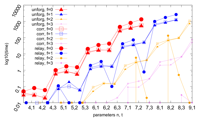
Figure 5: Spin running time on byz.

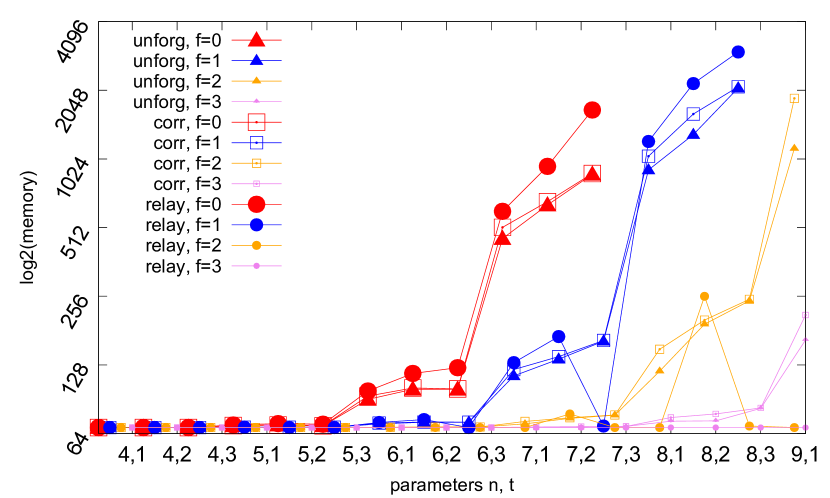
Figure 6: Spin memory usage on byz.

References

- [1] Attiya, H., Welch, J.: Distributed Computing. John Wiley & Sons, 2nd edn. (2004)
- [2] Biely, M., Schmid, U., Weiss, B.: Synchronous consensus under hybrid process and link failures. Theoretical Computer Science 412(40), 5602–5630 (2011)
- [3] Browne, M.C., Clarke, E.M., Grumberg, O.: Reasoning about networks with many identical finite state processes. Inf. Comput. 81, 13–31 (April 1989)
- [4] Chandra, T.D., Toueg, S.: Unreliable failure detectors for reliable distributed systems. J. ACM 43(2), 225–267 (1996)
- [5] Charron-Bost, B., Schiper, A.: The heard-of model: computing in distributed systems with benign faults. Distributed Computing 22(1), 49–71 (2009)
- [6] Clarke, E., Grumberg, O., Peled, D.: Model Checking. MIT Press (1999)
- [7] Clarke, E., Talupur, M., Veith, H.: Proving Ptolemy right: the environment abstraction framework for model checking concurrent systems. In: TACAS’08/ETAPS’08. pp. 33–47. Springer (2008)
- [8] Clarke, E., Talupur, M., Touili, T., Veith, H.: Verification by network decomposition. In: CONCUR 2004. vol. 3170, pp. 276–291 (2004)
- [9] Dolev, D., Dwork, C., Stockmeyer, L.: On the minimal synchronism needed for distributed consensus. J. ACM 34, 77–97 (January 1987)
- [10] Dwork, C., Lynch, N., Stockmeyer, L.: Consensus in the presence of partial synchrony. J. ACM 35(2), 288–323 (Apr 1988)
- [11] Emerson, E., Namjoshi, K.: Reasoning about rings. In: POPL. pp. 85–94 (1995)
- [12] Fischer, M.J., Lynch, N.A., Paterson, M.S.: Impossibility of distributed consensus with one faulty process. J. ACM 32(2), 374–382 (Apr 1985)
- [13] Fisman, D., Kupferman, O., Lustig, Y.: On verifying fault tolerance of distributed protocols. In: TACAS. LNCS, vol. 4963, pp. 315–331. Springer (2008)
- [14] Függer, M., Schmid, U.: Reconciling fault-tolerant distributed computing and systems-on-chip. Distributed Computing 24(6), 323–355 (2012)
- [15] Fuzzati, R., Merro, M., Nestmann, U.: Distributed consensus, revisited. Acta Inf. 44(6), 377–425 (2007)
- [16] Hadzilacos, V., Toueg, S.: Fault-tolerant broadcasts and related problems. In: Mullender, S. (ed.) Distributed Systems, chap. 5, pp. 97–145. Addison-Wesley, 2nd edn. (1993)
- [17] Holzmann, G.: The SPIN Model Checker: Primer and Reference Manual. Addison-Wesley Professional (2003)
- [18] John, A., Konnov, I., Schmid, U., Veith, H., Widder, J.: Counter attack on Byzantine generals: Parameterized model checking of fault-tolerant distributed algorithms. CoRR submit/0572051 (2012)
- [19] Kaynar, D.K., Lynch, N.A., Segala, R., Vaandrager, F.W.: The Theory of Timed I/O Automata. Synthesis Lectures on Computer Science, Morgan&Claypool (2006)
- [20] Lamport, L.: A new solution of dijkstra’s concurrent programming problem. Commun. ACM 17(8), 453–455 (1974)
- [21] Lamport, L.: On interprocess communication. part i: Basic formalism. Distributed Computing 1(2), 77–85 (1986)
- [22] Lamport, L.: Specifying Systems, The TLA+ Language and Tools for Hardware and Software Engineers. Addison-Wesley (2002)
- [23] Lynch, N.: Distributed Algorithms. Morgan Kaufman, San Francisco, USA (1996)
- [24] Lynch, N., Tuttle, M.: An introduction to input/output automata. Tech. Rep. MIT/LCS/TM-373, Laboratory for Computer Science, MIT (1989)
- [25] Mitra, S., Lynch, N.A.: Proving approximate implementations for probabilistic I/O automata. Electr. Notes Theor. Comput. Sci. 174(8), 71–93 (2007)
- [26] Neiger, G., Toueg, S.: Automatically increasing the fault-tolerance of distributed algorithms. J. of Algorithms 11, 374–419 (1990)
- [27] Pease, M., Shostak, R., Lamport, L.: Reaching agreement in the presence of faults. J.ACM 27(2), 228–234 (April 1980)
- [28] Pnueli, A.: The temporal logic of programs. In: FOCS. pp. 46–57 (1977)
- [29] Powell, D.: Failure mode assumptions and assumption coverage. In: FTCS-22. pp. 386–395. Boston, MA, USA (1992)
- [30] Santoro, N., Widmayer, P.: Time is not a healer. In: STACS. LNCS, vol. 349, pp. 304–313. Springer (1989)
- [31] Srikanth, T.K., Toueg, S.: Optimal clock synchronization. Journal of the ACM 34(3), 626–645 (Jul 1987)
- [32] Srikanth, T., Toueg, S.: Simulating authenticated broadcasts to derive simple fault-tolerant algorithms. Distributed Computing 2, 80–94 (1987)
- [33] Widder, J., Schmid, U.: Booting clock synchronization in partially synchronous systems with hybrid process and link failures. Distributed Computing 20(2), 115–140 (August 2007)